Transition Probabilities in Generalized Quantum Search Hamiltonian Evolutions

Abstract

A relevant problem in quantum computing concerns how fast a source state can be driven into a target state according to Schrödinger’s quantum mechanical evolution specified by a suitable driving Hamiltonian. In this paper, we study in detail the computational aspects necessary to calculate the transition probability from a source state to a target state in a continuous time quantum search problem defined by a multi-parameter generalized time-independent Hamiltonian. In particular, quantifying the performance of a quantum search in terms of speed (minimum search time) and fidelity (maximum success probability), we consider a variety of special cases that emerge from the generalized Hamiltonian. In the context of optimal quantum search, we find it is possible to outperform, in terms of minimum search time, the well-known Farhi-Gutmann analog quantum search algorithm. In the context of nearly optimal quantum search, instead, we show it is possible to identify sub-optimal search algorithms capable of outperforming optimal search algorithms if only a sufficiently high success probability is sought. Finally, we briefly discuss the relevance of a tradeoff between speed and fidelity with emphasis on issues of both theoretical and practical importance to quantum information processing.

I Introduction

Grover proposed a quantum algorithm for solving large database search problems in Ref. grover97 ; grover01 . Grover’s search algorithm helps searching for an unknown marked item in an unstructured database of $N$ items by accessing the database a minimum number of times. From a classical standpoint, it is necessary to test $N/2$ items, on average, before finding the correct item. With Grover’s algorithm however, the same task can be completed successfully with a complexity of order $\sqrt{N}$, that is, with a quadratic speed up. Grover’s algorithm was presented in terms of a discrete sequence of unitary logic gates (digital quantum computation). Specifically, the transition probability from the source state $\left|\psi_{s}\right\rangle$ to the target state $\left|\psi_{w}\right\rangle$ after the $k$-times sequential application of the so-called Grover quantum search iterate $G$ is given by,

$$\mathcal{P}_{\text{Grover}}\left(k\text{, }N\right)\overset{\text{def}}{=}\left|\left\langle\psi_{w}|G^{k}|\psi_{s}\right\rangle\right|^{2}=\sin^{2}\left[\left(2k+1\right)\tan^{-1}\left(\frac{1}{\sqrt{N-1}}\right)\right]\text{.}$$ (1)

In the limit of $N$ approaching infinity, $\mathcal{P}_{\text{Grover}}$ in Eq. (1) approaches one if $k=O\left(\sqrt{N}\right)$. We point out that the big $O$-notation $f\left(x\right)=O\left(g\left(x\right)\right)$ means that there exist real constants $c$ and $x_{0}$ such that $\left|f\left(x\right)\right|\leq c\left|g\left(x\right)\right|$ for any $x\geq x_{0}$.

The temporal evolution of the state vector $\left|\psi\left(t\right)\right\rangle$ of a closed quantum system is characterized by the Schrödinger equation,

$$i\hslash\partial_{t}\left|\psi\left(t\right)\right\rangle=\mathcal{H}\left(t\right)\left|\psi\left(t\right)\right\rangle\text{,}$$ (2)

where $\hslash\overset{\text{def}}{=}h/\left(2\pi\right)$ is the reduced Planck constant, $i$ denotes the imaginary complex unit, and $\partial_{t}\overset{\text{def}}{=}\partial/\partial t$. The Hamiltonian $\mathcal{H}\left(t\right)$ in Eq. (2) encodes all relevant information about the time evolution of the quantum system. From a quantum computing standpoint, if the Hamiltonian $\mathcal{H}\left(t\right)$ is known and properly designed, the quantum mechanical motion is known and the initial state (source state, $\left|\psi_{s}\right\rangle$) at $t=0$ can potentially evolve to a given final state (target state, $\left|\psi_{w}\right\rangle$) at $t=T$. In particular, for any instant $0\leq t\leq T$, the probability $\mathcal{P}_{\left|\psi\left(t\right)\right\rangle\rightarrow\left|\psi_{w}\right\rangle}$ that the system transitions from the state $\left|\psi\left(t\right)\right\rangle$ to the state $\left|\psi_{w}\right\rangle$ under the working assumption of constant Hamiltonian is given by,

$$\mathcal{P}_{\left|\psi\left(t\right)\right\rangle\rightarrow\left|\psi_{w}\right\rangle}\overset{\text{def}}{=}\left|\left\langle\psi_{w}|\psi\left(t\right)\right\rangle\right|^{2}=\left|\left\langle\psi_{w}|e^{-\frac{i}{\hslash}\mathcal{H}t}|\psi_{s}\right\rangle\right|^{2}\text{.}$$ (3)

The unitary operator $\mathcal{U}\left(t\right)\overset{\text{def}}{=}e^{-\frac{i}{\hslash}\mathcal{H}t}$ denotes the temporal evolution operator. Fig. $1$ displays a graphical depiction of the digital (discrete time) and analog (continuous time) quantum search algorithms.

Working in a continuous time quantum computing framework, Farhi and Gutmann proposed an analog version of Grover’s algorithm in Ref. farhi98 where the state of the quantum register evolves continuously in time under the action of a suitably chosen driving Hamiltonian (analog quantum computation). Specifically, the transition probability from the source state $\left|\psi_{s}\right\rangle$ to the target state $\left|\psi_{w}\right\rangle$ after the application of the unitary continuous time evolution operator $\mathcal{U}_{\text{FG}}\left(t\right)\overset{\text{def}}{=}e^{-\frac{i}{\hslash}\mathcal{H}_{\text{FG}}t}$ for a closed quantum system described by a constant Hamiltonian $\mathcal{H}_{\text{FG}}$ is given by,

$$\mathcal{P}_{\text{Farhi-Gutmann}}\left(t\text{, }x\right)\overset{\text{def}}{=}\left|\left\langle\psi_{w}|e^{-\frac{i}{\hslash}\mathcal{H}_{\text{FG}}t}|\psi_{s}\right\rangle\right|^{2}=\sin^{2}\left(\frac{Ex}{\hslash}t\right)+x^{2}\cos^{2}\left(\frac{Ex}{\hslash}t\right)\text{,}$$ (4)

where $E$ is a energy-like positive and real constant coefficient. We point out that $\mathcal{P}_{\text{Farhi-Gutmann}}$ in Eq. (4) approaches one if $t$ approaches $h/(4Ex)$. For recent discussions on the transition from the digital to analog quantum computational setting for Grover’s algorithm, we refer to Ref. carlo1 ; carlo2 ; cafaro2017 .

Ideally, one seeks to achieve unit success probability (that is, unit fidelity) in the shortest possible time in a quantum search problem. There are however, both practical and foundational issues that can justify the exploration of alternative circumstances. For instance, from a practical standpoint, one would desire to terminate a quantum information processing task in the minimum possible time so as to mitigate decoherent effects that can appear while controlling (by means of an external magnetic field, for instance) the dynamics of a source state driven towards a target state rabitz12 ; rabitz15 ; cappellaro18 . In addition, from a theoretical viewpoint, it is known that no quantum measurement can perfectly discriminate between two nonorthogonal pure states chefles00 ; croke09 . Moreover, it is equally notorious that suitably engineered quantum measurements can enhance the transition probability between two pure states fritz10 . Therefore, minimizing the search time can be important from an experimental standpoint while seeking at any cost perfect overlap between the final state and the target state can be unnecessary from a purely foundational standpoint. Similar lines of reasoning have paved the way to the fascinating exploration of a possible tradeoff between fidelity and time optimal control of quantum unitary transformations in Ref. rabitz12 .

In this paper, motivated by these issues and starting from the consideration of a family of multi-parameter generalized quantum search Hamiltonians originally introduced by Bae and Kwon in Ref. bae02 , we present a detailed analysis concerning minimum search times and maximal success probabilities that can be obtained from suitably chosen sub-families belonging to the original family of Hamiltonians. In particular, we uncover the existence of quantum search Hamiltonians characterized by minimum search times needed for a perfect search that are smaller than the one required by the Farhi-Gutmann perfect quantum search Hamiltonian. Furthermore, and more interestingly, we report on the existence of imperfect quantum search Hamiltonians that, despite being incapable of guaranteeing perfect search, can outperform (in terms of minimum search time) perfect search Hamiltonians provided that only a very large nearly optimal fidelity value is required to stop the search.

The layout of the rest of the paper can be described as follows. In Section II, we provide a detailed computation of a general expression for the transition probability in the case of a quantum mechanical evolution governed by a time-independent generalized quantum search Hamiltonian. In Section III, we discuss a variety of limiting cases that arise from the generalized search Hamiltonian. In particular, we distinguish optimal scenarios (that is, cases where the probability of finding the target state equals one) from suboptimal scenarios (that is, cases where the probability of finding the target state is less than one). Our concluding remarks appear in Section IV. Finally, technical details are presented in Appendices A, B, and C.

Figure 1: Gate-level schematic of the (a) digital and (b) analog quantum search algorithms.

II Transition probability

In this section, we consider the time-independent search Hamiltonian $\mathcal{H}$ defined as bae02 ,

$$\mathcal{H}\overset{\text{def}}{=}E\left[\alpha\left|\psi_{w}\right\rangle\left\langle\psi_{w}\right|+\beta\left|\psi_{w}\right\rangle\left\langle\psi_{s}\right|+\gamma\left|\psi_{s}\right\rangle\left\langle\psi_{w}\right|+\delta\left|\psi_{s}\right\rangle\left\langle\psi_{s}\right|\right]\text{.}$$ (5)

The adimensional coefficients $\alpha$, $\beta$, $\gamma$, $\delta$ in Eq. (5) are complex expansion coefficients while $E$ is a real constant with energy physical dimensions. We also assume that the quantum state $\left|\psi_{w}\right\rangle$ is the normalized target state while $\left|\psi_{s}\right\rangle$ is the normalized initial state with quantum overlap $x\overset{\text{def}}{=}\left\langle\psi_{w}|\psi_{s}\right\rangle$ that evolves unitarily according to the Schrödinger quantum mechanical evolution law,

$$\left|\psi_{s}\right\rangle\mapsto e^{-\frac{i}{\hslash}\mathcal{H}t}\left|\psi_{s}\right\rangle\text{.}$$ (6)

In general, $x$ is a complex quantity. However, since any phase factor $e^{i\phi_{ws}}$ with $\phi_{ws}\in\mathbb{R}$ in $x\overset{\text{def}}{=}\left\langle\psi_{w}|\psi_{s}\right\rangle=\left|\left\langle\psi_{w}|\psi_{s}\right\rangle\right|e^{i\phi_{ws}}$ can be incorporated into the state $\left|s\right\rangle$, one can assume that $x\in\mathbb{R}_{+}\backslash\left\{0\right\}$. Our objective is to find the time $t^{\ast}$ such that $\mathcal{P}\left(t^{\ast}\right)=\mathcal{P}_{\max}$ where $\mathcal{P}\left(t\right)$ is the transition probability defined as sakurai ; picasso ,

$$\mathcal{P}\left(t\right)\overset{\text{def}}{=}\left|\left\langle\psi_{w}|e^{-\frac{i}{\hslash}\mathcal{H}t}|\psi_{s}\right\rangle\right|^{2}\text{.}$$ (7)

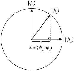
Figure 2: Visualization of the normalized states $\left|\psi_{w}\right\rangle$, $\left|\psi_{s}\right\rangle$, and $\left|\psi_{r}\right\rangle$, as well as the quantum overlap $x$.

Using the Gram-Schmidt orthonormalization technique, we can construct an orthonormal set of quantum state vectors starting from the set $\left\{\left|\psi_{w}\right\rangle\text{, }\left|\psi_{s}\right\rangle\right\}$. The transition from a set of linear independent state vectors to a set of orthonormal state vector can be described as,

$$\left\{\left|\psi_{w}\right\rangle\text{, }\left|\psi_{s}\right\rangle\right\}\rightarrow\left\{\left|\psi_{w}\right\rangle\text{, }\left|\psi_{s}\right\rangle-\left\langle\psi_{s}|\psi_{w}\right\rangle\left|\psi_{w}\right\rangle\right\}\rightarrow\left\{\frac{\left|\psi_{w}\right\rangle}{\left\|\left|\psi_{w}\right\rangle\right\|}\text{, }\frac{\left|\psi_{s}\right\rangle-\left\langle\psi_{s}|\psi_{w}\right\rangle\left|\psi_{w}\right\rangle}{\left\|\left|\psi_{s}\right\rangle-\left\langle\psi_{s}|\psi_{w}\right\rangle\left|\psi_{w}\right\rangle\right\|}\right\}\text{.}$$ (8)

For notational simplicity, let us define the quantum state vector $\left|\psi_{r}\right\rangle$ as

$$\left|\psi_{r}\right\rangle\overset{\text{def}}{=}\frac{\left|\psi_{s}\right\rangle-\left\langle\psi_{s}|\psi_{w}\right\rangle\left|\psi_{w}\right\rangle}{\left\|\left|\psi_{s}\right\rangle-\left\langle\psi_{s}|\psi_{w}\right\rangle\left|\psi_{w}\right\rangle\right\|}\text{.}$$ (9)

Recalling the definition of the quantum overlap $x$, Eq. (9) can be expressed as,

$$\left|\psi_{r}\right\rangle=\frac{\left|\psi_{s}\right\rangle-\left\langle\psi_{s}|\psi_{w}\right\rangle\left|\psi_{w}\right\rangle}{\sqrt{\left\langle\psi_{s}|\psi_{s}\right\rangle-\left\langle\psi_{s}|\psi_{w}\right\rangle^{2}}}=\frac{1}{\sqrt{1-x^{2}}}\left(\left|\psi_{s}\right\rangle-x\left|\psi_{w}\right\rangle\right)\text{.}$$ (10)

Fig. $2$ displays a graphical depiction of the orthonormal states $\left\{\left|\psi_{w}\right\rangle\text{, }\left|\psi_{r}\right\rangle\right\}$ together with the source state $\left|\psi_{s}\right\rangle$ and the quantum overlap $x$. Fig. $3$, instead, is a simple depiction of the orthogonalization and normalization procedures that specify the Gram-Schmidt orthonormalization technique. Note that because of the definition of $\left|\psi_{r}\right\rangle$ in Eq. (10), $x$ must be different from one. In terms of the set of orthonormal basis vectors $\left\{\left|\psi_{w}\right\rangle\text{, }\left|\psi_{r}\right\rangle\right\}$, the source state $\left|\psi_{s}\right\rangle$ becomes

$$\left|\psi_{s}\right\rangle=\left|\psi_{s}\right\rangle\left(\left|\psi_{w}\right\rangle\left\langle\psi_{w}\right|+\left|\psi_{r}\right\rangle\left\langle\psi_{r}\right|\right)=\left\langle\psi_{w}|\psi_{s}\right\rangle\left|\psi_{w}\right\rangle+\left\langle\psi_{r}|\psi_{s}\right\rangle\left|\psi_{r}\right\rangle\text{.}$$ (11)

Note that the quantum mechanical overlap $\left\langle\psi_{r}|\psi_{s}\right\rangle$ in Eq. (11) can be recast as,

$$\left\langle\psi_{r}|\psi_{s}\right\rangle=\frac{1}{\sqrt{1-x^{2}}}\left(\left\langle\psi_{s}\right|-x\left\langle\psi_{w}\right|\right)\left(\left|\psi_{s}\right\rangle\right)=\frac{1}{\sqrt{1-x^{2}}}\left(1-x^{2}\right)=\sqrt{1-x^{2}}\text{.}$$ (12)

Therefore, by using Eq. (12), the state $\left|\psi_{s}\right\rangle$ in Eq. (11) becomes

$$\left|\psi_{s}\right\rangle=x\left|\psi_{w}\right\rangle+\sqrt{1-x^{2}}\left|\psi_{r}\right\rangle\text{.}$$ (13)

The matrix representation of the Hamiltonian $\mathcal{H}$ in Eq. (5) with respect to the orthonormal basis $\left\{\left|\psi_{w}\right\rangle\text{, }\left|\psi_{r}\right\rangle\right\}$ where $\left\langle\psi_{w}|\psi_{r}\right\rangle=\delta_{wr}$, with $\delta_{wr}$ denoting the Kronecker delta, can be formally written as

$$\left[\mathcal{H}\right]_{\left\{\left|\psi_{w}\right\rangle\text{, }\left|\psi_{r}\right\rangle\right\}}\overset{\text{def}}{=}\left(\begin{array}[c]{cc}\left\langle\psi_{w}|\mathcal{H}|\psi_{w}\right\rangle&\left\langle\psi_{w}|\mathcal{H}|\psi_{r}\right\rangle\\ \left\langle\psi_{r}|\mathcal{H}|\psi_{w}\right\rangle&\left\langle\psi_{r}|\mathcal{H}|\psi_{r}\right\rangle\end{array}\right)\text{.}$$ (14)

Using Eqs. (5) and (13) together with the orthonormality conditions $\left\langle\psi_{w}|\psi_{r}\right\rangle=\delta_{wr}$, we have

$$\left[\mathcal{H}\right]_{\left\{\left|\psi_{w}\right\rangle\text{, }\left|\psi_{r}\right\rangle\right\}}=\left(\begin{array}[c]{cc}H_{11}&H_{12}\\ H_{21}&H_{22}\end{array}\right)\text{,}$$ (15)

where,

$$H_{11}\overset{\text{def}}{=}E\left[\alpha+\left(\beta+\gamma\right)x+\delta x^{2}\right]\text{, }H_{12}\overset{\text{def}}{=}E\sqrt{1-x^{2}}\left(\beta+\delta x\right)\text{,}$$

$$H_{21}\overset{\text{def}}{=}E\sqrt{1-x^{2}}\left(\gamma+\delta x\right)\text{, }H_{22}\overset{\text{def}}{=}E\delta\left(1-x^{2}\right)\text{.}$$ (16)

Figure 3: Illustration of the Gram-Schmidt orthonormalization procedure for some vectors $\left|a\right\rangle$ and $\left|b\right\rangle$. In this case, the resulting orthonormal basis consists of $\left|e_{1}\right\rangle\overset{\text{def}}{=}\frac{\left|a\right\rangle}{\left\|\left|a\right\rangle\right\|}$ and $\left|e_{2}\right\rangle\overset{\text{def}}{=}\frac{\left|b\right\rangle-\left\langle a|b\right\rangle\left|a\right\rangle}{\left\|\left|b\right\rangle-\left\langle a|b\right\rangle\left|a\right\rangle\right\|}$.

Observe that the Hamiltonian $\mathcal{H}$ is an Hermitian operator and, therefore, its eigenvalues must be real (for details, see Appendix A). For this reason, recalling the previous constraints on $x$, we finally have $x\in\left(0\text{,}1\right)$. Furthermore, imposing that $\mathcal{H}=\mathcal{H}^{\dagger}$ where the dagger symbol “$\dagger$” is the Hermitian conjugation operation, we have

$$\left(\begin{array}[c]{cc}H_{11}&H_{12}\\ H_{21}&H_{22}\end{array}\right)=\left(\begin{array}[c]{cc}H_{11}^{\ast}&H_{21}^{\ast}\\ H_{12}^{\ast}&H_{22}^{\ast}\end{array}\right)\text{.}$$ (17)

Then, from Eqs. (16) and (17), it follows that $\alpha$ and $\delta$ must be real coefficients while $\beta=\gamma^{\ast}$. The symbol “$\ast$” denotes the complex conjugation operation. Next, let us diagonalize the Hermitian matrix $\left[\mathcal{H}\right]_{\left\{\left|\psi_{w}\right\rangle\text{, }\left|\psi_{r}\right\rangle\right\}}$ in Eq. (15). The two real eigenvalues $\lambda_{\pm}$ of the matrix can be written as,

$$\lambda_{\pm}\overset{\text{def}}{=}\frac{1}{2}\left[\left(H_{11}+H_{22}\right)\pm\sqrt{\left(H_{11}-H_{22}\right)^{2}+4H_{12}H_{21}}\right]\text{.}$$ (18)

The eigenspaces $\mathcal{E}_{\lambda_{-}}$ and $\mathcal{E}_{\lambda_{+}}$ that correspond to the eigenvalues $\lambda_{-}$ and $\lambda_{+}$ are defined as

$$\mathcal{E}_{\lambda_{-}}\overset{\text{def}}{=}\text{{Span}}\left\{\left|v_{\lambda_{-}}\right\rangle\right\}\text{, and }\mathcal{E}_{\lambda_{+}}\overset{\text{def}}{=}\text{{Span}}\left\{\left|v_{\lambda_{+}}\right\rangle\right\}\text{,}$$ (19)

respectively. Furthermore, two orthogonal eigenvectors $\left|v_{\lambda_{+}}\right\rangle$ and $\left|v_{\lambda_{-}}\right\rangle$ corresponding to the distinct eigenvalues $\lambda_{+}$ and $\lambda_{-}$ are given by,

$$\left|v_{\lambda_{+}}\right\rangle\overset{\text{def}}{=}\left(\begin{array}[c]{c}\frac{1}{2H_{21}}\left[\left(H_{11}-H_{22}\right)+\sqrt{\left(H_{11}-H_{22}\right)^{2}+4H_{12}H_{21}}\right]\\ 1\end{array}\right)\text{,}$$ (20)

and,

$$\left|v_{\lambda_{-}}\right\rangle\overset{\text{def}}{=}\left(\begin{array}[c]{c}\frac{1}{2H_{21}}\left[\left(H_{11}-H_{22}\right)-\sqrt{\left(H_{11}-H_{22}\right)^{2}+4H_{12}H_{21}}\right]\\ 1\end{array}\right)\text{,}$$ (21)

respectively. For notational simplicity, let us introduce two complex quantities $\mathcal{A}$ and $\mathcal{B}$ defined as

$$\mathcal{A}\overset{\text{def}}{=}\frac{1}{2H_{21}}\left[\left(H_{11}-H_{22}\right)-\sqrt{\left(H_{11}-H_{22}\right)^{2}+4H_{12}H_{21}}\right]\text{,}$$ (22)

and,

$$\mathcal{B}\overset{\text{def}}{=}\frac{1}{2H_{21}}\left[\left(H_{11}-H_{22}\right)+\sqrt{\left(H_{11}-H_{22}\right)^{2}+4H_{12}H_{21}}\right]\text{,}$$ (23)

respectively. Using Eqs. (20), (21), (22), and (23), the eigenvector matrix $M_{\mathcal{H}}$ for the matrix $\left[\mathcal{H}\right]_{\left\{\left|\psi_{w}\right\rangle\text{, }\left|\psi_{r}\right\rangle\right\}}$ and its inverse $M_{\mathcal{H}}^{-1}$ can be formally written as,

$$M_{\mathcal{H}}\overset{\text{def}}{=}\left(\begin{array}[c]{cc}\mathcal{A}&\mathcal{B}\\ 1&1\end{array}\right)\text{,}$$ (24)

and,

$$M_{\mathcal{H}}^{-1}\overset{\text{def}}{=}\frac{1}{\mathcal{A}-\mathcal{B}}\left(\begin{array}[c]{cc}1&-\mathcal{B}\\ -1&\mathcal{A}\end{array}\right)=M_{\mathcal{H}}^{\dagger}\text{,}$$ (25)

respectively. In terms of the matrices $M_{\mathcal{H}}$ in Eq. (24), $M_{\mathcal{H}}^{-1}$ in Eq. (25), and the diagonal matrix $H_{\text{diagonal}}$ defined as,

$$H_{\text{diagonal}}\overset{\text{def}}{=}\left[\mathcal{H}\right]_{\left\{\left|v_{\lambda-}\right\rangle\text{, }\left|v_{\lambda_{+}}\right\rangle\right\}}=\left(\begin{array}[c]{cc}\left\langle v_{\lambda-}|\mathcal{H}|v_{\lambda-}\right\rangle&\left\langle v_{\lambda-}|\mathcal{H}|v_{\lambda_{+}}\right\rangle\\ \left\langle v_{\lambda_{+}}|\mathcal{H}|v_{\lambda-}\right\rangle&\left\langle v_{\lambda_{+}}|\mathcal{H}|v_{\lambda_{+}}\right\rangle\end{array}\right)=\left(\begin{array}[c]{cc}\lambda_{-}&0\\ 0&\lambda_{+}\end{array}\right)\text{,}$$ (26)

the matrix $\left[\mathcal{H}\right]_{\left\{\left|\psi_{w}\right\rangle\text{, }\left|\psi_{r}\right\rangle\right\}}$ in Eq. (15) becomes

$$\left[\mathcal{H}\right]_{\left\{\left|\psi_{w}\right\rangle\text{, }\left|\psi_{r}\right\rangle\right\}}=M_{\mathcal{H}}H_{\text{diagonal}}M_{\mathcal{H}}^{-1}=\left(\begin{array}[c]{cc}\mathcal{A}&\mathcal{B}\\ 1&1\end{array}\right)\left(\begin{array}[c]{cc}\lambda_{-}&0\\ 0&\lambda_{+}\end{array}\right)\left(\begin{array}[c]{cc}\frac{1}{\mathcal{A}-\mathcal{B}}&\frac{-\mathcal{B}}{\mathcal{A}-\mathcal{B}}\\ \frac{-1}{\mathcal{A}-\mathcal{B}}&\frac{\mathcal{A}}{\mathcal{A}-\mathcal{B}}\end{array}\right)\text{.}$$ (27)

We recall that the eigenvalues in Eq. (26) are defined in Eq. (18) while $\mathcal{A}$ and $\mathcal{B}$ appear in Eqs. (22) and (23), respectively. At this juncture, we also recall that our objective is to find the time $t^{\ast}$ such that $\mathcal{P}\left(t^{\ast}\right)=\mathcal{P}_{\max}$ where the transition probability $\mathcal{P}\left(t\right)$ is defined in Eq. (7). Employing standard linear algebra techniques, $\mathcal{P}\left(t\right)$ can be recast as

$$\mathcal{P}\left(t\right)\overset{\text{def}}{=}\left|\left\langle\psi_{w}|e^{-\frac{i}{\hslash}\mathcal{H}t}|\psi_{s}\right\rangle\right|^{2}=\left|\left\langle\psi_{w}|e^{-\frac{i}{\hslash}M\mathcal{H}_{\text{diagonal}}M^{\dagger}t}|\psi_{s}\right\rangle\right|^{2}=\left|\left\langle\psi_{w}|Me^{-\frac{i}{\hslash}\mathcal{H}_{\text{diagonal}}t}M^{\dagger}|\psi_{s}\right\rangle\right|^{2}\text{,}$$ (28)

where $\mathcal{H}_{\text{diagonal}}$ denotes the Hermitian operator whose matrix representation is $H_{\text{diagonal}}$ in Eq. (26). Using the matrix notation with components expressed with respect to the orthonormal basis $\left\{\left|\psi_{w}\right\rangle\text{, }\left|\psi_{r}\right\rangle\right\}$, quantum states $\left|\psi_{w}\right\rangle$ and $\left|\psi_{s}\right\rangle$ are given by

$$\left|\psi_{w}\right\rangle\overset{\text{def}}{=}\left(\begin{array}[c]{c}1\\ 0\end{array}\right)\text{, and }\left|\psi_{s}\right\rangle\overset{\text{def}}{=}\left(\begin{array}[c]{c}x\\ \sqrt{1-x^{2}}\end{array}\right)\text{,}$$ (29)

respectively. By means of Eqs. (24), (25), and (29), the quantum state amplitude $\left\langle\psi_{w}|e^{-\frac{i}{\hslash}\mathcal{H}t}|\psi_{s}\right\rangle$ that appears in the expression of the fidelity $\mathcal{P}\left(t\right)$ in Eq. (28) becomes

$$\left\langle\psi_{w}|e^{-\frac{i}{\hslash}\mathcal{H}t}|\psi_{s}\right\rangle=\frac{1}{\mathcal{A}-\mathcal{B}}\left[\mathcal{A}e^{-\frac{i}{\hslash}\lambda_{-}t}\left(x-\mathcal{B}\sqrt{1-x^{2}}\right)-\mathcal{B}e^{-\frac{i}{\hslash}\lambda_{+}t}\left(x-\mathcal{A}\sqrt{1-x^{2}}\right)\right]\text{,}$$ (30)

and, as a consequence, its complex conjugate $\left\langle\psi_{w}|e^{-\frac{i}{\hslash}\mathcal{H}t}|\psi_{s}\right\rangle^{\ast}$ is,

$$\left\langle\psi_{w}|e^{-\frac{i}{\hslash}\mathcal{H}t}|\psi_{s}\right\rangle^{\ast}=\frac{1}{\mathcal{A}-\mathcal{B}}\left[\mathcal{A}e^{\frac{i}{\hslash}\lambda_{-}t}\left(x-\mathcal{B}\sqrt{1-x^{2}}\right)-\mathcal{B}e^{\frac{i}{\hslash}\lambda_{+}t}\left(x-\mathcal{A}\sqrt{1-x^{2}}\right)\right]\text{.}$$ (31)

Observe that,

$$e^{-\frac{i}{\hslash}\lambda_{-}t}=e^{-\frac{i}{\hslash}\frac{H_{11}+H_{22}}{2}t}e^{i\frac{\mathrm{a}}{\hslash}t}\text{ and, }e^{-\frac{i}{\hslash}\lambda_{+}t}=e^{-\frac{i}{\hslash}\frac{H_{11}+H_{22}}{2}t}e^{-i\frac{\mathrm{a}}{\hslash}t}$$ (32)

where, recalling Eq. (18), the real quantity $\mathrm{a}$ is defined as

$$\mathrm{a}\overset{\text{def}}{=}\frac{1}{2}\sqrt{\left(H_{11}-H_{22}\right)^{2}+4H_{12}H_{21}}\text{.}$$ (33)

Employing Eq. (32), the complex probability amplitudes in Eqs. (30) and (31) become

$$\left\langle\psi_{w}|e^{-\frac{i}{\hslash}\mathcal{H}t}|\psi_{s}\right\rangle=e^{-\frac{i}{\hslash}\frac{H_{11}+H_{22}}{2}t}\left[\frac{\mathcal{A}\left(x-\mathcal{B}\sqrt{1-x^{2}}\right)}{\mathcal{A}-\mathcal{B}}e^{i\frac{\mathrm{a}}{\hslash}t}-\frac{\mathcal{B}\left(x-\mathcal{A}\sqrt{1-x^{2}}\right)}{\mathcal{A}-\mathcal{B}}e^{-i\frac{\mathrm{a}}{\hslash}t}\right]\text{,}$$ (34)

and,

$$\left\langle\psi_{w}|e^{-\frac{i}{\hslash}\mathcal{H}t}|\psi_{s}\right\rangle^{\ast}=e^{\frac{i}{\hslash}\frac{H_{11}+H_{22}}{2}t}\left[\frac{\mathcal{A}^{\ast}\left(x-\mathcal{B}^{\ast}\sqrt{1-x^{2}}\right)}{\mathcal{A}^{\ast}-\mathcal{B}^{\ast}}e^{-i\frac{\mathrm{a}}{\hslash}t}-\frac{\mathcal{B}^{\ast}\left(x-\mathcal{A}^{\ast}\sqrt{1-x^{2}}\right)}{\mathcal{A}^{\ast}-\mathcal{B}^{\ast}}e^{i\frac{\mathrm{a}}{\hslash}t}\right]\text{,}$$ (35)

respectively. Using Eqs. (34) and (35) and introducing the following three quantities

$$\tilde{A}\overset{\text{def}}{=}\frac{\mathcal{A}\left(x-\mathcal{B}\sqrt{1-x^{2}}\right)}{\mathcal{A}-\mathcal{B}}\text{, }\tilde{B}\overset{\text{def}}{=}-\frac{\mathcal{B}\left(x-\mathcal{A}\sqrt{1-x^{2}}\right)}{\mathcal{A}-\mathcal{B}}\text{, and }\tilde{\alpha}=\frac{\mathrm{a}}{\hslash}t\text{,}$$ (36)

the transition probability $\mathcal{P}\left(t\right)$ in Eq. (7) can be written as

$$\mathcal{P}\left(\tilde{\alpha}\right)=\left[\tilde{A}e^{i\tilde{\alpha}}+\tilde{B}e^{-i\tilde{\alpha}}\right]\left[\tilde{A}^{\ast}e^{-i\tilde{\alpha}}+\tilde{B}^{\ast}e^{i\tilde{\alpha}}\right]=\left|\tilde{A}\right|^{2}+\left|\tilde{B}\right|^{2}+2\tilde{A}\tilde{B}^{\ast}\cos\left(2\tilde{\alpha}\right)\text{,}$$ (37)

where we point out that $\tilde{A}\tilde{B}^{\ast}$ is real since $H_{12}=H_{21}^{\ast}$. By employing standard trigonometric identities in a convenient sequential order (for details, see Appendix B), we find

$$\mathcal{P}\left(\tilde{\alpha}\right)=\left|\tilde{A}-\tilde{B}\right|^{2}\sin^{2}\left(\tilde{\alpha}\right)+\left|\tilde{A}+\tilde{B}\right|^{2}\cos^{2}\left(\tilde{\alpha}\right)\text{.}$$ (38)

Using Eqs. (36), (33), (22), and (23), the transition probability $\mathcal{P}\left(\tilde{\alpha}\right)$ in Eq. (38) becomes

$$\mathcal{P}\left(t\right)=\frac{\left|\left(H_{11}-H_{22}\right)x+2H_{12}\sqrt{1-x^{2}}\right|^{2}}{\left(H_{11}-H_{22}\right)^{2}+4H_{12}H_{21}}\sin^{2}\left(\frac{\sqrt{\left(H_{11}-H_{22}\right)^{2}+4H_{12}H_{21}}}{2\hslash}t\right)+x^{2}\cos^{2}\left(\frac{\sqrt{\left(H_{11}-H_{22}\right)^{2}+4H_{12}H_{21}}}{2\hslash}t\right)\text{.}$$ (39)

From Eq. (39), it follows that the maximum $\mathcal{P}_{\max}=\mathcal{P}\left(t^{\ast}\right)$ of $\mathcal{P}\left(t\right)$ occurs at the instant $t^{\ast}$,

$$t^{\ast}\overset{\text{def}}{=}\frac{\pi\hslash}{\sqrt{\left(H_{11}-H_{22}\right)^{2}+4H_{12}H_{21}}}\text{,}$$ (40)

and equals

$$\mathcal{P}_{\max}=\frac{\left|\left(H_{11}-H_{22}\right)x+2H_{12}\sqrt{1-x^{2}}\right|^{2}}{\left(H_{11}-H_{22}\right)^{2}+4H_{12}H_{21}}\text{.}$$ (41)

Finally, making use of Eq.(16) and recalling that $\alpha$ and $\delta$ must be real coefficients while $\beta=\gamma^{\ast}$, $\mathcal{P}_{\max}$ in Eq. (41) becomes

$$\mathcal{P}_{\max}\left(\alpha\text{, }\beta\text{, }\delta\text{, }x\right)=\frac{\left|\left[\left(\alpha-\delta\right)+\left(\beta+\beta^{\ast}\right)x+2\delta x^{2}\right]x+2\left(\beta+\delta x\right)\left(1-x^{2}\right)\right|^{2}}{\left[\left(\alpha-\delta\right)+\left(\beta+\beta^{\ast}\right)x+2\delta x^{2}\right]^{2}+4\left(1-x^{2}\right)\left(\beta+\delta x\right)\left(\beta^{\ast}+\delta x\right)}\text{.}$$ (42)

Note that $\gamma=\beta^{\ast}$, $\beta+\beta^{\ast}=2\operatorname{Re}\left(\beta\right)\in\mathbb{R}$, and the product $\left(\beta+\delta x\right)\left(\beta^{\ast}+\delta x\right)$ is a real quantity for any complex parameter $\beta$.

III Discussion

In this section, we discuss a variety of limiting cases that arise from the generalized search Hamiltonian in Eq. (5). In particular, we make a distinction between optimal and suboptimal scenarios. The former scenarios are cases where the probability of finding the target state equals one. The latter scenarios, instead, are cases where the probability of finding the target state is less than one.

General Case: The general case is specified by the conditions $\alpha\neq\delta$ real and $\beta=\gamma^{\ast}$ complex coefficients. We note that after some straightforward but tedious algebra, $\mathcal{P}_{\max}$ in Eq. (42) can be recast as

$$\mathcal{P}_{\max}\left(\alpha\text{, }\beta\text{, }\delta\text{, }x\right)=\frac{4\left[\left|\beta\right|^{2}-\operatorname{Re}^{2}\left(\beta\right)\right]x^{4}+\left[\left(\alpha+\delta\right)^{2}-8\left(\left|\beta\right|^{2}-\operatorname{Re}^{2}\left(\beta\right)\right)\right]x^{2}+4\operatorname{Re}\left(\beta\right)\left(\alpha+\delta\right)x+4\left|\beta\right|^{2}}{4\left[\alpha\delta+\operatorname{Re}^{2}\left(\beta\right)-\left|\beta\right|^{2}\right]x^{2}+4\operatorname{Re}\left(\beta\right)\left(\alpha+\delta\right)x+\left[\left(\alpha-\delta\right)^{2}+4\left|\beta\right|^{2}\right]}\text{.}$$ (43)

Furthermore, by using Eq. (16) in Eq. (40), the time $t^{\ast}$ at which this maximum transition probability value $\mathcal{P}_{\max}$ is achieved becomes,

$$t_{\mathcal{H}}^{\ast}\overset{\text{def}}{=}\frac{\pi\hslash}{E\sqrt{\left[\left(\alpha-\delta\right)+x\left(\beta+\beta^{\ast}\right)+2x^{2}\delta\right]^{2}+4\left(1-x^{2}\right)\left(\beta+\delta x\right)\left(\beta^{\ast}+\delta x\right)}}\text{.}$$ (44)

The subscript $\mathcal{H}$ in $t_{\mathcal{H}}^{\ast}$ denotes the generalized search Hamiltonian in Eq. (5). Observe that $t_{\mathcal{H}}^{\ast}$ in Eq. (44) can be rewritten as,

$$t_{\mathcal{H}}^{\ast}\overset{\text{def}}{=}\frac{2}{\sqrt{4\left[\alpha\delta+\operatorname{Re}^{2}\left(\beta\right)-\left|\beta\right|^{2}\right]x^{2}+4\operatorname{Re}\left(\beta\right)\left(\alpha+\delta\right)x+\left[\left(\alpha-\delta\right)^{2}+4\left|\beta\right|^{2}\right]}}\frac{\pi\hslash}{2E}\text{.}$$ (45)

Case	$\alpha$	$\beta$	$\gamma$	$\delta$	${\mathcal{P}}_{\text{max}}$
General	$\neq\delta$	$\gamma^{*}\in\mathbb{C}$	$\beta^{*}\in\mathbb{C}$	$\neq\alpha$	$\leq 1$
1	$\delta$	$0$	$0$	$\alpha$	$1$
2	$\neq\delta$	$0$	$0$	$\neq\alpha$	$\leq 1$
3	$0$	$\gamma^{*}\in\mathbb{R}$	$\beta^{*}\in\mathbb{R}$	$0$	$1$
4	$0$	$\gamma*\in\mathbb{C}$	$\beta^{*}\in\mathbb{C}$	$0$	$\leq 1$
5	$\delta$	$\gamma^{*}\in\mathbb{R}$	$\beta^{*}\in\mathbb{R}$	$\alpha$	$1$
6	$\delta$	$\gamma^{*}\in\mathbb{C}$	$\beta^{*}\in\mathbb{C}$	$\alpha$	$\leq 1$
7	$\neq\delta$	$\gamma^{*}\in\mathbb{R}$	$\beta^{*}\in\mathbb{R}$	$\neq\alpha$	$\leq 1$

Table 1: Summary of maximal success probability values $\mathcal{P}_{\max}$ that can be achieved for a variety of choices of the parameters $\alpha$, $\beta$, $\gamma$, and $\delta$ specifying the quantum search Hamiltonian $\mathcal{H}$ in Eq. (5).

In what follows, we choose to briefly discuss a number of limiting cases that arise from Eq. (43). In particular, the big-calligraphic-$\mathcal{O}$ notation $f\left(\varepsilon\right)=\mathcal{O}\left(g\left(\varepsilon\right)\right)$ means that $f\left(\varepsilon\right)$ is an infinitesimal of order equal to $g\left(\varepsilon\right)$ as $\varepsilon$ approaches zero, that is,

$$\lim_{\varepsilon\rightarrow 0}\frac{f\left(\varepsilon\right)}{g\left(\varepsilon\right)}=K\text{,}$$ (46)

where $K$ denotes a nonzero real constant. In Table I we report an overview of the maximal success probability values that can be obtained for a variety of choices of the parameters $\alpha$, $\beta$, $\gamma$, and $\delta$ characterizing the quantum search Hamiltonian $\mathcal{H}$. In particular, we note that the unit success probability $\mathcal{P}_{\max}=1$ can be achieved only when considering the Hamiltonians $\mathcal{H}_{1}$, $\mathcal{H}_{3}$, and $\mathcal{H}_{5}$. Fig. $4$, instead, displays the negative effect on the maximal success probability $\mathcal{P}_{\max}$ due to asymmetries ($\alpha\neq\delta$) and complexities ($\beta\in\mathbb{C}$) in the parameters of the quantum search Hamiltonian $\mathcal{H}$ when the quantum overlap $x$ approaches zero.

Case 1: $\alpha=\delta$, and $\beta=\gamma=0$. In this case, the Hamiltonian $\mathcal{H}$ in Eq. (5) is given by

$$\mathcal{H}_{1}\overset{\text{def}}{=}\alpha E\left[\left|\psi_{w}\right\rangle\left\langle\psi_{w}\right|+\left|\psi_{s}\right\rangle\left\langle\psi_{s}\right|\right]\text{.}$$ (47)

Furthermore, the the maximum value of the transition probability in Eq. (42) becomes $\mathcal{P}_{\max}=1$ reached at the time $t_{\mathcal{H}_{1}}^{\ast}$,

$$t_{\mathcal{H}_{1}}^{\ast}=\frac{1}{\alpha x}\frac{\pi\hslash}{2E}\text{.}$$ (48)

Observe that when $\alpha=1$ in Eq. (48), we recover the well-known result by Farhi and Guttmann. As a side remark, we point out that $t_{\mathcal{H}_{1}}^{\ast}$ in Eq. (48) is inversely proportional to the quantum overlap $x$ between the initial state $\left|\psi_{s}\right\rangle$ and the target state $\left|\psi_{w}\right\rangle$.

Case 2: $\alpha\neq\delta$, and $\beta=\gamma=0$. Using these working assumptions, the Hamiltonian $\mathcal{H}$ in Eq. (5) becomes

$$\mathcal{H}_{2}\overset{\text{def}}{=}E\left[\alpha\left|\psi_{w}\right\rangle\left\langle\psi_{w}\right|+\delta\left|\psi_{s}\right\rangle\left\langle\psi_{s}\right|\right]\text{.}$$ (49)

In this case, $\mathcal{P}_{\max}$ is given by,

$$\mathcal{P}_{\max}=\frac{\left(\alpha+\delta\right)^{2}x^{2}}{4x^{2}\alpha\delta+\left(\alpha-\delta\right)^{2}}\text{.}$$ (50)

This maximum $\mathcal{P}_{\max}$ with $0\leq\mathcal{P}_{\max}\leq 1$ is reached at $t_{\mathcal{H}_{2}}^{\ast}$,

$$t_{\mathcal{H}_{2}}^{\ast}=\frac{2}{\sqrt{4x^{2}\alpha\delta+\left(\alpha-\delta\right)^{2}}}\frac{\pi\hslash}{2E}\text{.}$$ (51)

Note that $\mathcal{P}_{\max}$ in Eq. (50), when viewed as a function of $x$, assumes it maximum value $1$ when $\alpha=\delta$. Furthermore, $\mathcal{P}_{\max}=1$ when $x=1$ for any choice of $\alpha$ and $\delta$. Furthermore, $t_{\mathcal{H}_{1}}^{\ast}\geq$ $t_{\mathcal{H}_{2}}^{\ast}$ when $0\leq\delta/\left(1-4x^{2}\right)\leq\alpha$. In particular, when $\alpha=\delta/\left(1-4x^{2}\right)$, we get

$$\frac{2E}{\pi\hslash}t_{\mathcal{H}_{1}}^{\ast}=\frac{1-4x^{2}}{\delta x}=\frac{2E}{\pi\hslash}t_{\mathcal{H}_{2}}^{\ast}\text{.}$$ (52)

Finally, we remark that when $0$ $\leq\alpha-\delta\ll 1$, the approximate expression of $\mathcal{P}_{\max}$ in Eq. (50) becomes

$$\mathcal{P}_{\max}=1-\frac{1}{4}\frac{1-x^{2}}{\alpha^{2}x^{2}}\left(\alpha-\delta\right)^{2}+\mathcal{O}\left(\left|\alpha-\delta\right|^{3}\right)\text{.}$$ (53)

This approximate maximum transition probability value $\mathcal{P}_{\max}$ in Eq. (53) is achieved when

$$t_{\mathcal{H}_{2}}^{\ast}=\left[\frac{1}{\alpha x}-\frac{1}{8}\frac{\left(\alpha-\delta\right)^{2}}{\alpha^{3}x^{3}}+\mathcal{O}\left(\left|\alpha-\delta\right|^{3}\right)\right]\frac{\pi\hslash}{2E}\text{,}$$ (54)

that is, $t_{\mathcal{H}_{2}}^{\ast}=t_{\mathcal{H}_{1}}^{\ast}+\mathcal{O}\left(\left|\alpha-\delta\right|^{2}\right)$.

Figure 4: Maximal success probability $\mathcal{P}_{\max}$ as a function of $\alpha-\delta$ for $\left|\beta\right|=0.25$ (dotted line), $\left|\beta\right|=0.5$ (thin solid line), and $\left|\beta\right|=1$ (thick solid line) in the working assumption that $x$ approaches zero (left); Maximal success probability $\mathcal{P}_{\max}$ as a function of $\left|\beta\right|$ for $\alpha-\delta=0$ (dotted line), $\alpha-\delta=0.25$ (thin solid line), and $\alpha-\delta=0.5$ (thick solid line) in the working assumption that $x$ approaches zero (right).

Case 3: $\beta=\gamma^{\ast}$ real, and $\alpha=\delta=0$. In this case, the Hamiltonian $\mathcal{H}$ in Eq. (5) is given by

$$\mathcal{H}_{3}\overset{\text{def}}{=}\beta E\left[\left|\psi_{w}\right\rangle\left\langle\psi_{s}\right|+\left|\psi_{s}\right\rangle\left\langle\psi_{w}\right|\right]\text{.}$$ (55)

The Hamiltonian $\mathcal{H}_{3}$ can be used to search for the target state $\left|\psi_{w}\right\rangle$ with certainty since the maximum probability value $\mathcal{P}_{\max}$ is given by $\mathcal{P}_{\max}=1$. This maximum $\mathcal{P}_{\max}$ is reached at $t_{\mathcal{H}_{3}}^{\ast}$,

$$t_{\mathcal{H}_{3}}^{\ast}\overset{\text{def}}{=}\frac{1}{\beta}\frac{\pi\hslash}{2E}\text{.}$$ (56)

Note that, unlike the previous two cases, the time $t_{\mathcal{H}_{3}}^{\ast}$ does not depend on the quantum overlap $x$.

Case 4: $\beta=\gamma^{\ast}$ complex, and $\alpha=\delta=0$. Using these working assumptions, the Hamiltonian $\mathcal{H}$ in Eq. (5) becomes

$$\mathcal{H}_{4}\overset{\text{def}}{=}E\left[\beta\left|\psi_{w}\right\rangle\left\langle\psi_{s}\right|+\beta^{\ast}\left|\psi_{s}\right\rangle\left\langle\psi_{w}\right|\right]\text{.}$$ (57)

In this case, $\mathcal{P}_{\max}$ becomes

$$\mathcal{P}_{\max}=\frac{8\left[\operatorname{Re}\left(\beta\right)\right]^{2}x^{2}-4\left[\operatorname{Re}\left(\beta\right)\right]^{2}x^{4}+4\left|\beta\right|^{2}\left(1-x^{2}\right)^{2}}{4\left[\operatorname{Re}\left(\beta\right)\right]^{2}x^{2}+4\left|\beta\right|^{2}\left(1-x^{2}\right)}\text{.}$$ (58)

This maximum $\mathcal{P}_{\max}$ in Eq. (58) is reached at $t_{\mathcal{H}_{4}}^{\ast}$,

$$t_{\mathcal{H}_{4}}^{\ast}\overset{\text{def}}{=}\frac{2}{\sqrt{4\left[\operatorname{Re}\left(\beta\right)\right]^{2}x^{2}+4\left|\beta\right|^{2}\left(1-x^{2}\right)}}\frac{\pi\hslash}{2E}\text{.}$$ (59)

Note that, unlike the previous case, the time $t_{\mathcal{H}_{4}}^{\ast}$ does depend on the quantum overlap $x$. Furthermore, observe that if $\operatorname{Re}\left(\beta\right)=0$, $\mathcal{P}_{\max}$ in Eq. (58) becomes $\mathcal{\tilde{P}}_{\max}=1-x^{2}$. This maximum $\mathcal{\tilde{P}}_{\max}$ is reached at $\tilde{t}_{\mathcal{H}_{4}}^{\ast}$,

$$\tilde{t}_{\mathcal{H}_{4}}^{\ast}\overset{\text{def}}{=}\frac{1}{\sqrt{\left|\beta\right|^{2}\left(1-x^{2}\right)}}\frac{\pi\hslash}{2E}=\frac{1}{\left|\beta\right|}\left[1+\frac{1}{2}x^{2}+\mathcal{O}\left(x^{4}\right)\right]\frac{\pi\hslash}{2E}=t_{\mathcal{H}_{3}}^{\ast}+\mathcal{O}\left(x^{2}\right)\text{.}$$ (60)

In other words, when $0\leq x\ll 1$, the search Hamiltonian $\mathcal{H}_{4}$ behaves approximately like the Hamiltonian $\mathcal{H}_{3}$. As a final remark, we note that when $\beta\overset{\text{def}}{=}2iEx$ we recover Fenner’s quantum search Hamiltonian as proposed in Ref. fenner .

Case 5: $\alpha=\delta$, and $\beta=\gamma^{\ast}$ real. In this case, the Hamiltonian $\mathcal{H}$ in Eq. (5) is given by

$$\mathcal{H}_{5}\overset{\text{def}}{=}\alpha E\left[\left|\psi_{w}\right\rangle\left\langle\psi_{w}\right|+\left|\psi_{s}\right\rangle\left\langle\psi_{s}\right|\right]+\beta E\left[\left|\psi_{w}\right\rangle\left\langle\psi_{s}\right|+\left|\psi_{s}\right\rangle\left\langle\psi_{w}\right|\right]\text{.}$$ (61)

It happens that given $\mathcal{H}_{5}$, $\mathcal{P}_{\max}$ becomes $\mathcal{P}_{\max}=1$. Furthermore, the maximum $\mathcal{P}_{\max}$ is reached at $t_{\mathcal{H}_{5}}^{\ast}$,

$$t_{\mathcal{H}_{5}}^{\ast}=\frac{1}{\alpha x+\beta}\frac{\pi\hslash}{2E}\text{.}$$ (62)

Note that for $\beta=0$ and $\alpha=0$, $t_{\mathcal{H}_{5}}^{\ast}$ reduces to $t_{\mathcal{H}_{1}}^{\ast}$ and $t_{\mathcal{H}_{3}}^{\ast}$, respectively. For the sake of completeness, we remark that the Hamiltonian in Eq. (61) was originally considered in Ref. bae02 .

Case 6: $\alpha=\delta$, and $\beta=\gamma^{\ast}$ complex. In this case, the Hamiltonian $\mathcal{H}$ in Eq. (5) is given by

$$\mathcal{H}_{6}\overset{\text{def}}{=}\alpha E\left[\left|\psi_{w}\right\rangle\left\langle\psi_{w}\right|+\left|\psi_{s}\right\rangle\left\langle\psi_{s}\right|\right]+E\left[\beta\left|\psi_{w}\right\rangle\left\langle\psi_{s}\right|+\beta^{\ast}\left|\psi_{s}\right\rangle\left\langle\psi_{w}\right|\right]\text{.}$$ (63)

Moreover, $\mathcal{P}_{\max}$ becomes

$$\mathcal{P}_{\max}=\frac{\left|\left[2\operatorname{Re}\left(\beta\right)x+2\alpha x^{2}\right]x+2\left(\alpha x+\beta\right)\left(1-x^{2}\right)\right|^{2}}{\left[2\operatorname{Re}\left(\beta\right)x+2\alpha x^{2}\right]^{2}+4\left(1-x^{2}\right)\left[\left|\beta\right|^{2}+2\alpha\operatorname{Re}\left(\beta\right)x+\alpha^{2}x^{2}\right]}\text{.}$$ (64)

The maximum $\mathcal{P}_{\max}$ is reached at $t_{\mathcal{H}_{6}}^{\ast}$,

$$t_{\mathcal{H}_{6}}^{\ast}\overset{\text{def}}{=}\frac{2}{\sqrt{\left[2\operatorname{Re}\left(\beta\right)x+2\alpha x^{2}\right]^{2}+4\left(1-x^{2}\right)\left[\left|\beta\right|^{2}+2\alpha\operatorname{Re}\left(\beta\right)x+\alpha^{2}x^{2}\right]}}\frac{\pi\hslash}{2E}\text{.}$$ (65)

$\mathcal{H}$	${\mathcal{P}}_{\text{max}}$	$t_{\mathcal{H}}^{\ast}$	$(\alpha,\delta)$	$(\beta,\gamma)$
$\mathcal{H}_{1}$	$1$	$\frac{\pi\hslash}{2E}(\alpha x)^{-1}$	$\alpha=\delta\neq 0$	$\beta=\gamma^{*}=0$
$\mathcal{H}_{3}$	$1$	$\frac{\pi\hslash}{2E}(\beta)^{-1}$	$\alpha=\delta=0$	$\beta=\gamma^{*}\in\mathbb{R}\backslash\{0\}$
$\mathcal{H}_{5}$	$1$	$\frac{\pi\hslash}{2E}(\alpha x+\beta)^{-1}$	$\alpha=\delta\neq 0$	$\beta=\gamma^{*}\in\mathbb{R}\backslash\{0\}$

Table 2: Summary of cases where unit maximal success probability values $\mathcal{P}_{\max}$ can be achieved for a variety of choices of the parameters $\alpha$, $\beta$, $\gamma$, and $\delta$ specifying the quantum search Hamiltonian $\mathcal{H}$ in Eq. (5).

Case 7: $\alpha\neq\delta$, and $\beta=\gamma^{\ast}$ real. The Hamiltonian $\mathcal{H}$ in Eq. (5) is given by,

$$\mathcal{H}_{7}\overset{\text{def}}{=}E\left[\alpha\left|\psi_{w}\right\rangle\left\langle\psi_{w}\right|+\delta\left|\psi_{s}\right\rangle\left\langle\psi_{s}\right|\right]+\beta E\left[\left|\psi_{w}\right\rangle\left\langle\psi_{s}\right|+\left|\psi_{s}\right\rangle\left\langle\psi_{w}\right|\right]\text{.}$$ (66)

In this case, $\mathcal{P}_{\max}$ becomes

$$\mathcal{P}_{\max}=\frac{\left[\left(\alpha+\delta\right)x+2\beta\right]^{2}}{4\left[\alpha\delta x^{2}+\left(\alpha\beta+\beta\delta\right)x+\beta^{2}\right]+\left(\alpha-\delta\right)^{2}}\text{.}$$ (67)

The maximum $\mathcal{P}_{\max}$ in Eq. (67) is reached at $t_{\mathcal{H}_{7}}^{\ast}$,

$$t_{\mathcal{H}_{7}}^{\ast}=\frac{2}{\sqrt{4\left[\alpha\delta x^{2}+\left(\alpha\beta+\beta\delta\right)x+\beta^{2}\right]+\left(\alpha-\delta\right)^{2}}}\frac{\pi\hslash}{2E}\text{.}$$ (68)

Finally, we remark that when $0$ $\leq\alpha-\delta\ll 1$, the approximate expression of $\mathcal{P}_{\max}$ in Eq. (67) becomes

$$\mathcal{P}_{\max}=1-\frac{1}{4}\frac{1-x^{2}}{\left(\alpha x+\beta\right)^{2}}\left(\alpha-\delta\right)^{2}+\mathcal{O}\left(\left|\alpha-\delta\right|^{3}\right)\text{.}$$ (69)

This approximate maximum transition probability value in Eq. (69) is achieved when

$$t_{\mathcal{H}_{7}}^{\ast}=\left[\frac{1}{\alpha x+\beta}-\frac{1}{8}\frac{\left(\alpha-\delta\right)^{2}}{\left(\alpha x+\beta\right)^{3}}+\mathcal{O}\left(\left|\alpha-\delta\right|^{3}\right)\right]\frac{\pi\hslash}{2E}\text{,}$$ (70)

that is, $t_{\mathcal{H}_{7}}^{\ast}=t_{\mathcal{H}_{5}}^{\ast}+\mathcal{O}\left(\left|\alpha-\delta\right|^{2}\right)$ with $t_{\mathcal{H}_{5}}^{\ast}$ in Eq. (62).

In Table II we describe the minimum search times $t_{\mathcal{H}_{i}}^{\ast}$ with $i\in\left\{1\text{, }3\text{, }5\right\}$ when the maximal success probability $\mathcal{P}_{\max}$ equals one. Furthermore, Fig. $5$ displays two plots. The plot on the left represents the minimum search time $t^{\ast}$ versus the overlap $x$ assuming $\alpha=\beta=1$ and $E=h=1$. From this plot, we note that $t_{\mathcal{H}_{5}}^{\ast}\leq t_{\mathcal{H}_{3}}^{\ast}\leq t_{\mathcal{H}_{1}}^{\ast}$. The plot on the right, instead, represents the temporal behavior of the success probability $\mathcal{P}\left(t\right)$ assuming $\alpha=\beta=1$, $E=h=1$, and $x=0.5$. We observe that $\mathcal{P}\left(t\right)$ reaches the ideal unit value with $\mathcal{H}_{5}$ at $t_{\mathcal{H}_{5}}^{\ast}=1/6\simeq 0.17$, with $\mathcal{H}_{3}$ at $t_{\mathcal{H}_{3}}^{\ast}=1/4=0.25$, and with $\mathcal{H}_{1}$ at $t_{\mathcal{H}_{1}}^{\ast}=1/2=0.5$. Despite the detrimental effects of asymmetries and complexities on the achievable maximal success probability values represented in Fig. $4$ when $x$ approaches zero and despite the fact as reported in Table II and Fig. $5$ that $\mathcal{H}_{5}$ appears to be the quantum search Hamiltonian that yields the shortest search time needed to achieve unit success probability, we point out that it is possible to suitably choose the Hamiltonian parameters $\alpha$, $\beta$, $\gamma$, and $\delta$ in $\mathcal{H}$ together with the overlap $x$ in such a manner that nearly optimal success probability threshold values can be obtained in search times shorter than those specified by $\mathcal{H}_{5}$. Indeed, Fig. $6$ displays such a circumstance. Assuming $\alpha=\delta=0.5$, $\beta=1$, and $x=0.5$, the unit success probability is obtained with $\mathcal{H}_{5}$ at $t_{\mathcal{H}_{5}}^{\ast}=1/5=0.2$ while the chosen threshold value $\mathcal{P}_{\text{threshold}}=0.95$ is reached at $\tilde{t}_{\mathcal{H}_{5}}\simeq 0.1667$. However, assuming $\mathcal{H}$ with $\alpha=0.5$, $\delta=1$, $\beta=1$, and $x=0.5$, despite the fact that the maximal success probability is only nearly optimal with $\mathcal{P}_{\max}\simeq 0.9758\leq 1$, the selected threshold value $\mathcal{P}_{\text{threshold}}=0.95$ is reached at $\tilde{t}_{\mathcal{H}}\simeq 0.1579\leq\tilde{t}_{\mathcal{H}_{5}}$. For a discussion on the choice of the numerical values of the quantum overlap $x$, we refer to Appendix C.

Figure 5: The plot on the left displays the minimum search time $t^{\ast}$ versus the quantum overlap $x$ for the search Hamiltonian $\mathcal{H}_{1}$ (dashed line), $\mathcal{H}_{3}$ (thin solid line), and $\mathcal{H}_{5}$ (thick solid line). The plot on the right, instead, shows $\mathcal{P}\left(t\right)$ versus $t$ for the search Hamiltonian $\mathcal{H}_{1}$ (dashed line), $\mathcal{H}_{3}$ (thin solid line), and $\mathcal{H}_{5}$ (thick solid line). In the former plot, we assume $\alpha=\beta=1$ and $E=h=1$. In the latter plot, we also assume $x=1/2$.

IV Concluding Remarks

In this paper, we presented a detailed analysis concerning the computational aspects needed to analytically evaluate the transition probability from a source state $\left|s\right\rangle$ to a target state $\left|w\right\rangle$ in a continuous time quantum search problem defined by a multi-parameter generalized time-independent Hamiltonian $\mathcal{H}$ in Eq. (5). In particular, quantifying the performance of a quantum search in terms of speed (minimum search time, $t^{\ast}$) and fidelity (high success probability, $\mathcal{P}$), we consider a variety of special cases that emerge from the generalized Hamiltonian. Finally, recovering also the well-known Farhi-Gutmann analog quantum search scenario, we briefly discuss the relevance of a tradeoff between speed and fidelity with emphasis on issues of both theoretical and practical importance to quantum information processing.

IV.1 Summary of main results

Our main conclusions can be summarized as follows.

1. First, we provided a detailed analytical computation of the transition probability $\mathcal{P}_{\left|s\right\rangle\rightarrow\left|w\right\rangle}\left(t\right)$ in Eq. (39) from the source state $\left|s\right\rangle$ to the target state $\left|w\right\rangle$ under the working assumption that the quantum mechanical evolution is governed by the generalized quantum search Hamiltonian $\mathcal{H}$. Such a computation, despite being straightforward, is quite tedious. Therefore, we have reason to believe it can be relevant to the novice with a growing interest in analog quantum search algorithms as well as to the expert seeking to find nearly-optimal solutions in realistic quantum search problems where a tradeoff between fidelity and minimum search time is required;

2. Second, given the family $\mathcal{F}_{\mathcal{H}}\overset{\text{def}}{=}\left\{\mathcal{H}\right\}$ with $\mathcal{H}=\mathcal{H}\left(x\text{; }\alpha\text{, }\beta\text{, }\gamma\text{, }\delta\right)$ where $\alpha$ and $\beta\in\mathbb{R}$ while $\beta=\gamma^{\ast}$ $\in\mathbb{C}$, we have conveniently identified two sub-families $\mathcal{F}_{\mathcal{H}}^{\left(\text{optimal}\right)}\overset{\text{def}}{=}\left\{\mathcal{H}_{1}\text{, }\mathcal{H}_{3}\text{, }\mathcal{H}_{5}\right\}$ and $\mathcal{F}_{\mathcal{H}}^{\left(\text{nearly-optimal}\right)}\overset{\text{def}}{=}\left\{\mathcal{H}_{2}\text{, }\mathcal{H}_{4}\text{, }\mathcal{H}_{6}\text{, }\mathcal{H}_{7}\right\}$ that contain quantum search Hamiltonians yielding optimal and nearly-optimal fidelity values, respectively. The former sub-family is specified by the asymmetry between the real parameters $\alpha$ and $\delta$. The latter sub-family, instead, is characterized by the complexity (that is, the essence of being complex-valued) of the parameters $\beta$ and $\gamma$. Each element of the family has been classified with respect to its maximal success probability and the minimum time necessary to reach such a value. An overview of these results appears in Table I. In addition, in Fig. $4$ we report on the detrimental effects caused by the presence of asymmetries and complexities in the parameters that specify the particular quantum search Hamiltonian on the maximal success probability in the limiting working assumption that the source state and the target state are orthogonal.

3. Third, we ranked the performance of each element of the sub-family $\mathcal{F}_{\mathcal{H}}^{\left(\text{optimal}\right)}$ by analyzing the minimum search time required to reach unit fidelity. These results are displayed in Table II. In particular, as evident from Fig. $5$, we find that $\mathcal{H}_{5}$ can outperform the Farhi-Gutmann search Hamiltonian $\mathcal{H}_{1}$ in terms of speed.

4. Lastly, despite the observed detrimental effects of asymmetries and complexities on the numerical values of the maximal success probabilities, we find that imperfect search Hamiltonians can outperform perfect search Hamiltonians provided that only a large nearly-optimal fidelity value is sought. This finding is reported in Fig. $6$.

IV.2 Limitations and possible future developments

In what follows, we report some limitations together with possible future improvements of our investigation.

1. First, we have reason to believe our analysis presented in this paper could be a useful starting point for a more rigorous investigation that would include both experimental and theoretical aspects of a tradeoff between fidelity and run time in quantum search algorithms. Indeed, we are aware that it is helpful to decrease the control time of the control fields employed to generate a target quantum state or a target quantum gate in order to mitigate the effect of decoherence originating from the interaction of a quantum system with the environment. Moreover, we also know that it may be convenient to increase the control time beyond a certain critical value to enhance the fidelity of generating such targets and reach values arbitrarily close to the maximum $\mathcal{F}=1$. However, when the control time reaches a certain value that may be close to the critical value, decoherence can become a dominant effect. Therefore, investigating the tradeoff between time control and fidelity can be of great practical importance in quantum computing rabitz12 ; rabitz15 ; cappellaro18 . Given that it is very challenging to find a rigorous optimal time control and in many cases the control is only required to be sufficiently precise and short, one can design algorithms seeking suboptimal control solutions for much reduced computational effort. For instance, the fidelity of tomography experiments is rarely above $99\%$ due to the limited control precision of the tomographic experimental techniques as pointed out in Ref. rabitz15 . Under such conditions, it is unnecessary to prolong the control time since the departure from the optimal scenario is essentially negligible. Hence, it can certainly prove worthwhile to design slightly suboptimal algorithms that can be much cheaper computationally.

2. Second, we speculate it may be worth pursuing the possibility of borrowing ideas from approximate quantum cloning to design approximate quantum search algorithms capable of finding targets in the presence of a priori information. As a matter of fact, recall that the no-cloning theorem in quantum mechanics states that it is impossible to consider a cloning machine capable of preparing two exact copies of a completely unknown pure qubit state zurek82 . However, with the so-called universal cloner hillery96 (that is, a state-independent symmetric cloner) acting on the whole Bloch sphere, it is possible to prepare two approximate copies of an unknown pure qubit state with the same fidelity $\mathcal{F}=5/6<1$. Interestingly, it is possible to enhance these fidelity values achieved with a universal cloner by properly exploiting some relevant a priori information on a given quantum state that one wishes to clone. This idea of exploiting a priori information generated a number of state-dependent cloning machines capable of outperforming the universal cloner for some special set of qubits. For instance, phase-covariant cloners are especially successful for cloning qubits chosen from the equator of the Bloch sphere macchiavello00 while belt quantum cloning machines are very efficient in cloning qubits between two latitudes on the Bloch sphere wang09 . For an interesting method for improving the cloning fidelity in terms of a priori amplitude and phase information, we refer to Ref. kang16 . We shall investigate this line of investigation in forthcoming efforts.

3. Third, from a more applied perspective, despite its relative simplicity, the idea of finding a tradeoff between search time and fidelity in analog quantum searching as presented in this paper could be potentially regarded as a valid starting point for a time-fidelity tradeoff analysis in disease diagnosis in complex biological systems. For these systems, the source and target states are replaced with the source and target patterns, respectively. In particular, the target pattern classifies the type of illness being searched. For recent important investigations based upon the joint use of quantum field theoretic methods and general relativity techniques concerning the transition from source to target patterns in complex biological systems, including DNA and protein structures, we refer to Refs. capozziello1 ; capozziello2 . More realistic applications of our work are very important and we shall also give a closer look to these aspects in the near future.

4. Fourth, a further possibility could be related to cosmology. As discussed in capozziello3 ; capozziello4 ; luongo19 ; capozziello13 ; capozziello11 , there exist possible connections between quantum entanglement and cosmological observational parameters. In fact, assuming that two cosmological epochs are each other entangled, by measuring the entanglement degree, it is possible to recover dynamical properties. Specifically, the effects of the so called dark energy could be due to the entanglement between states, since a negative pressure arises. In this process, an “entanglement weight”, the so-called negativity of entanglement can be defined and then the apparent today observed accelerated expansion occurs when the cosmological parameters are entangled. In this perspective, dark energy could be seen as a straightforward consequence of entanglement without invoking (not yet observed) further material fundamental components. The present analysis could help in this cosmological perspective once the cosmological equations are modeled out as Schrödinger-like equations as discussed in capozziello5 .

5. Lastly, in real life scenarios, searching in a completely unstructured fashion can be unnecessary. Instead, the search can be guided by employing some prior relevant information about the location of the target state. Interestingly, this is what happens in the framework of quantum search with advice montanaro11 ; montanaro17 . In this framework, the aim is to minimize the expected number of queries with respect to the probability distribution encoding relevant information about where the target might be located. A major advancement in the work we presented in this paper would be figuring out a systematic way to incorporate relevant prior information about the possible location of the target directly into the continuous time quantum search Hamiltonian. We leave this intriguing open problem to future scientific endeavours.

In conclusion, our proposed analysis was partially inspired by some of our previous findings reported in Refs. cafaro-alsing19A ; cafaro-alsing19B and can be improved in a number of ways in the immediate short term. For instance, it would be interesting to address the following question: How large should the nearly optimal fidelity value be chosen, given the finite precision of quantum measurements and the unavoidable presence of decoherence effects in physical implementations of quantum information processing tasks? We leave the investigation of a realistic tradeoff between speed and fidelity in analog quantum search problems to forthcoming scientific efforts.

Figure 6: The thin and the thick solid lines display $\mathcal{P}\left(t\right)$ versus $t$ for the search Hamiltonians $\mathcal{H}$ and $\mathcal{H}_{5}$, respectively. In the former case, we set $\alpha=0.5$, $\delta=1$, $\beta=1$, and $x=0.5$. In the latter case, instead, we set $\alpha=\delta=0.5$, $\beta=1$, and $x=0.5$. In both cases, we also assume $E=h=1$. The dashed line denotes the chosen threshold success probability value $\mathcal{P}_{\text{threshold}}=0.95$. Finally, the dotted line denotes the optimal success probability $\mathcal{P}=1$.

Appendix A Reality of eigenvalues of the Hamiltonian in Eq. (5)

In this Appendix, we briefly show the well-known fact that if an operator $T$ is Hermitian, then its eigenvalues $\left\{\lambda_{n}\right\}$ are real and its eigenvectors $\left\{\left|v_{\lambda_{n}}\right\rangle\right\}$ corresponding to distinct eigenvalues are orthogonal. Indeed, assuming that $\left\{\left|v_{\lambda_{n}}\right\rangle\right\}$ are normalized and $T\left|v_{\lambda_{n}}\right\rangle=\lambda_{n}\left|v_{\lambda_{n}}\right\rangle$ with $T=T^{\dagger}$, we have

$$\lambda_{n} =\frac{\langle v_{\lambda_{n}}|T|v_{\lambda_{n}}\rangle}{\langle v_{\lambda_{n}}|v_{\lambda_{n}}\rangle}=\frac{\left(\langle v_{\lambda_{n}}|T^{\dagger}|v_{\lambda_{n}}\rangle\right)^{\ast}}{\langle v_{\lambda_{n}}|v_{\lambda_{n}}\rangle}$$

$$=\frac{\left(\langle v_{\lambda_{n}}|T|v_{\lambda_{n}}\rangle\right)^{\ast}}{\langle v_{\lambda_{n}}|v_{\lambda_{n}}\rangle}=\frac{\left(\lambda_{n}\langle v_{\lambda_{n}}|v_{\lambda_{n}}\rangle\right)^{\ast}}{\langle v_{\lambda_{n}}|v_{\lambda_{n}}\rangle}$$

$$=\frac{\lambda_{n}^{\ast}\langle v_{\lambda_{n}}|v_{\lambda_{n}}\rangle}{\langle v_{\lambda_{n}}|v_{\lambda_{n}}\rangle}=\lambda_{n}^{\ast}\text{,}$$ (71)

that is, $\lambda_{n}=\lambda_{n}^{\ast}\in\mathbb{R}$. Furthermore, given $i\neq j$ with $1\leq i$, $j\leq n$, assume $T\left|v_{\lambda_{i}}\right\rangle=\lambda_{i}\left|v_{\lambda_{i}}\right\rangle$ and $T\left|v_{\lambda_{j}}\right\rangle=\lambda_{j}\left|v_{\lambda_{j}}\right\rangle$. Then, we obtain

$$\lambda_{j}\langle v_{\lambda_{i}}|v_{\lambda_{j}}\rangle=\langle v_{\lambda_{i}}|T|v_{\lambda_{j}}\rangle=\langle v_{\lambda_{i}}|T^{\dagger}|v_{\lambda_{j}}\rangle=\lambda_{i}^{\ast}\langle v_{\lambda_{i}}|v_{\lambda_{j}}\rangle=\lambda_{i}\langle v_{\lambda_{i}}|v_{\lambda_{j}}\rangle\text{,}$$ (72)

that is,

$$\left(\lambda_{i}-\lambda_{j}\right)\langle v_{\lambda_{i}}|v_{\lambda_{j}}\rangle=0\text{.}$$ (73)

Since $\lambda_{i}\neq\lambda_{j}$ by assumption, Eq. (73) implies that $\left|v_{\lambda_{i}}\right\rangle$ and $|v_{\lambda_{j}}\rangle$ must be orthogonal.

Appendix B Derivation of Eq. (38)

In this Appendix we derive Eq. (38). Specifically, exploiting standard trigonometric relations in a clever sequential order, we obtain

$$\mathcal{P}\left(\tilde{\alpha}\right) =\left|\tilde{A}\right|^{2}+\left|\tilde{B}\right|^{2}+2\tilde{A}\tilde{B}^{\ast}\cos\left(2\tilde{\alpha}\right)$$

$$=\left|\tilde{A}\right|^{2}+\left|\tilde{B}\right|^{2}+2\tilde{A}\tilde{B}^{\ast}\left[\cos^{2}\left(\tilde{\alpha}\right)-\sin^{2}\left(\tilde{\alpha}\right)\right]$$

$$=\left|\tilde{A}\right|^{2}+\left|\tilde{B}\right|^{2}+2\tilde{A}\tilde{B}^{\ast}\cos^{2}\left(\tilde{\alpha}\right)-2\tilde{A}\tilde{B}^{\ast}\sin^{2}\left(\tilde{\alpha}\right)$$

$$=\left|\tilde{A}\right|^{2}\sin^{2}\left(\tilde{\alpha}\right)+\left|\tilde{A}\right|^{2}\cos^{2}\left(\tilde{\alpha}\right)+\left|\tilde{B}\right|^{2}\sin^{2}\left(\tilde{\alpha}\right)+\left|\tilde{B}\right|^{2}\cos^{2}\left(\tilde{\alpha}\right)+2\tilde{A}\tilde{B}^{\ast}\cos^{2}\left(\tilde{\alpha}\right)-2\tilde{A}\tilde{B}^{\ast}\sin^{2}\left(\tilde{\alpha}\right)$$

$$=\left(\left|\tilde{A}\right|^{2}+\left|\tilde{B}\right|^{2}-2\tilde{A}\tilde{B}^{\ast}\right)\sin^{2}\left(\tilde{\alpha}\right)+\left(\tilde{A}^{2}+\tilde{B}^{2}+2\tilde{A}\tilde{B}^{\ast}\right)\cos^{2}\left(\tilde{\alpha}\right)$$

$$=\left|\tilde{A}-\tilde{B}\right|^{2}\sin^{2}\left(\tilde{\alpha}\right)+\left|\tilde{A}+\tilde{B}\right|^{2}\cos^{2}\left(\tilde{\alpha}\right)\text{,}$$ (74)

that is,

$$\mathcal{P}\left(\tilde{\alpha}\right)=\left|\tilde{A}-\tilde{B}\right|^{2}\sin^{2}\left(\tilde{\alpha}\right)+\left|\tilde{A}+\tilde{B}\right|^{2}\cos^{2}\left(\tilde{\alpha}\right)\text{.}$$ (75)

$N$	$\sigma_{\theta}^{2}$	$\text{{Prob}}^{(\text{uniform})}(x\geq\bar{x})$	$\text{{Prob}}^{(\text{non-uniform})}(x\geq\bar{x})$
$4$	$10^{-1}$	$3.72\times 10^{-4}$	$6.86\times 10^{-3}$
$4$	$1$	$3.72\times 10^{-4}$	$14.55\times 10^{-2}$
$4$	$10$	$3.72\times 10^{-4}$	$19.07\times 10^{-2}$
$8$	$10^{-1}$	$1.20\times 10^{-7}$	$6.91\times 10^{-3}$
$8$	$1$	$1.20\times 10^{-7}$	$14.72\times 10^{-2}$
$8$	$10$	$1.20\times 10^{-7}$	$19.28\times 10^{-2}$
$16$	$10^{-1}$	$1.79\times 10^{-14}$	$6.92\times 10^{-3}$
$16$	$1$	$1.79\times 10^{-14}$	$14.74\times 10^{-2}$
$16$	$10$	$1.79\times 10^{-14}$	$19.31\times 10^{-2}$

Table 3: Numerical estimates of Prob$\left(x\geq\bar{x}\right)$ with $\bar{x}=\cos\left(\pi/8\right)\simeq 0.92$ assuming the quantum overlap $x$ both uniformly and non-uniformly distributed. In the latter case, we assume $\mu_{\theta}=(3/8)\pi$ in the expression of the probability density function $\rho_{w}\left(\theta\text{; }N\text{, }\mu_{\theta}\text{, }\sigma_{\theta}^{2}\right)$ in Eq. (79).

Appendix C Numerical values of the quantum overlap

In this Appendix, we discuss the choice of numerical values of the quantum overlap $x$ by considering non-uniform probability densities of target states on the Bloch sphere nielsen . The discussion follows closely the presentation that appears in Ref. cafaro-alsing19A .

The Bloch sphere representation of a normalized $n$-qubit state in the Hilbert space $\mathcal{H}_{2}^{n}$ with $\dim_{\mathbb{C}}\left[\mathcal{H}_{2}^{n}\right]=N$ with $N\overset{\text{def}}{=}2^{n}$ and $\dim_{\mathbb{R}}\left[\mathcal{H}_{2}^{n}\right]=2\cdot 2^{n}=2^{n+1}=2N$ is given in terms of a $\left(2N-1\right)$-dimensional unit sphere. For a single-qubit quantum state, for instance, $N=2$ and the Bloch sphere is a $3$-dimensional unit sphere.

Recall that the space enclosed by a $\left(2N-1\right)$-dimensional unit sphere $\mathcal{S}^{2N-1}$ is a $2N$-ball whose infinitesimal volume element can be written in spherical coordinates as,

$$dV_{2N\text{-ball}}^{\left(\text{spherical}\right)}\overset{\text{def}}{=}r^{2N-1}\sin^{2N-2}\left(\theta_{1}\right)\sin^{2N-3}\left(\theta_{2}\right)...\sin\left(\theta_{2N-2}\right)drd\theta_{1}d\theta_{2}...d\theta_{2N-2}d\theta_{2N-1}\text{,}$$ (76)

where $\theta_{i}\in\left[0\text{, }\pi\right)$ for any $1\leq i\leq 2N-2$ and $\theta_{2N-1}\in\left[0\text{, }2\pi\right)$. Furthermore, the volume element $dV_{\mathcal{S}^{2N-1}}^{\left(\text{spherical}\right)}$ of the $\left(2N-1\right)$-dimensional unit sphere generalizes the concept of the area element of a two-dimensional unit sphere and, from Eq. (76), is given by

$$dV_{\mathcal{S}^{2N-1}}^{\left(\text{spherical}\right)}\overset{\text{def}}{=}\sin^{2N-2}\left(\theta_{1}\right)\sin^{2N-3}\left(\theta_{2}\right)...\sin\left(\theta_{2N-2}\right)drd\theta_{1}d\theta_{2}...d\theta_{2N-2}d\theta_{2N-1}\text{.}$$ (77)

The assumption that the target state $\left|w\right\rangle$ is selected at random on the Bloch sphere means that we assume absolute ignorance (that is, maximum entropy) about the location of the target. In such a case, the probability density function (pdf) $\rho_{w}^{\left(\text{uniform}\right)}\left(\theta_{1}\text{,..., }\theta_{2N-1}\right)$ of the target state $\left|w\right\rangle$ can be chosen to be uniform on the Bloch sphere. However, if one becomes aware of an important piece of information about the location of the target, one can think of updating his/her state of knowledge (see Ref. cafaropre , for instance) about the target with a new (non-uniform) pdf $\rho_{w}^{\left(\text{non-uniform}\right)}\left(\theta_{1}\text{,..., }\theta_{2N-1}\right)$ of the target state on the $\left(2N-1\right)$-dimensional unit sphere $\mathcal{S}^{2N-1}$. As a consequence, the search algorithm can be adapted to the target in order to improve the efficiency of the searching scheme. We emphasize that these considerations are reminiscent of what happens in channel-adapted quantum error correction cafaro14 ; fletcher07 ; cafaroosid and adaptive quantum computing briegel15 where classical learning techniques can be used to enhance the performance of certain quantum tasks briegel16 ; briegel18 . For the time-being, returning to our discussion, we assume that the probability density function $\rho_{w}^{\left(\text{non-uniform}\right)}\left(\theta_{1}\text{,..., }\theta_{2N-1}\right)$ will be denoted as $\rho_{w}\left(\theta\right)$ and will depend only the coordinate $\theta_{1}\overset{\text{def}}{=}\theta$, while it is uniform with respect to the remaining coordinates $\theta_{2}$,…, $\theta_{2N-1}$.  Therefore, by marginalizing over all the unimportant integration variables but $\theta$ with $x\overset{\text{def}}{=}\left|\left\langle s|w\right\rangle\right|=\cos\left(\theta\right)$ where $0\leq\theta\leq\pi/2$, we find that the probability that $x$ is greater than a given value $\bar{x}$ is given by,

$$\text{{Prob}}\left(x\geq\bar{x}\right)\overset{\text{def}}{=}\frac{\int_{0}^{\cos^{-1}\left(\bar{x}\right)}\rho_{w}\left(\theta\right)\left[\sin\left(\theta\right)\right]^{2N-2}d\theta}{\int_{0}^{\frac{\pi}{2}}\rho_{w}\left(\theta\right)\left[\sin\left(\theta\right)\right]^{2N-2}d\theta}\text{.}$$ (78)

The quantity $\rho_{w}\left(\theta\right)$ in Eq. (78) denotes a well-defined pdf, that is to say, a pdf that is positive and normalized to one. For the sake of reasoning, we select $\left|s\right\rangle$ to be at the north pole of the the $\left(2N-1\right)$-dimensional unit sphere $\mathcal{S}^{2N-1}$. Generalizations to less peculiar scenarios may be considered in a relatively straightforward manner.

In what follows, we provide some rationale for our selection of $\rho_{w}\left(\theta\right)$. The functional form of $\rho_{w}\left(\theta\right)$ is essentially that of a Gaussian with mean $\mu_{\theta}$ and variance $\sigma_{\theta}^{2}$ multiplied by a suitably chosen oscillatory function. The mean is set equal zero, while any value of $\mu_{\theta}$ between $0$ and $\pi/2$ can be chosen provided that the variance $\sigma_{\theta}^{2}$ is not too small. Furthermore, the multiplicative factor in the proposed expression of $\rho_{w}\left(\theta\right)$ is chosen in such a manner as to substantially mitigate the oscillatory behavior of $\left[\sin\left(\theta\right)\right]^{2N-2}$ in Eq. (78) and leads when multiplied with it, to an approximately constant function over the selected domain of integration. Practically, one can consider a narrowly distributed Gaussian peaked nearby the location of the initial state or, for a Gaussian peaked far away from such a location, the width of the Gaussian has to be selected suitably larger. Under this working assumption, a convenient choice for our analysis is given by the following pdf $\rho_{w}\left(\theta\right)=\rho_{w}\left(\theta\text{; }N\text{, }\mu_{\theta}\text{, }\sigma_{\theta}^{2}\right)$,

$$\rho_{w}\left(\theta\text{; }N\text{, }\mu_{\theta}\text{, }\sigma_{\theta}^{2}\right)\overset{\text{def}}{=}\frac{\mathcal{N}\left(N\text{, }\mu_{\theta}\text{, }\sigma_{\theta}^{2}\right)\cdot\exp\left(-\frac{\left(\theta-\mu_{\theta}\right)^{2}}{2\sigma_{\theta}^{2}}\right)}{1+\left[10\sin\left(\theta\right)\right]^{2N-2}}\text{.}$$ (79)

In Eq. (79), $\mathcal{N}=\mathcal{N}\left(N\text{, }\mu_{\theta}\text{, }\sigma_{\theta}^{2}\right)$ is a normalization factor that depends upon the choice of $N$, $\mu_{\theta}$, and $\sigma_{\theta}^{2}$. Note that the $N$-dependence of $\rho_{w}\left(\theta\text{; }N\text{, }\mu_{\theta}\text{, }\sigma_{\theta}^{2}\right)$ is not uncommon. For instance, a uniform pdf on an $N$-dimensional hypercube with a side of length $L$ scales as $L^{-N}$. For the sake of reasoning, assume $N=16$, $\mu_{\theta}=3\pi/8$, $\sigma_{\theta}^{2}=1$, and $\bar{\theta}=\cos^{-1}\left(\bar{x}\right)=\pi/8$ with $\bar{x}=\cos\left(\pi/8\right)\simeq 0.92$ (large overlap). In this case, we numerically find that while Prob${}^{\left(\text{uniform}\right)}\left(x\geq\bar{x}\right)\simeq 1.79\times 10^{-14}$ is essentially zero, Prob${}^{\left(\text{non-uniform}\right)}\left(x\geq\bar{x}\right)\simeq 0.15$ becomes non-negligible. In Table III we report numerical estimates of the probabilities of $x$ being greater than a given value $\bar{x}$ for a variety of dimensions $N$ of the Hilbert space and for different features of the non-uniform probability density function $\rho_{w}$ of the target state. We note that the probability of occurrence of high values of $x$ can become non-negligible for suitably chosen non-uniformities in the pdf. Furthermore, non-uniformities (that is, knowledge of relevant information about the target state) appear to become more relevant in higher-dimensional Hilbert spaces.