Accurate optical spectra through time-dependent density functional theory based on screening-dependent hybrid functionals

Abstract

We investigate optical absorption spectra obtained through time-dependent density functional theory (TD-DFT) based on nonempirical hybrid functionals that are designed to correctly reproduce the dielectric function. The comparison with state-of-the-art $GW$ calculations followed by the solution of the Bethe-Sapeter equation (BSE-$GW$) shows close agreement for both the transition energies and the main features of the spectra. We confront TD-DFT with BSE-$GW$ by focusing on the model dielectric function and the local exchange-correlation kernel. The present TD-DFT approach achieves the accuracy of BSE-$GW$ at a fraction of the computational cost.

Semi-local density functionals are notoriously unsuitable for describing band gaps in semiconductors due to the lack of the derivative discontinuity Perdew and Levy (1983); Sham and Schlüter (1983). Thus, most of the ab inito methods for optical absorption calculations based on density functional theory (DFT) have to address two important problems. First, it is necessary to correct the band gap. Second, the interaction between electrons and holes has to be taken into account. The state-of-the-art approach to improve the band gap is the $GW$ approximation Hedin (1965); Hedin and Lundqvist (1970); Hybertsen and Louie (1985); Aryasetiawan and Gunnarsson (1998), whereas the electron-hole interaction can be included by solving the Bethe-Salpeter equation (BSE) Onida et al. (2002); Albrecht et al. (1998); Benedict et al. (1998); Rohlfing and Louie (1998a); Hanke and Sham (1980). The combined BSE-$GW$ approach has been shown to give very accurate results compared to experiment, but the main drawback is the scaling, which makes it computationally very challenging for large size systems.

Gross developed an alternative approach based on the time-dependent electron density, typically referred to as time-dependent density functional theory (TD-DFT) Onida et al. (2002); Gross and Kohn (1985); Runge and Gross (1984). In this approach, the time-dependent Kohn-Sham equations include a time-dependent exchange-correlation (xc) potential $v_{\textrm{xc}}$ and its variation with the time-dependent density, also known as the exchange-correlation kernel $f_{\textrm{xc}}$. The exact $v_{\textrm{xc}}$ and $f_{\textrm{xc}}$ are unknown, but several approximations have been introduced. Local approximations to $f_{\textrm{xc}}$ lack the correct long wavelength limit, $f_{\textrm{xc}}(q\rightarrow 0)\propto 1/q^{2}$, responsible for the correct description of the electron-hole interaction. Therefore, local approximations are unable to capture excitonic effects, but can perform well for metallic systems Casida (1995); Vasiliev et al. (1999); Rubio et al. (1996); Gavrilenko and Bechstedt (1996). The correct asymptotic behavior is recovered in the so-called “nanoquanta” kernel Sottile et al. (2003); Marini et al. (2003); Adragna et al. (2003) derived from the BSE to capture excitonic effects. Hence this approach produces accurate spectra for solids, but remains computationally as expensive as solving the BSE.

Hybrid functional calculations with non-local Fock exchange can be used to improve band gaps. Moreover, since the long wavelength limit is accounted for, it can be expected that these functionals could be used for calculating optical spectra. Various hybrid functionals have been tested in TD-DFT and it has been shown that a good performance can be achieved in molecules  Salzner et al. (1997); Laurent and Jacquemin (2013). However, a good description in solids requires the consideration of the screening in the exchange interaction Bruneval et al. (2006); Botti et al. (2007). Such a screened interaction was found to be crucial for the correct description of optical spectra Bruneval et al. (2006); Paier et al. (2008).

Several different approximations for the screening of the non-local exchange interaction have been investigated Yang et al. (2015); Refaely-Abramson et al. (2015); Elliott et al. (2019); Wing et al. (2019); Sun et al. (2020). The results suggest that hybrid functionals yield spectra comparable to BSE-$GW$ provided the adopted fraction of Fock exchange accounts for the screening in the long range. In particular, Wing et al. obtained good results with screened range-separated hybrid functionals Wing et al. (2019). However, the correct screening in the short and medium range was not imposed but rather followed from the empirical setting of the hybrid functional parameters in their TD-DFT approach. For instance, their choice of taking 25% of Fock exchange in the short range does not describe the physically correct behavior of the screening. More importantly, the range separation parameter was empirically tuned so that the calculated band gaps matched the $GW$ ones.

Recently, Chen et al. Chen et al. (2018) developed a nonempirical hybrid functional scheme, in which all the parameters are taken from the static screening without tuning. The method showed very accurate electronic structures and band gaps for a large number of semiconductors and insulators. The advantage of this approach is that it accurately accounts for the wave-vector dependent screening: at short range the exchange interaction is only weakly screened, whereas in the long range it is reduced by the static dielectric constant.

In this work, we investigate the performance of hybrid-functional TD-DFT for optical absorption calculations through the comparison with state-of-the-art BSE-$GW$. In the TD-DFT scheme, we employ hybrid functionals that have been designed to reproduce the correct screening properties through a self-consistent procedure Chen et al. (2018). We show that this scheme provides absorption spectra with an accuracy comparable to that of BSE-$GW$ without tuning parameters. In particular, we show that equivalent descriptions of the screening in TD-DFT and BSE-$GW$ result in very similar absorption spectra.

Following recent work on dielectric-dependent hybrid functionals (DDH) Chen et al. (2018); Cui et al. (2018); Liu et al. (2020), we use in this work the explicit form of the exchange-correlation potential given by

$$V_{\textrm{xc}}\left(\mathbf{r},\mathbf{r}^{\prime}\right)=\left[1-\left(1-\epsilon_{\infty}^{-1}\right)\textrm{erf}\left(\mu\left|\mathbf{r}-\mathbf{r^{\prime}}\right|\right)\right]V_{\textrm{x}}^{\textrm{Fock}}\left(\mathbf{r},\mathbf{r^{\prime}}\right)$$ (1)

$$+\left(1-\epsilon_{\infty}^{-1}\right)V_{\textrm{x}}^{\textrm{PBE},\textrm{LR}}(\mathbf{r};\mu)\delta\left(\mathbf{r}-\mathbf{r^{\prime}}\right)+V_{\textrm{c}}^{\textrm{PBE}}(\mathbf{r})\delta\left(\mathbf{r}-\mathbf{r^{\prime}}\right),$$

where $\mu$ is the range-separation parameter, $V_{\textrm{x}}^{\textrm{PBE}}$ and $V_{\textrm{c}}^{\textrm{PBE}}$ are the PBE exchange and correlation potentials Perdew et al. (1996). Here, $V_{x}^{\textrm{Fock}}$ is the Fock exchange operator given by

$$V_{\textrm{x}}^{\textrm{Fock}}\left(\mathbf{r,r^{\prime}}\right)=-e^{2}\frac{1}{N_{\mathbf{k}}}\sum_{n\mathbf{k}}\frac{\psi^{*}_{n\mathbf{k}}\left(\mathbf{r}^{\prime}\right)\psi_{n\mathbf{k}}(\mathbf{r})}{\left|\mathbf{r-r^{\prime}}\right|},$$ (2)

where $\psi_{n\mathbf{k}}$ are one-electron Bloch states, the sum over $\mathbf{k}$ is over $N_{\mathbf{k}}$ $\mathbf{k}$ points of the Brillouin zone, and the sum over $n$ is over all the occupied bands. In Eq. (1), the Fock exchange interaction in reciprocal space is thus multiplied by the function Liu et al. (2020)

$$c^{\text{DDH}}_{\text{x}}\left(\left|\mathbf{q+G}\right|\right)=1-\left(1-\epsilon_{\infty}^{-1}\right)e^{-|\mathbf{q+G}|^{2}/4\mu^{2}}.$$ (3)

In the $GW$ approximation, the Coulomb interaction is screened by the dielectric function which is a frequency dependent tensor $\epsilon^{-1}_{\mathbf{G,G^{\prime}}}(\mathbf{q},\omega)$ Aryasetiawan and Gunnarsson (1998). Thus, $c^{\text{DDH}}_{\text{x}}(|\mathbf{q+G}|)$ in Eq. (3) corresponds to a model inverse dielectric function $\epsilon^{-1}_{\textrm{model}}\left(\left|\mathbf{q+G}\right|\right)$ that neglects the dynamical screening ($\omega\neq 0$) and the off-diagonal elements.

In the approach of Ref. Chen et al. (2018), the parameters in Eq. (3) are determined self-consistently. In the long wavelength limit, the interaction is set to $1/(\epsilon_{\infty}q^{2})$, where the dielectric constant $\epsilon_{\infty}$ is calculated using the random-phase approximation with vertex corrections. The parameter $\mu$ is obtained by fitting the model to the calculated dielectric function. In Fig. 1, the model dielectric functions associated with the DDH are compared to the diagonal elements of the dielectric matrix at the $\Gamma$ point at zero frequency. The dielectric matrix is obtained within partially self-consistent $GW$ with vertex corrections [cf. Supplemental Material (SM) Sup ]. In all the cases, we find the model dielectric function to be in good agreement with the calculated dielectric function.

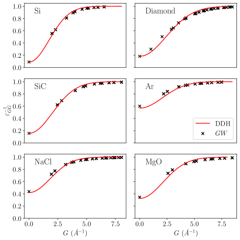
Figure 1: Inverse dielectric functions vs. wave vector at the $\Gamma$ point for Si, diamond, SiC, Ar, NaCl and MgO, as calculated in $GW$ and given by the model in Eq. (3) with parameters taken from Ref. Chen et al. (2018).

The excitation spectra in both BSE and TD-DFT are obtained by solving an eigenvalue problem, referred to as the Bethe-Salpeter and Casida equation, respectively Onida et al. (2002); Sander and Kresse (2017):

$$\begin{pmatrix}\mathbf{A}&\mathbf{B}\\ \mathbf{B^{*}}&\mathbf{A^{*}}\\ \end{pmatrix}\begin{pmatrix}\mathbf{X}\\ \mathbf{Y}\\ \end{pmatrix}=\Omega\begin{pmatrix}\mathbb{1}&0\\ 0&\mathbb{-1}\\ \end{pmatrix}\begin{pmatrix}\mathbf{X}\\ \mathbf{Y}\\ \end{pmatrix},$$ (4)

where submatrices $\mathbf{A}$ and $\mathbf{B}$ read

$$A_{ai,bj}=(\epsilon_{a}-\epsilon_{i})\delta_{i,j}\delta_{a,b}+\bra{ib}K\ket{aj},$$ (5)

$$B_{ai,bj}=\bra{ij}K\ket{ab},$$ (6)

with the indices $i,j$ and $a,b$ referring to occupied and unoccupied states, respectively. The excitation frequencies of the system are given by $\Omega$. $X$ and $Y$ are the two-body electron-hole eigenstates in the transition basis $\psi_{a}(\mathbf{r})\psi_{i}^{*}(\mathbf{r^{\prime}})$ and $\psi_{i}(\mathbf{r})\psi_{a}^{*}(\mathbf{r^{\prime}})$. Matrix $A$ includes two terms, the energy of the direct transition from occupied to unoccupied states and the electron-hole interaction described by the kernel $K$ Strinati (1984); Rohlfing and Louie (1998b). Equation (4) is non-Hermitian, which makes it difficult to solve with standard eigenvalue solvers Sander et al. (2015); Maggio and Kresse (2016). A common practice to avoid this difficulty is to neglect the coupling between excitations and de-excitations by setting $B$ to zero. This approximation is known as the Tamm-Dancoff approximation.

The distinction between BSE-$GW$ and TD-DFT approaches results, on the one hand, from the origin of the one-particle eigenfunctions and energies and, on the other hand, from the type of the interaction kernel $K$. To make the comparison between different methods more transparent, we provide in Fig. 2 the Feynman diagrams corresponding to the various irreducible polarizabilities $\tilde{\chi}$ discussed in this work.

Figure 2: Irreducible polarizabilities $\tilde{\chi}$ in various approximations. The reducible polarizability is obtained from $\chi=\tilde{\chi}+\tilde{\chi}v\chi$. The wiggly line indicates the screened interaction $W$.

In BSE-$GW$, the orbitals and energies are derived from a preceding $GW$ calculation and the kernel consists of a Hartree term $V$ and a screened exchange term $W$Rohlfing and Louie (1998b):

$$\bra{ib}K\ket{aj}=2\bra{ib}V\ket{aj}-\bra{ib}W\ket{ja}.$$ (7)

The Hartree term describes the bare Coulomb interaction and is the same in all the approximations considered here. It can be included straightforwardly in a two-point formulation involving the polarizability $\chi$. The exchange term, however, requires calculating four-point integrals, which drastically increases the complexity of the problem. The screening of the exchange interaction is determined by the frequency-dependent dielectric function $\epsilon$ obtained from $GW$ and is represented by a vertical wiggly line in the diagrams. However, as shown in Refs. Rohlfing and Louie (2000); Bechstedt et al. (1997); Marini and Del Sole (2003), the dynamical effects can often be neglected in BSE calculations.

In the TD-DFT approach, the electron energies and wave functions are obtained from a semilocal or hybrid-functional calculation. The interaction kernel consists of three terms, a Hartree and a screened exchange term $W^{\rm m}$ like in the BSE, and an additional local exchange-correlation interaction $f^{\textrm{loc}}_{\textrm{xc}}$Casida and Huix-Rotllant (2012):

$$\bra{ib}K\ket{aj}=2\bra{ib}V\ket{aj}-\bra{ib}W^{\rm m}\ket{ja}+\bra{ib}f^{\textrm{loc}}_{\textrm{xc}}\ket{aj}.$$ (8)

The screening of the exchange interaction in TD-DFT is described by a constant through $W^{\rm m}=c_{\rm x}V(|\mathbf{q+G}|)$ or by a function through $W^{\rm m}=c_{\text{x}}(\left|\mathbf{q+G}\right|)V(|\mathbf{q+G}|)$, depending on the exchange-correlation functional. In particular, $c_{\text{x}}=0$ for semilocal DFT functionals. In the case of DDH, the exchange interaction is screened by the model inverse dielectric function $c_{\text{x}}=c^{\text{DDH}}_{\text{x}}(\left|\mathbf{q+G}\right|)$ given in Eq. (3) and the local exchange-correlation interaction $f^{\textrm{loc}}_{\textrm{xc}}$ is derived from the local part of the exchange-correlation potential

$$f_{\textrm{xc}}^{\textrm{loc}}(\mathbf{r,r^{\prime}})=\frac{\delta\left\{V_{c}^{\textrm{PBE}}+\left(1-\epsilon^{-1}_{\infty}\right)V_{x}^{\textrm{PBE,LR}}\right\}}{\delta\rho(\mathbf{r})}\delta(\mathbf{r-r^{\prime}}).$$ (9)

In Fig. 2$,f^{\textrm{loc}}_{\textrm{xc}}$ is represented by a dotted line connecting $\chi_{0}$ and $\tilde{\chi}$. In this work, we refer to this version of TD-DFT as TD-DDH.

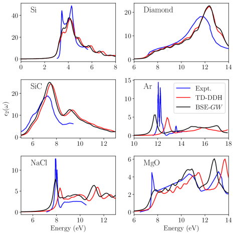
Figure 3: Absorption spectra for Si, diamond, SiC, Ar, NaCl and MgO calculated with BSE-$GW$ and TD-DDH. Experimentally measured spectra are taken from Palik (2012) for diamond, from Logothetidis et al. (1986) for Si, from Logothetidis and Petalas (1996) for SiC, from Saile et al. (1976) for Ar, from Roessler and Walker (1968) for NaCl, and from Bortz et al. (1990) for MgO.

Next, we focus on the comparison between BSE-$GW$ and TD-DDH. In both schemes, the absorption spectra are obtained from the eigenvalue problem in Eq. (4). In particular, the BSE-$GW$ calculations are based on partially self-consistent $GW$ using the “nanoquanta” vertex corrections $f_{\rm xc}$ in the polarizability $\tilde{\chi}$ Not . These two approaches are tested on a set of materials possessing a wide range of band gaps. The corresponding spectra are given in Fig. 3. Our calculations show that both approaches agree well with experiment and that TD-DDH reproduces all the spectral features with the correct oscillator strengths. In the case of diamond, Si and SiC, the spectra are nearly on top of each other. For Ar, NaCl, and MgO, the relative positions of the main features in the spectra are found to be shifted slightly. In principle, this shift can result from differences in the band structure and in the screening. Our analysis indicates that the dominant effect is due to the energy transition terms in Eq. (5). From Table 1, we notice that the calculated band gaps differ by less than 0.15 eV for Si, SiC, and diamond, but that the disagreement is more substantial for NaCl, Ar, and MgO. Overall, when compared to experimental values corrected for the coupling to phonons, DDH and $GW$ band gaps show mean average errors of 0.11 and 0.22 eV, respectively. These errors are consistent with the current accuracy of ab initio methods Shishkin et al. (2007); Chen and Pasquarello (2015), indicating that the agreement with experiment should be considered excellent for both schemes. As far as the screening is concerned, we show below that the small discrepancies observed in Fig. 1 hardly change the spectra.

The performance of TD-DDH can also be assessed through a comparison with TD-PBE0, an approach commonly used for the calculations of spectra Vörös and Gali (2009); Yang et al. (2015). TD-PBE0 is based on a global hybrid functional where 25% of Fock exchange is used uniformly and the exchange interaction in the calculation of the spectra is screened by $\varepsilon_{\infty}$. As shown in the SM Sup , the accuracy of TD-DDH is significantly better. Moreover, TD-PBE0 does not reproduce the dielectric screening over the full range, which obscures the understanding of the underlying physics.

Table 1: Band gaps (in eV) obtained with the semilocal PBE functional Perdew et al. (1996), DDH, and $GW$. The experimental values are augmented by theoretical corrections resulting from the coupling to phonons.

	Si	SiC	Diamond		NaCl	Ar	MgO
PBE	0.75	1.35	4.14		5.21	8.70	4.77
DDH	1.31	2.50	5.69		9.13	14.60	8.41
$GW$	1.41	2.55	5.85		8.86	13.75	8.12
Expt.	1.23	2.53	5.85		9.14	14.33	8.36

To compare the screening in BSE-$GW$ and TD-DDH, we show in Fig. 4 the absorption spectra of diamond calculated in various approximations using the same energies and wave functions, which are taken from a $G_{0}W_{0}$ calculation. We start our analysis from a BSE calculation in which the full static inverse dielectric matrix is used ($W^{\rm full}$). In particular, we show that the off-diagonal elements of this matrix barely have any effect on the calculated spectrum ($W^{\rm diag}$), in accordance with Ref. Sun et al. (2020). Next, we replace the inverse dielectric function with the model $c^{\text{DDH}}_{\text{x}}\left(\left|\mathbf{q+G}\right|\right)$ and find no discernible difference in the spectrum ($W^{\rm m}$). Notice that we here consider isotropic screening and that the extension of this model to anisotropic materials remains to be investigated. The present treatment of the screening is equivalent to that of TD-DDH, where the local exchange-correlation kernel is neglected, i.e. $f^{\textrm{loc}}_{\textrm{xc}}=0$, also referred to as model BSE (mBSE) Bokdam et al. (2016); Sun et al. (2020). To restore the full TD-DDH screening, we include the $f^{\textrm{loc}}_{\textrm{xc}}$ and still obtain essentially the same spectrum ($W^{\rm m}+f^{\textrm{loc}}_{\textrm{xc}}$). Hence, these results indicate that the model screening in TD-DDH gives an accurate description of the screening in $W=\epsilon^{-1}V$ and that the effect of $f^{\textrm{loc}}_{\textrm{xc}}$ is negligible for extended systems. Considering this, we can say that for extended systems TD-DDH is de facto equivalent to mBSE.

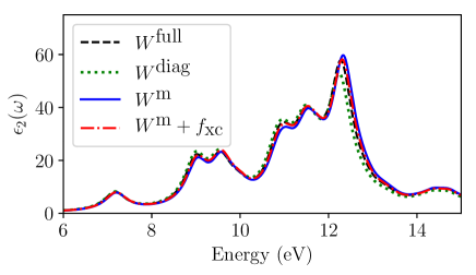
Figure 4: Optical absorption spectrum of diamond calculated with BSE and full $\epsilon^{-1}$ from $GW$ ($W^{\mathrm{full}}$), BSE and diagonal $\epsilon^{-1}$ ($W^{\mathrm{diag}}$), BSE and model $\epsilon^{-1}_{\textrm{model}}$ ($W^{\textrm{m}}$), TD-DDH and model $\epsilon^{-1}_{\textrm{model}}$ with $f^{\textrm{loc}}_{\textrm{xc}}$ ($W^{\textrm{m}}+f^{\textrm{loc}}_{\textrm{xc}}$). All spectra are based on energies and wave functions from a $G_{0}W_{0}$ calculation. A $6\times 6\times 6$ k-point grid is used.

The numerical complexity of Eq. (4) is the same in BSE and TD-DDH. However, the preceding $GW$ calculations required in BSE-$GW$ involve a high computational cost, which scales like $N^{4}$ in the number of electrons $N$ in most $GW$ implementations instead of like $N^{3}$ in TD-DFT. Additionally, in the calculation of the Green’s function in $GW$, the convergence with respect to the number of unoccupied states and the number of frequency points has to be controlled carefully, which significantly increases the complexity of the calculations. Note that the static dielectric constant only needs to be determined at the $\Gamma$ point of the Brillouin zone and that it converges quickly with respect to the number of included orbitals. Furthermore, the hybrid-functional approach only requires a model static dielectric function, for which the static limit can be obtained rather efficiently Cui et al. (2018). Thus, the hybrid functional approach opens the way to more efficient numerical schemes that can circumvent the calculation of the full dielectric matrix.

In conclusion, we have shown that time-dependent calculations using the parameter-free DDH functional yield optical absorption spectra with an accuracy comparable to BSE-$GW$. The success of this approach originates from the use of a model dielectric function that gives a physically motivated description of the screened exchange interaction over the full spatial range. Notably, the computational complexity of the method is drastically reduced compared to BSE-$GW$, as it eliminates the need for preceding $GW$ calculations. This will allow one to consider larger and more complex systems than hitherto possible.

The structures and the input files used for the calcula- tions are freely available on the Materials Cloud platform, see Ref. Clo .

Support from the Swiss National Science foundation is acknowledged under Grant No. 200020-172524. The calculations have been performed at the Swiss National Supercomputing Centre (CSCS) (grant under project ID s879) and at SCITAS-EPFL.

References

- Perdew and Levy (1983) J. P. Perdew and M. Levy, Phys. Rev. Lett. 51, 1884 (1983).
- Sham and Schlüter (1983) L. J. Sham and M. Schlüter, Phys. Rev. Lett. 51, 1888 (1983).
- Hedin (1965) L. Hedin, Phys. Rev. 139, A796 (1965).
- Hedin and Lundqvist (1970) L. Hedin and S. Lundqvist, in Solid State Phys., Solid State Physics, Vol. 23, edited by F. Seitz, D. Turnbull, and H. Ehrenreich (Academic Press, 1970) pp. 1–181.
- Hybertsen and Louie (1985) M. S. Hybertsen and S. G. Louie, Phys. Rev. Lett. 55, 1418 (1985).
- Aryasetiawan and Gunnarsson (1998) F. Aryasetiawan and O. Gunnarsson, Reports Prog. Phys. 61, 237 (1998).
- Onida et al. (2002) G. Onida, L. Reining, and A. Rubio, Rev. Mod. Phys. 74, 601 (2002).
- Albrecht et al. (1998) S. Albrecht, L. Reining, R. Del Sole, and G. Onida, Phys. Rev. Lett. 80, 4510 (1998).
- Benedict et al. (1998) L. X. Benedict, E. L. Shirley, and R. B. Bohn, Phys. Rev. Lett. 80, 4514 (1998).
- Rohlfing and Louie (1998a) M. Rohlfing and S. G. Louie, Phys. Rev. Lett. 80, 3320 (1998a).
- Hanke and Sham (1980) W. Hanke and L. J. Sham, Phys. Rev. B 21, 4656 (1980).
- Gross and Kohn (1985) E. K. U. Gross and W. Kohn, Phys. Rev. Lett. 55, 2850 (1985).
- Runge and Gross (1984) E. Runge and E. K. U. Gross, Phys. Rev. Lett. 52, 997 (1984).
- Casida (1995) M. E. Casida, in Recent Adv. Density-Functional Methods, edited by D. P. Chong (World Scientific, Singapore, 1995) part i ed.
- Vasiliev et al. (1999) I. Vasiliev, S. Ögüt, and J. R. Chelikowsky, Phys. Rev. Lett. 82, 1919 (1999).
- Rubio et al. (1996) A. Rubio, J. A. Alonso, X. Blase, L. C. Balbás, and S. G. Louie, Phys. Rev. Lett., Tech. Rep. 2 (1996).
- Gavrilenko and Bechstedt (1996) V. I. Gavrilenko and F. Bechstedt, Phys. Rev. B 54, 13416 (1996).
- Sottile et al. (2003) F. Sottile, V. Olevano, and L. Reining, Phys. Rev. Lett. 91, 056402 (2003).
- Marini et al. (2003) A. Marini, R. Del Sole, and A. Rubio, Phys. Rev. Lett. 91, 256402 (2003).
- Adragna et al. (2003) G. Adragna, R. Del Sole, and A. Marini, Phys. Rev. B 68, 165108 (2003).
- Salzner et al. (1997) U. Salzner, J. B. Lagowski, P. G. Pickup, and R. A. Poirier, J. Comput. Chem. 18, 1943 (1997).
- Laurent and Jacquemin (2013) A. D. Laurent and D. Jacquemin, “TD-DFT benchmarks: A review,” (2013).
- Bruneval et al. (2006) F. Bruneval, F. Sottile, V. Olevano, and L. Reining, J. Chem. Phys. 124, 144113 (2006).
- Botti et al. (2007) S. Botti, A. Schindlmayr, R. Del Sole, and L. Reining, Reports Prog. Phys. 70, 357 (2007).
- Paier et al. (2008) J. Paier, M. Marsman, and G. Kresse, Phys. Rev. B 78, 121201(R) (2008).
- Yang et al. (2015) Z.-H. Yang, F. Sottile, and C. A. Ullrich, Phys. Rev. B 92, 035202(R) (2015).
- Refaely-Abramson et al. (2015) S. Refaely-Abramson, M. Jain, S. Sharifzadeh, J. B. Neaton, and L. Kronik, Phys. Rev. B 92, 081204(R) (2015).
- Elliott et al. (2019) J. D. Elliott, N. Colonna, M. Marsili, N. Marzari, and P. Umari, J. Chem. Theory Comput. 15, 3710 (2019).
- Wing et al. (2019) D. Wing, J. B. Haber, R. Noff, B. Barker, D. A. Egger, A. Ramasubramaniam, S. G. Louie, J. B. Neaton, and L. Kronik, Phys. Rev. Mater. 3, 064603 (2019).
- Sun et al. (2020) J. Sun, J. Yang, and C. A. Ullrich, Phys. Rev. Res. 2, 013091 (2020).
- Chen et al. (2018) W. Chen, G. Miceli, G. M. Rignanese, and A. Pasquarello, Phys. Rev. Mater. 2, 073803 (2018).
- Cui et al. (2018) Z. H. Cui, Y. C. Wang, M. Y. Zhang, X. Xu, and H. Jiang, J. Phys. Chem. Lett. 9, 2338 (2018).
- Liu et al. (2020) P. Liu, C. Franchini, M. Marsman, and G. Kresse, J. Phys. Condens. Matter 32, 015502 (2020).
- Perdew et al. (1996) J. P. Perdew, K. Burke, and M. Ernzerhof, Phys. Rev. Lett. 77, 3865 (1996).
- (35) See Supplemental Material for computational details, quasi-particle self-consistent (QS), and TD-PBE0 calculations.
- Sander and Kresse (2017) T. Sander and G. Kresse, J. Chem. Phys. 146, 064110 (2017).
- Strinati (1984) G. Strinati, Phys. Rev. B 29, 5718 (1984).
- Rohlfing and Louie (1998b) M. Rohlfing and S. G. Louie, Phys. Rev. Lett. 81, 2312 (1998b).
- Sander et al. (2015) T. Sander, E. Maggio, and G. Kresse, Phys. Rev. B 92, 045209 (2015).
- Maggio and Kresse (2016) E. Maggio and G. Kresse, Phys. Rev. B 93, 235113 (2016).
- Rohlfing and Louie (2000) M. Rohlfing and S. G. Louie, Phys. Rev. B 62, 4927 (2000).
- Bechstedt et al. (1997) F. Bechstedt, K. Tenelsen, B. Adolph, and R. Del Sole, Phys. Rev. Lett. 78, 1528 (1997).
- Marini and Del Sole (2003) A. Marini and R. Del Sole, Phys. Rev. Lett. 91, 176402 (2003).
- Casida and Huix-Rotllant (2012) M. Casida and M. Huix-Rotllant, Annu. Rev. Phys. Chem. 63, 287 (2012).
- Palik (2012) E. D. Palik, Handb. Opt. Constants Solids, Vol. 1 (Academic Press, 2012) pp. 1–804.
- Logothetidis et al. (1986) S. Logothetidis, P. Lautenschlager, and M. Cardona, Phys. Rev. B 33, 1110 (1986).
- Logothetidis and Petalas (1996) S. Logothetidis and J. Petalas, J. Appl. Phys. 80, 1768 (1996).
- Saile et al. (1976) V. Saile, M. Skibowski, W. Steinmann, P. Gürtler, E. E. Koch, and A. Kozevnikov, Phys. Rev. Lett. 37, 305 (1976).
- Roessler and Walker (1968) D. M. Roessler and W. C. Walker, Phys. Rev. 166, 599 (1968).
- Bortz et al. (1990) M. L. Bortz, R. H. French, D. J. Jones, R. V. Kasowski, and F. S. Ohuchi, Phys. Scr., Tech. Rep. (1990).
- (51) Fully self-consistent as in QS does not lead to appreciable differences in the spectra Sup .
- Shishkin et al. (2007) M. Shishkin, M. Marsman, and G. Kresse, Phys. Rev. Lett. 99, 246403 (2007).
- Chen and Pasquarello (2015) W. Chen and A. Pasquarello, Phys. Rev. B 92, 041115(R) (2015).
- Vörös and Gali (2009) M. Vörös and A. Gali, Phys. Rev. B 80, 161411(R) (2009).
- Bludau et al. (1974) W. Bludau, A. Onton, and W. Heinke, J. Appl. Phys. 45, 1846 (1974).
- Cardona and Thewalt (2005) M. Cardona and M. L. Thewalt, Rev. Mod. Phys. 77, 1173 (2005).
- Humphreys et al. (1981) R. G. Humphreys, D. Bimberg, and W. J. Choyke, Solid State Commun. 39, 163 (1981).
- Monserrat and Needs (2014) B. Monserrat and R. J. Needs, Phys. Rev. B 89, 214304 (2014).
- Clark et al. (1964) C. D. Clark, P. J. Dean, P. V. Harris, and W. C. Price, Proc. R. Soc. London. Ser. A. Math. Phys. Sci. 277, 312 (1964).
- Lambrecht et al. (2017) W. R. L. Lambrecht, C. Bhandari, and M. van Schilfgaarde, Phys. Rev. Mater. 1, 43802 (2017).
- Baldini (1962) G. Baldini, Phys. Rev. 128, 1562 (1962).
- Zacharias and Giustino (2016) M. Zacharias and F. Giustino, Phys. Rev. B 94, 075125 (2016).
- Karsai et al. (2018) F. Karsai, M. Engel, E. Flage-Larsen, and G. Kresse, New J. Phys. 20, 123008 (2018).
- Hinuma et al. (2014) Y. Hinuma, A. Grüneis, G. Kresse, and F. Oba, Phys. Rev. B 90, 155405 (2014).
- Nery et al. (2018) J. P. Nery, P. B. Allen, G. Antonius, L. Reining, A. Miglio, and X. Gonze, Phys. Rev. B 97, 115145 (2018).
- Bokdam et al. (2016) M. Bokdam, T. Sander, A. Stroppa, S. Picozzi, D. D. Sarma, C. Franchini, and G. Kresse, Sci. Rep. (2016).
- (67) 10.24435/materialscloud:gn-2p.