Numerical verification for asymmetric solutions of the Hénon equation on bounded domains

Abstract

The Hénon equation, a generalized form of the Emden equation, admits symmetry-breaking bifurcation for a certain ratio of the transverse velocity to the radial velocity. Therefore, it has asymmetric solutions on a symmetric domain even though the Emden equation has no asymmetric unidirectional solution on such a domain. We discuss a numerical verification method for proving the existence of solutions of the Hénon equation on a bounded domain. By applying the method to a line-segment domain and a square domain, we numerically prove the existence of solutions of the Hénon equation for several parameters representing the ratio of transverse to radial velocity. As a result, we find a set of undiscovered solutions with three peaks on the square domain.

1 Introduction

The Hénon equation was proposed as a model for mass distribution in spherically symmetric star clusters, which is important in studying the stability of rotating stars [1]. One important aspect of the model is the Dirichlet boundary value problem

$$\begin{cases}-\Delta u=|\boldsymbol{x}-\boldsymbol{x_{0}}|^{l}|u|^{p-1}u&{\rm in}\quad\Omega,\\ u=0&{\rm on}\quad\partial\Omega,\end{cases}$$ (1)

where $\Omega\subset\mathbb{R}^{N}(N=1,2,3)$ is a bounded domain, $\boldsymbol{x}$ is the location of the star, and $u$ stands for the stellar density. Particularly, $\boldsymbol{x_{0}}$ is set at the center of the domain. The parameter $2\leq p<p^{*}$ ($p^{*}=\infty$ if $N=1,2$ and $p^{*}=5$ if $N=3$) is the polytropic index, determined according to the central density of each stellar type. The parameter $l\geq 0$ is the ratio of the transverse velocity to the radial velocity. These velocities can be derived by decomposing the space velocity vector into the radial and transverse components.

When $l=0$, the Hénon equation coincides with the Emden equation $-\Delta u=|u|^{p-1}u\text{ in }\Omega$. In this case, the transverse velocity vanishes and the orbit becomes purely radial. Gidas, Ni, and Nirenberg proved that the Emden equation has no asymmetric unidirectional solution in a rectangle domain [2]. However, Breuer, Plum, and McKenna reported some asymmetric solutions obtained with an approximate computation based on the Galerkin method [3], which were called “spurious approximate solutions” caused by discretization errors. This example shows the need to verify approximate computations. By contrast, a theoretical analysis [4] for large $l$ (when the orbit tends to be purely circular) found that the Hénon equation admits symmetry-breaking bifurcation, thereby having several asymmetric solutions even on a symmetric domain.

The importance of the Hénon equation has led to active mathematical study on it over the last decade. For example, Amadori and Gladiali [5] analyzed the bifurcation structure of (1) with respect to parameter $p$. They applied an analytical method to the Hénon equation that had worked for the Emden equation. Additionally, several numerical studies have been conducted on the Hénon equation [6, 7, 8, 9]. In particular, we are motivated by the work of Yang, Li, and Zhu [6], who developed an effective computational method to find multiple asymmetric solutions of (1) on the unit square $\Omega=(0,1)^{2}$ using algorithms based on the bifurcation method. They generated the bifurcation curve of (1) with $p=3$ and numerically predicted bifurcation points around $l=0.5886933$ and $l=2.3654862$ using approximate computations.

The purpose of our study is to prove the existence of solutions of (1) using the Newton–Kantorovich theorem (see Theorem 2). We prove their existence through the following steps:

1. We construct approximate solutions $\hat{u}$ using the Galerkin method with polynomial approximations.

2. Using the Newton–Kantorovich theorem (Theorem 3), we prove the existence of solutions $u$ of (1) with nearby approximations $\hat{u}$ while sharply evaluating the error bound between $u$ and $\hat{u}$ in terms of the $H^{1}_{0}$-norm $\|\nabla\cdot\|_{L^{2}}$.

By applying the above steps to the problem (1) on the domains $\Omega=(0,1)^{N}$ $(N=1,2)$, we successfully prove the existence of several solutions for $l=0,2,4$. In particular, we find a set of solutions with three peaks, which were not revealed in [6] (see Figure 2).

The remainder of this paper is organized as follows. Some notation is introduced in Section 2. Sections 3 and 4 describe numerical verification based on the Newton–Kantorovich theorem together with evaluations of several required constants. Section 5 shows the results numerically proving the existence of several asymmetric solutions of (1). Subsequently, we discuss the solution curves of the problem for $p=3$ based on an approximate computation.

2 Preliminaries

We begin by introducing some notation. For two Banach spaces $X$ and $Y$, the set of bounded linear operators from $X$ to $Y$ is denoted by $\mathcal{L}(X,Y)$. The norm of $T\in\mathcal{L}(X,Y)$ is defined by

$$\|T\|_{\mathcal{L}(X,Y)}:=\sup_{0\neq u\in X}\frac{\|Tu\|_{Y}}{\|u\|_{X}}.$$ (2)

Let $L^{p}(\Omega)$ $(1\leq p<\infty)$ be the function space of $p$-th power Lebesgue integrable functions over a domain $\Omega$ with the $L^{p}$-norm $\|u\|_{L^{p}}:=\left(\int_{\Omega}|u(x)|^{p}dx\right)^{1/p}<\infty.$ When $p=2$, $L^{2}(\Omega)$ is the Hilbert space with the inner product $(u,v)_{L^{2}}:=\int_{\Omega}u(x)v(x)dx$. Let $L^{\infty}(\Omega)$ be the function space of Lebesgue measurable functions over $\Omega$, with the norm $\|u\|_{L^{\infty}}:=\operatorname{ess}\sup\{|u(x)|:x\in\Omega\}\text{ for }u\in L^{\infty}(\Omega)$. We denote the first-order $L^{2}$ Sobolev space in $\Omega$ as $H^{1}(\Omega)$ and define

$$H_{0}^{1}(\Omega):=\left\{u\in H^{1}(\Omega):u=0\text{ on }\partial\Omega\text{ in the trace sense}\right\}$$

as the solution space for the target equation (1). We endow $H^{1}_{0}(\Omega)$ with the inner product and norm

$$(u,v)_{H^{1}_{0}}: =(\nabla u,\nabla v)_{L^{2}}+\tau(u,v)_{L^{2}},\quad u,v\in H^{1}_{0}(\Omega),$$ (3)

$$\|u\|_{H^{1}_{0}}: =\sqrt{(u,u)_{H^{1}_{0}}},\quad u\in H^{1}_{0}(\Omega),$$ (4)

where $\tau$ is a nonnegative number chosen as

$$\tau>-p|\boldsymbol{x}-\boldsymbol{x_{0}}|^{l}|\hat{u}(\boldsymbol{x})|^{p-1}\text{~{}~{}a.e.~{}~{}}\boldsymbol{x}\in\Omega$$ (5)

for a numerically computed approximation $\hat{u}\in H^{1}_{0}(\Omega)$. The condition (5) is required in Subsection 4.2 and $\hat{u}$ is explicitly constructed in Section 5. Because the norm $\|\cdot\|_{H^{1}_{0}}$ monotonically increases with respect to $\tau$, the $H^{1}_{0}(\Omega)$ norm $\|\nabla\cdot\|_{L^{2}}$ is dominated by the norm $\|\cdot\|_{H^{1}_{0}}$ for all $\tau\geq 0$. Therefore, the error bound $\|u-\hat{u}\|_{H^{1}_{0}}$ is always an upper bound for $\|\nabla(u-\hat{u})\|_{L^{2}}$. The topological dual space of $H^{1}_{0}(\Omega)$ is denoted by $H^{-1}$ with the usual supremum norm defined in (2).

The bound for the embedding $H^{1}_{0}(\Omega)\hookrightarrow L^{p}(\Omega)$ is denoted by $C_{p}$ $(p\geq 2)$. More precisely, $C_{p}$ is a positive number satisfying

$$\|u\|_{L^{p}}\leq C_{p}\|u\|_{H^{1}_{0}}\quad\text{ for all }u\in H^{1}_{0}(\Omega).$$ (6)

Note that $\|u\|_{H^{-1}}\leq C_{p}\|u\|_{L^{p^{\prime}}}$, $u\in L^{p^{\prime}}(\Omega)$ holds for $p^{\prime}$ satisfying $p^{-1}+p^{\prime-1}=1$ . Explicitly estimating the embedding constant $C_{p}$ is important for our numerical verification. When $p=2$, we use the following optimal inequality:

$$\|u\|_{L^{2}}\leq\frac{1}{\sqrt{\lambda_{1}+\tau}}\|u\|_{H^{1}_{0}},$$

where $\lambda_{1}$ is the first eigenvalue of the minus Laplacian in the weak sense. Especially when $\Omega=(0,1)^{N}$, we have $\lambda_{1}=N\pi^{2}$. When $p$ is not $2$, we use the following theorems depending on the dimension of $\Omega$. We use [10, Lemma 7.12] to obtain an explicit value of $C_{p}$ for a one-dimensional bounded domain.

Theorem 1 ([10, Lemma 7.12]).

Let $\Omega=(a,b)\subset\mathbb{R}$, with $a\in\mathbb{R}\cup\{-\infty\}$, $b\in\mathbb{R}\cup\{+\infty\}$, $a<b$. Moreover, let $\rho^{*}$ denote the minimal point of the spectrum of $-u^{\prime\prime}$ on $H^{1}_{0}(\Omega)$, i.e. $\rho^{*}=\pi^{2}/(b-a)^{2}$ if $(a,b)$ is bounded. Then, for all $u\in H_{0}^{1}(\Omega)$,

$$\|u\|_{L^{p}}\leq C_{p}\|u\|_{H_{0}^{1}}\quad(p\in(2,\infty)),$$

where, abbreviating $\varepsilon:=\frac{2}{p}\in(0,1)$,

$$C_{p}:=\begin{cases}\frac{1}{\sqrt{2}}(1-\varepsilon)^{\frac{1}{4}(1-\varepsilon)}(1+\varepsilon)^{\frac{1}{4}(1+\varepsilon)}\tau^{-\frac{1}{4}(1+\varepsilon)}&\text{ if }\quad\rho^{*}\leq\tau\frac{1-\varepsilon}{1+\varepsilon},\\ \frac{1}{\sqrt{\rho^{*}+\tau}}\left(\rho^{*}\right)^{\frac{1}{4}(1-\varepsilon)}&\text{ otherwise },\end{cases}$$

for $p\in(2,\infty)$.

When $N\geq 2$, we use [11, Corollary A.2] or [10, Lemma 7.10] to obtain $C_{p}$ for bounded domains $\Omega\subset\mathbb{R}^{N}$. In our numerical experiments in Section 5, $C_{p}$ evaluated by [11, Corollary A.2] is smaller than that evaluated by [10, Lemma 7.10].

Theorem 2 ([11, Corollary A.2]).

Let $\Omega\subset\mathbb{R}^{N}(N\geq 2)$ be a bounded domain, the measure of which is denoted by $|\Omega|$. Let $p\in(N/(N-1),2N/(N-2)]$ if $N\geq 3$, $p\in(2,\infty)$ if $N=2$. We set $q=Np/(N+p)$. Then, (6) holds for

$$C_{p}(\Omega)=|\Omega|^{\frac{2-q}{2q}}T_{p}.$$

Here, $T_{p}$ is defined by

$$T_{p}=\pi^{-\frac{1}{2}}N^{-\frac{1}{q}}\left(\frac{q-1}{N-q}\right)^{1-\frac{1}{q}}\left\{\frac{\Gamma\left(1+\frac{N}{2}\right)\Gamma(N)}{\Gamma\left(\frac{N}{q}\right)\Gamma\left(1+N-\frac{N}{q}\right)}\right\}^{\frac{1}{N}},$$

where $\Gamma$ is the gamma function.

3 Numerical verification method

This section discusses the numerical verification method used in this paper. We first define the operator $f$ as

$$f:\begin{cases}u(\cdot)&\mapsto|\boldsymbol{\cdot}-\boldsymbol{x_{0}}|^{l}|u(\cdot)|^{p-1}u(\cdot),\\ H^{1}_{0}(\Omega)&\to H^{-1},\end{cases}$$

where $2\leq p<p^{*}$ ($p^{*}=\infty$ if $N=1,2$ and $p^{*}=5$ if $N=3$). Furthermore, we define the nonlinear operator $F:H^{1}_{0}(\Omega)\rightarrow H^{-1}$ by $F(u):=-\Delta u-f(u)$, which is given by

$$\langle F(u),v\rangle=(\nabla u,\nabla v)_{L^{2}}-\langle f(u),v\rangle\quad\text{for all}\quad v\in H^{1}_{0}(\Omega),$$

where $\langle f(u),v\rangle=\int_{\Omega}(|\boldsymbol{x}-\boldsymbol{x_{0}}|^{l}|u(\boldsymbol{x})|^{p-1}u(\boldsymbol{x}))v(\boldsymbol{x})d\boldsymbol{x}$. The Fréchet derivatives of $f$ and $F$ at $\varphi\in H^{1}_{0}(\Omega)$ are denoted by $f^{\prime}_{\varphi}$ and $F^{\prime}_{\varphi}$, respectively, and given by

$$\left\langle f_{\varphi}^{\prime}u,v\right\rangle =\int_{\Omega}(p|\boldsymbol{x}-\boldsymbol{x_{0}}|^{l}|\varphi(\boldsymbol{x})|^{p-1})u(\boldsymbol{x})v(\boldsymbol{x})d\boldsymbol{x}\quad\text{ for all }\quad u,v\in H^{1}_{0}(\Omega),$$ (7)

$$\left\langle{F}_{\varphi}^{\prime}u,v\right\rangle =(\nabla u,\nabla v)_{L^{2}}-\left\langle f_{\varphi}^{\prime}u,v\right\rangle\quad\text{ for all }\quad u,v\in H^{1}_{0}(\Omega).$$ (8)

Then, we consider the following problem:

$$\text{Find}\quad u\in H^{1}_{0}(\Omega)\quad\text{s.t.}\quad F(u)=0,$$ (9)

which is the weak form of the problem (1). To conduct the numerical verification for this problem, we apply the Newton–Kantorovich theorem, which enables us to prove the existence of a true solution $u$ near a numerically computed “good” approximate solution $\hat{u}$ (see, for example, [12]). Hereafter, $B(\hat{u},r)$ and $\bar{B}(\hat{u},r)$ respectively denote the open and closed balls with center approximate solution $\hat{u}$ and radius $r$ in terms of norm $\|\cdot\|_{H^{1}_{0}}$.

Theorem 3 (Newton–Kantorovich’s theorem).

Let $\hat{u}\in H^{1}_{0}(\Omega)$ be some approximate solution of $F(u)=0$. Suppose that there exists some $\alpha>0$ satisfying

$$\|F^{\prime-1}_{\hat{u}}F({\hat{u}})\|_{H^{1}_{0}}\leq\alpha.$$ (10)

Moreover, suppose that there exists some $\beta>0$ satisfying

$$\|F^{\prime-1}_{\hat{u}}(F^{\prime}_{v}-F^{\prime}_{w})\|_{\mathcal{L}({H^{1}_{0}},{H^{1}_{0}})}\leq\beta\|v-w\|_{H^{1}_{0}},\quad\text{ for all }v,w\in D,$$ (11)

where $D=B(\hat{u},2\alpha+\delta)$ is an open ball depending on the above value $\alpha>0$ for small $\delta>0$. If

$$\alpha\beta\leq\frac{1}{2},$$

then there exists a solution $u\in H^{1}_{0}(\Omega)$ of $F(u)=0$ in $\bar{B}(\hat{u},\rho)$ with

$$\rho=\frac{1-\sqrt{1-2\alpha\beta}}{\beta}.$$

Furthermore, the solution $u$ is unique in $\bar{B}(\hat{u},2\alpha)$.

4 Evaluation for $\alpha$ and $\beta$

To apply Theorem 3 to the numerical verification for problem (1), we need to explicitly evaluate $\alpha$ and $\beta$. The left side of (10) is evaluated as

$$\left\|F_{\hat{u}}^{\prime-1}F(\hat{u})\right\|_{H^{1}_{0}}\leq\left\|F^{\prime-1}_{\hat{u}}\right\|_{\mathcal{L}\left(H^{-1},{H^{1}_{0}}\right)}\|F(\hat{u})\|_{H^{-1}}.$$

Therefore, we set

$$\alpha=\left\|F^{\prime-1}_{\hat{u}}\right\|_{\mathcal{L}\left(H^{-1},{H^{1}_{0}}\right)}\|F(\hat{u})\|_{H^{-1}}.$$

Moreover, the left side of (11) is estimated as

$$\left\|F_{\hat{u}}^{\prime-1}\left(F_{v}^{\prime}-F_{w}^{\prime}\right)\right\|_{\mathcal{L}({H^{1}_{0}},{H^{1}_{0}})} \leq\left\|F_{\hat{u}}^{\prime-1}\right\|_{\mathcal{L}\left(H^{-1},{H^{1}_{0}}\right)}\left\|F_{v}^{\prime}-F_{w}^{\prime}\right\|_{\mathcal{L}\left({H^{1}_{0}},H^{-1}\right)}$$

$$=\left\|F_{\hat{u}}^{\prime-1}\right\|_{\mathcal{L}\left(H^{-1},{H^{1}_{0}}\right)}\left\|f^{\prime}_{v}-f^{\prime}_{w}\right\|_{\mathcal{L}\left({H^{1}_{0}},H^{-1}\right)}.$$

Hence, the desired value of $\beta$ is obtained via

$$\beta \leq\|F^{\prime-1}_{\hat{u}}\|_{\mathcal{L}({H^{-1}},{H^{1}_{0}})}L,$$

where $L$ is the Lipschitz constant satisfying

$$\left\|f^{\prime}_{v}-f^{\prime}_{w}\right\|_{\mathcal{L}\left({H^{1}_{0}},H^{-1}\right)}\leq L\|v-w\|_{H^{1}_{0}}\quad\text{ for all }v,w\in D.$$ (12)

We are left to evaluate the inverse operator norm $\|F^{\prime-1}_{\hat{u}}\|_{\mathcal{L}({H^{-1}},{H^{1}_{0}})}$, the residual norm $\|F({\hat{u}})\|_{H^{-1}}$, and the Lipschitz constant $L$ for problem (9).

4.1 Residual norm $\|F({\hat{u}})\|_{H^{-1}}$

If the approximation $\hat{u}$ is sufficiently smooth so that $\Delta\hat{u}\in L^{2}(\Omega)$, we can evaluate the residual norm $\|F({\hat{u}})\|_{H^{-1}}$ as follows:

$$\|F({\hat{u}})\|_{H^{-1}}\leq C_{2}\|\Delta\hat{u}+f(\hat{u})\|_{L^{2}},$$ (13)

where $C_{2}$ is the embedding constant satisfying (6) for $p=p^{\prime}=2$. Our numerical experiments discussed in Section 5 use this evaluation, calculating the $L^{2}$-norm via stable numerical integration with all rounding errors strictly estimated.

However, the condition $\Delta\hat{u}\in L^{2}(\Omega)$ is not satisfied such as when we construct $\hat{u}$ with a piecewise linear finite element basis. We use the method of [10, Subsection 7.2] to evaluate the residual norm applicable to such a case. The following is a brief description of the evaluation method. First, we find an approximation $\rho\in H(\operatorname{div},\Omega)=\left\{\tau\in L^{2}(\Omega)^{N}:\operatorname{div}\tau\in L^{2}(\Omega)\right\}$ to $\nabla\hat{u}$. Then, the residual norm is evaluated as

$$\|{F}(\hat{u})\|_{H^{-1}} =\|-\Delta\hat{u}-f(\hat{u})\|_{H^{-1}},$$

$$=\|-\Delta\hat{u}+\operatorname{div}\rho-\operatorname{div}\rho-f(\hat{u})\|_{H^{-1}},$$

$$\leq\|\operatorname{div}(-\nabla\hat{u}+\rho)\|_{H^{-1}}+\|\operatorname{div}\rho+f(\hat{u})\|_{H^{-1}},$$

$$\leq\|-\nabla\hat{u}+\rho\|_{L^{2}}+C_{2}\|\operatorname{div}\rho+f(\hat{u})\|_{L^{2}},$$

where we used $\|\mathrm{div}\omega\|_{H^{-1}}\leq\|\omega\|_{L^{2}}$ for $\omega\in H(\mathrm{div},\Omega)$. As mentioned in [10, Subsection 7.2], $\rho$ can be computed without additional computational resources when we use the mixed finite element method to construct $\hat{u}$.

4.2 Inverse operator norm $\|F^{\prime-1}_{\hat{u}}\|_{\mathcal{L}({H^{-1}},{H^{1}_{0}})}$

In this subsection, we evaluate the inverse operator norm $\|F^{\prime-1}_{\hat{u}}\|_{\mathcal{L}(H^{-1},H^{1}_{0})}$. To this end, we use the following theorem.

Theorem 4 ([13]).

Let $\Phi:{H^{1}_{0}}(\Omega)\rightarrow H^{-1}$ be the canonical isometric isomorphism; that is, $\Phi$ is given by

$$\left\langle\Phi u,v\right\rangle:=\left(u,v\right)_{H^{1}_{0}}~{}~{}~{}{\rm for}~{}u,v\in{H^{1}_{0}(\Omega)}.$$

If

$$\displaystyle\mu_{0}:=\min\left\{|\mu|\ :\ \mu\in\sigma_{p}\left(\Phi^{-1}{F}_{\hat{u}}^{\prime}\right)\cup\{1\}\right\}$$ (14)

is positive, then the inverse of ${F}_{\hat{u}}^{\prime}$ exists, and we have

$$\left\|{F}_{\hat{u}}^{\prime-1}\right\|_{\mathcal{L}(H^{-1},H^{1}_{0})}\leq\mu_{0}^{-1},$$ (15)

where $\sigma_{p}\left(\Phi^{-1}{F}_{\hat{u}}^{\prime}\right)$ denotes the point spectrum of $\Phi^{-1}{F}_{\hat{u}}^{\prime}$.

The eigenvalue problem $\Phi^{-1}{F}_{\hat{u}}^{\prime}u=\mu u$ in ${H^{1}_{0}(\Omega)}$ is equivalent to

$$\left(\nabla u,\nabla v\right)_{L^{2}}-\langle f^{\prime}_{\hat{u}}u,v\rangle=\mu\left(u,v\right)_{H^{1}_{0}}~{}~{}{\rm for~{}all}~{}v\in{H^{1}_{0}(\Omega)},$$ (16)

where $\left(u,v\right)_{H^{1}_{0}}$ denotes the inner product defined in (3) that depends on $\tau$ and $\langle f^{\prime}_{\hat{u}}u,v\rangle$ is given by (7).

We consider the operator $\mathcal{N}:=\Phi-{F}_{\hat{u}}^{\prime}$ from $H^{1}_{0}(\Omega)$ to $H^{-1}$, which satisfies $\langle\mathcal{N}u,v\rangle=\int_{\Omega}(p|\boldsymbol{x}-\boldsymbol{x_{0}}|^{l}|\hat{u}(\boldsymbol{x})|^{p-1})u(\boldsymbol{x})v(\boldsymbol{x})d\boldsymbol{x}$ for all $u,v\in H^{1}_{0}(\Omega)$. Because $\mathcal{N}$ maps $H^{1}_{0}(\Omega)$ into $L^{2}(\Omega)$ and the embedding $L^{2}(\Omega)\hookrightarrow H^{-1}$ is compact, $\mathcal{N}:H^{1}_{0}(\Omega)\to H^{-1}$ is a compact operator. Therefore, $F^{\prime}_{\hat{u}}$ is a Fredholm operator, and the spectrum $\sigma\left(\Phi^{-1}{F}_{\hat{u}}^{\prime}\right)$ of $\Phi^{-1}{F}_{\hat{u}}^{\prime}$ is given by

$$\sigma\left(\Phi^{-1}F_{\hat{u}}^{\prime}\right)=1-\sigma\left(\Phi^{-1}\mathcal{N}\right)=1-\left\{\sigma_{p}\left(\Phi^{-1}\mathcal{N}\right)\cup\{0\}\right\}=\sigma_{p}\left(\Phi^{-1}F_{\hat{u}}^{\prime}\right)\cup\{1\}.$$

Accordingly, it suffices to look for eigenvalues $\mu\neq 1$. By setting $\lambda=(1-\mu)^{-1}$, we further transform this eigenvalue problem into

$${\rm Find}~{}u\in H^{1}_{0}(\Omega)~{}{\rm and}~{}\lambda\in\mathbb{R}~{}{\rm s.t.}~{}(u,v)_{H^{1}_{0}}=\lambda\langle(\tau+f^{\prime}_{\hat{u}})u,v\rangle~{}~{}{\rm for~{}all}~{}v\in{H^{1}_{0}(\Omega)},$$ (17)

where $\langle(\tau+f^{\prime}_{\hat{u}})u,v\rangle=\int_{\Omega}(\tau+p|\boldsymbol{x}-\boldsymbol{x_{0}}|^{l}|\hat{u}(\boldsymbol{x})|^{p-1})u(\boldsymbol{x})v(\boldsymbol{x})d\boldsymbol{x}$ for $u,v\in H^{1}_{0}(\Omega)$. Because $\tau$ is chosen so that $\tau+f^{\prime}_{\hat{u}}$ becomes positive (see (5)), (17) is a regular eigenvalue problem, the spectrum of which consists of a sequence $\{\lambda_{k}\}_{k=1}^{\infty}$ of eigenvalues converging to $+\infty$. To compute $\|F^{\prime-1}_{\hat{u}}\|_{\mathcal{L}({H^{-1}},{H^{1}_{0}})}$ on the basis of Theorem 4, we need to enclose the eigenvalue $\lambda$ of (17) that minimizes the corresponding absolute value of $|\mu|\left(=|1-\lambda^{-1}|\right)$. We consider the approximate eigenvalue problem

$${\rm Find}~{}u_{M}\in V_{M}~{}{\rm and}~{}\lambda^{M}\in\mathbb{R}~{}{\rm s.t.}\left(u_{M},v_{M}\right)_{H^{1}_{0}}=\lambda^{M}\langle(\tau+f^{\prime}_{\hat{u}})u_{M},v_{M}\rangle~{}~{}{\rm for~{}all}~{}v_{M}\in V_{M},$$ (18)

where $V_{M}$ is a finite-dimensional subspace of ${H^{1}_{0}(\Omega)}$ such as the space spanned by the finite element basis and Fourier basis. For our problem, $V_{M}$ will be explicitly chosen in Section 5. Note that (18) is a matrix problem with eigenvalues that can be enclosed with rigorous computation techniques (see, for example, [14, 15, 16]).

We then estimate the error between the $k$-th eigenvalue $\lambda_{k}$ of (17) and the $k$-th eigenvalue $\lambda_{k}^{M}$ of (18). We consider the weak formulation of the Poisson equation,

$$\left(u_{g},v\right)_{H^{1}_{0}}=\left(g,v\right)_{L^{2}}~{}~{}~{}{\rm for~{}all}~{}v\in H^{1}_{0}(\Omega)$$ (19)

given $g\in L^{2}\left(\Omega\right)$. This equation has a unique solution $u_{g}\in{H^{1}_{0}(\Omega)}$ for each $g\in L^{2}\left(\Omega\right)$ [17]. Let $P^{\tau}_{M}:{H^{1}_{0}(\Omega)}\rightarrow V_{M}$ be the orthogonal projection defined by

$$\left(P^{\tau}_{M}u-u,v_{M}\right)_{H^{1}_{0}}=0~{}~{}~{}{\rm for~{}all}~{}u\in H^{1}_{0}(\Omega){\rm~{}and~{}}v_{M}\in V_{M}.$$

The following theorem enables us to estimate the error between $\lambda_{k}$ and $\lambda_{k}^{M}$.

Theorem 5 ([18, 19]).

Let $\hat{u}\in H^{1}_{0}(\Omega)\cap L^{\infty}(\Omega)$. Suppose that there exists $C^{\tau}_{M}>0$ such that

$$\left\|u_{g}-P^{\tau}_{M}u_{g}\right\|_{H^{1}_{0}}\leq C^{\tau}_{M}\left\|g\right\|_{L^{2}}$$ (20)

for any $g\in L^{2}\left(\Omega\right)$ and the corresponding solution $u_{g}\in{H^{1}_{0}(\Omega)}$ of (19). Then,

$$\displaystyle\frac{\lambda_{k}^{M}}{\lambda_{k}^{M}(C^{\tau}_{M})^{2}\|\tau+f^{\prime}_{\hat{u}}\|_{L^{\infty}}+1}\leq\lambda_{k}\leq\lambda_{k}^{M},$$

where the $L^{\infty}$-norm is defined by $\|\tau+f^{\prime}_{\hat{u}}\|_{L^{\infty}}:=\text{\rm esssup\,}\{|\tau+p|\boldsymbol{x}-\boldsymbol{x_{0}}|^{l}|\hat{u}(\boldsymbol{x})|^{p-1}|\,:\,\boldsymbol{x}\in\Omega\}$.

The right inequality is known as the Rayleigh–Ritz bound, which is derived from the min-max principle:

$$\displaystyle\lambda_{k}=\min_{H_{k}\subset{H^{1}_{0}(\Omega)}}\left(\max_{v\in H_{k}\backslash\{0\}}\frac{\left\|v\right\|_{H^{1}_{0}}^{2}}{\left\|av\right\|_{L^{2}}^{2}}\right)\leq\lambda_{k}^{M},$$

where $a(\boldsymbol{x})=\sqrt{\tau+p|\boldsymbol{x}-\boldsymbol{x_{0}}|^{l}|\hat{u}(\boldsymbol{x})|^{p-1}}$, and the minimum is taken over all $k$-dimensional subspaces $H_{k}$ of ${H^{1}_{0}(\Omega)}$. The left inequality was proved in [18, 19]. Assuming the $H^{2}$-regularity of solutions to (19) (which follows, for example, when $\Omega$ is a convex polygonal domain [17, Section 3.3]), [18, Theorem 4] ensures the left inequality. A more general statement that does not require the $H^{2}$-regularity is proved in [19, Theorem 2.1].

When the solution of (19) has $H^{2}$-regularity, (20) can be replaced with

$$\left\|u-P^{\tau}_{M}u\right\|_{H^{1}_{0}}\leq C^{\tau}_{M}\left\|-\Delta u+\tau u\right\|_{L^{2}}~{}~{}~{}{\rm for~{}all}~{}u\in H^{2}(\Omega)\cap H^{1}_{0}(\Omega).$$ (21)

The constant $C^{\tau}_{M}$ satisfying (21) is obtained as $C_{M}^{\tau}=C_{M}\sqrt{1+\tau\left(C_{M}\right)^{2}}$ (see [20, Remark A.4]), where we denote $C_{M}=C_{M}^{0}$ with $\tau=0$. For example, when $\Omega=(0,1)^{N}$, an explicit value of $C_{M}$ is obtained for $V_{M}$ spanned by the Legendre polynomial basis using [21, Theorem 2.3]. This will be used for our computation in Section 5.

Theorem 6 ([21]).

When $\Omega=(0,1)^{N}$, the inequality

$$\left\|\nabla\left(u-P_{M}u\right)\right\|_{L^{2}}\leq C_{M}\|\Delta u\|_{L^{2}}~{}~{}\text{for~{}all}~{}u\in H^{2}(\Omega)\cap H^{1}_{0}(\Omega)$$

holds for

$$C_{M}=\max\left\{\frac{1}{2(2M+1)(2M+5)}+\frac{1}{4(2M+5)\sqrt{2M+3}\sqrt{2M+7}}\right.,$$

$$\left.\frac{1}{4(2M+5)\sqrt{2M+3}\sqrt{2M+7}}+\frac{1}{2(2M+5)(2M+9)}+\frac{1}{4(2M+9)\sqrt{2M+7}\sqrt{2M+11}}\right\}^{\frac{1}{2}}.$$

4.3 Lipschitz constant $L$

Hereafter, we denote $d\,(=d(\Omega,l)):=\max\{|\boldsymbol{x}-\boldsymbol{x_{0}}|^{l}:\boldsymbol{x}\in\Omega\}$. The Lipschitz constant $L$ satisfying (12), which is required for obtaining $\beta$, is estimated as follows:

$$\left\|f^{\prime}_{v}-f^{\prime}_{w}\right\|_{\mathcal{L}\left({H^{1}_{0}},H^{-1}\right)} \leq p\sup_{0\neq\phi\in{H^{1}_{0}}}\sup_{0\neq\psi\in{H^{1}_{0}}}\frac{|\int_{\Omega}|\boldsymbol{x}-\boldsymbol{x_{0}}|^{l}(|v(\boldsymbol{x})|^{p-1}\phi(\boldsymbol{x})-|w(\boldsymbol{x})|^{p-1}\phi(\boldsymbol{x}))\psi(\boldsymbol{x})d\boldsymbol{x}|}{\|\phi\|_{H^{1}_{0}}\|\psi\|_{H^{1}_{0}}}$$

$$\leq pd\sup_{0\neq\phi\in{H^{1}_{0}}}\sup_{0\neq\psi\in{H^{1}_{0}}}\frac{|\int_{\Omega}(|v(\boldsymbol{x})|^{p-1}-|w(\boldsymbol{x})|^{p-1})\phi(\boldsymbol{x})\psi(\boldsymbol{x})d\boldsymbol{x}|}{\|\phi\|_{H^{1}_{0}}\|\psi\|_{H^{1}_{0}}}.$$ (22)

Using the mean value theorem, the numerator of (4.3) is evaluated as

$$\left|\int_{\Omega}(|v(\boldsymbol{x})|^{p-1}-|w(\boldsymbol{x})|^{p-1})\phi(\boldsymbol{x})\psi(\boldsymbol{x})d\boldsymbol{x}\right|$$

$$=\biggl{|}\int_{\Omega}\int_{0}^{1}(p-1)\text{sign}(w(\boldsymbol{x})+t(v(\boldsymbol{x})-w(\boldsymbol{x})))|w(\boldsymbol{x})+t(v(\boldsymbol{x})-w(\boldsymbol{x}))|^{p-2}dt\biggl{.}$$

$$~{}~{}~{}~{}~{}~{}~{}~{}~{}~{}~{}~{}~{}~{}~{}~{}~{}~{}~{}~{}~{}~{}~{}~{}~{}~{}~{}~{}~{}~{}~{}~{}~{}~{}~{}~{}~{}~{}~{}~{}~{}~{}~{}~{}~{}~{}~{}~{}~{}~{}~{}~{}~{}~{}~{}~{}~{}~{}~{}~{}~{}~{}~{}~{}~{}~{}\biggl{.}(v(\boldsymbol{x})-w(\boldsymbol{x}))\phi(\boldsymbol{x})\psi(\boldsymbol{x})d\boldsymbol{x}\biggl{|}$$

$$=(p-1)\biggl{|}\int_{0}^{1}\int_{\Omega}\text{sign}(w(\boldsymbol{x})+t(v(\boldsymbol{x})-w(\boldsymbol{x})))|w(\boldsymbol{x})+t(v(\boldsymbol{x})-w(\boldsymbol{x}))|^{p-2}\biggl{.}$$

$$~{}~{}~{}~{}~{}~{}~{}~{}~{}~{}~{}~{}~{}~{}~{}~{}~{}~{}~{}~{}~{}~{}~{}~{}~{}~{}~{}~{}~{}~{}~{}~{}~{}~{}~{}~{}~{}~{}~{}~{}~{}~{}~{}~{}~{}~{}~{}~{}~{}~{}~{}~{}~{}~{}~{}~{}~{}~{}~{}~{}~{}~{}~{}~{}~{}~{}\biggl{.}(v(\boldsymbol{x})-w(\boldsymbol{x}))\phi(\boldsymbol{x})\psi(\boldsymbol{x})d\boldsymbol{x}dt\biggl{|}$$

$$\leq(p-1)\int^{1}_{0}\|tv+(1-t)w\|^{p-2}_{L^{p+1}}\|v-w\|_{L^{p+1}}\|\phi\|_{L^{p+1}}\|\psi\|_{L^{p+1}}dt$$

$$\leq(p-1)C^{3}_{p+1}\int^{1}_{0}\|tv+(1-t)w\|^{p-2}_{L^{p+1}}dt\|v-w\|_{H^{1}_{0}}\|\phi\|_{H^{1}_{0}}\|\psi\|_{H^{1}_{0}}$$

$$\leq(p-1)C^{3}_{p+1}\max\left\{\|v\|_{L^{p+1}},\|w\|_{L^{p+1}}\right\}^{p-2}\|v-w\|_{H^{1}_{0}}\|\phi\|_{H^{1}_{0}}\|\psi\|_{H^{1}_{0}},$$

for all $0\neq\phi,\psi\in H^{1}_{0}(\Omega)$. Therefore, we have

$$L\leq p(p-1)dC^{3}_{p+1}\max\left\{\|v\|_{L^{p+1}},\|w\|_{L^{p+1}}\right\}^{p-2}.$$

Choosing $v,w$ from $D=B(\hat{u},r)$, $r=2\alpha+\delta$ for small $\delta>0$, we can express them as

$$\begin{cases}v=\hat{u}+r\eta,&\|\eta\|_{H^{1}_{0}}\leq 1,\\ w=\hat{u}+r\xi,&\|\xi\|_{H^{1}_{0}}\leq 1.\end{cases}$$

Hence, it follows that

$$L \leq p(p-1)dC^{3}_{p+1}\max\left\{\|\hat{u}+r\eta\|_{L^{p+1}},\|\hat{u}+r\xi\|_{L^{p+1}}\right\}^{p-2}$$

$$\leq p(p-1)dC^{3}_{p+1}(\|\hat{u}\|_{L^{p+1}}+C_{p+1}r)^{p-2}.$$ (23)

5 Numerical results

In this section, we present numerical results where the existence of solutions of (1) was proved for $p=3$ on the domains $\Omega=(0,1)^{N}~{}(N=1,2)$ via the method presented in Sections 3 and 4. All computations were implemented on a computer with 2.20 GHz Intel Xeon E7-4830 CPUs $\times$ 4, 2 TB RAM, and CentOS 7 using MATLAB 2019b with GCC Version 6.3.0. All rounding errors were strictly estimated using the toolboxes kv Library [22] Version 0.4.49 and Intlab Version 11 [15]. Therefore, the accuracy of all results was guaranteed mathematically. We constructed approximate solutions of (1) from a Legendre polynomial basis discussed in [21]. Specifically, we constructed approximate solutions $\hat{u}$ using the basis functions $\phi_{n}~{}(n=1,2,3,\cdots)$ defined by

$$\phi_{n}(x)=\frac{1}{n(n+1)}x(1-x)\frac{dQ_{n}}{dx}(x)$$

$$~{}~{}~{}~{}~{}~{}~{}~{}~{}~{}~{}~{}~{}~{}~{}~{}\text{ with }Q_{n}(x)=\frac{(-1)^{n}}{n!}\left(\frac{d}{dx}\right)^{n}x^{n}(1-x)^{n},\quad n=1,2,3,\cdots.$$ (24)

5.1 Numerical results on the unit line-segment

To apply our method to $\Omega=(0,1)$, we define the finite-dimensional subspace $V_{M}$ of $H^{1}_{0}(\Omega)$ as

$$V_{M} :=\left\{\sum_{i=1}^{M}~{}u_{i}\phi_{i}(x)~{}:~{}u_{i}\in\mathbb{R}\right\},$$

where $2\leq M<\infty$. We computed approximate solutions $\hat{u}\in V_{M}$ by solving the problem of the matrix equation

$${\rm Find} ~{}\hat{u}\in V_{M}~{}{\rm s.t.}~{}\left(\nabla\hat{u},\nabla v_{M}\right)_{L^{2}}=\left(f(\hat{u}),v_{M}\right)_{L^{2}}~{}~{}{\rm for~{}all}~{}v_{M}\in V_{M}$$ (25)

using the usual Newton method. When we look for a symmetric solution, we restrict the solution space and its finite-dimensional subspace. The following subspace $V^{1}$ of $H^{1}_{0}(\Omega)$ is endowed with the same topology

$$V^{1} :=\left\{u\in H^{1}_{0}(\Omega):u\text{ is symmetric with respect to }x=\frac{1}{2}\right\}.$$ (26)

Then, we define the finite-dimensional subspace $V^{1}_{M}~{}(M\geq 2)$ of $V^{1}$ as

$$V^{1}_{M} :=\left\{\sum_{i=1\atop\text{$i$ is odd}}^{M}~{}u_{i}\phi_{i}(x)~{}:~{}u_{i}\in\mathbb{R}\right\}.$$

The method presented in Sections 3 and 4 can be directly applied when the function spaces $H^{1}_{0}(\Omega)$ and $V_{M}$ are replaced with $V^{1}$ and $V^{1}_{M}$, respectively. This restriction reduces the amount of calculation because the matrices in (25) become smaller. Moreover, because eigenfunctions of (18) are also restricted to be symmetric, eigenvalues associated with anti-symmetric eigenfunctions drop out of the minimization in (14). Therefore, the constant $K$ can be reduced. The other constants required in the verification process (that is, $C_{p}$ and $\|F({\hat{u}})\|_{H^{-1}}$) are not affected by the restriction. Using the evaluation (23) when $p=3$ and $\Omega=(0,1)$ with the center $\boldsymbol{x_{0}}=(1/2)$, we evaluated the Lipschitz constant $L$ as

$$L\leq 6\left(\frac{1}{2}\right)^{l}C^{3}_{4}(\|\hat{u}\|_{L^{4}}+C_{4}r).$$

Table 1 shows the approximate solutions together with their verification results on $\Omega=(0,1)$. The red dashed lines indicate the symmetry of each solution. To satisfy inequality (5), our program set $\tau$ to the next floating-point number after a computed upper bound of the right side of (5). Therefore, when $\hat{u}$ vanishes at some point on $\overline{\Omega}$, $\tau$ is set to the floating-point number after zero, which is approximately $4.9407\times 10^{-324}$. In Table 1, $\|F(\hat{u})\|_{H^{-1}}$, $\|F^{\prime-1}_{\hat{u}}\|_{\mathcal{L}(H^{-1},H^{1}_{0})}$, $L$, $\alpha$, and $\beta$ denote the constants required by Theorem 3. Moreover, $r_{A}$ and $r_{R}$ denote an upper bound for absolute error $\|u-\hat{u}\|_{H^{1}_{0}}$ and relative error $\|u-\hat{u}\|_{H^{1}_{0}}/\|\hat{u}\|_{H^{1}_{0}}$, respectively. The values in row “Peak” represent upper bounds for the maximum values of the corresponding approximate solutions in decimal form.

The values in rows $\mu_{1}$–$\mu_{5}$ represent approximations of the five smallest eigenvalues of (16) discretized in $V_{40}\subset H^{1}_{0}(\Omega)$, which is spanned by the basis functions $\phi_{n}$ ($n=1,2,\cdots,40$) without the restriction of symmetry. When $l=2,4$, symmetric solutions have two negative eigenvalues and asymmetric solutions have one negative eigenvalue.

Our approximate computation obtained Figure 1, the solution curve of (1) for $0\leq l\leq 8$ ($l$ is always a multiple of 0.05). The verified points where $l=0,2,4$ lie on the solution curves. According to Figure 1, a bifurcation point is expected to exist around $[1.20,1.25]$.

Table 1: Verification results for $l=0,2,4$ on $\Omega=(0,1)$.

$l$	0	2		4
$\hat{u}$
Solution space	$V^{1}$	$V^{1}$	$V$	$V^{1}$	$V$
$M_{u}$	40	40	40	40	40
$M$	40	40	40	40	40
$\|F(\hat{u})\|_{H^{-1}}$	2.95468e-12	8.35842e-8	4.03869e-6	9.25374e-6	3.36995e-4
$\|F^{\prime-1}_{\hat{u}}\|_{\mathcal{L}(H^{-1},H^{1}_{0})}$	2.02207	4.19470	3.25043	1.82276	2.16009
$L$	1.28660	2.04106	1.89034	1.78289	1.47489
$\alpha$	5.97456e-12	3.50610e-7	1.31275e-5	1.68674e-5	7.27937e-4
$\beta$	2.60158	8.56162	6.14441	3.24977	3.18587
$r_{A}$	6.04051e-12	4.15274e-7	1.51947e-5	2.06429e-5	9.27220e-4
$r_{R}$	7.60887e-13	7.72615e-9	2.89288e-7	1.00215e-7	4.97806e-6
Peak	3.70815	21.0522	22.0954	70.3607	71.2910
$\mu_{1}$	-1.99999	-2.00000	-1.99999	-1.99999	-1.99999
$\mu_{2}$	0.500000	-0.238397	0.356085	-0.657337	0.588997
$\mu_{3}$	0.800001	0.703809	0.679874	0.671403	0.755696
$\mu_{4}$	0.892858	0.783274	0.865471	0.733254	0.859840
$\mu_{5}$	0.933334	0.894429	0.910538	0.880449	0.924964

Solution space: $V:=H^{1}_{0}(\Omega)$ and the subspace $V^{1}$ is defined by (26)
$M_{u}$: number of basis functions for constructing approximate solution $\hat{u}\in V_{M_{u}}$ or $\hat{u}\in V^{1}_{M_{u}}$
$M$: number of basis functions for calculating $\lambda^{M}$
$\|F(\hat{u})\|_{H^{-1}}$: upper bound for the residual norm estimated via (13)
$\|F^{\prime-1}_{\hat{u}}\|_{\mathcal{L}(H^{-1},H^{1}_{0})}$: upper bound for the inverse operator norm estimated via Theorem 4
$L$: upper bound for Lipschitz constant satisfying (12)
$\alpha$: upper bound for $\alpha$ required in Theorem 3
$\beta$: upper bound for $\beta$ required in Theorem 3
$r_{A}$: upper bound for absolute error $\|u-\hat{u}\|_{H^{1}_{0}}$
$r_{R}$: upper bound for relative error $\|u-\hat{u}\|_{H^{1}_{0}}/\|\hat{u}\|_{H^{1}_{0}}$
Peak: upper bound for the maximum values of the corresponding approximation
$\mu_{1}$–$\mu_{5}$: approximations of the five smallest eigenvalues of (16)

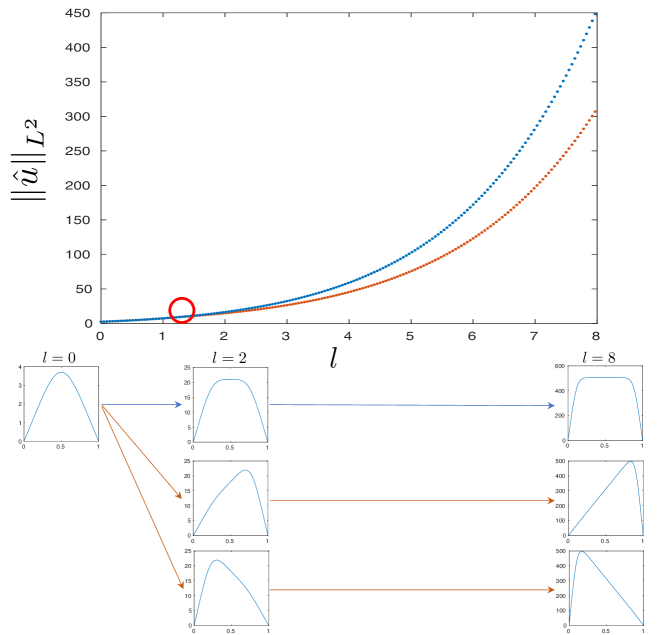
Figure 1: Solution curves for (1) on the unit line segment $(0,1)$.

5.2 Numerical results on the unit square

We apply our method to $\Omega=(0,1)^{2}$ in this subsection. As in Subsection 5.1, we again restrict solution spaces and their finite-dimensional subspaces to look for symmetric solutions. The following sub-solution spaces of $H^{1}_{0}(\Omega)$ are endowed with the same topology:

$$V^{1} :=\left\{u\in H^{1}_{0}(\Omega):u\text{ is symmetric with respect to }x=\frac{1}{2}\right\},$$

$$V^{2} :=\left\{u\in H^{1}_{0}(\Omega):u\text{ is symmetric with respect to }y=x\right\},$$

$$V^{3} :=\left\{u\in H^{1}_{0}(\Omega):u\text{ is symmetric with respect to }y=x\text{ and }y=-x+1\right\},$$

$$V^{4} :=\left\{u\in H^{1}_{0}(\Omega):u\text{ is symmetric with respect to }x=\frac{1}{2},y=\frac{1}{2},y=x\text{, and }y=-x+1\right\}.$$

Then, using $\phi_{i}$ defined in (24), we construct finite-dimensional subspaces $V^{i}_{M}~{}(M\geq 2)$ for each $V^{i}$ ($i=1,2,3,4$) as

$$V^{1}_{M} :=\left\{\sum_{i=1\atop\text{$i$ is odd}}^{M}~{}\sum_{j=1}^{M}~{}u_{i,j}\phi_{i}(x)\phi_{j}(y)~{}:~{}u_{i,j}\in\mathbb{R}\right\},$$

$$V^{2}_{M} :=\left\{~{}\sum_{i=1}^{M}~{}~{}\sum_{j=i}^{M}~{}u_{i,j}\psi_{i,j}(x,y)~{}:~{}u_{i,j}\in\mathbb{R}\right\},$$

$$V^{3}_{M} :=\left\{\sum_{i=1\atop\text{$i$ is odd}}^{M}\sum_{j=i\atop\text{$j$ is odd}}^{M}u_{i,j}\psi_{i,j}(x,y)+\sum_{i=2\atop\text{$i$ is even}}^{M}\sum_{j=i\atop\text{$j$ is even}}^{M}u_{i,j}\psi_{i,j}(x,y)~{}:~{}u_{i,j}\in\mathbb{R}\right\},$$

$$V^{4}_{M} :=\left\{\sum_{i=1\atop\text{$i$ is odd}}^{M}\sum_{j=i\atop\text{$j$ is odd}}^{M}u_{i,j}\psi_{i,j}(x,y)~{}:~{}u_{i,j}\in\mathbb{R}\right\},$$

where $\psi_{i,j}$ is defined as

$$\psi_{i,j}(x,y):=\phi_{i}(x)\phi_{j}(y)+\phi_{j}(x)\phi_{i}(y),~{}~{}(x,y)\in\Omega,$$

which is symmetric with respect to the line $y=x$. Note that we use the same notation $V^{1}$ and $V^{1}_{M}$ with different meanings than in Subsection 5.1. The method presented in Sections 3 and 4 can be directly applied when the function spaces $H^{1}_{0}(\Omega)$ and $V_{M}$ are replaced with $V^{i}$ and $V^{i}_{M}$, respectively. In the solution space $V^{i}_{M}$, approximate solutions $\hat{u}$ were obtained by solving the matrix equation

$${\rm Find} ~{}\hat{u}\in V^{i}_{M}~{}{\rm s.t.}~{}\left(\nabla\hat{u},\nabla v_{M}\right)_{L^{2}}=\left(f(\hat{u}),v_{M}\right)_{L^{2}}~{}~{}{\rm for~{}all}~{}v_{M}\in V^{i}_{M}$$ (27)

via the usual Newton method. Restricting solution spaces reduces the amount of calculation for the same reasons as described in Subsection 5.1. Using the evaluation (23) when $\Omega=(0,1)^{2}$ with the center $\boldsymbol{x_{0}}=(1/2,1/2)$, we evaluated the Lipschitz constant $L$ as

$$L\leq 6\left(\frac{1}{\sqrt{2}}\right)^{l}C^{3}_{4}(\|\hat{u}\|_{L^{4}}+C_{4}r).$$

Tables 2 and 3 show the approximate solutions together with their verification results. The red dashed lines indicate the symmetry of each solution. We again set $\tau\approx 4.9407\times 10^{-324}$, the minimal positive floating-point number after zero. In the tables, $\|F(\hat{u})\|_{H^{-1}}$, $\|F^{\prime-1}_{\hat{u}}\|_{\mathcal{L}(H^{-1},H^{1}_{0})}$, $L$, $\alpha$, and $\beta$ denote the constants required by Theorem 3. Moreover, $r_{A}$ and $r_{R}$ denote an upper bound for absolute error $\|u-\hat{u}\|_{H^{1}_{0}}$ and relative error $\|u-\hat{u}\|_{H^{1}_{0}}/\|\hat{u}\|_{H^{1}_{0}}$, respectively. The values in row “Peak” represent upper bounds for the maximum values of the corresponding approximate solutions. We see that error bounds are affected by the number of peaks — fewer peaks lead to larger error bounds. As $l$ increases, the peaks approach the corners of the domain and become higher. Therefore, a larger $l$ makes verification based on Theorem 3 more difficult. We succeeded in proving the existence of solutions in all cases in which $l=0,2,4$, including three-peak solutions not found in [6].

The values in rows $\mu_{1}$–$\mu_{5}$ represent approximations of the five smallest eigenvalues of (16) discretized in $V_{30}\subset H^{1}_{0}(\Omega)$, which is spanned by the basis functions $\phi_{n}$ ($n=1,2,\cdots,30$) without the restriction of symmetry. When $l=4$, the number of negative eigenvalues $\mu$ coincides with the number of peaks.

Our approximate computation obtained Figure 2, the solution curves of (1) for $0\leq l\leq 8$ ($l$ is always a multiple of 0.05). If the vertical axis scaling is changed, the curves coincide with those in [6, Figure 2] except for that corresponding to the three-peak solutions after the point around $[2.35,2.40]$. The verified points where $l=0,2,4$ lie on the solution curves. According to Figure 2, two bifurcation points are expected to exist around $[0.55,0.60]$ and $[2.35,2.40]$. We expect the single-solution curve bifurcates to three at the first bifurcation point around $[0.55,0.60]$, and then one of them further bifurcates to three at the second point around $[2.35,2.40]$.

Table 2: Verification results for $l=0,2$ on the unit square $(0,1)^{2}$.

$l$	0	2
3D $\hat{u}$
2D $\hat{u}$
Solution space	$V^{4}$	$V^{4}$	$V^{1}$	$V^{2}$
$M_{u}$	40	40	60	60
$M$	40	40	40	40
$\|F(\hat{u})\|_{H^{-1}}$	1.17370e-7	3.96407e-7	1.19312e-8	4.22257e-7
$\|F^{\prime-1}_{\hat{u}}\|_{\mathcal{L}(H^{-1},H^{1}_{0})}$	1.70326	2.26200	15.19763	36.47472
$L$	6.78398e-1	1.64252	1.43209	1.21150
$\alpha$	1.99910e-7	8.96672e-7	1.81325e-7	1.54017e-5
$\beta$	1.15549	3.71537	21.76424	44.18887
$r_{A}$	4.63296e-8	2.55597e-7	1.44557e-7	2.48634e-5
$r_{R}$	3.76958e-9	3.98528e-9	2.45351e-9	4.63166e-7
Peak	6.62326	24.36528	29.03437	29.20268
$\mu_{1}$	-1.99999	-1.99999	-1.99999	-1.99999
$\mu_{2}$	0.220034	-0.410090	-0.273589	0.196622
$\mu_{3}$	0.220034	-0.410090	0.233061	0.208937
$\mu_{4}$	0.604521	0.114826	0.457439	0.585268
$\mu_{5}$	0.658421	0.298974	0.517021	0.639470

Solution space: restricted solution space $V^{i}\subset H^{1}_{0}(\Omega)$
$M_{u}$: number of basis functions with respect to $x$ and $y$ for constructing approximate solution $\hat{u}\in V^{i}_{M_{u}}$
$M$: number of basis functions with respect to $x$ and $y$ for calculating $\lambda^{M}$
$\|F(\hat{u})\|_{H^{-1}}$: upper bound for the residual norm estimated via (13)
$\|F^{\prime-1}_{\hat{u}}\|_{\mathcal{L}(H^{-1},H^{1}_{0})}$: upper bound for the inverse operator norm estimated via Theorem 4
$L$: upper bound for Lipschitz constant satisfying (12)
$\alpha$: upper bound for $\alpha$ required in Theorem 3
$\beta$: upper bound for $\beta$ required in Theorem 3
$r_{A}$: upper bound for absolute error $\|u-\hat{u}\|_{H^{1}_{0}}$
$r_{R}$: upper bound for relative error $\|u-\hat{u}\|_{H^{1}_{0}}/\|\hat{u}\|_{H^{1}_{0}}$
Peak: upper bound for the maximum values of the corresponding approximation
$\mu_{1}$–$\mu_{5}$: approximations of the five smallest eigenvalues of (16)

Table 3: Verification results for $l=4$ on the unit square $(0,1)^{2}$.

$l$	4
3D $\hat{u}$
2D $\hat{u}$
Solution space	$V^{4}$	$V^{3}$	$V^{1}$	$V^{2}$	$V^{2}$
$M_{u}$	70	70	70	70	70
$M$	80	80	80	80	80
$\|F(\hat{u})\|_{H^{-1}}$	1.88534e-11	7.91070e-6	4.76970e-7	8.47044e-6	3.47384e-8
$\|F^{\prime-1}_{\hat{u}}\|_{\mathcal{L}(H^{-1},H^{1}_{0})}$	6.82420	24.18779	78.96665	21.26750	47.44875
$L$	2.31308	1.46531	1.55126	1.18832	1.97091
$\alpha$	1.28659e-10	1.91343e-4	3.76648e-5	1.80145e-4	1.64830e-6
$\beta$	15.78486	35.44250	1.22498e+2	25.27251	93.51720
$r_{A}$	4.95952e-11	1.73351e-4	8.76586e-5	1.53306e-4	2.32064e-6
$r_{R}$	2.35369e-13	9.86681e-7	5.12219e-7	1.20925e-6	1.16657e-8
Peak	62.30489	68.15045	66.28947	69.69524	64.16408
$\mu_{1}$	-1.99999	-1.99996	-1.99999	-1.99999	-1.99999
$\mu_{2}$	-0.995156	-1.86714	-1.64594	0.177691	-1.46267
$\mu_{3}$	-0.995156	0.166245	0.130875	0.251043	-1.14006
$\mu_{4}$	-0.689431	0.205039	0.253364	0.591950	0.131828
$\mu_{5}$	0.210478	0.258004	0.272595	0.658008	0.175494

Solution space: restricted solution space $V^{i}\subset H^{1}_{0}(\Omega)$
$M_{u}$: number of basis functions with respect to $x$ and $y$ for constructing approximate solution $\hat{u}\in V^{i}_{M_{u}}$
$M$: number of basis functions with respect to $x$ and $y$ for calculating $\lambda^{M}$
$\|F(\hat{u})\|_{H^{-1}}$: upper bound for the residual norm estimated via (13)
$\|F^{\prime-1}_{\hat{u}}\|_{\mathcal{L}(H^{-1},H^{1}_{0})}$: upper bound for the inverse operator norm estimated via Theorem 4
$L$: upper bound for Lipschitz constant satisfying (12)
$\alpha$: upper bound for $\alpha$ required in Theorem 3
$\beta$: upper bound for $\beta$ required in Theorem 3
$r_{A}$: upper bound for absolute error $\|u-\hat{u}\|_{H^{1}_{0}}$
$r_{R}$: upper bound for relative error $\|u-\hat{u}\|_{H^{1}_{0}}/\|\hat{u}\|_{H^{1}_{0}}$
Peak: upper bound for the maximum values of the corresponding approximation
$\mu_{1}$–$\mu_{5}$: approximations of the five smallest eigenvalues of (16)

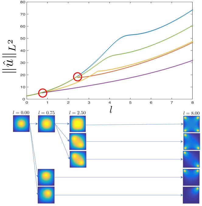
Figure 2: Solution curves for (1) on the unit square $(0,1)^{2}$.

6 Conclusion

We designed a numerical verification method for proving the existence of solutions of the Hénon equation (1) on a bounded domain based on the Newton-Kantorovich theorem. We applied our method to the domains $\Omega=(0,1)^{N}$ $(N=1,2)$, proving the existence of several solutions of (1) nearby a numerically computed approximation $\hat{u}$. In particular, we found a set of undiscovered solutions with three peaks on the square domain $\Omega=(0,1)^{2}$. Approximate computations generated the solution curves of (1) for $0\leq l\leq 8$ in Figures 1 and 2. Future work should verify the existence of solutions for arbitrary $l\in[0,a]$, given a large $a>0$, and prove the bifurcation structure for (1) in a strict mathematical sense.

7 Acknowledgements

We thank Dr. Kouta Sekine (Toyo University, Japan) for his helpful advice. We also express our gratitude to anonymous referees for insightful comments. This work was supported by CREST, JST Grant Number JPMJCR14D4; and by JSPS KAKENHI Grant Number JP19K14601.

References

• [1] M. Hénon, Numerical experiments on the stability of spherical stellar systems, Astronomy and astrophysics 24 (1973) 229–238.
• [2] B. Gidas, W.-M. Ni, L. Nirenberg, Symmetry and related properties via the maximum principle, Communications in Mathematical Physics 68 (3) (1979) 209–243.
• [3] B. Breuer, M. Plum, P. McKenna, Inclusions and existence proofs for solutions of a nonlinear boundary value problem by spectral numerical methods, in: Topics in Numerical Analysis, Springer 15, (2001) 61–77.
• [4] D. Smets, M. Willem, J. Su, Non-radial ground states for the Hénon equation, Communications in Contemporary Mathematics 4 (03) (2002) 467–480.
• [5] A. L. Amadori, F. Gladiali, Bifurcation and symmetry breaking for the Hénon equation, Advances in Differential Equations 19 (7/8) (2014) 755–782.
• [6] Z. Yang, Z. Li, H. Zhu, Bifurcation method for solving multiple positive solutions to Henon equation, Science in China Series A: Mathematics 51 (12) (2008) 2330–2342.
• [7] Z. Li, Z. Yang, H. Zhu, Bifurcation method for computing the multiple positive solutions to p-Henon equation, Applied Mathematics and Computation 220 (2013) 593–601.
• [8] Z. Li, Z. Yang, H. Zhu, A bifurcation method for solving multiple positive solutions to the boundary value problem of the Henon equation on a unit disk, Computers & Mathematics with Applications 62 (10) (2011) 3775–3784.
• [9] Z. Li, H. Zhu, Z. Yang, Bifurcation method for solving multiple positive solutions to Henon equation on the unit cube, Communications in Nonlinear Science and Numerical Simulation 16 (9) (2011) 3673–3683.
• [10] M. T. Nakao, M. Plum, Y. Watanabe, Numerical Verification Methods and Computer-Assisted Proofs for Partial Differential Equations, Springer, (2019).
• [11] K. Tanaka, K. Sekine, M. Mizuguchi, S. Oishi, Sharp numerical inclusion of the best constant for embedding $H_{0}^{1}(\Omega)\hookrightarrow L^{p}(\Omega)$ on bounded convex domain, Journal of Computational and Applied Mathematics 311 (2017) 306–313.
• [12] P. Deuflhard, G. Heindl, Affine invariant convergence theorems for Newton’s method and extensions to related methods, SIAM Journal on Numerical Analysis 16 (1) (1979) 1–10.
• [13] M. Plum, Computer-assisted proofs for semilinear elliptic boundary value problems, Japan journal of industrial and applied mathematics 26 (2-3) (2009) 419–442.
• [14] H. Behnke, The calculation of guaranteed bounds for eigenvalues using complementary variational principles, Computing 47 (1) (1991) 11–27.
• [15] S. M. Rump, Intlab–interval laboratory, in: Developments in reliable computing, Springer, (1999) 77–104.
URL http://www.ti3.tuhh.de/rump/
• [16] S. Miyajima, Numerical enclosure for each eigenvalue in generalized eigenvalue problem, Journal of Computational and Applied Mathematics 236 (9) (2012) 2545–2552.
• [17] P. Grisvard, Elliptic problems in nonsmooth domains, SIAM, (2011).
• [18] K. Tanaka, A. Takayasu, X. Liu, S. Oishi, Verified norm estimation for the inverse of linear elliptic operators using eigenvalue evaluation, Japan Journal of Industrial and Applied Mathematics 31 (3) (2014) 665–679.
• [19] X. Liu, A framework of verified eigenvalue bounds for self-adjoint differential operators, Applied Mathematics and Computation 267 (2015) 341–355.
• [20] K. Tanaka, K. Sekine, S. Oishi, Numerical verification method for positivity of solutions to elliptic equations , RIMS Kôkyûroku 2037 (2011) 125–140.
• [21] S. Kimura, N. Yamamoto, On explicit bounds in the error for the $H^{1}_{0}$-projection into piecewise polynomial spaces, Bulletin informatics and cybernetics 31 (2) (1999) 109-115.
• [22] M. Kashiwagi, kv library, (2020).
URL http://verifiedby.me/kv/