Schrödinger operators with a switching effect

Abstract

This paper summarizes the contents of a plenary talk given at the 14th Biennial Conference of Indian SIAM in Amritsar in February 2018. We discuss here the effect of an abrupt spectral change for some classes of Schrödinger operators depending on the value of the coupling constant, from below bounded and partly or fully discrete, to the continuous one covering the whole real axis. A prototype of such a behavior can be found in Smilansky-Solomyak model devised to illustrate that an an irreversible behavior is possible even if the heat bath to which the systems is coupled has a finite number of degrees of freedom and analyze several modifications of this model, with regular potentials or a magnetic field, as well as another system in which $x^{p}y^{p}$ potential is amended by a negative radially symmetric term. Finally, we also discuss resonance effects in such models.

1 Introduction

The class of problems we are going to discuss here has a twofold motivation. Let us start with physics. It is well known that while the equations of motion governing quantum dynamics are invariant with respect to time reversal, we often encounter quantum systems behaving in an irreversible way, for instance, spontaneous decays of particles and nuclei, inelastic scattering processes in nuclear, atomic or molecular systems, or the current passing through a microscopic element attached to poles of a battery. Furthermore, an irreversible process par excellence is, of course, the wave packet reduction which is the core of Copenhagen description of a measuring process performed on a quantum system.

The description of such a process is typically associated with enlarging the state Hilbert space, conventionally referred to as coupling the system to a heat bath. It is generally accepted that to obtain an irreversible behavior through such a coupling, the model has to exhibit typical properties, in particular

• the bath is a system with infinite number of degrees of freedom

• the bath Hamiltonian has a continuous spectrum

• the presence (or absence) of irreversible modes is determined by the energies involved rather than the coupling strength

While this all is without any doubt true in many cases, one of our aims here is to show that neither of the above need not be true in general. To make this point, Uzy Smilansky constructed a simple model which will be our starting point here. In a sense he did a similar thing as Agatha Christie: when some people tried to introduce in the 1920s mystery rules saying, in particular, that in any such such book there must be a single murderer, she wrote Murder on the Orient Express in which everyone is a killer, except Hercule Poirot, of course.

On the other hand, as a mathematician one may ask whether a small change of the coupling constant can have a profound influence on the spectrum. Posed like that the answer is trivial: consider the the one-dimensional Schrödinger operator

$$H_{\lambda}=-\frac{\mathrm{d}^{2}}{\mathrm{d}x^{2}}+\lambda x^{2}\,;$$

it is obvious that all $\lambda=\omega^{2}>0$ the spectrum of such an operator is purely discrete, $\sigma(H_{\lambda})=\{(2n+1)\omega:\>n=0,1,\dots\}$, while for $\lambda=0$ and $\lambda<0$ we have $\sigma(H_{\lambda})=[0,\infty)$ and $\sigma(H_{\lambda})=\mathbb{R}$, respectively. A much more subtle question is whether similar things could happen if the potential modification concerns a small part of the configuration space, or even a ‘set of zero measure’. Smilansky model and its various modifications we are going to discuss provide an affirmative answer.

Let us describe briefly the contents of the paper. In the next section we summarize the known results about Smilansky-Solomyak model and present a numerical method to analyze its discrete spectrum. Sec. 3 is devoted to discussion of various modifications of the model consisting, in particular, in replacing the $\delta$ interaction ‘channel’ by a regular potential one or, on the contrary, by the more singular $\delta^{\prime}$ interaction, or adding a homogeneous magnetic field. In Sec. 4 we discuss another model exhibiting a similar behaviour, a two-dimensional Schrödinger operator with the potential consisting of the $x^{p}y^{p}$ part amended by a negative radially symmetric term. In Sec. 5 we return to the original Smilansky-Solomyak model and show that it also has a rich resonance structure. Finally, in conclusion we will mention several open questions.

2 Smilansky-Solomyak model

Let us first describe the model proposed by Uzy Smilansky in Sm04 which in its simplest form describes a one-dimensional system interacting with a caricature heat bath represented by a single harmonic oscillator. Its mathematical properties and various extensions were subsequently analyzed by Michael Solomyak – let us pay a memory to this great mathematician who left us two years ago – and coauthors in ES05I ; ES05II ; NS06 ; RS07 ; S04FAA ; S06 ; S06JPA from the spectral point view, the corresponding time evolution was discussed in G11 ; G18 .

With this history of the problem in mind, it is appropriate to speak of the Smilansky-Solomyak model. At the same time, it is useful to note that while mathematically it is the same thing, physically there may be two ways in which the system is understood. In the original Smilansky treatment one considers two one-dimensional systems coupled mutually, while Solomyak et al. interpreted it in PDE terms as being described by a two-dimensional Schrödinger operator,

$$H_{\mathrm{Sm}}=-\frac{\partial^{2}}{\partial x^{2}}+\frac{1}{2}\left(-\frac{\partial^{2}}{\partial y^{2}}+y^{2}\right)+\lambda y\delta(x),$$ (1)

on $L^{2}(\mathbb{R}^{2})$; it is easy to see that that one may consider $\lambda\geq 0$ only without loss of generality. We will stick here to the latter interpretation because it opens way to a wider class of possible generalizations.

Let us summarize the known results about spectral properties of the operator (1):

• The existence of a spectral transition: if $|\lambda|>\sqrt{2}$ the particle can escape to infinity along the singular ‘channel’ in the $y$ direction. In spectral terms, this corresponds to the switch from a positive spectrum to a below unbounded one at $|\lambda|=\sqrt{2}$. At the heuristic level, the mechanism of this spectral transition is easy to understand: we have an effective variable decoupling far from the $x$-axis and the oscillator potential competes there with the $\delta$ interaction eigenvalue $-\frac{1}{4}\lambda^{2}y^{2}$.

• The eigenvalue absence: for any $\lambda\geq 0$ there are no eigenvalues $\geq\frac{1}{2}$. If $|\lambda|>\sqrt{2}$, the point spectrum of $H_{\mathrm{Sm}}$ is empty.

• The existence of eigenvalues: in the subcritical case, $0<|\lambda|<\sqrt{2}$, we have $H_{\mathrm{Sm}}\geq 0$. The point spectrum is then nonempty and finite, and

  $$N(\textstyle{\frac{1}{2}},H_{\mathrm{Sm}})\sim\frac{1}{4\sqrt{2(\mu(\lambda)-1)}}$$ (2)

  holds as $\lambda\to\sqrt{2}-$, where $\mu(\lambda):=\sqrt{2}/\lambda$.

• The absolute continuity: in the supercritical case, $|\lambda|>\sqrt{2}$, we have $\sigma(H_{\mathrm{Sm}})=\sigma_{\mathrm{ac}}(H_{\mathrm{Sm}})=\mathbb{R}$.

We are not going to give proofs of these claims referring to the papers quoted above, instead we will show how the the discrete spectrum can be found numerically following ELT17a which can provide additional insights. At the time, however, the method we use, rephrasing the task as a spectral problem for Jacobi matrices is the core of the proofs done by Solomyak et al. providing thus a feeling of what is the technique involved.

In the halfplanes $\pm x>0$ the wave functions can be expanded using the ‘transverse’ base spanned by the functions

$$\psi_{n}(y)=\frac{1}{\sqrt{2^{n}n!\sqrt{\pi}}}\>\mathrm{e}^{-y^{2}/2}H_{n}(y)$$ (3)

corresponding to the oscillator eigenvalues $n+\frac{1}{2},\>n=0,1,2,\dots\,$. Furthermore, one can make use of the mirror symmetry w.r.t. $x=0$ and divide $H_{\lambda}$ into the trivial odd part $H_{\lambda}^{(-)}$ and the even part $H_{\lambda}^{(+)}$ which is equivalent to the operator on the halfplane, $L^{2}(\mathbb{R}\times(0,\infty))$, with the same symbol determined by the boundary condition

$$f_{x}(0+,y)=\frac{1}{2}\,\alpha yf(0+,y).$$ (4)

We substitute the Ansatz

$$f(x,y)=\sum_{n=0}^{\infty}c_{n}\,\mathrm{e}^{-\kappa_{n}x}\psi_{n}(y)$$ (5)

with $\kappa_{n}:=\sqrt{n+\frac{1}{2}-\epsilon}$ into (4); this yields for the sought solution with the energy $\epsilon$ the equation

$$B_{\lambda}c=0,$$ (6)

where $c$ is the coefficient vector and $B_{\lambda}$ is the operator in $\ell^{2}$ with the representation

$$(B_{\lambda})_{m,n}=\kappa_{n}\delta_{m,n}+\frac{1}{2}\lambda(\psi_{m},y\psi_{n}).$$ (7)

It is obvious that the matrix is in fact tridiagonal because

$$(\psi_{m},y\psi_{n})=\frac{1}{\sqrt{2}}\big{(}\sqrt{n+1}\,\delta_{m,n+1}+\sqrt{n}\,\delta_{m,n-1}\big{)}.$$ (8)

To solve the equation (6) numerically one truncates the matrix (7). The size depends on $\lambda$, the most difficult is the weakly bound state corresponding to small $\lambda$ where the truncation size should be of order of $10^{4}$ to achieve a numerically stable solution.

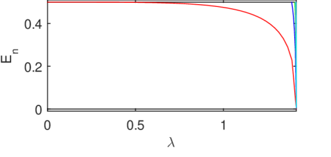
Figure 1: Discrete spectrum of $H_{\mathrm{Sm}}$ as a function of the coupling constant $\lambda$

The result is plotted in Fig. 1. In coincidence with the theoretical result quoted above the discrete spectrum is nonempty for nonzero $\lambda$. It may seem that it consists of a single eigenvalues but a closer look shows that the second one appears at $\lambda\approx 1.387559$; the next thresholds are $1.405798,1.410138,1.41181626,1.41263669,\dots\>$.

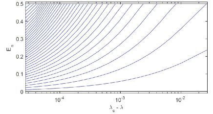
Figure 2: Discrete spectrum of $H_{\mathrm{Sm}}$ near the critical value of the coupling constant

To have a better insight one can plot the discrete spectrum near the critical coupling in the semilogarithmic scale as shown in Fig. 2. We see that in this regime many eigenvalues appear which gradually fill the interval $(0,\frac{1}{2})$ as the critical value $\lambda=\sqrt{2}$ is approached. Fig. 3 shows a comparison of their number indicated by dots with the asymptotics (2); we see a perfect fit.

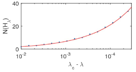
Figure 3: Number of eigenvalues of $H_{\mathrm{Sm}}$ vs. the asymptotics (2)

The numerical solution also indicates other properties. For instance, plotting in Fig. 4 the eigenvalue curve for small values of $\lambda$ in the logarithmic scale we see that it behaves as $E_{1}(\lambda)=\frac{1}{2}-c\lambda^{4}+o(\lambda^{4})$ as $\lambda\to 0$, with $c\approx 0.0156$.

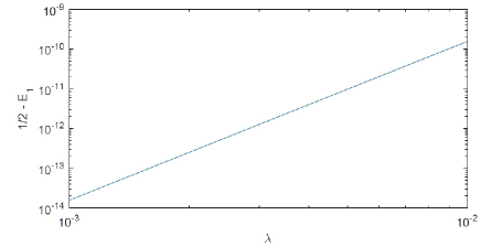
Figure 4: Weak coupling asymptotics of $H_{\mathrm{Sm}}$

In fact, the coefficient value can be found exactly to be $c=0.015625$. To this aim, we write the equation (6) explicitly in components as

$$\sqrt{\mu_{\lambda}}c^{\lambda}_{0}+\frac{\lambda}{2\sqrt{2}}c^{\lambda}_{1}=0,$$

$$\frac{\sqrt{k}\lambda}{2\sqrt{2}}c^{\lambda}_{k-1}+\sqrt{k+\mu_{\lambda}}c^{\lambda}_{k}+\frac{\sqrt{k+1}\lambda}{2\sqrt{2}}c^{\lambda}_{k+1}=0, \;\;k\geq 1\,,$$

where $\mu_{\lambda}:=\frac{1}{2}-E_{1}(\lambda)$ and $c^{\lambda}=\{c^{\lambda}_{0},c^{\lambda}_{1},\dots\}$ is the corresponding normalized eigenvector of $B_{\lambda}$. Using the above relations and simple estimates, we get from here

$$\sum_{k=1}^{\infty}|c_{k}^{\lambda}|^{2}\leq\frac{3}{4}\lambda^{2}\quad\text{and}\quad c_{0}^{\lambda}=1+\mathcal{O}(\lambda^{2})$$ (10)

as $\lambda\to 0+$, hence we have in particular $c_{1}^{\lambda}=\frac{\lambda}{2\sqrt{2}}+\mathcal{O}(\lambda^{2})$. The first of the above relations then gives $\mu_{\lambda}=\frac{\lambda^{4}}{64}+\mathcal{O}(\lambda^{5})$ as $\lambda\to 0+$, in other words

$$E_{1}(\lambda)=\frac{1}{2}-\frac{\lambda^{4}}{64}+\mathcal{O}(\lambda^{5}),$$ (11)

however, the mentioned coefficient $0.015625$ is nothing else than $\frac{1}{64}$. Furthermore with the knowledge of the solution to (6) we can return to (5) and compute the eigenfunctions.

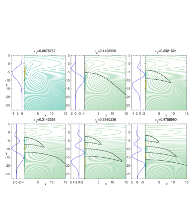
Figure 5: The eigenfunctions of $H_{\mathrm{Sm}}$ for $\lambda=1.4128241$

In Fig. 5 we plot them for a value close to the critical one, namely $\lambda=\sqrt{2}-0.0086105$. As expected, they are stretched along the axis of the oscillator ‘channel’ and the part of the $y$-axis where the singular interaction is attractive; the he curves at the left side show the $y$-cuts of the eigenfunctions. The ground state has no zeros and the number of the nodal lines of the $n$th eigenfunction, $n=1,2,\dots\>$, is $[\frac{1}{2}n]$, thus only the first excited state is Courant sharp.

3 Variations on the model

We have mentioned in the introduction that various extensions of the Smilansky-Solomyak model described above had been worked out, for instance, using a ‘heat bath’ consisting of more than one oscillator, replacing the line by a loop or a graph, etc. We will not discuss them, instead we will analyze several other modifications.

3.1 Regular version of the model

The first one is motivated by the question whether one can observe a similar effect for Schrödinger operators with the $\delta$ interaction replaced by a regular potentials. It was asked by Italo Guarneri in G11 with a clear motivation: he employed (a modification of) the system described above as a model of the measuring process in quantum mechanics in which the supercritical behaviour is interpreted as a wave packet reduction. This naturally inspires the question how the corresponding classical dynamics would look like, and this in turn requires a setting in which the problem can be analyzed in terms of classical mechanics; the first step in this direction has been made in the recent paper G18 .

We observe first that the coupling cannot be now linear in $y$ and the profile of the channel has to change with the variable $y$. We replace the $\delta$ by a family of shrinking potentials the mean of which matches the $\delta$ coupling constant, $\int U(x,y)\,\mathrm{d}x\sim y$. This can be achieved, e.g., by choosing $U(x,y)=\lambda y^{2}V(xy)$ for a fixed function $V$. This motivates us to investigate the following operator on $L^{2}(\mathbb{R}^{2})$,

$$H=-\frac{\partial^{2}}{\partial x^{2}}-\frac{\partial^{2}}{\partial y^{2}}+\omega^{2}y^{2}-\lambda y^{2}V(xy),$$ (12)

where $\omega,\,a$ are positive constants and the potential $V$ is a nonnegative function with bounded first derivative and $\mathrm{supp}\,V\subset[-a,a]$. By Faris-Lavine theorem $H$ is e.s.a. on $C_{0}^{\infty}(\mathbb{R}^{2})\,$ – cf. (RS, , Thms. X.28 and X.38) – and the same argument can be applied to various generalizations of the operator (12), with more than one ‘decay’ channel, periodicity in the variable $x$, etc.

To state the result we need a one-dimensional comparison operator $L=L_{V}$, namely

$$L=-\frac{\mathrm{d}^{2}}{\mathrm{d}x^{2}}+\omega^{2}-\lambda V(x)$$ (13)

on $L^{2}(\mathbb{R})$ with the domain $H^{2}(\mathbb{R})$. What matters is the sign of its spectral threshold; since $V\geq 0$, the latter is a monotonous function of $\lambda$ and there is a $\lambda_{\mathrm{crit}}>0$ at which the sign changes. First of all, we have the following result BE14 .

Theorem 3.1

Under the stated assumption, the spectrum of the spectrun of $H$ is bounded from below provided the operator $L$ is positive.

Sketch of the proof. The claim can proved using Neumann bracketing, imposing additional boundary conditions at the lines $y=\pm\ln n$, $n=2,3,\dots$, and showing that the components of $H$ in these strips have a uniform lower bound by an operator unitarily equivalent to $L$, cf. BE14 for details. ∎

One the other hand, in the supercritical case when the transverse channel principal eigenvalue dominates over the harmonic oscillator contribution, the spectral behavior changes BE14 .

Theorem 3.2

Under our hypotheses, $\sigma(H)=\mathbb{R}$ holds if $\inf\sigma(L)<0$.

Sketch of the proof. The argument relies on a choice of an appropriate Weyl sequence: we have to find $\{\psi_{k}\}_{k=1}^{\infty}\subset D(H)$ such that $\|\psi_{k}\|=1$ which contains no convergent subsequence, and at same time

$$\|H\psi_{k}-\mu\psi_{k}\|\to 0\quad\text{as}\quad k\to\infty.$$ (14)

Specifically, we choose

$$\psi_{k}(x,y)=h(xy)\,\mathrm{e}^{i\epsilon_{\mu}(y)}\chi_{k}\left(\frac{y}{n_{k}}\right)+\frac{f(xy)}{y^{2}}\,\mathrm{e}^{i\epsilon_{\mu}(y)}\chi_{k}\left(\frac{y}{n_{k}}\right),$$

where $\epsilon_{\mu}(y):=\int_{\sqrt{|\mu|}}^{y}\sqrt{t^{2}+\mu}\,\mathrm{d}t$, $\>h$ is the normalized ground-state eigenfunction of $L$, furthermore $\,f(t):=-\frac{i}{2}\,t^{2}h(t)$, and finally, $\chi_{k}$ are suitable, compactly supported mollifier functions, cf. BE14 for details. ∎

The regular version shares also other properties with the original Smilansky-Solomyak model, namely BE17a :

• in the subcritical case, $\inf\sigma(L)>0$, we have $\sigma_{\mathrm{ess}}(H)=[\omega,\infty)$ and a nonempty $\sigma_{\mathrm{disc}}(H)\subset[0,\omega)$

• in the critical case, $\inf\sigma(L)=0$, we have $\sigma(H)=\sigma_{\mathrm{ess}}(H)=[0,\infty)$

3.2 Magnetic version of the model

One can also consider another modification of Smilansky-Solomyak model in which the system is placed into a homogeneous magnetic field perpendicular to the plane representing the configuration space, described thus by the Hamiltonian

$$H=(i\nabla+A)^{2}+\omega^{2}y^{2}+\lambda y\delta(x),$$ (15)

where $A$ is a suitable vector potential; note that in this case the original Smilansky interpretation is lost. The spectral properties are similar, in the subcritical case we now have $\sigma_{\mathrm{ess}}(H(A))=[\sqrt{B^{2}+\omega^{2}},\infty)$ but again a sufficiently small nonzero $\lambda$ gives rise to a discrete spectrum which fills the interval $[0,\sqrt{B^{2}+\omega^{2}})$ as $|\lambda|$ approaches the critical coupling $2\omega$, and above this value the spectrum fills the whole real line. The effect of the magnetic field on the regular version of the model is similar, cf. BE17b for details.

3.3 The $\delta^{\prime}$ version of the model

One can also say that the spectral transition effect is robust. To illustrate this claim let us consider the version of the model in which the interaction is replaced by a more singular one, specifically the one known as $\delta^{\prime}\>$ AGHH . The Hamiltonian then corresponds to the differential expression

$$H_{\beta}\psi(x,y)=-\frac{\partial^{2}\psi}{\partial x^{2}}(x,y)+\frac{1}{2}\left(-\frac{\partial^{2}\psi}{\partial y^{2}}(x,y)+y^{2}\psi(x,y)\right)$$ (16)

with the domain consisting of $\psi\in H^{2}((0,\infty)\times\mathbb{R})\oplus H^{2}((-\infty,0)\times\mathbb{R})$ such that

$$\psi(0+,y)-\psi(0-,y)=\frac{\beta}{y}\frac{\partial\psi}{\partial x}(0+,y)\,,\quad\frac{\partial\psi}{\partial x}(0+,y)=\frac{\partial\psi}{\partial x}(0-,y).$$ (17)

The problem can be treated by a modification of the methods employed in ES05I ; ES05II ; NS06 ; RS07 ; S04FAA ; S06 ; S06JPA leading to the following results which we present referring to EL18 for the proofs. Let $\mathfrak{m}_{\mathrm{ac}}$ be the multiplicity of the absolutely continuous spectrum.

Theorem 3.3

The spectrum of operator $H_{0}$ is purely ac, $\sigma(H_{0})=[\frac{1}{2},\infty)$ with the multiplicity $\mathfrak{m}_{\mathrm{ac}}(E,H_{0})=2n$ for $E\in(n-\frac{1}{2},n+\frac{1}{2})$, $\,n\in\mathbb{N}$. For $\beta>2\sqrt{2}$ the ac spectrum of $H_{\beta}$ coincides with $\sigma(H_{0})$. For $\beta\leq 2\sqrt{2}$ there is a new branch of continuous spectrum added to the spectrum; for $\beta=2\sqrt{2}$ we have $\sigma(H_{\beta})=[0,\infty)$ and for $\beta<2\sqrt{2}$ the spectrum covers the whole real line.

We note in passing that with the standard convention used here, small values of the parameter $\beta$ represent a strong coupling.

Theorem 3.4

Assume $\beta\in(2\sqrt{2},\infty)$, then the discrete spectrum of $H_{\beta}$ is nonempty and lies in the interval $(0,\frac{1}{2})$. The number of eigenvalues is approximately given by

$$\frac{1}{4\sqrt{2\left(\frac{\beta}{2\sqrt{2}}-1\right)}}\quad\mathrm{as}\quad\beta\to 2\sqrt{2}+$$

Theorem 3.5

For large enough $\beta$ there is a single eigenvalue which asymptotically behaves as

$$E_{1}(\beta)=\frac{1}{2}-\frac{4}{\beta^{4}}+\mathcal{O}\left(\beta^{-5}\right).$$

4 Another model

The Smilansky-Solomyak model is not the only system in which the effect of an abrupt spectral transition can be observed. Now we are going to describe another model in which the transition is even more dramatic as a switch from a purely discrete spectrum in the subcritical case to the whole real line in the supercritical one. To begin, recall that there are situations where Weyl’s law fails and the spectrum is discrete even if the classically allowed phase-space volume is infinite. A classical example of such a situation is due to S83 a two-dimensional Schrödinger operator with the potential $V(x,y)=x^{2}y^{2}$, or more generally, $V(x,y)=|xy|^{p}$ with $p\geq 1$. Similar behavior one can also observe for Dirichlet Laplacians in regions with hyperbolic cusps – see GW11 for more recent results and a survey; recall also that using the dimensional-reduction technique of Laptev and Weidl LW00 one can prove tight spectral estimates for such operators.

A common feature of these models is that the particle motion is confined into channels narrowing towards infinity; the increasing ‘steepness’ of those ‘walleyes’ is responsible for the discreteness of the spectrum. This may remain true even for Schrödinger operators whose potential are unbounded from below in which a classical particle can escape to infinity with an increasing velocity. The situation changes, however, if the attraction is strong enough; recall that a similar behavior was noted already in Zn98 . As an illustration, let us thus analyze the following class of operators on $L^{2}(\mathbb{R}^{2})$,

$$L_{p}(\lambda)\,:\;L_{p}(\lambda)\psi=-\Delta\psi+\left(|xy|^{p}-\lambda(x^{2}+y^{2})^{p/(p+2)}\right)\psi,\quad p\geq 1,$$ (18)

where $(x,y)$ are the standard Cartesian coordinates in $\mathbb{R}^{2}$ and the parameter $\lambda$ in the second term of the potential is non-negative; unless its value is important we write it simply as $L_{p}$. Note that $\frac{2p}{p+2}<2$ so the operator is e.s.a. on $C_{0}^{\infty}(\mathbb{R}^{2})$ by Faris-Lavine theorem mentioned above; the symbol $L_{p}$ or $L_{p}(\lambda)$ will always mean its closure. Needless to say, the power in the last term is chosen in a way that makes it possible to play with the balance between the repulsion coming from the narrowing channels and attraction coming from the negative potential part.

Let us start with the subcritical case which occurs for sufficiently small values of $\lambda$. To characterize the smallness quantitatively we need an auxiliary operator which will be an (an)harmonic oscillator Hamiltonian on line,

$$\tilde{H}_{p}\,:\>\tilde{H}_{p}u=-u^{\prime\prime}+|t|^{p}u$$ (19)

on $L^{2}(\mathbb{R})$ with the standard domain. The principal eigenvalue $\gamma_{p}=\inf\sigma(H_{p})$ equals one for $p=2$; for $p\to\infty$ it becomes $\gamma_{\infty}=\frac{1}{4}\pi^{2}$; it smoothly interpolates between the two values; a numerical solution gives true minimum $\gamma_{p}\approx 0.998995$ attained at $p\approx 1.788$; in the semilogarithmic scale the plot of $\gamma_{p}$ looks as shown in Fig. 6

Figure 6: $\gamma_{p}$ as a function of $p$ in the semilogarithmic scale

As we have said, the spectrum is bounded from below and discrete if $\lambda=0$; our first claim EB12 is that this remains to be the case provided $\lambda$ is small enough.

Theorem 4.1

For any $\lambda\in[0,\lambda_{\mathrm{crit}}]$, where $\lambda_{\mathrm{crit}}:=\gamma_{p}$, the operator $L_{p}(\lambda)$ is bounded from below for any $p\geq 1$; if $\lambda<\gamma_{p}$ its spectrum is purely discrete.

Sketch of the proof. Let $\lambda<\gamma_{p}$. By the minimax principle (RS, , Sec. XIII.1) we need to estimate $L_{p}$ from below by a s-a operator with a purely discrete spectrum. To construct it we employ bracketing imposing additional Neumann conditions at concentric circles of radii $n=1,2,\dots\,$. In the estimating operators the variables decouple asymptotically and the spectral behaviour is determined by their angular parts ; to prove the discreteness one has to check that the lowest ev’s in the annuli tend to infinity as $n\to\infty$. For $\lambda=\gamma_{p}$ this is no longer true but the sequence remains bounded from below. ∎

A similar argument can be used in the supercritical case with a few differences:

• now we seek an upper bound to $L_{p}(\lambda)$ by a below unbounded operator, hence we impose Dirichlet conditions on concentric circles,

• the estimating operators have now nonzero contributions from the radial part, however, those are bounded by $\pi^{2}$ independently of $n$,

• the negative $\lambda$-dependent term now outweights the anharmonic oscillator part so that for the annuli operators $L^{\mathrm{D}}_{n,p}$ we have $\inf\sigma(L^{\mathrm{D}}_{n,p})\to-\infty$ as $n\to\infty$.

This yields the following conclusion EB12 :

Proposition 1

The spectrum of $L_{p}(\lambda),\>p\geq 1\,$, is unbounded below from if $\lambda>\lambda_{\mathrm{crit}}$.

One can prove a stronger result, however, using a suitable Weyl sequences constructed in a way similar to that employed in the proof of Theorem 3.1 it is possible to make the following conclusion BEKT16 :

Theorem 4.2

$\sigma(L_{p}(\lambda))=\mathbb{R}$ holds for any $\lambda>\gamma_{p}$ and $p>1$.

In the subcritical case one can derive various results concerning properties of the discrete spectrum. Let us first mention an inequality obtain in a variational way for the proof of which we refer to EB12 . We define $\alpha:=\frac{1}{2}\left(1+\sqrt{5}\right)^{2}\approx 5.236>\gamma_{p}^{-1}$ and denote by $\{\lambda_{j,p}\}_{j=1}^{\infty}$ the eigenvalues of $L_{p}(\lambda)$ arranged in the ascending order, then we can make the following claim:

Proposition 2

To any nonnegative $\lambda<\alpha^{-1}\approx 0.19$ there exists a positive constant $C_{p}$ depending on $p$ only such that the following estimate is valid,

$$\sum_{j=1}^{N}\lambda_{j,p}\geq C_{p}(1-\alpha\lambda)\frac{N^{(2p+1)/(p+1)}}{(\ln^{p}N+1)^{1/(p+1)}}-c\lambda\,N,\quad N=1,2,\ldots,$$ (20)

where $c=2\big{(}\frac{\alpha^{2}}{4}+1\big{)}\approx 15.7$.

A similar, and even simpler result can be derived for regions with four hyperbolic ‘horns’ such as $D=\{(x,y)\in\mathbb{R}^{2}:\>|xy|\leq 1\}$ which can be formally viewed as the limit of $p\to\infty$ of our model, and more rigorously they are described by the Schrödinger operator

$$H_{D}(\lambda):\>H_{D}(\lambda)\psi=-\Delta\psi-\lambda(x^{2}+y^{2})\psi$$ (21)

with a parameter $\lambda\geq 0$ and Dirichlet condition on the boundary $\partial D$. Following EB12 , one can make the following claim:

Theorem 4.3

The spectrum of $H_{D}(\lambda)$ is discrete for any $\lambda\in[0,1)$ and the spectral estimate

$$\sum_{j=1}^{N}\lambda_{j}\geq\,C(1-\lambda)\frac{N^{2}}{1+\ln\,N}\,\quad N=1,2,\ldots,$$ (22)

holds true with a positive constant $C$.

Sketch of the proof. One can check that for any $u\in H^{1}$ satisfying the condition $\left.u\right|_{\partial D}=0$ the inequality

$$\int_{D}(x^{2}+y^{2})u^{2}(x,y)\,\mathrm{d}x\,\mathrm{d}y\leq\int_{D}\left|\left(\nabla\,u\right)(x,y)\right|^{2}\,\mathrm{d}x\,\mathrm{d}y$$ (23)

is valid which in turn implies $H_{D}(\lambda)\geq-(1-\lambda)\Delta_{D}$ where $\Delta_{D}$ is the Dirichlet Laplacian on the region $D$. The result then follows from the eigenvalue estimates on $\Delta_{D}$ known from JMS92 ; S83 . ∎

We we will not sketch the proof of Proposition 2 because we are able demonstrate a substantially stronger result of Lieb-Thirring type BEKT16 :

Theorem 4.4

Given $\lambda<\gamma_{p}$, let $\lambda_{1}<\lambda_{2}\leq\lambda_{3}\leq\cdots$ be eigenvalues of $L_{p}(\lambda)$. Then for $\Lambda\geq 0$ and $\sigma\geq 3/2$ the following inequality is valid,

$$\mathrm{tr}\left(\Lambda-L_{p}(\lambda)\right)_{+}^{\sigma}$$

$$\leq C_{p,\sigma}\bigg{(}\frac{\Lambda^{\sigma+(p+1)/p}}{(\gamma_{p}-\lambda)^{\sigma+(p+1)/p}}\ln\left(\frac{\Lambda}{\gamma_{p}-\lambda}\right)+\,C_{\lambda}^{2}\left(\Lambda+C_{\lambda}^{2p/(p+2)}\right)^{\sigma+1}\bigg{)},$$

where the constant $C_{p,\sigma}$ depends on $p$ and $\sigma$ only and

$$C_{\lambda}=:\max\left\{\frac{1}{(\gamma_{p}-\lambda)^{(p+2)/(p(p+1))}},\,\frac{1}{(\gamma_{p}-\lambda)^{(p+2)^{2}/(4p(p+1))}}\right\}.$$ (25)

Sketch of the proof. By minimax principle we can estimate $L_{p}(\lambda)$ from below by a self-adjoint operator with a purely discrete negative spectrum and derive a bound to the momenta of the latter. We split the plane $\mathbb{R}^{2}$ again, now in what one could call a ‘lego’ fashion, cf. Fig 8, using a monotone sequence $\{\alpha_{n}\}_{n=1}^{\infty}$ such that $\alpha_{n}\to\infty$ and $\alpha_{n+1}-\alpha_{n}\to 0$ holds as $n\to\infty$.

Figure 7: Bracketing in the proof of Theorem 4.4.

Estimating the ‘transverse’ variables by by their extremal values, we reduce the problem essentially to assessment of the spectral threshold of the anharmonic oscillator with Neumann cuts. We derive easily the following asymptotic result:

Lemma 1

Let $l_{k,p}=-\frac{\mathrm{d}^{2}}{\mathrm{d}x^{2}}+|x|^{p}$ be the Neumann operator on $[-k,k],\>k>0$. Then

$$\inf\,\sigma\left(l_{k,p}\right)\geq\gamma_{p}+o\big{(}k^{-p/2}\big{)}\quad\text{as}\;\;k\to\infty.$$

In fact the error is exponentially small, but the above relation is sufficient for our purposes. Combining it with the ‘transverse’ eigenvalues $\left\{\frac{\pi^{2}k^{2}}{(\alpha_{n+1}-\alpha_{n})^{2}}\right\}_{k=0}^{\infty}$, using Lieb-Thirring inequality for this situation Mi16 , and choosing properly the sequence $\{\alpha_{n}\}_{n=1}^{\infty}$, cf. BEKT16 , we are able to prove the claim. ∎

Let us finally look at the critical case, $L:=-\Delta+|xy|^{p}-\gamma_{p}(x^{2}+y^{2})^{p/(p+2)}$. The essential spectrum is as expected BEKT16 as one can check easily using properly chosen Weyl sequences:

Theorem 4.5

We have $\sigma_{\mathrm{ess}}(L)\supset[0,\infty)$.

The question about the negative spectrum is more involved. First of all, we have the following result BEKT16 which can be proved by the same technique as Theorem 4.4 using another ‘lego bracketing’ estimate:

Theorem 4.6

The negative spectrum of $L$ is discrete.

For the moment, however, we are unable to prove that $\sigma_{\mathrm{disc}}(L)$ is nonempty. We conjecture that it is the case having a strong numerical evidence for that. For simplicity consider the case $p=2$. We restrict the operator to a circle of radius $R$ with Dirichlet or Neumann boundary and compute the first two eigenvalues in both cases; they are plotted in Fig. 8 as functions of the cut-off radius. By

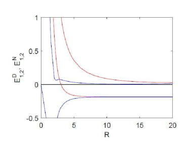
Figure 8: The Dirichlet-Neumann estimate of the spectrum in the critical case for $p=2$.

(RS, , Sec. XIII.15) the possible negative eigenvalues are squeezed between those curves. We see that the bounds become very tight for $R\gtrsim 7$ and indicate the critical problem has for $p=2$ an eigenvalue $E_{1}\approx-0.18365$. Furthermore, $\sigma_{\mathrm{disc}}(L)$ consists of a single point because the second lower (Neumann) estimate is in positive values for $R$ large enough. A similar numerical analysis also suggests the ground state existence for other values of $p$ but it becomes unreliable for $p\gtrsim 20$. We conjecture that the discrete spectrum is nonvoid for all $p>1$ but empty for hyperbolic regions, $p=\infty$.

We are able to get in a numerical way an idea about the ground state eigenfunction, again in the case $p=2$, as plotted in Fig. 9 based on

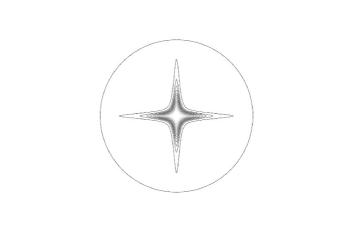
Figure 9: The ground state eigenfunction in the critical case for $p=2$.

solution in the circle with either boundary condition; we note that with the $R=20$ cut-off the Dirichlet and Neumann ones are practically identical which is not surprising since one expects a superexponential decay along the axes. The outer level in the plot marks the $10^{-3}$ value.

5 Resonances in Smilansky-Solomyak model

The models we consider have other interesting properties. Let us return to the setting of Section 2 and show that the system exhibits a rich resonance structure; we refer to ELT17a ; ELT17b for a detailed discussion of these phenomena. To begin with, we have to say which resonances we speak about. There are resolvent resonances associated with poles in the analytic continuation of the resolvent over the cut(s) corresponding to the continuous spectrum, scattering resonances identified with complex singularities of the scattering matrix.

The former are found using the same Jacobi matrix problem as before, of course, this time with a ‘complex energy’. Let is look at the latter. Suppose the incident wave comes in the $m$-th channel from the left. We use the Ansatz

$$f(x,y)=\left\{\begin{array}[]{l}\sum_{n=0}^{\infty}\Big{(}\delta_{mn}\mathrm{e}^{-ipx}\psi_{n}(y)+r_{mn}\,\mathrm{e}^{ix\sqrt{p^{2}+\epsilon_{m}-\epsilon_{n}}}\psi_{n}(y)\Big{)}\\[5.0pt] \sum_{n=0}^{\infty}t_{mn}\,\mathrm{e}^{-ix\sqrt{p^{2}+\epsilon_{m}-\epsilon_{n}}}\psi_{n}(y)\end{array}\right.$$ (26)

for $\mp x>0$, respectively, where $\epsilon_{n}=n+\frac{1}{2}$ and the incident wave energy is assumed to be $p^{2}+\epsilon_{m}=:k^{2}$. It is straightforward to compute from here the boundary values $f(0\pm,y)$ and $f^{\prime}(0\pm,y)$. The continuity requirement at $x=0$ together with the orthonormality of the basis $\{\psi_{n}\}$ yields

$$t_{mn}=\delta_{mn}+r_{mn}.$$ (27)

Furthermore, we substitute the boundary values coming from the Ansatz (26) into

$$f^{\prime}(0+,y)-f^{\prime}(0-,y)-\lambda yf(0,y)=0$$ (28)

and integrate the obtained expression with $\int\mathrm{d}y\,\psi_{l}(y)$. This yields

$$\sum_{n=0}^{\infty}\Big{(}2p_{n}\delta_{ln}-i\lambda(\psi_{l},y\psi_{n})\Big{)}r_{mn}=i\lambda(\psi_{l},y\psi_{m}),$$ (29)

where we have denoted $p_{n}=p_{n}(k):=\sqrt{k^{2}-\epsilon_{n}}$. In particular, poles of the scattering matrix are associated with the kernel of the $\ell^{2}$ operator on the left-hand side. In particular, putting $l=m$ we obtain essentially the same condition we had before, cf. (6) and(7), thus we arrive at the following conclusion:

Proposition 3

The resolvent and scattering resonances coincide in the Smilansky-Solomyak model.

Let us add a few comments:

• The on-shell scattering matrix for the initial momentum $k$ is a $\nu\times\nu$ matrix where $\nu:=\big{[}k^{2}-\frac{1}{2}\big{]}$ whose elements are the transmission and reflection amplitudes; they have common singularities.

• The resonance condition may have (and in fact it has) numerous solutions, but only those ‘not far from the physical sheet’ are of interest.

• The Riemann surface of energy has infinite number of sheets determined by the choices branches of the square roots. The interesting resonances on the $n$-th sheet are obtained by flipping sign of the first $n-1$ of them.

The weak-coupling analysis follows the route as for the discrete spectrum, cf. (LABEL:component)–(11) above; in fact it includes the eigenvalue case if we stay on the ‘first’ sheet. It shows that for small $\lambda$ a resonance poles splits of each threshold according to the asymptotic expansion

$$\mu_{n}(\lambda)=-\frac{\lambda^{4}}{64}\big{(}2n+1+2in(n+1)\big{)}+o(\lambda^{4}).$$ (30)

Hence the distance for the corresponding threshold is proportional to $\lambda^{4}$ and the trajectory asymptote is the ‘steeper’ the larger $n$ is. However, one solve the condition (29) numerically ELT17a . This allows us to go beyond the weak coupling regime and the picture becomes more intriguing as shown in Fig. 10.

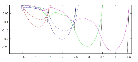
Figure 10: Resonance trajectories as the coupling constant $\lambda$ varies from zero to $\sqrt{2}$.

The picture shows clearly the asymptotes of the resonance trajectories for small values $\lambda$ when the poles split from the channel threshold given by the oscillator eigenvalues. For stronger coupling the behaviour changes and eventually the poles return to the real axis as $\lambda$ approaches the critical value. What is even more interesting, the numerical solutions reveals other, ‘non-threshold’ resonances at the second and third Riemann sheet, indicated by dotted lines, that appear at $\lambda=1.287$ and $\lambda=1.19$, respectively.

6 Concluding remarks

While we have been able to demonstrate many properties of the models under consideration, various mathematical questions remain open, for instance

• in the original Smilansky-Solomyak model and its $\delta^{\prime}$ modification of Sec. 3.3 we know that the essential spectrum is absolutely continuous. We expect that this will also be the case for the models with regular potential channels but this remains to be demonstrated.

• in the regular Smilansky-Solomyak model the ‘escape channel’ may have more than one mode provided $\#\sigma_{\mathrm{disc}}(L)>1$ holds for the operator (13). In this situation it is natural to ask how the spectral multiplicity changes with $\lambda$.

• many question concern resonances in the Smilansky-Solomyak model. One would like to know, inter alia, what is their number in a given part of the complex plane, whether there are resonance free zones for a fixed $\lambda$, or whether all the poles will eventually return to the real axis as $\lambda$ increases. Furthermore, we are interested in the mechanism which produces the ‘non-threshold’ resonances and the coupling constant values at which they appear. Finally, resonance effects are also expected to occur in the regular version of the model.

From the physical point of view the most interesting question concerns the classical motion in the regular model, magnetic and nonmagnetic, as well as in the model of Sec. 4. We have mentioned in the opening of Sec. 3.1 that a step in this direction was made in G18 , however, the importance of the question goes beyond the motivation of that paper dealing with modeling quantum measurements as it may offer a new and interesting insight into the quantum-classical correspondence in unusual situations we have discussed here.

- (1) S. Albeverio, F. Gesztesy, R. Høegh-Krohn, and H. Holden: Solvable Models in Quantum Mechanics, 2nd edition, AMS Chelsea Publishing, Providence, R.I., 2005.
- (2) D. Barseghyan and P. Exner: A regular version of Smilansky model, J. Math. Phys. 55 (2014), 042104.
- (3) D. Barseghyan and P. Exner: A regular analogue of the Smilansky model: spectral properties, Rep. Math. Phys. 80 (2017), 177–192.
- (4) D. Barseghyan and P. Exner: A magnetic version of the Smilansky-Solomyak model, J. Phys. A: Math. Theor. 50 (2017), 485203 (24pp).
- (5) D. Barseghyan, P. Exner, A. Khrabustovskyi, and M. Tater: Spectral analysis of a class of Schrödinger operators exhibiting a parameter-dependent spectral transition, J. Phys. A: Math. Theor. 49 (2016), 165302.
- (6) W. D. Evans and M. Solomyak: Smilansky’s model of irreversible quantum graphs. I: The absolutely continuous spectrum, J. Phys. A: Math. Gen. 38 (2005), 4611–4627.
- (7) W. D. Evans and M. Solomyak: Smilansky’s model of irreversible quantum graphs. II: The point spectrum, J. Phys. A: Math. Gen. 38 (2005), 7661–7675.
- (8) P. Exner and D. Barseghyan: Spectral estimates for a class of Schrödinger operators with infinite phase space and potential unbounded from below, J. Phys. A: Math. Theor. 45 (2012), 075204 (14pp).
- (9) P. Exner and J. Lipovský: Smilansky-Solomyak model with a -interaction, Phys. Lett. A382 (2018), 1207–1213.
- (10) P. Exner, V. Lotoreichik, and M. Tater: Spectral and resonance properties of Smilansky Hamiltonian, Phys. Lett. A381 (2017), 756–761.
- (11) P. Exner, V. Lotoreichik, and M. Tater: On resonances and bound states of Smilansky Hamiltonian, Nanosystems: Phys. Chem. Math. 7 (2016), 789–802.
- (12) L. Geisinger, T. Weidl: Sharp spectral estimates in domains of infinite volume, Rev. Math. Phys. 23 (2011), 615–641.
- (13) I. Guarneri: Irreversible behaviour and collapse of wave packets in a quantum system with point interactions, J. Phys. A: Math. Theor. 44 (2011), 485304 (22 pp).
- (14) I. Guarneri: A model with chaotic scattering and reduction of wave packets, J. Phys. A: Math. Theor. 51 (2018), 095304 (16 pp).
- (15) V. Jakšić, S. Molchanov, and B. Simon: Eigenvalue asymptotics of the Neumann Laplacian of regions and manifolds with cusps, J. Funct. Anal. 106 (1992), 59–79.
- (16) T. Kato: Perturbation theory for linear operators, Springer-Verlag, Berlin, 1995.
- (17) A. Laptev, T. Weidl: Sharp Lieb-Thirring inequalities in high dimensions, Acta Math. 184 (2000), 87–111.
- (18) O. Mickelin: Lieb-Thirring inequalities for generalized magnetic fields, Bull. Math. Sci. 6 (2016), 1–14.
- (19) S. Naboko and M. Solomyak: On the absolutely continuous spectrum in a model of an irreversible quantum graph, Proc. Lond. Math. Soc. (3) 92 (2006), 251–272.
- (20) M. Reed and B. Simon: Methods of modern mathematical physics. II. Fourier Analysis, Self-Adjointness, IV. Analysis of Operators, Academic Press, New York, 1975, 1978.
- (21) G. Rozenblum and M. Solomyak: On a family of differential operators with the coupling parameter in the boundary condition, J. Comput. Appl. Math. 208 (2007), 57–71.
- (22) B. Simon: Some quantum operators with discrete spectrum but classically continuous spectrum, Ann. Phys. 146 (1983), 209–220.
- (23) U. Smilansky: Irreversible quantum graphs, Waves Random Media 14 (2004), S143–S153.
- (24) M. Solomyak: On the discrete spectrum of a family of differential operators, Funct. Anal. Appl. 38 (2004), 217–223.
- (25) M. Solomyak: On a mathematical model of irreversible quantum graphs, St. Petersbg. Math. J. 17 (2006), 835–864.
- (26) M. Solomyak, On the limiting behaviour of the spectra of a family of differential operators, J. Phys. A: Math. Gen. 39 (2006), 10477–10489.
- (27) M. Znojil, Quantum exotic: a repulsive and bottomless confining potential, J. Phys. A: Math. Gen. 31 (1998), 3349–3355.