Emergence of pure spin current in doped excitonic magnets

Abstract

An excitonic magnet hosts a condensate of spin-triplet excitons composed of conduction-band electrons and valence-band holes, and may be described by the two-orbital Hubbard model. When the Hamiltonian has the nearest-neighbor interorbital hopping integrals with $d$-wave symmetry and the number of electrons is slightly away from half filling, the $\bm{k}$-space spin texture appears in the excitonic phase with a broken time-reversal symmetry. We then show that, applying electric field to this doped excitonic magnet along a particular direction, a pure spin current emerges along its orthogonal direction. We discuss possible experimental realization of this type of the pure spin current in actual materials.

I Introduction

In a pure spin current, the flow of electrons with up-spin goes along the opposite direction to that with down-spin and the net charge current is absent. Generation of the pure spin current is one of the key issues in spintronics applications. Although in the past the spin-Hall effect Maekawa2013JPSJ ; Sinova2015RMP in nonmagnetic materials composed of heavy atoms with a strong spin-orbit coupling is employed for this purpose, it has recently been suggested that, even in the case where the spin-orbit coupling is negligible, the pure spin current can be induced in antiferromagnetically ordered systems, such as noncolinear antiferromagnets Zelezny2017PRL ; Zhang2018NJP ; Kimata2019Nature and organic colinear antiferromagnets with a broken glide symmetry Naka2019NC .

In this paper, we will show that the pure spin current can also be generated in a spin-triplet excitonic phase (EP), where the electrons in the valence band and holes in the conduction band form spin-triplet pairs by attractive Coulomb interaction, and condense into a state with quantum coherence at low temperatures. Kuneš and Geffroy Kunes2016PRL used a doped two-orbital Hubbard model with cross-hopping integrals, i.e., the nearest-neighbor hopping terms between different orbitals, and showed that the $\bm{k}$-space spin texture emerges in the spin-triplet EP. They found that the symmetry of the spin texture depends on the symmetry of the cross-hopping integrals; in particular, when the symmetry of the cross-hopping terms is $p$-wave, an orbital off-diagonal component of the global spin current becomes finite in the EP. However, unfortunately, the net spin current must be zero in an equilibrium state Geffroy2018PRB ; Nishida2019PRB , just as the Bloch’s theorem claims the absence of any spontaneous currents Ohashi1996JPSJ .

To extract the pure spin current in excitonic magnets, an external field must be applied to the system. We focus on the case where the cross-hopping integrals have the $d$-wave symmetry. In this case, after the EP transition, the state loses the time-reversal symmetry, while the net magnetization is zero Kunes2016PRL . As a result, the pure spin current is expected to emerge when an external electric field is applied.

The rest of this paper is organized as follows. In Sec. II, we introduce the two-orbital Hubbard model with the $d$-wave cross-hopping terms defined on the two-dimensional square lattice, and give the definition of the excitonic order parameter. The electric and Hall conductivities obtained from the linear response theory are also introduced in this section. In Sec. III, we calculate the spin currents generated in the EP by varying the interaction parameters and density of electrons. Possible experimental realization of the pure spin current in doped excitonic magnets is also discussed in this section. A summary of our results is given in Sec. IV. Appendices are given to discuss details of the mean-field analysis of the Hamiltonian and the current-current correlation function used.

II Model and method

II.1 Hamiltonian

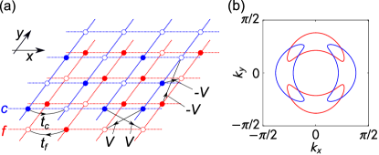
Figure 1: (a) Schematic representation of the kinetic term of the two-orbital Hubbard model with $d$-wave cross-hopping integrals [see Eq. (2) in the main text]. The red (blue) circles indicate the $f$ ($c$) orbital. (b) Calculated $\bm{k}$-space spin texture with the $d$-wave symmetry in the spin-triplet EP away from half filling. The red (blue) lines denote the Fermi surfaces for up (down) spin. The interaction strengths are set to be $U=9.5$, $U^{\prime}=5.0$, and $J=J^{\prime}=0$, and the density of electrons is set to be $N=1.92$.

We consider the two-orbital Hubbard model defined on the two-dimensional square lattice, where we include the cross hopping integrals as well as the standard nearest-neighbor hopping integrals Kunes2014PRB1 ; Kunes2014PRB2 ; Kunes2016PRL . The Hamiltonian is written as

$$\mathcal{H}=\mathcal{H}_{0}+\mathcal{H}_{\mathrm{int}}$$ (1)

with the kinetic term

$$\mathcal{H}_{0} =\sum_{j,\tau,\sigma}\left(t_{c}c^{\dagger}_{j+\tau,\sigma}c_{j,\sigma}+t_{f}f_{j+\tau,\sigma}^{\dagger}f_{j,\sigma}+\mathrm{H.c.}\right)$$

$$+\sum_{j,\tau,\sigma}\left(V_{1,\tau}c^{\dagger}_{j+\tau,\sigma}f_{j,\sigma}+V_{2,\tau}f^{\dagger}_{j+\tau,\sigma}c_{j,\sigma}+\mathrm{H.c.}\right)$$

$$+\frac{D}{2}\sum_{j,\sigma}\left(n^{c}_{j,\sigma}-n^{f}_{j,\sigma}\right)$$ (2)

and the interaction term

$$\mathcal{H}_{\mathrm{int}} =\frac{U}{2}\sum_{i,\sigma}\left(f_{i,\sigma}^{\dagger}f_{i,\sigma}f_{i,-\sigma}^{\dagger}f_{i,-\sigma}+c_{i,\sigma}^{\dagger}c_{i,\sigma}c_{i,-\sigma}^{\dagger}c_{i,-\sigma}\right)$$

$$+U^{\prime}\sum_{i,\sigma,\sigma^{\prime}}f_{i,\sigma}^{\dagger}f_{i,\sigma}c_{i,\sigma^{\prime}}^{\dagger}c_{i,\sigma^{\prime}}-J\sum_{i,\sigma,\sigma^{\prime}}f_{i,\sigma}^{\dagger}f_{i,\sigma^{\prime}}c_{i,\sigma^{\prime}}^{\dagger}c_{i,\sigma}$$

$$+\frac{J^{\prime}}{2}\sum_{i,\sigma}\left(f_{i,\sigma}^{\dagger}c_{i,\sigma}f_{i,-\sigma}^{\dagger}c_{i,-\sigma}+c_{i,\sigma}^{\dagger}f_{i,\sigma}c_{i,-\sigma}^{\dagger}f_{i,-\sigma}\right),$$ (3)

where $c_{i,\sigma}^{\dagger}$ ($f_{i,\sigma}^{{\dagger}}$) and $c_{i,\sigma}$ ($f_{i,\sigma}$) are the creation and annihilation operators of an electron on the conduction-band orbital $c$ (valence-band orbital $f$) at site $j$ with spin $\sigma$, and $n^{c}_{j,\sigma}$ ($n^{f}_{j,\sigma}$) is the electron number operator on the $c$ ($f$) orbital at site $j$ with spin $\sigma$. In Eq. (2), $D$ is the on-site energy-level splitting, $t_{c}$ and $t_{f}$ are the hopping integrals between the same orbitals on the nearest-neighbor sites, $V_{1,\tau}$ and $V_{2,\tau}$ are the hopping integrals between the different orbitals on the nearest-neighbor sites (which are referred to as the cross-hopping integrals), and $\tau$ denotes the primitive translation vector $\bm{a}_{\tau}$. For the cross-hopping integrals with the $d$-wave symmetry, we assume $V_{1,x}=V_{2,x}=V_{1,-x}=V_{2,-x}=V$ and $V_{1,y}=V_{2,y}=V_{1,-y}=V_{2,-y}=-V$, where $-\tau$ denotes the primitive translation vector of an opposite sign, i.e., $\bm{a}_{-\tau}=-\bm{a}_{\tau}$. The kinetic term is schematically illustrated in Fig. 1(a). In Eq. (3), $U$, $U^{\prime}$, $J$, and $J^{\prime}$ represent the intraorbital Coulomb interaction, interorbital Coulomb interaction, Hund’s rule coupling, and pair hopping, respectively.

We assume the periodic boundary condition. Then, the Fourier transformation of Eq. (2) reads

$$\mathcal{H}_{0}=\sum_{k,\sigma}\biggl{[}{\varepsilon}_{c}(\bm{k}){c}_{{\bm{k}},\sigma}^{\dagger}{c}_{{\bm{k}},\sigma}+{\varepsilon}_{f}(\bm{k}){f}_{{\bm{k}},\sigma}^{\dagger}{f}_{{\bm{k}},\sigma}\\ +\left({\gamma}(\bm{k}){c}_{{\bm{k}},\sigma}^{\dagger}{f}_{{\bm{k}},\sigma}+\mathrm{H.c}\right)\biggr{]},$$ (4)

where

$${\varepsilon}_{c}(\bm{k}) =2t_{c}\sum_{\tau}\cos{k_{\tau}}+\frac{D}{2},$$ (5)

$${\varepsilon}_{f}(\bm{k}) =2t_{f}\sum_{\tau}\cos{k_{\tau}}-\frac{D}{2},$$ (6)

and

$$\gamma(\bm{k})=2V\left(\cos{k_{x}}-\cos{k_{y}}\right)$$ (7)

with $k_{\tau}={\bm{k}}\cdot\bm{a}_{\tau}$. Hereafter, we assume the hopping integrals as $-t_{c}=t_{f}=1$ (direct gap and the unit of energy), which leads to a uniform excitonic order. We set $D=6$, $V=0.1$, and the lattice constant to be unity ($\left|\bm{a}_{\tau}\right|=1$) throughout the paper.

II.2 Order parameters

We assume the spin-triplet excitonic order of the spin direction along $z$-axis. Note that the energy of the spin-singlet excitonic order is strictly equal to that of the spin-triplet excitonic order if the Hund’s rule coupling is absent and that the finite Hund’s rule coupling stabilizes the spin-triplet excitonic order Kaneko2014PRB . We do not consider the spin-singlet excitonic order here, which may be stabilized in the presence of strong electron-phonon coupling terms Kaneko2015PRB .

Since the present model has a direct gap, we ignore any excitonic density-wave states. We instead consider the uniform spin-triplet excitonic order, of which the order parameter is defined as

$$\Phi^{\mathrm{t}}=|\Phi^{\mathrm{t}}|e^{i\phi}=\frac{1}{L^{2}}\sum_{j,\sigma}\sigma\left\langle{c}_{j,\sigma}^{\dagger}{f}_{j,\sigma}\right\rangle,$$ (8)

where $\phi$ is the phase of the complex order parameter, $\sigma=1$ ($-1$) indicates the up (down) spin, and $L^{2}$ is the number of sites in the system. We apply the mean-field approximation to the Hamiltonian (see Appendix A) and solve the self-consistent equations to obtain the order parameter. The representative $d$-wave spin texture in the EP at a hole-doped region is illustrated in Fig. 1(b). We find that the Fermi surfaces for each spin are anisotropic, implying that the time-reversal symmetry, which exists in the original Hamiltonian, is apparently broken in the EP.

In the definition of the spin-triplet excitonic order parameter, we assume that the real and imaginary parts of the order parameter point along the same direction. However, we should note that there is no restriction to the relative direction between them, except for the case where the pair hopping, which makes the order parameter real Kaneko2015PRB , is present. Since the aim of our study is to discuss the spin current generated in the excitonic phase with $\bm{k}$-space spin texture, we restrict ourselves to considering such a definition, as in Ref. Nishida2019PRB , for simplicity.

We also consider the competition between the EP and antiferromagnetic (AFM) phase Kaneko2012PRB . The AFM order parameter is defined as

$$m_{\ell}=\frac{1}{L^{2}}\sum_{j,\sigma}\sigma e^{-i\bm{Q}\cdot\bm{r}_{j}}\left\langle{\ell}_{j,\sigma}^{\dagger}{\ell}_{j,\sigma}\right\rangle,$$ (9)

where $\ell$ ($=c,f$) is an orbital index, $\bm{r}_{j}$ is the position of site $j$, and $\bm{Q}=(\pi,\pi)$ is a checkerboard-type AFM ordering vector.

Even though the mean-field approximation used here is not sufficient in intermediate or strong coupling regime, it is suitable for obtaining the excitonic ground state with $\bm{k}$-space spin texture. This is because any symmetry breaking of the system can in principle be described in this approximation, irrespective of its coupling strength. For simplicity, we neglect other possible phases such as incommensurate spin-density waves and superconductivity here. The statistical average $\left\langle\cdots\right\rangle$ is taken at absolute zero temperature. The computations are performed with $L^{2}=400^{2}$.

II.3 Charge and spin currents

We introduce the external electric field via the Peierls phase. The electron operators are then changed as

$$\ell_{j,\sigma}\rightarrow e^{i\bm{A}\cdot\bm{r}_{j}}\ell_{j,\sigma},$$ (10)

where $\bm{A}$ is a vector potential. The speed of light $c$, reduced Planck constant $\hbar$, and elementary charge $e$ are all set to unity. We assume a spatially uniform vector potential. Only the hopping terms in the kinetic term of the Hamiltonian are modified by the Peierls substitution. The electric current operator may be defined as

$$\bm{j}=-\left.\frac{\partial\mathcal{H}(\bm{A})}{\partial\bm{A}}\right|_{\bm{A}=0}=\sum_{\sigma}\bm{j}_{\sigma},$$ (11)

where

$$\bm{j}_{\sigma}=i\sum_{j,\tau}\bm{a}_{\tau}\Bigl{[}\left(t_{c}c^{\dagger}_{j+\tau,\sigma}c_{j,\sigma}+t_{f}f_{j+\tau,\sigma}^{\dagger}f_{j,\sigma}\right)\\ +\left(V_{1,\tau}c^{\dagger}_{j+\tau,\sigma}f_{j,\sigma}+V_{2,\tau}f^{\dagger}_{j+\tau,\sigma}c_{j,\sigma}\right)\Bigr{]}+\mathrm{H.c.}$$ (12)

indicates the current of the conduction electrons with spin $\sigma$. If the system shows a real-space spin texture Loss1990PRL or the Hamiltonian has spin-orbit interaction terms Shi2006PRL , the spin current should be defined as a second-rank pseudotensor given by the flow direction of electron spin and the orientation of the spin. These effects are not included in our model, and we assume that both the real and imaginary parts of the spin-triplet excitonic order parameter point along $z$-axis. Hence, we can simply define a spin current as $\bm{j}_{\mathrm{s}}=\bm{j}_{\uparrow}-\bm{j}_{\downarrow}$. We call the electric current a charge current $\bm{j}_{\mathrm{c}}=\bm{j}_{\uparrow}+\bm{j}_{\downarrow}$.

II.4 Conductivity

We carry out the calculation of the spin and charge currents within the linear response theory, where the response function with regard to the applied external field can be obtained from the equilibrium state. This implies that the external field is assumed to be weak enough, so that the order parameter is not affected. The Hamiltonian is expanded with respect to $\bm{A}$ as Jaklic2000AP

$$\mathcal{H}(\bm{A})=\mathcal{H}(0)-\bm{j}\cdot\bm{A}-\frac{1}{2}\bm{A}\cdot\underline{u}\bm{A}+\mathcal{O}\left(\left|\bm{A}\right|^{3}\right),$$ (13)

where

$$u_{\alpha\beta}=\sum_{j,\tau,\sigma}a^{(\alpha)}_{\tau}a^{(\beta)}_{\tau}\Bigl{[}\left(t_{c}c^{\dagger}_{j+\tau,\sigma}c_{j,\sigma}+t_{f}f_{j+\tau,\sigma}^{\dagger}f_{j,\sigma}\right)\\ +\left(V_{1,\tau}c^{\dagger}_{j+\tau,\sigma}f_{j,\sigma}+V_{2,\tau}f^{\dagger}_{j+\tau,\sigma}c_{j,\sigma}\right)\Bigr{]}+\mathrm{H.c.}$$ (14)

is the $\alpha\beta$ component of a stress tensor. We denote $a^{(\alpha)}_{\tau}$ as the $\alpha$-component of $\bm{a}_{\tau}$.

The electric field is given by $\bm{E}=-\frac{\partial\bm{A}}{\partial t}$. From the linear response theory, the optical conductivity tensor as a function of the frequency $\omega$ of the electric field may be given as Jaklic2000AP

$$\sigma_{\alpha\beta}(\omega^{+})=\frac{1}{L^{2}}\frac{i\left[\chi^{\mathrm{R}}_{\alpha\beta}(\omega^{+})-\langle u_{\alpha\beta}\rangle\right]}{\omega^{+}}$$ (15)

with a retarded current-current correlation function

$$\chi^{\mathrm{R}}_{\alpha\beta}(\omega^{+})=-i\int^{\infty}_{0}\mathrm{d}t\,e^{i\omega^{+}t}\left\langle\left[j^{(\alpha)}(t),j^{(\beta)}\right]\right\rangle,$$ (16)

where $\omega^{+}=\omega+i\eta$ (with a positive infinitesimal value $\eta$) and $j^{(\alpha)}(t)=e^{i\mathcal{H}t}j^{(\alpha)}e^{-i\mathcal{H}t}$. The explicit form of $\chi^{\mathrm{R}}_{\alpha\beta}(\omega^{+})$ in the mean-field approximation is given in Appendix B. The Drude weight tensor defined by

$$D_{\alpha\beta}=\frac{\pi}{L^{2}}\left(\mathrm{Re}\,\chi^{\mathrm{R}}_{\alpha\beta}(0)-\left\langle u_{\alpha\beta}\right\rangle\right)$$ (17)

may be separated into contributions from the up-spin and down-spin electrons, i.e.,

$$D_{\alpha\beta}=\sum_{\sigma}D_{\alpha\beta}(\sigma),$$ (18)

where $D_{\alpha\beta}(\sigma)$ corresponds to the electric-field response of the spin-$\sigma$ current. The static conductivity is equal to the real part of the optical conductivity at $\omega=0$. In actual materials, there are defects and impurities, which scatter the moving electrons. If the scattering rate is approximated to be a constant $\Gamma$, the conductivity tensor may be given by Sugimoto2014PRB

$$\mathrm{Re}\,\sigma_{\alpha\beta}(0)=\frac{D_{\alpha\beta}}{\pi\Gamma}.$$ (19)

When the direction $\alpha$ is parallel (perpendicular) to the direction $\beta$, Eq. (19) represents the electric (Hall) conductivity.

III Results of calculation

III.1 Pure spin current

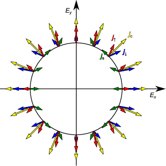
Figure 2: Calculated electric-field-angle dependence of the average values of up-spin current $\bm{j}_{\uparrow}$ (red arrows), down-spin current $\bm{j}_{\downarrow}$ (blue arrows), charge current $\bm{j}_{\mathrm{c}}$ (yellow arrows), and spin current $\bm{j}_{\mathrm{s}}$ (green arrows), in the case where the $\bm{k}$-space spin texture with the $d$-wave symmetry is present. The charge current is always parallel to the applied electric field. The parameters are set to be the same as used in Fig. 1(b).

The calculated result for the field-angle dependence of the charge and spin currents in the hole-doped ($N=1.92$) spin-triplet EP with the $d$-wave spin texture is illustrated in Fig. 2. We find that, reflecting the broken time-reversal symmetry, the spin currents are nonzero in any field angles. We also find that, when the electric field is along the diagonal direction of the square lattice, the spin current runs along the direction perpendicular to the electric field, while the charge current is parallel to the electric field. This result clearly indicates that the pure spin current is obtained in the doped excitonic magnet when the electric field is applied along the diagonal direction of the square lattice. In other words, the excitonic magnets with the broken time-reversal symmetry can host the pure spin current.

We denote the electric and Hall components of the Drude-weight tensor with spin $\sigma$ as $D_{\parallel}(\sigma)$ and $D_{\perp}(\sigma)$, respectively. In the rest of this section, the direction of the electric field is fixed to the $(1,1)$ direction of the square lattice, so that we have the identity $D_{\perp}(\uparrow)=-D_{\perp}(\downarrow)$. We define the conversion rate of the spin current to the charge current as $\beta=\left|D_{\perp}(\uparrow)/D_{\parallel}(\uparrow)\right|$. The spin current is present when $\beta\neq 0$, and the value of $\beta$ indicates the generation efficiency of the pure spin current with respect to the applied electric field.

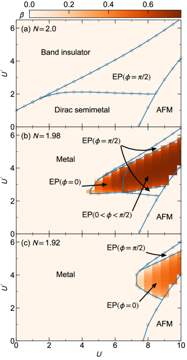
Figure 3: Calculated phase diagrams of the two-orbital Hubbard model at (a) $N=2$, (b) $N=1.98$, and (c) $N=1.92$ in the $(U,U^{\prime})$ plane, where we set $J=J^{\prime}=0$. The intensity contour plots indicates the conversion rate $\beta$.

III.2 The case of $J=J^{\prime}=0$

First, let us discuss the case where the Hund’s rule coupling and pair hopping term are both absent, i.e., $J=J^{\prime}=0$ in Eq. (3). It is known that the system at half filling ($N=2$) without the cross-hopping terms is AFM when $U\gg U^{\prime}$, while it is band insulating when $U^{\prime}\gg U$, and that the EP emerges between these two phases Kaneko2012PRB .

The EP remains even if the cross-hopping terms are introduced. The phase of the excitonic order parameter is fixed to $\phi=\pi/2$ when the cross-hopping integrals have the $d$-wave symmetry. Figure 3(a) shows the phase diagram of the two-orbital model with the $d$-wave cross-hopping terms at half-filling. The cross-hopping terms yield the Dirac-cone band dispersions in the noninteracting bands Young2015PRL , so that the four different phases appear in the $U$-$U^{\prime}$ phase diagram at half-filling; i.e., the band insulating phase, normal semimetallic phase, EP with $\phi=\pi/2$, and the AFM phase.

As holes are slightly doped into the system, the new EP with $0\leq\phi<\pi/2$ appears. Figure 3(b) shows the phase diagram at $N=1.98$. We find that upon doping the $\bm{k}$-space spin texture immediately appears in the Fermi surface, which leads to the emergence of the spin current. Note that the k-space spin texture (or the spin current) is originated from the cooperation of the EP transition and cross-hopping integrals and that the spin current remains even when $\phi=0$ in the hole-doped region. However, when $\phi=\pi/2$, the $\bm{k}$-space spin texture disappears in the Fermi surface [9], so that the spin current is no longer observed. Figure 3(c) shows the phase diagram at $N=1.92$. As the doping rate increases, the EP with $0<\phi<\pi/2$ disappears.

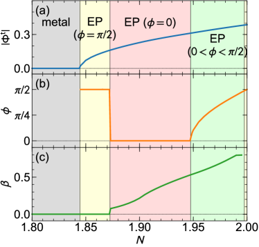
Figure 4: (a) Calculated magnitude of the excitonic order parameter $|\Phi^{\textrm{t}}|$, (b) its phase $\phi$, and (c) conversion rate $\beta$ as a function of the electron density $N$. Interaction strengths are set to $U=9.5$, $U^{\prime}=5.0$, and $J=J^{\prime}=0$.

The excitonic order parameter and conversion rate as a function of the electron density at $U=9.5$ and $U^{\prime}=5.0$ are illustrated in Fig. 4. Both the order parameter and conversion rate monotonically decrease as the density of doped holes increases. We find that, when the $\bm{k}$-space spin texture disappears (or equivalently $\beta=0$), the EP with $\phi=\pi/2$ is stabilized. In the over-doped region, the EP completely vanishes, and the system becomes normal metallic.

III.3 The case of finite $J$ and $J^{\prime}$

Next, to be more realistic, let us take into account the Hund’s rule coupling and pair-hopping terms. We assume the relations $U^{\prime}=U-2J$ and $J=J^{\prime}$ in this subsection. It is known that the pair-hopping terms force the phase of the excitonic order parameter to be zero Kaneko2015PRB .

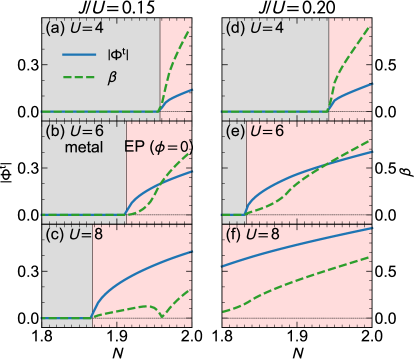
Figure 5: Calculated excitonic order parameters $|\Phi^{\mathrm{t}}|$ (blue solid lines) and conversion rate $\beta$ (green dashed lines) as a function of the electron density $N$. We assume $J/U=0.15$ in (a)-(c) and $J/U=0.20$ in (d)-(f), and $U=4$ in (a) and (d), $U=6$ in (b) and (e), and $U=8$ in (c) and (f).

Figure 5 shows the calculated results for the excitonic order parameter and conversion rate as a function of the electron density. We find that the spin current appears even when finite $J$ and $J^{\prime}$ are present. However, the conversion rate is not proportional to the excitonic order parameter because the rate is not determined by the magnitude of the order but is determined by the degree of the spin splitting in the $\bm{k}$-space spin texture. We note that the AFM phase is not stabilized in the parameter region shown in Fig. 5.

III.4 Possible realization of the pure spin current

Finally, let us discuss possible experimental realization of the spin current in actual materials. A number of transition-metal oxides have been regarded as candidates for the excitonic magnets. For example, some kinds of cobalt oxides with the $d^{6}$ electron configuration were suggested to be the spin-triplet excitonic magnets Kunes2014PRL ; Yamaguchi2017JPSJ ; Yamaguchi2018PB ; Moyoshi2018PRB ; Tomiyasu2018AQT , where the electrons in the $e_{g}$ orbitals and holes in the $t_{2g}$ orbitals form excitonic pairs. Also, Ca₂RuO₄ with the $d^{4}$ electron configuration was suggested to be an excitonic magnet Khaliullin2013PRL ; Akbari2014PRB ; Jain2017NP . However, unfortunately, no experimental observations of the spin texture have so far been reported in these materials.

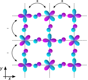
Figure 6: Schematic picture of the orbital pattern leading to the $\bm{k}$-space spin texture with the $d$-wave symmetry in the EP. Note that the tilting of the ligand $p$ orbitals makes the cross-hopping integrals be of the $d$-wave symmetry.

In order to realize excitonic magnets with $\bm{k}$-space spin texture of the $d$-wave symmetry, we may focus on transition-metal oxides with the layered perovskite structure. Figure 6 illustrates an orbital pattern, which leads to the cross-hopping integrals of the $d$-wave symmetry. To make the direct-gap band dispersions in the square lattice, we may assume that the one band comes from the $d_{xy}$ orbitals and the other comes from the $d_{x^{2}-y^{2}}$ (or $d_{3z^{2}-r^{2}}$) orbitals. This is because the nearest-neighbor hopping integrals between the $d_{xy}$ orbitals are positive, while those between the $d_{x^{2}-y^{2}}$ orbitals are negative Slater1954PR . Note that the cross-hopping integrals between the $d_{xy}$ and $d_{x^{2}-y^{2}}$ orbitals via the tilted $p$ orbitals on ligand oxygen ions may have the $d$-wave symmetry (see Fig. 6). Thus, we may suggest a possible experimental realization of the pure spin current in such transition-metal oxides with the layered perovskite structure.

IV Conclusions

We have studied the pure spin current in the doped excitonic magnets, which is generated by applying the external electric field. The two-orbital Hubbard model defined on the two-dimensional square lattice with the cross-hopping integrals of the $d$-wave symmetry was solved in the mean-field approximation. We thus found that the $\bm{k}$-space spin texture emerges in the spin-triplet EP when the holes are slightly doped. Since the spin texture breaks the time-reversal symmetry, we found that the pure spin current is generated along the orthogonal direction of the charge current when the electric field is applied parallel to the diagonal direction of the square lattice.

We also obtained the phase diagrams of the two-orbital Hubbard model by varying the intra- and inter-orbital interactions. We found that the pure spin current emerges in slightly hole-doped EP, which is however suppressed by the excess hole doping. When the phase of the excitonic order parameter becomes $\phi=\pi/2$, the spin texture disappears and consequently the spin current vanishes. We also investigated the case where the Hund’s rule coupling and pair-hopping terms are present and confirmed that the pure spin current can exist in such realistic cases as well. We suggested that some kinds of $3d$ transition-metal oxides with the layered perovskite structure may host the pure spin current driven by the excitonic order, of which the experimental studies are desired.

We want to emphasize that the spin current discussed in this paper is induced purely from the effects of electron correlations. Thus, we found a route to generate the pure spin current in correlated electron systems without the spin-orbit coupling.

Appendix A Mean-field Hamiltonian

First, let us introduce the expectation value defined as

$$n^{\ell\ell^{\prime}}_{\bm{q}}=\sum_{\sigma}n^{\ell\ell^{\prime}}_{\bm{q},\sigma}=\frac{1}{L^{2}}\sum_{\bm{k},\sigma}\left\langle\ell_{\bm{k},\sigma}^{\dagger}\ell^{\prime}_{\bm{k}+\bm{q},\sigma}\right\rangle,$$ (20)

and denote $\bar{c}=f$ and $\bar{f}=c$. Thereby, $n^{cc}_{0}$ and $n^{ff}_{0}$ represent the numbers of electrons on the $c$ and $f$ orbitals per site, respectively.

The mean-field Hamiltonian of the two-orbital Hubbard model may then be obtained as

$$\mathcal{H}^{\rm MF}=\mathcal{H}_{0}+\mathcal{H}_{\mathrm{int}}^{\rm MF},$$ (21)

where

$$\mathcal{H}_{\mathrm{int}}^{\rm MF}=\sum_{\bm{k},\bm{q},\sigma}\biggl{[}\tilde{n}^{cc}_{\bm{q},\sigma}{c}_{{\bm{k}}+\bm{q},\sigma}^{\dagger}{c}_{{\bm{k}},\sigma}+\tilde{n}^{ff}_{\bm{q},\sigma}{f}_{{\bm{k}}+\bm{q},\sigma}^{\dagger}{f}_{{\bm{k}},\sigma}\\ +\tilde{n}^{fc}_{\bm{q},\sigma}{c}_{{\bm{k}}+\bm{q},\sigma}^{\dagger}{f}_{{\bm{k}},\sigma}+\tilde{n}^{cf}_{\bm{q},\sigma}{f}_{{\bm{k}}+\bm{q},\sigma}^{\dagger}{c}_{{\bm{k}},\sigma}\biggr{]}+L^{2}\epsilon_{0}$$ (22)

with

$$\tilde{n}^{\ell\ell}_{\bm{q},\sigma} =Un^{\ell\ell}_{\bm{q},-\sigma}+U^{\prime}n^{\bar{\ell}\bar{\ell}}_{\bm{q}}-Jn^{\bar{\ell}\bar{\ell}}_{\bm{q},\sigma},$$ (23)

$$\tilde{n}^{\ell\bar{\ell}}_{\bm{q},\sigma} =-U^{\prime}n_{\bm{q},\sigma}^{\ell\bar{\ell}}+J\Phi_{\bm{q}}^{\ell\bar{\ell}}+J^{\prime}n^{\bar{\ell}\ell}_{\bm{q},-\sigma},$$ (24)

and

$$\epsilon_{0}= -\frac{U}{2}\sum_{\sigma,\bm{q}}\left[n^{ff}_{\bm{q},-\sigma}\left(n^{ff}_{\bm{q},\sigma}\right)^{*}+n^{cc}_{\bm{q},-\sigma}\left(n^{cc}_{\bm{q},\sigma}\right)^{*}\right]$$

$$-U^{\prime}\sum_{\bm{q}}\left[\left(n^{ff}_{\bm{q}}\right)^{*}n^{cc}_{\bm{q}}-\sum_{\sigma}\left(n_{\bm{q},\sigma}^{cf}\right)^{*}n_{\bm{q},\sigma}^{cf}\right]$$

$$+J\sum_{\bm{q}}\left[\sum_{\sigma}\left(n^{ff}_{\bm{q},\sigma}\right)^{*}n^{cc}_{\bm{q},\sigma}-\left(n_{\bm{q}}^{cf}\right)^{*}n_{\bm{q}}^{cf}\right]$$

$$-\frac{J^{\prime}}{2}\sum_{\sigma,\bm{q}}\left[\left(n^{cf}_{\bm{q},\sigma}\right)^{*}n^{fc}_{\bm{q},-\sigma}+\left(n^{fc}_{\bm{q},\sigma}\right)^{*}n^{cf}_{\bm{q},-\sigma}\right].$$ (25)

A.1 Spin-triplet excitonic order

The order parameter for the uniform spin-triplet excitonic condensation may be written as

$$\Phi^{\mathrm{t}}=\sum_{\sigma}\sigma n^{cf}_{\bm{q}=0,\sigma},$$ (26)

where we assume that the terms with $\bm{q}\neq 0$ vanish in the uniform EP. Diagonalizing the $2\times 2$ mean-field Hamiltonian matrix, we obtain a quasiparticle operator $\alpha_{\bm{k},\sigma,\epsilon}^{\dagger}$ for the band $\epsilon$, which creates a quasiparticle with energy $E^{\epsilon}_{\bm{k},\sigma}$. The quasiparticle operators satisfy $\mathcal{H}^{\rm{MF}}=\sum_{\bm{k},\sigma}\sum_{\epsilon}E^{\epsilon}_{\bm{k},\sigma}\alpha^{\dagger}_{\bm{k},\sigma,\epsilon}\alpha_{\bm{k},\sigma,\epsilon}+L^{2}\epsilon_{0}$ and $\ell_{\bm{k},\sigma}=\sum_{\mu}\psi_{\ell;\epsilon}(\bm{k},\sigma)\alpha_{\bm{k},\sigma,\epsilon}$. The chemical potential $\mu$ is determined from the equation

$$N=\frac{1}{L^{2}}\sum_{{\bm{k}},\sigma}\left[f(E_{\bm{k},\sigma}^{+})+f(E_{\bm{k},\sigma}^{-})\right]$$ (27)

and the order parameter is obtained by solving the self-consistent equation

$$\Phi^{\mathrm{t}}=\frac{1}{L^{2}}\sum_{{\bm{k}},\sigma,\epsilon}\psi^{*}_{c;\epsilon}\psi_{f;\epsilon}f(E_{\bm{k},\sigma}^{\epsilon}),$$ (28)

where we define the Fermi distribution function as $f(E_{\bm{k},\sigma}^{\pm})=\langle{\hat{\alpha}}_{\bm{k},\sigma,\pm}^{\dagger}{\hat{\alpha}}_{\bm{k},\sigma,\pm}\rangle=1/\left(1+e^{\beta\left(E_{\bm{k},\sigma}^{\pm}-\mu\right)}\right)$ with the reciprocal temperature $\beta$. Details of the mean-field calculation of the two-orbital Hubbard model are given in Ref. Nishida2019PRB .

A.2 AFM order

The order parameter for the AFM state may be written as

$$m_{\ell}=\sum_{\sigma}\sigma n^{\ell\ell}_{\bm{Q},\sigma}$$ (29)

with $\bm{Q}=(\pi,\pi)$. The $\bm{k}$-summation over the Brillouin zone was rewritten as $\sum_{\bm{k}}\rightarrow\sum_{\bm{k}_{0}}\sum_{m=0,1}$ with $\bm{k}\rightarrow\bm{k}_{0}+m\bm{Q}$, where the sum of $\bm{k}_{0}$ was taken over the reduced AFM Brillouin zone. Diagonalizing the $4\times 4$ mean-field Hamiltonian matrix for each wave vector and spin, we obtain a quasiparticle operator $\alpha_{\bm{k}_{0},\sigma,\epsilon}^{\dagger}$ for the band $\epsilon$, which creates a quasiparticle with energy $E^{\epsilon}_{\bm{k}_{0},\sigma}$. The quasiparticle operators satisfy $\mathcal{H}^{\rm{MF}}=\sum_{\bm{k}_{0},\sigma}\sum_{\epsilon}E^{\epsilon}_{\bm{k}_{0},\sigma}\alpha^{\dagger}_{\bm{k}_{0},\sigma,\epsilon}\alpha_{\bm{k}_{0},\sigma,\epsilon}+L^{2}\epsilon_{0}$ and $\ell_{\bm{k}_{0}+m\bm{Q},\sigma}=\sum_{\mu}\psi_{\ell,m;\epsilon}(\bm{k}_{0},\sigma)\alpha_{\bm{k}_{0},\sigma,\epsilon}$. The chemical potential is determined from the equation $N=(1/L^{2})\sum_{{\bm{k}}_{0},\sigma,\epsilon}f(E_{\bm{k}_{0},\sigma}^{\epsilon})$ and the order parameter is obtained by solving the self-consistent equations.

Appendix B Current-current correlation function

Using the results of the mean-field approximation given in Appendix A, we obtain the current operator as

$$\bm{j}=\sum_{\bm{k}_{0},\sigma}\sum_{\epsilon,\epsilon^{\prime}}\bm{J}_{\epsilon,\epsilon^{\prime}}(\bm{k}_{0},\sigma)\alpha^{\dagger}_{\bm{k}_{0},\sigma,\epsilon}\alpha_{\bm{k}_{0},\sigma,\epsilon^{\prime}}$$ (30)

with

$$\bm{J}_{\epsilon,\epsilon^{\prime}}(\bm{k}_{0},\sigma)=i\sum_{m}\sum_{\tau}\sum_{\ell,\ell^{\prime}}\bm{a}_{\tau}t_{\ell\ell^{\prime}}(\tau)\\ \times e^{-i(\bm{k}_{0}+m\bm{Q})\cdot\bm{a}_{\tau}}\psi^{*}_{\ell,m;\epsilon}(\bm{k}_{0},\sigma)\psi_{\ell^{\prime},m;\epsilon^{\prime}}(\bm{k}_{0},\sigma),$$ (31)

where we define $t_{\ell\ell}(\tau)=t_{\ell}$, $t_{cf}(\tau)=V_{1,\tau}$ and $t_{fc}(\tau)=V_{2,\tau}$.

Using the matrix elements of the current operator, we obtain the current-current correlation function as

$$\chi^{\mathrm{R}}_{\alpha\beta}(\omega^{+})=\sum_{\bm{k}_{0},\sigma}\sum_{\epsilon,\epsilon^{\prime}}\frac{f(E^{\epsilon}_{\bm{k}_{0},\sigma})-f(E^{\epsilon^{\prime}}_{\bm{k}_{0},\sigma})}{(E^{\epsilon}_{\bm{k}_{0},\sigma}-E^{\epsilon^{\prime}}_{\bm{k}_{0},\sigma})+\omega^{+}}\\ \times J^{(\alpha)}_{\epsilon,\epsilon^{\prime}}(\bm{k}_{0},\sigma)J^{(\beta)}_{\epsilon^{\prime},\epsilon}(\bm{k}_{0},\sigma),$$ (32)

where the sum of $\bm{k}_{0}$ is taken over the original Brillouin zone and $m=0$ for the uniform excitonic state, but it is taken over the reduced Brillouin zone and $m=0,1$ for the AFM state.

References

- (1) S. Maekawa, H. Adachi, K. Uchida, J. Ieda, and E. Saitoh, J. Phys. Soc. Jpn. 82, 102002 (2013).
- (2) J. Sinova, S. O. Valenzuela, J. Wunderlich, C. H. Back, and T. Jungwirth, Rev. Mod. Phys. 87, 1213 (2015).
- (3) J. Železný, Y. Zhang, C. Felser, and B. Yan, Phys. Rev. Lett. 119, 187204 (2017).
- (4) Y. Zhang, J. Železný, Y. Sun, J. van den Brink, and B. Yan, New J. Phys. 20, 073028 (2018).
- (5) M. Kimata, H. Chen, K. Kondou, S. Sugimoto, P. K. Muduli, M. Ikhlas, Y. Omori, T. Tomita, A. H. MacDonald, S. Nakatsuji, and Y. Otani, Nature (London) 565, 627 (2019).
- (6) M. Naka, S. Hayami, H. Kusunose, Y. Yanagi, Y. Motome, and H. Seo, Nat. Commun. 10, 4305 (2019).
- (7) J. Kuneš and D. Geffroy, Phys. Rev. Lett. 116, 256403 (2016).
- (8) D. Geffroy, A. Hariki, and J. Kuneš, Phys. Rev. B 97, 155114 (2018).
- (9) H. Nishida, S. Miyakoshi, T. Kaneko, K. Sugimoto, and Y. Ohta, Phys. Rev. B 99, 035119 (2019).
- (10) Y. Ohashi, and T. Momoi, J. Phys. Soc. Jpn. 65, 3254 (1996).
- (11) J. Kuneš and P. Augustinský, Phys. Rev. B 89, 115134 (2014).
- (12) J. Kuneš, Phys. Rev. B 90, 235140 (2014).
- (13) T. Kaneko and Y. Ohta, Phys. Rev. B 90, 245144 (2014).
- (14) T. Kaneko, B. Zenker, H. Fehske, and Y. Ohta, Phys. Rev. B 92, 115106 (2015).
- (15) T. Kaneko, K. Seki, and Y. Ohta, Phys. Rev. B 85, 165135 (2012).
- (16) D. Loss, P. Goldbart, and A. V. Balatsky, Phys. Rev. Lett. 65, 1655 (1990).
- (17) J. Shi, P. Zhang, D. Xiao, and Q. Niu, Phys. Rev. Lett. 96, 076604 (2006).
- (18) J. Jaklič and P. Prelovšek, Adv. Phys. 49, 1 (2000).
- (19) K. Sugimoto, P. Prelovšek, E. Kaneshita, and T. Tohyama, Phys. Rev. B 90, 125157 (2014).
- (20) S. M. Young and C. L. Kane, Phys. Rev. Lett. 115, 126803 (2015).
- (21) J. Kuneš and P. Augustinský, Phys. Rev. B 90, 235112 (2014).
- (22) T. Yamaguchi, K. Sugimoto, and Y. Ohta, J. Phys. Soc. Jpn. 86, 043701 (2017).
- (23) T. Yamaguchi, K. Sugimoto, and Y. Ohta, Physica B 536, 37 (2018).
- (24) T. Moyoshi, K. Kamazawa, M. Matsuda, and M. Sato, Phys. Rev. B 98, 205105 (2018).
- (25) K. Tomiyasu, N. Ito, R. Okazaki, Y. Takahashi, M. Onodera, K. Iwasa, T. Nojima, T. Aoyama, K. Ohgushi, Y. Ishikawa, T. Kamiyama, S. Ohira-Kawamura, M. Kofu, and S. Ishihara. Adv. Quantum Technol. 1, 1800057 (2018).
- (26) G. Khaliullin, Phys. Rev. Lett. 111, 197201 (2013).
- (27) A. Akbari and G. Khaliullin, Phys. Rev. B 90, 035137 (2014).
- (28) A. Jain, M. Krautloher, J. Porras, G. H. Ryu, D. P. Chen, D. L. Abernathy, J. T. Park, A. Ivanov, J. Chaloupka, G. Khaliullin, B. Keimer, and B. J. Kim, Nat. Phys. 13, 633 (2017).
- (29) J. C. Slater and G. F. Koster, Phys. Rev. 94, 1498 (1954).