Equipping Millimeter-Wave Full-Duplex with Analog Self-Interference Cancellation

Abstract

There have been recent works on enabling in-band full-duplex operation using millimeter-wave (mmWave) transceivers. These works are based solely on creating sufficient isolation between a transceiver’s transmitter and receiver via MIMO precoding and combining. In this work, we propose supplementing these beamforming strategies with analog self-interference cancellation (A-SIC). By leveraging A-SIC, a portion of the self-interference is cancelled without the need for beamforming, allowing for more optimal beamforming strategies to be used in serving users. We use simulation to demonstrate that even with finite resolution A-SIC solutions, there are significant gains to be had in sum spectral efficiency. With a single bit of A-SIC resolution, improvements over a beamforming-only design are present. With 8 bits of A-SIC resolution, our design nearly approaches that of ideal full-duplex operation. To the best of our knowledge, this is the first mmWave full-duplex design that combines both beamforming and A-SIC to achieve simultaneous transmission and reception in-band.

I Introduction

Modern wireless networks have turned to the wide bandwidths offered at millimeter-wave (mmWave) frequencies to satisfy the ever-increasing consumption of information [1]. To further capitalize on these wide bandwidths, recent works have proposed designs enabling in-band full-duplex operation at mmWave [2, 3]. Thus far, the proposed techniques for achieving simultaneous transmission and reception in-band at mmWave have been by means of multiple-input multiple-output (MIMO) precoding and combining to mitigate the self-interference that would otherwise be incurred. In short, these beamforming methods seek to avoid the MIMO channel between the transmit and receive arrays of a full-duplex mmWave transceiver.

Significant work on achieving full-duplex capability at sub-$6$ GHz has taken place over the past decade [4, 5, 6, 7]. These works were motivated largely by the fact that operating in a full-duplex fashion doubles the capacity of a communication channel as compared to conventional half-duplex operation. This is due to the fact that, in full-duplex, the entire time-frequency resource is being used by both transmission and reception, rather than being divided between the two. In addition to capacity gains, medium access and latency improvements can be had with full-duplex.

When attempting to transmit while receiving over the same frequencies, a full-duplex transceiver suffers from self-interference—the undesired leakage from a device’s transmitter to its own receiver. Unless mitigated sufficiently, the self-interference makes successful reception of a desired signal virtually impossible or severely degraded at best. Methods of self-interference cancellation (SIC) take advantage of the fact that a full-duplex transceiver is privy to its own transmit signal, allowing the device to cancel the self-interference with an inverted copy of itself. Fundamental hardware factors have popularized two-stage designs that seek to cancel the incurred self-interference in the analog (radio frequency (RF)) domain followed by in the digital domain.

While tremendous strides have been made in full-duplex research, almost all of this work has been in application to sub-$6$ GHz communication systems. Moreover, the developed methods do not directly translate well to mmWave systems. This is largely due to the numerous antennas, wide bandwidths, and high nonlinearity present in mmWave systems. For this reason, it has been regarded that these existing approaches will not be suitable for achieving mmWave full-duplex [2, 3].

In this paper, however, we propose a design that enables mmWave full-duplex by combining strategic beamforming and analog self-interference cancellation (A-SIC). While it has been shown that strategic beamforming alone can enable mmWave full-duplex [2, 8], we demonstrate that a practical A-SIC solution can offer even further spectral efficiency gains over conventional half-duplex operation. Furthermore, our A-SIC design does not necessarily have to grow in proportion to the number of antennas but rather with the number of RF chains—a much smaller quantity in mmWave systems. We simulate our proposed system design to validate this.

Notation: We use bold uppercase, $\mathbf{A}$, to represent matrices. We use bold lowercase, $\mathbf{a}$, to represent column vectors. We use $(\cdot)$^∗, $\left\lVert{\cdot}\right\rVert_{\textsf{F}}$, and $\mathbb{E}\left[{\cdot}\right]$ to represent conjugate transpose, Frobenius norm, and expectation, respectively. We use $\left[\mathbf{A}\right]_{i,j}$ to denote the element in the $i$th row and $j$th column of $\mathbf{A}$. We use $\left[\mathbf{A}\right]_{i,:}$ and $\left[\mathbf{A}\right]_{:,j}$ to denote the $i$th row and $j$th column of $\mathbf{A}$, respectively. We use $\mathcal{N}_{\mathbb{C}}\left({\mathbf{m}},{\mathbf{R}}\right)$ as a multivariate circularly symmetric complex Normal distribution with mean $\mathbf{m}$ and covariance matrix $\mathbf{R}$.

II System Model

Figure 1: A full-duplex mmWave device $i$ transmitting to $j$ as it receives from $k$ in-band. In doing so, a MIMO self-interference channel is introduced between the transmit array and the receive array at $i$. Devices $j$ and $k$ can be conventional half-duplex devices or can comprise a single full-duplex device.

The proposed design in this work enables a mmWave transceiver $i$ to transmit to a device $j$ while receiving from a device $k$ in-band, as exhibited in Figure 1. Without a proper design, this sort of full-duplex operation would conventionally be impossible due to the overwhelming received self-interference at $i$. In Section III, we present a means to enable such operation. We first introduce our system model, to which our design will be tailored.

Ubiquitous among practical mmWave systems is the use of hybrid digital/analog beamforming architectures where precoding (or combining) is implemented by the combination of baseband processing and RF processing—such methods can offer performance comparable to fully-digital beamforming with a reduced number of RF chains [9]. We assume devices $i$, $j$, and $k$ all employ hybrid beamforming. Specifically, we consider the case of fully-connected hybrid beamforming whose RF beamformers only have phase control.

For a device $m\in\{i,j,k\}$, we use the following notation. Let $N_{\mathrm{t}}^{{}^{\left(m\right)}}$ and $N_{\mathrm{r}}^{{}^{\left(m\right)}}$ be the number of transmit and receive antennas, respectively. Let $\mathbf{F}_{\textrm{BB}}^{{}^{\left(m\right)}}$ be the baseband precoder and $\mathbf{F}_{\mathrm{RF}}^{{}^{\left(m\right)}}$ be the RF precoder, responsible for transmitting from $m$. Let $\mathbf{W}_{\mathrm{BB}}^{{}^{\left(m\right)}}$ be the baseband combiner and $\mathbf{W}_{\mathrm{RF}}^{{}^{\left(m\right)}}$ be the RF combiner, responsible for receiving at $m$. Connecting the baseband and RF stages, let $L_{\mathrm{t}}^{{}^{\left(m\right)}}$ be the number of transmit RF chains and $L_{\mathrm{r}}^{{}^{\left(m\right)}}$ be the number of receive RF chains.

We assume devices $i$ and $j$ and devices $i$ and $k$ are separated in a far-field fashion. We model the channels $\mathbf{H}_{ij}$ (from $i$ to $j$) and $\mathbf{H}_{ki}$ (from $k$ to $i$) with the Saleh-Valenzuela representation where propagation from one device to another is modeled by clusters of rays [9]. Explicitly, channels $\mathbf{H}_{ij}$ and $\mathbf{H}_{ki}$ are modeled as follows, where $m,n\in\{i,j,k\}$,

$$\mathbf{H}_{mn}=\sqrt{\frac{N_{\mathrm{t}}^{{}^{\left(m\right)}}N_{\mathrm{r}}^{{}^{\left(n\right)}}}{N_{\mathrm{rays}}N_{\mathrm{clust}}}}\sum_{u=1}^{N_{\mathrm{clust}}}\sum_{v=1}^{N_{\mathrm{rays}}}\beta_{uv}\mathbf{a}_{\mathrm{r}}(\theta_{uv})\mathbf{a}_{\mathrm{t}}^{{*}}(\phi_{uv}).$$ (1)

In each channel, $N_{\mathrm{rays}}$ and $N_{\mathrm{clust}}$ are independent random variables dictating the number of rays per cluster and number of clusters, respectively. The complex gain of ray $v$ from cluster $u$ is given as $\beta_{uv}\sim\mathcal{N}_{\mathbb{C}}\left({0},{1}\right)$. A ray’s angle of departure (AoD) and angle of arrival (AoA) are given as $\phi_{uv}$ and $\theta_{uv}$, respectively. The transmit and receive array responses at these angles are given as $\mathbf{a}_{\mathrm{r}}(\theta_{uv})$ and $\mathbf{a}_{\mathrm{t}}(\phi_{uv})$, respectively.

To model the channel between the transmit and receive arrays of device $i$, we use the following summation with Rician factor $\kappa$ [10, 3].

$$\mathbf{H}_{ii} =\sqrt{\frac{\kappa}{\kappa+1}}\mathbf{H}^{\textrm{LOS}}_{ii}+\sqrt{\frac{1}{\kappa+1}}\mathbf{H}^{\textrm{NLOS}}_{ii}$$ (2)

The line-of-sight (LOS) component is described in a near-field (spherical-wave) fashion as

$$\left[\mathbf{H}^{\textrm{LOS}}_{ii}\right]_{u,v} =\frac{\rho}{r_{u,v}}\exp\left(-\mathrm{j}2\pi\frac{r_{u,v}}{\lambda}\right)$$ (3)

where $r_{u,v}$ is the distance between the $u$th transmit antenna and the $v$th receive antenna, $\lambda$ is the carrier wavelength, and $\rho$ ensures that the channel is normalized such that $\mathbb{E}\left[{||\mathbf{H}_{ii}||^{2}_{\textsf{F}}}\right]=N_{\mathrm{t}}^{{}^{\left(i\right)}}N_{\mathrm{r}}^{{}^{\left(i\right)}}$. The non-line-of-sight (NLOS) component is modeled in a far-field fashion using (1) . It is worthwhile to remark that the self-interference channel is not yet well-characterized for mmWave systems, meaning this model may not align well with practice. However, we expect our design herein will translate well to more practically-sound self-interference channels, for we do not rely on its specific structure or properties.

We assume that the large scale power gain between two devices $m,n\in\{i,j,k\}$ is given by $G^{2}_{mn}$. Furthermore, we assume a device $m\in\{i,j,k\}$ transmits with a total power of $P_{\mathrm{tx}}^{{}^{\left(m\right)}}$. Let $\mathbf{n}^{{}^{\left(m\right)}}\sim\mathcal{N}_{\mathbb{C}}\left({\mathbf{0}},{\sigma^{2}\mathbf{I}}\right)$ be the $N_{\mathrm{r}}^{{}^{\left(m\right)}}\times 1$ additive noise vector incurred at the receive array of $m$, where $\sigma^{2}$ represents a per-antenna noise variance (common across devices).

To establish some power normalizations, we make the following declarations for device $m\in\{i,j,k\}$. Let $N_{\mathrm{s}}^{{}^{\left(m\right)}}$ be the number of data streams transmitted to device $m$. Let $\mathbf{s}^{{}^{\left(m\right)}}$ be the $N_{\mathrm{s}}^{{}^{\left(m\right)}}\times 1$ symbol vector intended for device $m$, where

$$\mathbb{E}\left[{\mathbf{s}^{{}^{\left(m\right)}}\mathbf{s}^{{}^{\left(m\right){*}}}}\right]=\frac{1}{N_{\mathrm{s}}^{{}^{\left(m\right)}}}\ \mathbf{I}.$$ (4)

Finally, we impose unit power allocation across streams. (While generally suboptimal, we make this declaration for simplicity.) To enforce this, we normalize each stream’s effective precoding vector such that

$${\Big{\|}\mathbf{F}_{\mathrm{RF}}^{{}^{\left(m\right)}}\left[{\mathbf{F}_{\textrm{BB}}^{{}^{\left(m\right)}}}\right]_{:,\ell}\Big{\|}_{\textsf{F}}}^{2}=1\ \forall\ \ell\in[0,N_{\mathrm{s}}^{{}^{\left(m\right)}}-1]$$ (5)

which ensures that, for all $m\in\{i,j,k\}$,

$$\left\lVert{\mathbf{F}_{\mathrm{RF}}^{{}^{\left(m\right)}}{\mathbf{F}_{\textrm{BB}}^{{}^{\left(m\right)}}}}\right\rVert_{\textsf{F}}^{2}=N_{\mathrm{s}}^{{}^{\left(m\right)}}.$$ (6)

Figure 2: A block diagram describing our full-duplex mmWave transceiver architecture utilizing A-SIC in conjunction with hybrid beamforming. A portion of the transmit signal is tapped off before the RF precoder at $i$. The A-SIC filter is effectively an $L_{\mathrm{r}}^{{}^{\left(i\right)}}\times L_{\mathrm{t}}^{{}^{\left(i\right)}}$ matrix of complex weights. The output of the A-SIC is injected after the RF combiner at the receiver of $i$.

We define a signal-to-noise ratio (SNR) quantity between two devices $m,n\in\{i,j,k\}$ as

$$\mathrm{SNR}_{mn}\triangleq\frac{P_{\mathrm{tx}}^{{}^{\left(m\right)}}G^{2}_{mn}}{\sigma^{2}}.$$ (7)

III Proposed Design

We now present a solution to enable our system to operate in a full-duplex fashion. Our design consists of two modes of self-interference mitigation: ($i$) using A-SIC at device $i$ to cancel a portion of the self-interference and ($ii$) using strategic beamforming to mitigate the residual self-interference following A-SIC. The design presented herein begins with beamtraining (Stage 0), followed by configuring the A-SIC (Stage 1), and finally beamforming (Stage 2).

Stage 0: Beamtraining

Initial access and channel estimation are challenging at mmWave due to the poor coverage, high path loss, and hybrid beamforming architecture. While there have been many sophisticated works addressing these challenges, practical systems have turned to methods of “beamtraining”, whereby a sort of search allows a device to establish a link with another without the need for prior channel knowledge. Beamtraining schemes can be found in 5G New Radio (5G NR) and IEEE 802.11ad. In general, beamtraining between two devices consists of a codebook based search through RF beamformers at each device. For each transmit-receive pair of RF beamformers, the received signal strength is measured. The choice of RF beamformers can then be chosen based on the pairs that offer sufficient signal strength (e.g., the strongest pairs).

For our design, we do not rely on a particular beamtraining strategy. We simply assume one has taken place. Following beamtraining between a transmitting device and receiving device, the RF precoding matrix and the RF combining matrix are fixed for the channel between the two. We assume that beamtraining has taken place for communication from $i$ to $j$ and from $k$ to $i$. The beamtraining period provides selections for $\mathbf{F}_{\mathrm{RF}}^{{}^{\left(i\right)}}$ and $\mathbf{W}_{\mathrm{RF}}^{{}^{\left(j\right)}}$ as well as for $\mathbf{F}_{\mathrm{RF}}^{{}^{\left(k\right)}}$ and $\mathbf{W}_{\mathrm{RF}}^{{}^{\left(i\right)}}$. With the RF beamformers on all links fixed, communication effectively reduces to fully-digital MIMO, where the digital-to-analog converters (DACs) and analog-to-digital converters (ADCs) have direct access to their effective channels as seen through the RF beamformers. These effective channels are written as

$$\tilde{\mathbf{H}}_{ij} \triangleq\mathbf{W}_{\mathrm{RF}}^{{}^{\left(j\right){*}}}\mathbf{H}_{ij}\mathbf{F}_{\mathrm{RF}}^{{}^{\left(i\right)}}$$ (8)

$$\tilde{\mathbf{H}}_{ki} \triangleq\mathbf{W}_{\mathrm{RF}}^{{}^{\left(i\right){*}}}\mathbf{H}_{ki}\mathbf{F}_{\mathrm{RF}}^{{}^{\left(k\right)}}$$ (9)

$$\tilde{\mathbf{H}}_{ii} \triangleq\mathbf{W}_{\mathrm{RF}}^{{}^{\left(i\right){*}}}\mathbf{H}_{ii}\mathbf{F}_{\mathrm{RF}}^{{}^{\left(i\right)}}$$ (10)

where (8) and (9) are the effective desired channels and (10) is the effective self-interference channel. We remark that channel estimation now becomes not only more straightforward but also much more reduced since channels that were once of size based on the number of antennas are now based merely on the number of RF chains—a significant reduction in mmWave communication systems. In the design that follows, we assume perfect channel estimation of these effective channels along with full channel state information (CSI) at the receiver (CSIR) and CSI at the transmitter (CSIT). We also assume perfect estimation of the link SNRs.

Stage 1: Analog SIC Design

We now focus on using A-SIC to mitigate a portion of the self-interference. Comparing mmWave to sub-$6$ GHz systems, the self-interference channel $\mathbf{H}_{ii}$ has grown to be quite large—of size $N_{\mathrm{r}}^{{}^{\left(i\right)}}\times N_{\mathrm{t}}^{{}^{\left(i\right)}}$. This introduces challenges in creating A-SIC solutions that are not prohibitive in size, cost, power consumption, or complexity. However, with beamtraining having taken place, we can consider the effective self-interference channel $\tilde{\mathbf{H}}_{ii}$, which is of size $L_{\mathrm{r}}^{{}^{\left(i\right)}}\times L_{\mathrm{t}}^{{}^{\left(i\right)}}$ (e.g., $\mathbf{H}_{ii}\in\mathbb{C}^{64\times 64}$ while $\tilde{\mathbf{H}}_{ii}\in\mathbb{C}^{2\times 2}$).

To further describe the goal of A-SIC, consider Figure 2 which depicts the full-duplex transceiver $i$ whose transmitter and receiver are linked by the self-interference channel matrix $\mathbf{H}_{ii}$. Note that the A-SIC taps off of the transmit signal before the RF precoder and is injected (by subtraction) following the RF combiner. The goal of A-SIC is to replicate the effective self-interference channel matrix $\tilde{\mathbf{H}}_{ii}$ as accurately as possible. If done properly, this replicated self-interference will be subtracted from the true self-interference leaving a weak residual self-interference channel. In other words, we seek to use A-SIC to create some matrix $\hat{\tilde{\mathbf{H}}}_{ii}$ that is close to $\tilde{\mathbf{H}}_{ii}$. (It also must account for proper scaling via knowledge of $\mathrm{SNR}_{ii}$.)

We assume that our A-SIC solution is limited to some finite resolution. For example, it could be the case that the A-SIC solution is implemented using digitally-controlled hardware (e.g., stepped attenuators, phase shifters) or is configured via digital hardware. Let us assume that each entry in $\hat{\tilde{\mathbf{H}}}_{ii}$ can only be expressed using $M$ bits of resolution. Even with the assumption that $\tilde{\mathbf{H}}_{ii}$ is known, the resolution of A-SIC will introduce residual (quantization) error when attempting to replicate it. Put simply, $\tilde{\mathbf{H}}_{ii}$ can be written as

$$\tilde{\mathbf{H}}_{ii}=\hat{\tilde{\mathbf{H}}}_{ii}+\Delta\tilde{\mathbf{H}}_{ii}$$ (11)

where $\Delta\tilde{\mathbf{H}}_{ii}$ captures the error in A-SIC’s attempt to replicate $\tilde{\mathbf{H}}_{ii}$ due to quantization. Stage 2 of our full-duplex design will handle the residual error $\Delta\tilde{\mathbf{H}}_{ii}$ by strategically beamforming to avoid it.

Remarks

It is important to note that the A-SIC design that we have presented relies heavily on the transceiver architecture depicted in Figure 2 along with a few assumptions. First, since the input signal to the A-SIC is tapped off before the transmitter power amplifiers (PAs), it will not capture the nonlinearities that they may introduce. One can either assume that the PAs are sufficiently linear or that the nonlinearities are dealt with using further digital processing. Secondly, since the output signal of the A-SIC is combined after the receive low noise amplifiers (LNAs), it is implicitly assumed that the self-interference strength is not saturating the LNAs. This assumption can be justified with sufficiently linear LNAs or with sufficient isolation between the transmit and receive arrays at $i$ (i.e., $G_{ii}$). Finally, we point out that the need for A-SIC is driven by the fact that the receive ADCs have finite resolution (i.e., finite dynamic range). Given our previous assumptions, having infinite dynamic range ADCs would allow all of the SIC processing to take place in the digital domain. With a finite dynamic range, however, the need for A-SIC is immediate: sufficient cancellation must take place before the ADCs to ensure the self-interference does not saturate the ADCs, reducing a desired receive signal’s effective resolution. We assume this is the case when A-SIC is in use. We would like to remark that the model in (11) could also represent other sorts of error in A-SIC such as configuration errors.

The purpose of this work is not to produce a design that is flushed for truly practical mmWave systems, but merely to make a stride in that direction. Our ongoing and future work will address more of these concerns to inch our way toward a truly practical mmWave full-duplex design.

Stage 2: Precoding and Combining Design

With the RF precoding and combining matrices fixed from beamtraining, our design will be in tailoring the baseband precoding and combining matrices. The goal is to design the baseband precoders and combiners to maintain communication on the desired links while also mitigating the residual self-interference following A-SIC.

There is no closed-form design of linear precoders and combiners to maximize the sum spectral efficiency of our three device scenario. However, there are designs that can offer impressive performance, such as those seen in [2, 8].

We begin by taking the singular value decomposition (SVD) of the effective desired channels as

$$\tilde{\mathbf{H}}_{ij} =\mathbf{U}_{ij}\ \mathbf{\Sigma}_{ij}\ \mathbf{V}^{{*}}_{ij}$$ (12)

$$\tilde{\mathbf{H}}_{ki} =\mathbf{U}_{ki}\ \mathbf{\Sigma}_{ki}\ \mathbf{V}^{{*}}_{ki}$$ (13)

whose singular values decrease along their respective diagonals. We will receive at $j$ along the strongest $N_{\mathrm{s}}^{{}^{\left(j\right)}}$ left singular vectors of $\tilde{\mathbf{H}}_{ij}$ and will transmit from $k$ along the $N_{\mathrm{s}}^{{}^{\left(i\right)}}$ strongest right singular vectors of $\tilde{\mathbf{H}}_{ki}$.

$$\mathbf{W}_{\mathrm{BB}}^{{}^{\left(j\right)}}=\left[{\mathbf{U}_{ij}}\right]_{:,0:N_{\mathrm{s}}^{{}^{\left(j\right)}}-1}$$ (14)

$$\mathbf{F}_{\textrm{BB}}^{{}^{\left(k\right)}}=\left[{\mathbf{V}_{ki}}\right]_{:,0:N_{\mathrm{s}}^{{}^{\left(i\right)}}-1}$$ (15)

This is, of course, the conventional route taken for maximizing the so-called Gaussian mutual information (with proper power allocation) [11]. Such optimality only applies to the half-duplex sense; in our case, we are plagued by self-interference, requiring us to design for such as follows.

With only the baseband precoder and combiner at the full-duplex device $i$ left to be configured, we take a moment to make a few remarks. We could use either the precoder or the combiner or both to mitigate the self-interference. The precoder could avoid contributing interference, the combiner could avoid receiving interference, or both. Intuitively, it seems the precoder and combiner should share the responsibility of mitigating the self-interference. By mitigating the self-interference with the precoder and combiner, the spectral efficiencies of the two links will degrade since the precoder and combiner will not be along the singular vectors. This is a price we pay for operating in a full-duplex fashion.

$$\mathbf{F}_{\textrm{BB}}^{{}^{\left(i\right)}}=\left[{\left(\mathbf{H}_{\mathrm{des}}^{{*}}\mathbf{H}_{\mathrm{des}}+\frac{\mathrm{SNR}_{ii}}{\mathrm{SNR}_{ij}}\mathbf{H}_{\mathrm{int}}^{{*}}\mathbf{H}_{\mathrm{int}}+\frac{N_{\mathrm{s}}^{{}^{\left(j\right)}}}{\mathrm{SNR}_{ij}}\mathbf{I}\right)^{-1}\mathbf{H}_{\mathrm{des}}^{{*}}}\right]_{:,0:N_{\mathrm{s}}^{{}^{\left(j\right)}}-1}$$ (19)

We decide to preserve the link with device $k$, meaning the combiner at $i$ will be the optimal half-duplex one (left singular vectors).

$$\mathbf{W}_{\mathrm{BB}}^{{}^{\left(i\right)}}=\left[{\mathbf{U}_{ki}}\right]_{:,0:N_{\mathrm{s}}^{{}^{\left(i\right)}}-1}$$ (16)

This will place the whole responsibility on mitigating the self-interference at the precoder of $i$. To design the precoder so that it avoids contributing self-interference, we will design it in a minimum mean square error (MMSE) fashion—the goal is to balance the amount of energy pushed into a desired channel versus the amount pushed into an interference-plus-noise channel. This is accomplished with the design shown in (19), where

$$\mathbf{H}_{\mathrm{des}} \triangleq\mathbf{W}_{\mathrm{BB}}^{{}^{\left(j\right){*}}}\mathbf{W}_{\mathrm{RF}}^{{}^{\left(j\right){*}}}\mathbf{H}_{ij}\mathbf{F}_{\mathrm{RF}}^{{}^{\left(i\right)}}$$ (17)

$$\mathbf{H}_{\mathrm{int}} \triangleq\mathbf{W}_{\mathrm{BB}}^{{}^{\left(i\right){*}}}\underbrace{\left(\mathbf{W}_{\mathrm{RF}}^{{}^{\left(i\right){*}}}\mathbf{H}_{ii}\mathbf{F}_{\mathrm{RF}}^{{}^{\left(i\right)}}-\hat{\tilde{\mathbf{H}}}_{ii}\right)}_{=\Delta\tilde{\mathbf{H}}_{ii}}$$ (18)

are the desired and interference channels, respectively, that our MMSE precoder is concerned with. Courtesy of A-SIC, note that the interference channel is comprised of the residual $\Delta\tilde{\mathbf{H}}_{ii}$ rather than $\tilde{\mathbf{H}}_{ii}$—this is how beamforming strategies can benefit from the use of A-SIC. Following proper power normalizations according to (5), our precoding and combining design is complete: all RF beamformers were set during beamtraining and all baseband beamformers were set during this design.

IV Simulation and Results

To validate our design, we simulated it in a Monte Carlo fashion, varying the SNR and recording the achieved spectral efficiency on each link. Half-wavelength uniform linear arrays (ULAs) with $32$ antennas were used at each device’s transmitter and receiver. We allocated $2$ RF chains to each transmitter and receiver and provided an additional $2$ to the transmitter of $i$—this offers more dimensions to suppress the interference. On both links, we transmitted $2$ streams. The AoD and AoA were drawn independently and uniformly on $[0,\pi]$. For each of the two desired channels, the number of rays per cluster and number of clusters were drawn uniformly on $[1,10]$ and $[1,6]$, respectively.

To create the self-interference channel $\mathbf{H}_{ii}$, we stacked the transmit and receive arrays at $i$ vertically, separated by $10$ wavelengths. We used a carrier frequency of $28$ GHz. The NLOS portion was created with a number of rays per cluster and a number of clusters drawn uniformly on $[1,6]$ and $[1,3]$, respectively. We used a Rician factor of $\kappa=20$ dB, indicating that the LOS dominates. We used a fixed $\mathrm{SNR}_{ii}=40$ dB, indicating a moderately strong self-interference strength. For beamtraining, we searched across a discrete Fourier transform (DFT) codebook, taking the strongest beam pairs.

The results of our simulations can be seen in Figure 3. For the sake of analysis, we consider the case when the two links are equal in SNR (i.e., $\mathrm{SNR}_{ij}=\mathrm{SNR}_{ki}$). To evaluate our design’s performance, we compare the achieved sum spectral efficiency to that of ideal full-duplex—interference-free transmission and reception. In other words, ideal full-duplex is achieved when there is complete isolation between transmission and reception. When operating in a half-duplex fashion, the rate would simply be half of ideal full-duplex, as indicated in Figure 3.

Now, let us examine the achieved spectral efficiencies between half-duplex and ideal full-duplex. First, if we do not use A-SIC at all and rely solely on beamforming (shown in dashed blue), we achieve admirable results that are certainly superior to half-duplex but fall significantly short of ideal full-duplex. By supplementing our beamforming strategy with A-SIC, we can see that attractive gains can be had. Even with only a $1$-bit A-SIC, noticeable spectral efficiency gains are present. As the resolution of A-SIC improves, it approaches closer and closer to ideal full-duplex. With an $8$-bit A-SIC, nearly all of the gains offered by full-duplex are obtained.

Without A-SIC, beamforming alone can sufficiently mitigate the self-interference while also maintaining service to $j$ and from $k$. With A-SIC, a portion of the self-interference is mitigated by A-SIC, allowing us to more optimally beamform on each link. As the resolution of A-SIC improves, it more accurately cancels the self-interference, leaving a weaker and weaker residual self-interference channel that our beamforming design attempts to avoid. This drives our MMSE precoder to better serve $j$.

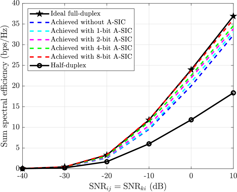
Figure 3: Sum spectral efficiency as a function of SNR for various scenarios. As the resolution of A-SIC improves, the sum spectral efficiency approaches that of ideal (interference-free) full-duplex.

V Conclusion

While there has been recent work to enable full-duplex mmWave systems via beamforming solutions, in this paper we suggest that such systems can be supplemented with A-SIC. Even with finite resolution A-SIC solutions, we demonstrate that significant gains can be had over mmWave full-duplex designs that rely solely on beamforming to mitigate the self-interference. Our design was validated in simulation which suggests that the sum spectral efficiency achieved during full-duplex operation can approach that of an ideal full-duplex system. To the best of our knowledge, this is the first work that combines beamforming with A-SIC to enable simultaneous transmission and reception in-band at mmWave.

References

- [1] J. G. Andrews, S. Buzzi, W. Choi, S. V. Hanly, A. Lozano, A. C. K. Soong, and J. C. Zhang, “What will 5G be?” IEEE Journal on Selected Areas in Communications, vol. 32, no. 6, pp. 1065–1082, Jun 2014.
- [2] I. P. Roberts and S. Vishwanath, “Beamforming cancellation design for millimeter-wave full-duplex,” in Proceedings of the 2019 IEEE Global Communications Conference: Signal Processing for Communications, Waikoloa, HI, USA, Dec. 2019.
- [3] K. Satyanarayana, et al., “Hybrid beamforming design for full-duplex millimeter wave communication,” IEEE Transactions on Vehicular Technology, vol. 68, no. 2, pp. 1394–1404, Feb. 2019.
- [4] B. Radunovic, D. Gunawardena, P. Key, A. Proutiere, N. Singh, V. Balan, and G. Dejean, “Rethinking indoor wireless mesh design: Low power, low frequency, full-duplex,” in Fifth IEEE Workshop on Wireless Mesh Networks. IEEE, 2010, pp. 1–6.
- [5] J. I. Choi, M. Jain, K. Srinivasan, P. Levis, and S. Katti, “Achieving single channel, full duplex wireless communication,” in Proceedings of the 16th annual international conference on mobile computing and networking. ACM, 2010, pp. 1–12.
- [6] M. Jain, J. I. Choi, T. Kim, D. Bharadia, S. Seth, K. Srinivasan, P. Levis, S. Katti, and P. Sinha, “Practical, real-time, full duplex wireless,” in Proceedings of the 17th annual international conference on mobile computing and networking. ACM, 2011, pp. 301–312.
- [7] D. Bharadia, E. McMilin, and S. Katti, “Full duplex radios,” in ACM SIGCOMM Computer Communication Review, vol. 43, no. 4. ACM, 2013, pp. 375–386.
- [8] I. P. Roberts, H. B. Jain, and S. Vishwanath, “Frequency-selective beamforming cancellation design for millimeter-wave full-duplex,” Oct. 2019, arXiv:1910.11983 [eess.SP].
- [9] R. W. Heath, N. Gonzalez-Prelcic, S. Rangan, W. Roh, and A. M. Sayeed, “An overview of signal processing techniques for millimeter wave MIMO systems,” IEEE Journal of Selected Topics in Signal Processing, vol. 10, no. 3, pp. 436–453, Apr. 2016.
- [10] J. S. Jiang and M. A. Ingram, “Spherical-wave model for short-range MIMO,” IEEE Transactions on Communications, vol. 53, no. 9, pp. 1534–1541, Sep. 2005.
- [11] R. W. Heath Jr. and A. Lozano, Foundations of MIMO Communication. Cambridge University Press, 2018.