Fixed smooth convolutional layer for avoiding checkerboard artifacts in CNNs

Abstract

In this paper, we propose a fixed convolutional layer with an order of smoothness not only for avoiding checkerboard artifacts in convolutional neural networks (CNNs) but also for enhancing the performance of CNNs, where the smoothness of its filter kernel can be controlled by a parameter. It is well-known that a number of CNNs generate checkerboard artifacts in both of two process: forward-propagation of upsampling layers and backward-propagation of strided convolutional layers. The proposed layer can perfectly prevent checkerboard artifacts caused by strided convolutional layers or upsampling layers including transposed convolutional layers. In an image-classification experiment with four CNNs: a simple CNN, VGG8, ResNet-18, and ResNet-101, applying the fixed layers to these CNNs is shown to improve the classification performance of all CNNs. In addition, the fixed layer are applied to generative adversarial networks (GANs), for the first time. From image-generation results, a smoother fixed convolutional layer is demonstrated to enable us to improve the quality of images generated with GANs.

Index Terms—  Checkerboard artifacts, Convolutional neural networks, Deep learning, Fixed convolutional layers, Generative adversarial networks

1 Introduction

Convolutional neural networks (CNNs) [1, 2], which are a kind of deep neural networks (DNNs), have attracted attention because of their outstanding performance and have widely been used in many fields: image processing, natural language processing, acoustic/speech processing, and more. In research fields of image-to-image translation problems, e.g., image super-resolution, it is well-known that forward-propagation of upsampling layers including transposed convolutional layers causes images to be distorted by checkerboard artifacts [3]. In addition, checkerboard artifacts are also caused by backward-propagation of downsampling layers including strided convolutional layers  [3]. CNN architectures usually have upsampling layers and/or have downsampling layers, such as VGG [4], ResNet [5], and U-Net [6], for increasing and/or reducing the spatial sampling rate of feature maps, respectively [7]. For this reason, checkerboard artifacts affect most commonly-used CNNs.

To overcome checkerboard artifacts caused by upsampling layers, a few research has been done to reduce the effects of checkerboard artifacts  [8, 9, 3, 10, 11, 12, 13]. In particular, Sugawara et al. [12, 13] gave us two approaches to perfectly prevent checkerboard artifacts by extending a condition for avoiding checkerboard artifacts in linear multirate systems  [14, 15, 16, 17]. However, the literature [12, 13] mainly focuses on checkerboard artifacts caused by upsampling layers, but there are few discussion about artifacts caused by downsampling layers. In addition, Sugawara et al. did not consider CNNs that have both upsampling and downsampling layers, such as generative adversarial networks (GANs)  [18]. Furthermore, in Sugawara’s method, only a zero-order hold kernel that has the lowest smoothness is used for avoiding checkerboard artifacts. Note that the smoothness of filter kernels is different from what has widely been considered for GANs, i.e., Lipschitz constraints  [19, 20, 21]. Hence, the effects of the smoothness on the performance of CNNs has never been discussed so far.

Because of such a situation, in this paper, we propose a novel fixed convolutional layer with an order of smoothness not only for perfectly avoiding checkerboard artifacts caused by upsampling and downsampling layers but also for enhancing the performance of CNNs. A filter kernel of the proposed layer is given by convolving a zero-order hold kernel multiple times. When using the proposed layer, we can control the smoothness of its filter kernel by changing the number of the convolution, referred to as the order of smoothness. In addition, we apply the proposed fixed layer to GANs for the first time,

We performed an image-classification experiment and an image-generation experiment in order to evaluate the effectiveness of the proposed fixed smooth convolutional layers. In the image-classification experiment with four CNNs: a simple CNN, VGG8, ResNet-18, and ResNet-101, applying the proposed layer is shown to improve the classification performance of all CNNs. From the image-generation results, a smoother fixed convolutional layer enables us not only to prevent checkerboard artifacts in GANs but also to improve the quality of images generated with GANs.

2 Preparation

In this section, we briefly summarize CNNs and checkerboard artifacts, where we only focus on 2-D convolutional layers for simplicity. We use notations shown in Table 1 throughout this paper.

Table 1: Notation

Symbol	Definition
$a$	A scalar
$\boldsymbol{a}$	A vector
$\boldsymbol{a}_{i}$	Element $i$ of vector $\boldsymbol{a}$, with indexing starting at $1$
$\mathrm{A}$	A matrix
$\mathrm{A}_{i,j}$	Element $i,j$ of matrix $\mathrm{A}$
$\mathrm{A}_{i,:}$	Row $i$ of matrix $\mathrm{A}$
$\mathrm{A}_{:,i}$	Column $i$ of matrix $\mathrm{A}$
$\boldsymbol{\mathrm{A}}$	A 3-D or higher-dimensional tensor
$\boldsymbol{\mathrm{A}}_{i,j,k}$	Element $i,j,k$ of 3-D tensor $\boldsymbol{\mathrm{A}}$
$\boldsymbol{\mathrm{A}}_{:,:,i}$	2-D slice of 3-D tensor $\boldsymbol{\mathrm{A}}$
$\boldsymbol{\mathrm{V}}$	A 3-D tensor with a size of channel $\times$ height $\times$ width, which denotes an input feature map for a layer.
$\boldsymbol{\mathrm{K}}$	A 4-D tensor with a size of output channel $\times$ input channel $\times$ height $\times$ width, which denotes a filter kernel (weights) of a convolutional layer.
$\boldsymbol{b}$	A vector with a size of output channel which denotes a bias of a convolutional layer.
$\boldsymbol{\mathrm{Z}}$	A 3-D tensor with a size of output channel $\times$ height $\times$ width, which denotes an output feature map of a layer.
$\mathrm{I}_{i}$	A single-channel image which is a 2-D slice $\boldsymbol{\mathrm{V}}_{i,:,:}$ of $\boldsymbol{\mathrm{V}}$.
$\mathrm{h}_{i,j}$	A 2-D filter which is a 2-D slice $\boldsymbol{\mathrm{K}}_{i,j,:,:}$ of filter kernel $\boldsymbol{\mathrm{K}}$.
$\mathcal{L}$	A loss function
$\mathbb{Z^{+}}$	The set of non-negative integers
$\mathrm{A}*\mathrm{B}$	The convolution on two matrices $\mathrm{A}$ and $\mathrm{B}$

2.1 Convolutional neural networks

A CNN is one of DNNs that has one or more convolutional layer(s). Calculation in a convolutional layer is given as

$$\boldsymbol{\mathrm{Z}}_{i,j,k}=\sum_{l,m,n}\boldsymbol{\mathrm{V}}_{l,j+m-1,k+n-1}\boldsymbol{\mathrm{K}}_{i,l,m,n}+\boldsymbol{b}_{i},$$ (1)

where $\boldsymbol{\mathrm{V}}$ denotes an input feature map, $\boldsymbol{\mathrm{K}}$ is a filter kernel, and $\boldsymbol{b}$ is a bias. Focusing on the $i$-th channel of an output feature map, the calculation of eq. (1) can be illustrated as a block-diagram by using a 2-D filter $\mathrm{h}_{i,j}=\boldsymbol{\mathrm{K}}_{i,j,:,:}$ and a single-channel image $\mathrm{I}_{j}$ = $\boldsymbol{\mathrm{V}}_{j,:,:}$, as shown in Fig. 1(1(a)).

(a) Convolution

(b) Strided convolution

(c) Transposed convolution

Fig. 1: Block diagram of convolutional layers

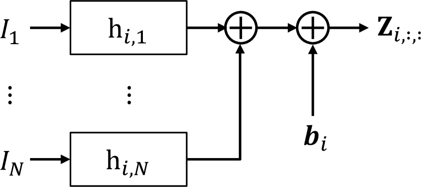
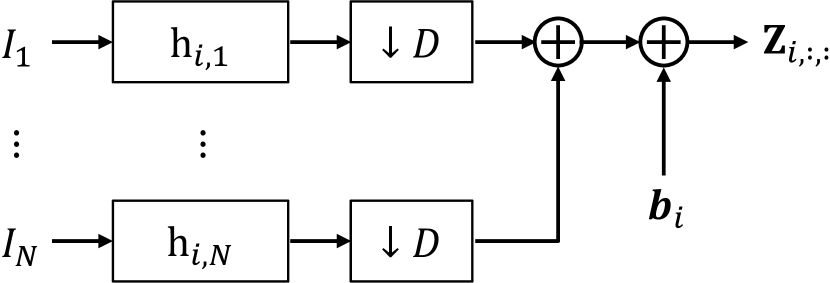
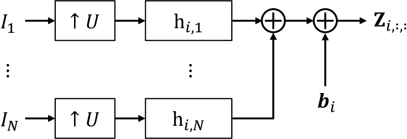
CNNs usually include upsampling layers and/or downsampling layers, to increase and/or reduce the spatial sampling rate (or the resolution) of feature maps, respectively. Typical downsampling layers are: strided convolutional layers, average pooling layers, and max pooing layers [7]. Here, average pooling layers and max pooling layers can be replaced with strided convolutional layers because:

• An average pooling layer is a particular kind of a strided convolutional layer.

• Replacing a max-pooling layer has little effect on the performance of CNNs  [22].

For these reasons, we focus on strided convolutional layers as downsampling layers. A strided convolutional layer is defined by the following equation:

$$\boldsymbol{\mathrm{Z}}_{i,j,k} =c(\boldsymbol{\mathrm{K}},\boldsymbol{\mathrm{V}},s)_{i,j,k}+\boldsymbol{b}_{i}$$

$$=\sum_{l,m,n}\boldsymbol{\mathrm{V}}_{l,(j-1)s+m,(k-1)s+n}\boldsymbol{\mathrm{K}}_{i,l,m,n}+\boldsymbol{b}_{i},$$ (2)

where $s\in\mathbb{Z^{+}}$ is a parameter called stride. Focusing on the $i$-th channel of an output feature map, the calculation of a strided convolutional layer corresponds to downsampling signals with a downsampling rate $D=s$ after convolving an input feature map $\mathrm{I}_{j}$ with a filter $\mathrm{h}_{i,j}$ [see Fig. 1(1(b))].

Upsampling layers includes a transposed convolutional layer, a sub-sampling layer [23], and a resize convolution layer [3]. In these layers, the most commonly-used transposed convolutional layer is given as

$$\boldsymbol{\mathrm{Z}}_{i,j,k} =t(\boldsymbol{\mathrm{K}},\boldsymbol{\mathrm{V}},s)_{i,j,k}+\boldsymbol{b}_{i}$$

$$=\sum_{\begin{subarray}{c}l,m\\ \mathrm{s.t.}\\ (l-1)s+m=j\end{subarray}}\sum_{\begin{subarray}{c}n,p\\ \mathrm{s.t.}\\ (n-1)s+p=k\end{subarray}}\sum_{q}\boldsymbol{\mathrm{V}}_{q,l,n}\boldsymbol{\mathrm{K}}_{q,i,m,p}+\boldsymbol{b}_{i}.$$ (3)

In contrast to a strided convolutional layer, the calculation for obtaining the $i$-th channel of an output feature map of a transposed convolutional layer corresponds to upsampling an input feature map $\mathrm{I}_{j}$ with an upsampling rate $U=s$ and then convolving the resulting feature map with a filter $\mathrm{h}_{i,j}$ [see Fig. 1(1(c))].

2.2 Upsampling and checkerboard artifacts

Checkerboard artifacts have been studied as a distortion caused by using upsamplers in linear multi-rate systems  [14, 15, 16, 17]. Figure 2(2(a)) shows a simple linear multi-rate system called linear interpolator that consists of an upsampler $\uparrow U$ with an upsampling rate $U$ and a linear time-invariant filter $\mathrm{h}$. To avoid checkerboard artifacts caused by the linear interpolator, it is necessary and sufficient that its filter $\mathrm{h}$ satisfies the following condition:

$$\mathrm{h}=\mathrm{h}_{0}*\mathrm{h}^{\prime},$$ (4)

where $\mathrm{h}_{0}$ and $\mathrm{h}^{\prime}$ are the zero-order hold kernel with a size of $U\times U$ and another linear time-invariant filter, respectively, and $*$ means the convolution on two matrices.

(a) Interpolator

(b) w/o checkerboard artifact

Fig. 2: Linear interpolator and avoiding checkerboard artifacts

A transposed convolutional layer has non-linear interpolators having a bias $b$, as in Fig. 3(3(a)). Sugawara et al. [12, 13] realized the perfect avoidance of checkerboard artifacts in non-linear interpolators by using the following two approaches:

1. Insert the zero-order hold kernel $\mathrm{h}_{0}$ after a filter $\mathrm{h}^{\prime}$ [see Fig. 3(3(b))]. This is equivalent to applying the condition in eq. (4) to $\mathrm{h}$.

2. Insert $\mathrm{h}_{0}$ after adding a bias $\boldsymbol{b}$, without any constraints on a filter $\mathrm{h}$ [Fig. 3(3(c))].

Note that Approaches 1 and 2 cannot be equivalently converted to each other.

(a) Interpolator w/ bias

(b) w/o checkerboard artifact (Approach 1)

(c) w/o checkerboard artifact (Approach 2)

Fig. 3: Non-linear interpolator with bias and avoiding checkerboard artifacts

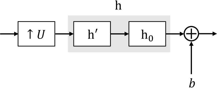
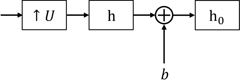
However, the literature [13] mainly focuses on checkerboard artifacts caused by upsampling layers, i.e., artifacts in the forward-propagation, but there are few discussion about artifacts caused by downsampling layers, i.e., artifacts in the backward-propagation. In addition, Sugawara et al. did not consider CNNs that have both upsampling and downsampling layers, such as GANs. Furthermore, in Sugawara’s method, a zero-order hold kernel that has the lowest smoothness is used for avoiding checkerboard artifacts, although we have a choice of the smoothness of filter kernels.

3 Proposed method

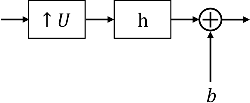
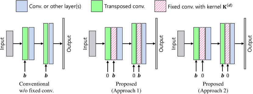
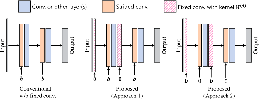
Figure 4 shows an usage of the fixed smooth convolutional layer that we propose. The proposed layer is a (depth-wise) convolutional layer and the smoothness of its filter kernel $\boldsymbol{\mathrm{K}}^{(d)}$ is controlled by a parameter $d$ called the order of smoothness. Similarly to Sugawara’s method in Section 2.2, there are two approaches to apply the proposed layer to a transposed convolutional layer or a strided convolutional layer, depending on the location of a bias $\boldsymbol{b}$.

(a) For transposed convolution

(b) For strided convolution

Fig. 4: Usage of proposed fixed convolution layer

3.1 Checkerboard artifacts in CNNs

Checkerboard artifacts in CNNs can be classified into artifacts in the forward-propagation and ones in the backward-propagation.

Checkerboard artifacts in the forward-propagation are caused by interpolators in transposed convolutional layers as shown in Fig. 1(1(c)), where the forward-propagation means a process calculating a new feature map $\boldsymbol{\mathrm{Z}}$ from an input feature map $\boldsymbol{\mathrm{V}}$ and passing the new feature map to the next layer. All filter kernels in transposed convolutional layers have to be trained to satisfy the condition in eq. (4), to prevent checkerboard artifacts. However, checkerboard artifacts cannot be prevented in practice because it is difficult to perfectly satisfy this condition by using an optimization algorithm. To resolve the issue, the use of fixed layers is required. Conventional CNNs with upsampling layers, which are mainly used for image super-resolution, distort an output feature map of each layer and an output image due to the artifacts. In addition, the artifacts affect training CNN models because the distorted output images are used for evaluating a loss function, for training the CNNs.

Checkerboard artifacts are also caused in the backward-propagation of a strided convolutional layer. The backward-propagation is a process calculating gradients of a loss function $\mathcal{L}$ with respect to parameters in a CNN, in order from the output layer to the input layer. In a strided convolutional layer, calculation of the gradient with respect to an input feature map $\boldsymbol{\mathrm{V}}$ is done by using transposed convolution $t(\cdot)$ as

$$\frac{\partial}{\partial\boldsymbol{\mathrm{V}}_{i,j,k}}\mathcal{L}(\boldsymbol{\mathrm{V}},\boldsymbol{\mathrm{K}})=t(\boldsymbol{\mathrm{K}},\boldsymbol{\mathrm{G}},s)_{i,j,k},$$ (5)

where a 3-D tensor $\boldsymbol{\mathrm{G}}$ of a gradient is given by an output-side layer and $\boldsymbol{\mathrm{K}}$ denotes a filter kernel that the strided convolutional layer has. For this reason, checkerboard artifacts appear in calculated gradients of CNNs with downsampling layers, which are generally used for image classification. Therefore, a filter kernels $\boldsymbol{\mathrm{K}}$ and a bias $\boldsymbol{b}$ in these CNNs will be affected by the checkerboard artifacts in gradients.

In addition, there are CNNs including both upsampling and downsampling layers, e.g., GANs [18] and the U-Net [6], which are generally used for image generation and image-to-image translation. These CNNs are affected by the checkerboard artifacts mentioned above.

3.2 Fixed smooth convolutional layer

A filter kernel $\boldsymbol{\mathrm{K}}^{(d)}$ of the proposed layer is obtained by convolving $\mathrm{h}_{0}$ multiple times, as

$$\boldsymbol{\mathrm{K}}^{(d)}_{i,i,:,:}=\begin{cases}\mathrm{h}_{0}&(d=0)\\ \boldsymbol{\mathrm{K}}^{(d-1)}_{i,i,:,:}*\mathrm{h}_{0}&(d>1)\end{cases},$$ (6)

where a parameter $d$, referred to as the order of smoothness, controls the smoothness of $\boldsymbol{\mathrm{K}}^{(d)}$. When the proposed layer is applied to an upsampling layer with an upsampling rate $U$, the kernel size for $\mathrm{h}_{0}$ is given as $U\times U$. In contrast, the kernel size is given as $D\times D$ when the proposed layer is applied to a downsampling layer with a downsampling rate $D$. By using a filter kernel $\boldsymbol{\mathrm{K}}^{(d)}$ and a trainable bias $\boldsymbol{b}$, an output feature map $\boldsymbol{\mathrm{Z}}$ of the proposed layer can be written as

$$\boldsymbol{\mathrm{Z}}_{i,j,k}=\sum_{m,n}\boldsymbol{\mathrm{V}}_{i,j+m-1,k+n-1}\boldsymbol{\mathrm{K}}^{(d)}_{i,i,m,n}+\boldsymbol{b}_{i}.$$ (7)

3.3 Avoiding checkerboard artifacts by the proposed layer

Checkerboard artifacts caused by a transposed convolutional layer can perfectly be prevented by using the proposed layer as follows [see also Fig. 4(4(a))]:

1. Fix a bias in a transposed convolutional layer as $0$, and insert the proposed layer having a trainable bias $\boldsymbol{b}$ after the transposed convolutional layer.

2. Insert the proposed layer having a bias which is fixed as 0 after a transposed convolutional layer having a trainable bias $\boldsymbol{b}$.

These approaches correspond to Approaches 1 and 2 in Section 2.2, respectively. The use of Approach 1 allows us to reduce computational costs since the redundancy of interpolators can be removed by the polyphase decomposition, but it will negate the effect of the bias $\boldsymbol{b}$ since the batch normalization (BN) is generally applied after each transposed convolutional layer. In contrast, under the use of Approach 2, the bias $\boldsymbol{b}$ is not affected by the BN but its computational costs cannot be reduced.

Checkerboard artifacts caused by a strided convolutional layer can also be prevented by inserting the proposed layer before the strided convolutional layer, in an opposite way to a transposed convolutional layer, because checkerboard artifacts in the strided convolutional layer occur in the backward-propagation [see 4(4(b))]. Similarly to the case of transposed convolutional layers, we can consider two approaches in terms of the location of a bias.

Both Approaches 1 and 2 for the proposed fixed layer can prevent checkerboard artifacts caused by both transposed convolutional layers and strided convolutional layers, under any order of smoothness $d$. In the next section, we will confirm that both Approaches 1 and 2 enhance the performance of CNNs and evaluate the quality of images generated by GANs under the use of the proposed layer having a high-order of smoothness.

4 Simulation

To evaluate the effectiveness of avoiding checkerboard artifacts by the proposed layer, we performed two simulations: image classification and image generation.

4.1 Image classification

We evaluated the classification accuracy of four CNNs with/without the proposed layer, in order to confirm the effectiveness of avoiding checkerboard artifacts in the backward-propagation. Here, we set all filter kernels of the proposed fixed layers as $\boldsymbol{\mathrm{K}}^{(0)}$. The following are the four CNNs used in this simulation: a simple CNN illustrated in Table 2, VGG8, ResNet-18, and ResNet-101, where ReLU in the table denotes the rectified linear unit activation function [24].

Table 2: Architecture of simple CNN. ch denotes number of output channels.

Layer	Stride $s$	Kernel size	ch
Conv. + BN + ReLU	2	$3\times 3$	64
Conv. + BN + ReLU	2	$3\times 3$	128
Conv. + BN + ReLU	2	$3\times 3$	256
Conv. + BN + ReLU	2	$3\times 3$	512
Conv. + BN + ReLU	1	$2\times 2$	10

In this simulation, we used the CIFER10 dataset [25] without any data augmentation for training and testing CNNs. Each CNN was trained with 300 epochs by using the Adam optimizer [26], where parameters in Adam were set as an initial learning rate of 0.1, $\beta_{1}=0.9$, and $\beta_{2}=0.999$, and we utilized an initial learning rate of 0.01 only for VGG8. In addition, each learning rate was multiplied by $1/10$ when the number of epoch reached 150 and 225.

Figure 5 shows the unit-step response of the backward-propagation of the second convolutional layer in the simple CNN with/without the proposed layers. From Fig. 5(5(a)), we can confirm that checkerboard artifacts appeared in calculated gradients when the simple CNN without the proposed layer was used. The artifacts were perfectly prevented by the proposed layers [see 5(5(a))].

(a) w/o fixed conv. layer

(b) with fixed conv. layer

Fig. 5: Unit step response of backward-propagation of second convolutional layer in simple CNN

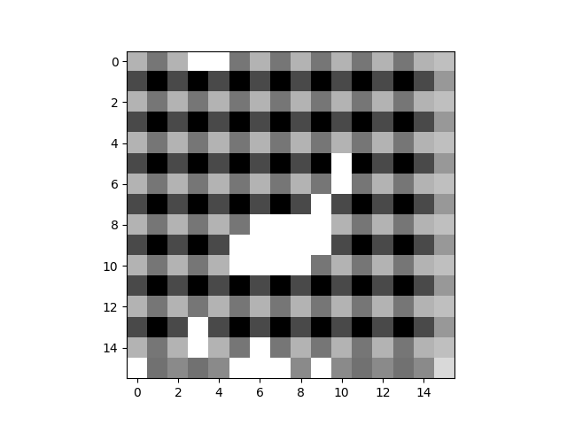
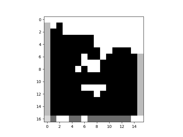
Table 3 illustrates the classification accuracy of the four CNNs. From Table 3, the proposed fixed layer improved the accuracy for the test set of all four CNNs. This improvement was confirmed in both Approaches 1 and 2 for avoiding checkerboard artifacts. The results illustrate that conventional CNNs for image classification were affected by checkerboard artifacts, and preventing the artifacts is effective for improving their performance.

Table 3: Image-classification accuracy for CIFER10 (train/test)

Network	Conv.	Prop. (Approach 1)	Prop. (Approach 2)
Simple CNN	0.999/0.585	0.999/0.645	0.976/0.671
VGG8	1.000/0.795	1.000/0.840	1.000/0.839
ResNet-18	1.000/0.812	1.000/0.862	1.000/0.862
ResNet-101	1.000/0.852	1.000/0.863	1.000/0.863

4.2 Image generation

In the simulation for image generation, we used generative adversarial networks (GANs)  [18, 27]. Basic GANs consists of two networks called “Generator” and “Discriminator,” respectively. Generally, a generator includes transposed convolutional layers and a discriminator includes strided convolutional layers. For this reason, checkerboard artifacts are generated in both the forward- and backward-propagation of GANs. To avoid the artifacts, we applied the proposed layers to GANs, where filter kernels of the proposed layer were $\boldsymbol{\mathrm{K}}^{(0)},\boldsymbol{\mathrm{K}}^{(1)}$, and $\boldsymbol{\mathrm{K}}^{(2)}$.

Tables 4 and 5 show the architectures of a generator and a discriminator used in the simulation, respectively, where Leaky ReLU [28] was utilized as activation functions in these networks.

Table 4: Generator architecture. ch denotes the number of output channels.

Layer	Stride $s$	Kernel size	ch
Trans. conv. + BN + Leaky ReLU	2	$4\times 4$	512
Trans. conv. + BN + Leaky ReLU	2	$4\times 4$	512
Trans. conv. + BN + Leaky ReLU	2	$4\times 4$	512
Trans. conv. + BN + Leaky ReLU	2	$4\times 4$	256
Trans. conv. + BN + Leaky ReLU	2	$4\times 4$	128
Trans. conv. + BN + Leaky ReLU	2	$4\times 4$	64
Conv. + Tanh	1	$3\times 3$	3

Table 5: Discriminator architecture. ch denotes the number of output channels.

Layer	Stride $s$	Kernel size	ch
Conv. + BN + Leaky ReLU	2	$4\times 4$	8
Conv. + BN + Leaky ReLU	2	$4\times 4$	32
Conv. + BN + Leaky ReLU	2	$4\times 4$	64
Conv. + BN + Leaky ReLU	2	$4\times 4$	64
Conv.	1	$4\times 4$	1

We trained GANs with 10 epochs by using 202,599 images in the CelebA [29] dataset in order to generate face images from 100-dimensional random vectors that follow the standard normal distribution, where the images were resized to $64\times 64$ pixels. The Adam optimizer [26] with an initial learning rate of 0.08, $\beta_{1}=0.5$, and $\beta_{2}=0.9$ was utilized for training both the generator and the discriminator.

Figure 6 illustrates an example of face images generated by using trained GANs. From the figure, checkerboard artifacts in generated images were suppressed by using the proposed layer although conventional GANs without the proposed layer caused the artifacts. Furthermore, the use of the proposed layers enables us to improve the quality of generated images. By comparing figures 6(6(b))，(6(c))， and (6(c)), it is confirmed that a sharp and clear image was generated when filter kernels $\boldsymbol{\mathrm{K}}^{(1)}$ and $\boldsymbol{\mathrm{K}}^{(2)}$ were used. From these results, the fixed convolutional layer having a smoother filter kernel provides GANs with a better performance.

(a) without fixed layers

(b) Proposed ($\boldsymbol{\mathrm{K}}^{(0)}$)

(c) Proposed ($\boldsymbol{\mathrm{K}}^{(1)}$)

(d) Proposed ($\boldsymbol{\mathrm{K}}^{(2)}$)

Fig. 6: Generated images by using GAN. Filter kernel $\boldsymbol{\mathrm{K}}^{(d)}$ of proposed fixed layer is controlled by order of smoothness $d$.

5 Conclusion

We proposed a novel fixed convolutional layer with an order of smoothness. The proposed layer can not only perfectly avoid checkerboard artifacts caused by transposed convolutional layers and strided convolutional layers, but also enhance the performance of CNNs including GANs. A filter kernel in the proposed layer is calculated by using a zero-order hold kernel and a parameter so-called the order of smoothness. From an image-classification experiment, it was confirmed that avoiding checkerboard artifacts by the proposed layer improved the classification performance of all four CNNs that we used in the experiment. In addition, an image-generation experiment demonstrated that a smoother fixed convolutional layer enables us to improve the quality of generated images by GANs while avoiding checkerboard artifacts, for the first time. In future work, we will further evaluate the proposed layer by more detailed simulations using other network architectures such as U-Net and discuss its effectiveness theoretically.

References

- [1] Y. LeCun, “Generalization and Network Design Strategies,” Department of Computer Science, University of Toronto, Tech. Rep., 1989.
- [2] A. Krizhevsky, I. Sutskever, and G. E. Hinton, “ImageNet Classification with Deep Convolutional Neural Networks,” in Proc. of International Conference on Neural Information Processing Systems, 2012, pp. 1097–1105.
- [3] A. Odena, V. Dumoulin, and C. Olah, “Deconvolution and Checkerboard Artifacts,” 2016. [Online]. Available: https://distill.pub/2016/deconv-checkerboard/
- [4] K. Simonyan and A. Zisserman, “Very Deep Convolutional Networks for Large-Scale Image Recognition,” arXiv preprint arXiv:1409.1556, Sep. 2014. [Online]. Available: http://arxiv.org/abs/1409.1556
- [5] K. He, X. Zhang, S. Ren, and J. Sun, “Deep Residual Learning for Image Recognition,” in Proc. of IEEE Conference on Computer Vision and Pattern Recognition, Jun. 2016, pp. 770–778.
- [6] O. Ronneberger, P.Fischer, and T. Brox, “U-Net: Convolutional Networks for Biomedical Image Segmentation,” in Medical Image Computing and Computer-Assisted Intervention, ser. LNCS, vol. 9351, Nov. 2015, pp. 234–241.
- [7] I. Goodfellow, Y. Bengio, and A. Courville, Deep learning. MIT Press, 2016.
- [8] J. Johnson, A. Alahi, and L. Fei-Fei, “Perceptual Losses for Real-Time Style Transfer and Super-Resolution,” in Proc. of European Conference on Computer Vision, 2016, pp. 694–711.
- [9] A. Aitken, C. Ledig, L. Theis, J. Caballero, Z. Wang, and W. Shi, “Checkerboard artifact free sub-pixel convolution: A note on sub-pixel convolution, resize convolution and convolution resize,” arXiv preprint arXiv:1707.02937, Jul. 2017. [Online]. Available: http://arxiv.org/abs/1707.02937
- [10] H. Gao, H. Yuan, Z. Wang, and S. Ji, “Pixel Deconvolutional Networks,” arXiv preprint arXiv:1705.06820, May 2017. [Online]. Available: http://arxiv.org/abs/1705.06820
- [11] Z. Wojna, V. Ferrari, S. Guadarrama, N. Silberman, L.-C. Chen, A. Fathi, and J. Uijlings, “The Devil is in the Decoder: Classification, Regression and GANs,” arXiv preprint arXiv:1707.05847, Jul. 2017. [Online]. Available: http://arxiv.org/abs/1707.05847
- [12] Y. Sugawara, S. Shiota, and H. Kiya, “Super-Resolution Using Convolutional Neural Networks Without Any Checkerboard Artifacts,” in Proc. of IEEE International Conference on Image Processing, Oct. 2018, pp. 66–70.
- [13] Y. Sugawara, S. Shiota, and H. Kiya, “Checkerboard artifacts free convolutional neural networks,” APSIPA Transactions on Signal and Information Processing, vol. 8, no. e9, Feb. 2019.
- [14] Y. Harada, S. Muramatsu, and H. Kiya, “Multidimensional Multirate Filter without Checkerboard Effects,” in Proc. of European Signal Processing Conference, 1998, pp. 1881–1884.
- [15] T. Tamura, M. Kato, T. Yoshida, and A. Nishihara, “Design of Checkerboard-Distortion-Free Multidimensional Multirate Filters,” IEICE Transactions on Fundamentals of Electronics, Communications and Computer Sciences, vol. E81-A, no. 8, pp. 1598–1606, Aug. 1998.
- [16] Y. Harada, S. Muramatsu, and H. Kiya, “Multidimensional Multirate Filter and Filter Bank without Checkerboard Effect,” IEICE Transactions on Fundamentals of Electronics, Communications and Computer Sciences, vol. E81-A, no. 8, pp. 1607–1615, Aug. 1998.
- [17] H. Iwai, M. Iwahashi, and H. Kiya, “Methods for Avoiding the Checkerboard Distortion Caused by Finite Word Length Error in Multirate System,” IEICE Transactions on Fundamentals of Electronics, Communications and Computer Sciences, vol. E93-A, no. 3, pp. 631–635, 2010.
- [18] I. Goodfellow, J. Pouget-Abadie, M. Mirza, B. Xu, D. Warde-Farley, S. Ozair, A. Courville, and Y. Bengio, “Generative Adversarial Nets,” in Advances in Neural Information Processing Systems, 2014, pp. 2672–2680.
- [19] M. Arjovsky, S. Chintala, and L. Bottou, “Wasserstein GAN,” arXiv preprint arXiv:1701.07875, Jan. 2017. [Online]. Available: http://arxiv.org/abs/1701.07875
- [20] I. Gulrajani, F. Ahmed, M. Arjovsky, V. Dumoulin, and A. Courville, “Improved Training of Wasserstein GANs,” arXiv preprint arXiv:1704.00028, Mar. 2017. [Online]. Available: http://arxiv.org/abs/1704.00028
- [21] T. Miyato, T. Kataoka, M. Koyama, and Y. Yoshida, “Spectral Normalization for Generative Adversarial Networks,” arXiv preprint arXiv:1802.05957, Feb. 2018. [Online]. Available: http://arxiv.org/abs/1802.05957
- [22] J. T. Springenberg, A. Dosovitskiy, T. Brox, and M. Riedmiller, “Striving for Simplicity: The All Convolutional Net,” arXiv preprint arXiv:1412.6806, Dec. 2014. [Online]. Available: http://arxiv.org/abs/1412.6806
- [23] W. Shi, J. Caballero, F. Huszar, J. Totz, A. P. Aitken, R. Bishop, D. Rueckert, and Z. Wang, “Real-Time Single Image and Video Super-Resolution Using an Efficient Sub-Pixel Convolutional Neural Network,” in Proc. of IEEE Conference on Computer Vision and Pattern Recognition, Jun. 2016, pp. 1874–1883.
- [24] X. Glorot, A. Bordes, and Y. Bengio, “Deep sparse rectifier neural networks,” in Proc. of the International Conference on Artificial Intelligence and Statistics, Apr. 2011, pp. 315–323.
- [25] A. Krizhevsky and G. E. Hinton, “Learning multiple layers of features from tiny images,” Master’s thesis, University of Toronto, 2009.
- [26] D. P. Kingma and J. Ba, “Adam: A Method for Stochastic Optimization,” arXiv preprint arXiv:1412.6980, Dec. 2014. [Online]. Available: http://arxiv.org/abs/1412.6980
- [27] A. Radford, L. Metz, and S. Chintala, “Unsupervised Representation Learning with Deep Convolutional Generative Adversarial Networks,” arXiv preprint arXiv:1511.06434, Nov. 2015. [Online]. Available: http://arxiv.org/abs/1511.06434
- [28] B. Xu, N. Wang, T. Chen, and M. Li, “Empirical Evaluation of Rectified Activations in Convolutional Network,” arXiv preprint arXiv:1505.00853, May 2015. [Online]. Available: http://arxiv.org/abs/1505.00853
- [29] Z. Liu, P. Luo, X. Wang, and X. Tang, “Deep Learning Face Attributes in the Wild,” in Proc. of International Conference on Computer Vision, Dec. 2015.