Turnpike Properties in Discrete-Time Mixed-Integer Optimal Control

Abstract

This note discusses properties of parametric discrete-time Mixed-Integer Optimal Control Problems (MIOCPs) as they often arise in mixed-integer NMPC. We argue that in want for a handle on similarity properties of parametric MIOCPs the classical turnpike notion from optimal control is helpful. We provide sufficient turnpike conditions based on a dissipativity notion of MIOCPs, and we show that the turnpike property allows specific and accurate guesses for the integer-valued controls. Moreover, we show how the turnpike property can be used to derive efficient node-weighted branch-and-bound schemes tailored to parametric MIOCPs. We draw upon numerical examples to illustrate our findings.

I Introduction

Recently, optimization-based control of dynamic systems has seen tremendous progress spanning from industrial applications of Non-linear Model Predictive Control (NMPC) [25, 12, 26] to efficient solution methods for Mixed-Integer Optimal Control Problems (MIOCPs) [2, 16, 27, 4, 17, 10]. By now, for considerably non-linear and non-convex cases implementation within the milli- to micro-second range can be achieved—provided the underlying continuous OCP can be approximated by a Non-Linear Programm (NLP), see e.g. [22]. These solution times are possible since the repeatedly solved optimization is parametric in the initial condition of the underlying dynamic system. In turn, this allows leveraging classical sensitivity properties of NLPs, see [8].

While transferring sensitivity concepts from OCPs and NLPs to MIOCPs and MINLPs is not straightforward, convincing cases have been made that also MIOCPs can be solved efficiently, e.g. [5, 27, 23] or [2, Chap. 7]. These works typically rely on efficient solutions to relaxed auxilliary problems, i.e. often they employ outer convexification. However, they do not explicitly exploit the parametric nature of the underlying MIOCP. Indeed only limited results on the analysis of parametric mixed-integer programs seem to be available. Multi-parametric MILPs, MIQPs and MINLPs are discussed in [11, 10, 20]. However, these results do not touch upon parametric MIOCPs.

In the present note we leverage dissipativity concepts to explicitly characterize helpful properties of parametric discrete-time MIOCPs. Specifically, we discuss cases of MIOCPs exhibiting the so-called turnpike property. Turnpikes occur in parametric OCPs where—for varying initial conditions and increasing horizon length—the time that optimal solutions spend outside of any $\varepsilon$-neighborhood of the optimal steady state is bounded independent of the actual horizon length. The turnpike notion was coined by [9] in the 1950s, and early observations of the phenomenon can be traced to works of John von Neumann in the 1930s/1940s [29]. There has been longstanding interest in turnpikes properties in the context of optimal control in economics [7]. Recently, there has been renewed interested in turnpikes for continuous OCPs [28, 15].

Herein, we argue that in want for a handle on similarity properties of parametric MIOCPs all is not lost, and that the turnpike notion enables such a characterization. Indeed, we advocate that in-depth investigation of turnpikes in parametric MIOCPs might open new avenues to tailored solution schemes for sequences of MIOCPs, e.g. arising in mixed-integer NMPC. Yet, to the best of the authors’ knowledge, there is no analysis of the turnpike phenomenon in MIOCPs available in the literature. To this end, we present a sufficient condition for turnpikes to arise which in turn is based on a dissipativity characterization of MIOCPs and we present a sufficient condition certifying dissipativity of linear-quadratic MIOCPS. Based on this, we sketch a tailored node-weighted branch-and-bound scheme which leverages the underlying turnpike for the sake of efficient solution. Numerical examples illustrate the benefits of the proposed scheme.

II Turnpikes in MIOCPs

We consider MIOCPs of the following form

$$\min_{x(\cdot),u(\cdot),v(\cdot)}\leavevmode\nobreak\ \sum\limits_{k=0}^{N-1}\ell(x(k),u(k),v(k))+V_{f}(x(N))$$ (1a)

$$\text{s.t. }\forall k \in\{0,\dots,N-1\},$$

$$x(k+1) =f(x(k),u(k),v(k)),\leavevmode\nobreak\ x(0)=x_{0}\in\mathbb{X}_{0}$$ (1b)

$$x(k) \in\mathbb{X}\subseteq\mathbb{R}^{n_{x}},\quad u(k)\in\mathbb{U}\subseteq\mathbb{R}^{n_{u}}$$ (1c)

$$v(k) \in\mathbb{V}\subseteq\mathbb{Z}^{n_{v}},$$ (1d)

where the stage cost $\ell:\mathbb{R}^{n_{x}}\times\mathbb{R}^{n_{u}}\times\mathbb{Z}^{n_{v}}\to\mathbb{R}$, the terminal cost $V_{f}:\mathbb{R}^{n_{x}}\times\mathbb{R}^{n_{u}}\times\mathbb{Z}^{n_{v}}\to\mathbb{R}$, and the dynamics $f:\mathbb{R}^{n_{x}}\times\mathbb{R}^{n_{u}}\times\mathbb{Z}^{n_{v}}\to\mathbb{R}^{n_{x}}$ are assumed to be Lipschitz continuous in $x$, $u$, and $v$. The constraint sets $\mathbb{X}$, $\mathbb{U}$ and $\mathbb{V}$ are assumed to be compact. The core challenge in the discrete-time OCP (1) is that the input $v$ is assumed to take only discrete values, cf. (1d).

Optimal solutions, provided they exist, are written as

$$z^{\star}(\cdot;x^{0})=\begin{bmatrix}x^{\star}(\cdot;x_{0})&u^{\star}(\cdot;x_{0})&v^{\star}(\cdot;x_{0})\end{bmatrix}^{\top}$$

denoting the optimal primal triplet. Whenever no confusion can arise, we suppress the dependence on the initial condition $x_{0}$. The stationary counterpart of (1) is the MINLP

$$\min_{\bar{x},\bar{u},\bar{v}} \leavevmode\nobreak\ \ell(\bar{x},\bar{u},\bar{v})$$ (2a)

s. t.

$$\bar{x} =f(\bar{x},\bar{u},\bar{v}),$$ (2b)

$$\bar{x} \in\mathbb{X}\subseteq\mathbb{R}^{n_{x}},\quad\bar{u}\in\mathbb{U}\subseteq\mathbb{R}^{n_{u}}$$ (2c)

$$\bar{v} \in\mathbb{V}\subseteq\mathbb{Z}^{n_{v}}.$$ (2d)

Simliar to before, the optimal solution is denoted by $\bar{z}^{\star}=\begin{bmatrix}\bar{x}^{\star}&\bar{u}^{\star}&\bar{v}^{\star}\end{bmatrix}^{\top}$. We are interested in studying the similarity properties of solutions to (1) for varying initial conditions $x_{0}\subset\mathbb{X}_{0}\subseteq\mathbb{X}$ and varying horizon lengths $N\in\mathbb{N}$. Put differently, we are interested in analyzing MIOCP (1) as a problem parametric in $x_{0}$ and $N\in\mathbb{N}$.

Illustrative Example

We consider a straight-forward modification of a simple problem presented in [14, 18] which reads

$$\min_{x(\cdot),u(\cdot),v(\cdot)} \sum\limits_{k=0}^{N-1}u(k)^{2}+{\textstyle\frac{1}{2}}v(k)^{2}$$

$$\text{s. t. }\forall k \in\{0,\dots,N-1\},$$ (3)

$$x(k+1) =2x(k)+u(k)+v(k)-1,\quad x(0)=x_{0}$$

$$\begin{bmatrix}x(k)\leavevmode\nobreak\ u(k)\leavevmode\nobreak\ v(k)\end{bmatrix}^{\top} \in[-2,2]\times[-3,3]\times\{-1,0,1\}.$$

Figure 1 shows the results for the horizon $N=30$ and several initial conditions $x_{0}$. Note that $z^{\star}(\cdot;x_{0})$ is close to its optimal steady state value $\bar{z}^{\star}=[1\leavevmode\nobreak\ 0\leavevmode\nobreak\ 0]^{\top}$ for a large part of the time horizon. This similarity of optimal solutions for different initial conditions is called turnpike phenomenon; a definition for MIOCPs will be given below.

Figure 1: Example plot of the optimal solutions for Problem (II) with $N=30$ and a variety of initial copnditions $x_{0}$.

Sufficient Conditions for Turnpikes in MIOCPs

First, we suggest a rigorous definition of the phenomenon:

Definition 1 (Mixed-integer turnpike property)

MIOCP (1) is said to have an input-state turnpike if for all $x_{0}\in\mathbb{X}_{0}$ and all $N\in\mathbb{N}$

$$\#\mathbb{Q}_{\varepsilon}\geq N-\frac{C}{\alpha(\varepsilon)}$$

holds, where

$$\mathbb{Q}_{\varepsilon}:=\{k\in\{0,\dots,N-1\}\hskip 2.84526pt|\hskip 2.84526pt||(z^{*}(k;x_{0}))-\bar{z}||\leq\varepsilon\},$$ (4)

$\#\mathbb{Q}_{\varepsilon}$ is the cardinality of $\mathbb{Q}_{\varepsilon}$, and $\alpha\in\mathcal{K}_{\infty}$.$\hfill\Box$

The above definition is a straight-forward extension of continuous concepts [18, 15]. Its basic meaning is that the amount of time an optimal triplet $z^{\star}(\cdot)$ spends inside of an $\varepsilon$-ball centered at $\bar{z}$ is at least $N-\frac{C}{\alpha(\varepsilon)}$, or alternatively, for all horizons the amount of time spent outside of the $\varepsilon$-ball is bounded independently of $N$ by $\frac{C}{\alpha(\varepsilon)}$. For the sake of brevity, we refer to $\bar{z}=\bar{z}^{\star}$ simply as the turnpike. We remark that the first part of the optimal solution approaching the turnpike is often called the entry arc, while the distinctive departure from the turnpike is called the leaving arc. Note that a leaving arc does not need to occur.

To the end of certifying turnpikes in mixed-integer problems, we recall and adapt an established dissipativity notion for OCPs to the mixed-integer setting.

Definition 2 (Strict dissipativity with respect to $\bar{z}$)

A system $x(k+1)=f(x(k),u(k),v(k))\doteq f(z(k))$ is said to be dissipative with respect to a steady-state tuple $\bar{z}\in\mathbb{X}\times\mathbb{U}\times\mathbb{V}$, if there exists a bounded function $\lambda:\mathbb{X}\rightarrow\mathbb{R}$ such that for all $z=\begin{bmatrix}x&u&v\end{bmatrix}^{\top}\in\mathbb{X}\times\mathbb{U}\times\mathbb{V}$

$$\lambda(f(z))-\lambda(x)\leq\ell(z)-\ell(\bar{z}),$$ (5a)

with $$\ell$$ from (1).

If, additionally, there exists $\alpha\in\mathcal{K}_{\infty}$ such that

$$\lambda(f(z))-\lambda(x)\leq-\alpha(\|z-\bar{z}\|)+\ell(z)-\ell(\bar{z}),$$ (5b)

then the system is said to be strictly dissipative with respect to $\bar{z}=\begin{bmatrix}\bar{x}&\bar{u}&\bar{v}\end{bmatrix}^{\top}$.

Moreover, if the above dissipativity notions holds solely along optimal solutions of (1) with $x_{0}\in\mathbb{X}_{0}$, then MIOCP (1) is said to be strictly dissipative with respect to $\bar{z}$. $\hfill\Box$

The following property follows directly from the above definition.

Lemma 1 (Optimality of $\bar{z}$)

Let MIOCP(1) be strictly dissipative with respect to $\bar{z}$ in the sense of Definition 2, then $\bar{z}=\bar{z}^{\star}$ is the unique globally optimal solution to (2).$\hfill\Box$

The next assumption helps to establish existence of turnpikes.

Assumption 1 (Exponential reachability of $\bar{x}^{\star}$)

For all $x_{0}\in\mathbb{X}_{0}$, there exist infinite-horizon admissible inputs $u_{\infty},v_{\infty}:\mathbb{N}\cap\infty\to\mathbb{U}\times\mathbb{V}$ and constants $c\geq 0,\rho\in[0,1)$ such that $\|x(k;x_{0},u_{\infty}(\cdot),v_{\infty}(\cdot))-\bar{x}^{\star}\|\leq c\rho^{k},$ i.e. the optimal steady state $\bar{x}^{\star}$ is exponentially reachable. $\hfill\Box$

Proposition 2 (Turnpikes in MIOCPs)

Let Assumption 1 hold and suppose that, for all $x_{0}\in\mathbb{X}_{0}$, the MIOCP (1) is strictly dissipative with respect to $\bar{z}^{\star}$. Then the MIOCP (1) has an input-state turnpike at $\bar{z}^{\star}=\bar{z}$. $\hfill\Box$

The proof follows the pattern of the ones presented in [14, 18] for continuous discrete-time OCPs and is thus omitted.

It is worth noticing that the turnpike property implies the following property of optimal solutions:

Proposition 3 (Integer controls exactly at turnpike)

For all $x_{0}\in\mathbb{X}_{0}$, let MIOCP (1) have an input-state turnpike at $\bar{z}^{\star}=\bar{z}$ in the sense of Definition 1. Then, for all $\varepsilon\in(0,1)$ and sufficiently large $N\in\mathbb{N}$, the optimal integer controls $v^{\star}(\cdot;x_{0})$ satisfy

$$\hskip 55.48277ptv^{\star}(k;x_{0})\equiv\bar{v}^{\star}\text{ for all }k\in\mathbb{Q}_{\varepsilon}.\hskip 58.32823pt\hfill\Box$$

Proof:

Recall that $\|z^{\star}(k;x_{0})-\bar{z}^{\star}\|\geq\|v^{\star}(k;x_{0})-\bar{v}^{\star}\|$, and note the fact that for the integer controls $\|v^{\star}(k;x_{0})-\bar{v}^{\star}\|<1\Leftrightarrow\|v^{\star}(k;x_{0})-\bar{v}^{\star}\|=0$. Combining both and taking the definition of $\mathbb{Q}_{\varepsilon}$ in (4) into account yields the assertion. ∎

It is fair to ask how the dissipativity property from Definition 2 can be numerically verified for MIOCPs. The next result provides a sufficient condition.

Theorem 4 (Dissipativity of linear-quadratic MIOCPs)

Consider MIOCP (1) and let the dynamics and the stage cost be given by

$$x^{+} =Ax+B_{1}u+B_{2}v,$$

$$\ell(x,u,v) =x^{\top}Qx+\begin{bmatrix}u\\ v\end{bmatrix}^{\top}R\begin{bmatrix}u\\ v\end{bmatrix}+q^{\top}x+r^{\top}\begin{bmatrix}u\\ v\end{bmatrix},$$

with potentially indefinite matrices $Q$ and $R$. If there exists a matrix $P\in\mathbb{R}^{n_{x}\times n_{x}}$ such that

$$Q+P-A^{\top}PA\succ 0,$$ (6)

then MIOCP (1) is strictly dissipative, and there exists $p\in\mathbb{R}^{n_{x}}$ such that $x^{\top}Px+p^{\top}x$ is a corresponding storage function.$\hfill\Box$

Proof:

The proof combines the available storage characterization of dissipativity with recent results from [19].

The available storage is given by

$$S^{a}_{\mathbb{V}}(x)= \sup_{z(\cdot),N}\leavevmode\nobreak\ \sum_{k=0}^{N}-\alpha(\|(z_{k})-\bar{z}\|)+\ell(z_{k})+\ell(\bar{z})$$

subject to

$$x(k+1) =Ax(k)+\begin{bmatrix}B_{1}&B_{2}\end{bmatrix}\begin{bmatrix}u(k)\\ v(k)\end{bmatrix},\leavevmode\nobreak\ x(0)=x$$

$$x(k) \in\mathbb{X},\leavevmode\nobreak\ u(k)\in\mathbb{U},\leavevmode\nobreak\ v(k)\in\mathbb{V},$$

whereby the subscript $\cdot_{\mathbb{V}}$ refers to the constraints on the discrete control input. Indeed the MICOP (1) is dissipative on $\mathbb{X}_{0}$ if $S^{a}_{\mathbb{V}}(x)<\infty$ for all $x\in\mathbb{X}_{0}$, cf. [30].

Step 1: Let $\operatorname{conv}\mathbb{V}$ be the convex hull of $\mathbb{V}$, which is compact if and only if $\mathbb{V}\subset\mathbb{Z}$ is compact. The inclusion $\mathbb{V}\subset\operatorname{conv}\mathbb{V}$ implies that

$$S^{a}_{\mathbb{V}}(x)\leq S^{a}_{\operatorname{conv}{\mathbb{V}}}(x),$$

i.e. dissipativity of the continuously relaxed OCP certifies dissipativity of the MIOCP.

Step 2: For the continuously relaxed problem it has been shown in [19, Lem. 4.1] that (6) is a necessary and sufficient condition for strict dissipativity with quadratic storage function on bounded subsets of $\mathbb{R}^{n_{x}}$. Combining both facts yields the assertion. ∎

Remark 1 (Turnpikes and parametric MIOCPs)

The above results highlight that turnpikes are to be understood as similarity properties of parametric MIOCPs. We remark that the Propositions 2 and 3 apply to non-convex and convex MIOCPs alike. They also allow for linear and nonlinear dynamics. Moreover, Theorem 4 addresses linear-quadratic problems, which however also do not need to be convex, i.e. indefinite matrices $Q,R$ are included. We remark that the solution $P$ to the Lyapunov equation (6) does not need to be positive definite. Moreover, notice that dissipativity of the MICOP does not depend on the specific choices of the linear weightings $q,r$ in the cost function. $\hfill\Box$

We proceed to sketch how these findings can be leveraged to design efficient solution strategies for MIOCPs.

III Branch and Bound with Node Weighting

Here we focus on an intuitive strategy for branch-and-bound algorithms that allows for exploiting a-priori knowledge of a turnpike. Specifically we suggest prioritizing exploration of nodes of the decision tree which are associated with the steady state optimal integer decisions at the turnpike (which is usually in the middle of the time horizon).

 

Algorithm 1: Branch and Bound with Node Weighting
 
Input: Guesses $\mathcal{V}_{0}=\{\mathbf{V}_{0,1},\dots,\mathbf{V}_{0,M}\}$ and corresponding weights $\mathcal{W}_{0}=\{w_{0,1},\dots,w_{0,M}\}$. Termination tolerance $\epsilon>0$. Default search strategy (depth-first, breadth-first, $\dots$) and corresponding weights $\mathcal{W}$.

Preparation: Set $U=\infty$, $L=-\infty$, $\mathcal{T}=\emptyset$. Re-index nodes $\mathcal{N}$ according to weights $\mathcal{W}_{0}$. Candidate node set $\mathcal{S}=\{0\}$.

While $\mathcal{S}\neq\emptyset$:

1. $\displaystyle\forall n\in\mathcal{S}$ 
   $\displaystyle\tilde{w}(n)=w(n)+\sum_{i=1}^{M}w_{0,i}\left(\operatorname{d}_{\mathbb{V}}(\mathbf{V}_{0,i})-\|\mathbf{V}_{0,i}-\mathbf{V}_{n}\|_{0}\right)$

2. $\displaystyle\tilde{n}=\underset{n\in\mathcal{S}}{\arg\max}\leavevmode\nobreak\ \tilde{w}(n)$ and $\mathcal{S}\leftarrow\mathcal{S}\setminus\{\tilde{n}\}$

3. Solve NLP($\mathbf{V}_{\tilde{n}}$) for $J^{\star}(\mathbf{V}_{\tilde{n}})$ and ${z}^{\star}(\mathbf{V}_{\tilde{n}})$ and $\mathcal{T}\leftarrow\mathcal{T}\cup\tilde{n}$

4. If ${z}^{\star}(\mathbf{V}_{\tilde{n}})$ is feasible in MIOCP (1) and $J^{\star}(\mathbf{V}_{\tilde{n}})<U$, then $U\leftarrow J^{\star}(\mathbf{V}_{\tilde{n}})$, proceed to Step 5.
   If $J^{\star}(\mathbf{V}_{\tilde{n}})>U$ proceed to Step 1.
   Else add the child nodes of $\tilde{n}$ to $\mathcal{S}$, proceed to Step 5.

5. $L\leftarrow\displaystyle\min_{n\in\mathcal{P}(\mathcal{S})}\{J^{\star}(\mathbf{V}_{n})\}$
   If $U-L\leq\epsilon$ terminate.
   Else proceed to Step 1.

 

To this end, let $\mathbf{V}\in\mathbb{R}^{n_{v}\times N}$ be a full or partial guess of the sequence of optimal integer decisions $v^{\star}(\cdot;x_{0})$ for Problem (1), and let $\mathbf{V}(k)$ denote its $k$-th column, which corresponds to the integer decisions for the $k^{th}$ time step.

Consider the following NLP relaxation of MIOCP (1)

$$\text{NLP}(\mathbf{V})=\left\{\text{\eqref{eq:MIOCP} with }\left\{\begin{array}[]{l l}v(k)=\mathbf{V}(k)&\text{if }\mathbf{V}(k)\in\mathbb{V}\\ v(k)\in\operatorname{conv}\mathbb{V}&\text{else}\end{array}\right.\right\},$$ (7)

i.e. $\eqref{eq:MIOCP_Z}$ is continuously relaxed. This relaxed problem takes $\mathbf{V}$ as a (partial or full) guess of the integer variables $v(0),\dots,v(N-1)$. The condition $\mathbf{V}(k)\not\in\mathbb{V}$ implicitly encodes the relaxation $\mathbf{V}(k)\in\operatorname{conv}\mathbb{V}$. We write $J^{\star}(\mathbf{V})$ and ${z}^{\star}(\mathbf{V})$ to denote the optimal performance bound, respectively, the (partially) relaxed solution triplet obtained from solving NLP($\mathbf{V}$). Let $\operatorname{d}_{\mathbb{V}}(\mathbf{V})$ denote the number of feasible integer components of $\mathbf{V}$, i..e. $\operatorname{d}_{\mathbb{V}}(\mathbf{V})=N\cdot n_{v}$ means for all $k\in\{0,\dots,N\}$ $\mathbf{V}(k)\in\mathbb{V}$, and $\operatorname{d}_{\mathbb{V}}(\mathbf{V})=0$ implies that all integer decisions are relaxed in (7).

Algorithm 1 lays out a straight-forward method for making use of $\mathbf{V}$ in the branch-and-bound decision tree that goes beyond warm-starting. For a decision tree consisting of nodes $\mathcal{N}$, let $\mathbf{V}_{n}$ denote the integer decision related to the node $n$ of the branch-and-bound tree, and let $\mathcal{P}(\mathcal{S})$ denote the parent nodes for a node set $\mathcal{S}\subseteq\mathcal{N}$. In Step 1 of Algorithm 1, the task is to determine which node should be explored first. To this end, the given guesses $\mathcal{V}_{0}$ and their corresponding chosen weights $\mathcal{W}_{0}$ are used. The number of different elements between the guess $\mathbf{V}_{0,i}$ and the integer vector at node $n$ of the branch-and-bound tree ,$\mathbf{V}_{n}$, is used to compute the weight update. Step 2 passes the node $\tilde{n}$ with the highest weighting and keeps track of explored nodes in the branch and bound tree, which is needed for computing the lower bound in Step 5. Step 3 fixes some integer variables according to the chosen node $\tilde{n}$, and the others take values from the convex relaxation of $\mathbb{V}$, cf. (7). Step 4 determines whether the upper bound should be updated, and if not whether child nodes of $n$ should be added to the list of candidate nodes. Finally, Step 5 checks whether the algorithm should terminate due to the upper and lower bounds being within the given tolerance $\epsilon$.

It is easy to see that Algorithm 1 inherits properties of standard branch-and-bound schemes, i.e. if the relaxed NLPs in Step 3 are solved to global optimality then a globally optimal solution to (1) will be found, as the worst case is full enumeration [21]. Observe that as such Algorithm 1 does not require any knowledge about a turnpike property. However, the turnpike of the underlying MIOCP can and should be encoded in ($\mathcal{V}_{0}$, $\mathcal{W}_{0}$). For example, this can be done by formulating guesses leveraging the insight of Proposition 3. In other words, the initial guesses ($\mathcal{V}_{0}$, $\mathcal{W}_{0}$) shall comprise high priority cases where $v(k)\equiv\bar{v}^{\star}$ holds.

Remark 2 (Alternative branching / weighting strategies)

We remark that one can imagine a generic branching strategy as following a specific node-weighting pattern. For example, a depth-first search weights lower nodes in the decision tree more highly, while a breadth-first search would weight the top nodes more than the bottom ones. However, in our prototpyical implementation, we observe that it is not advisable to explictly weight large swathes of the branch and bound tree nodes since computing the weighting and storing the resulting data can be computationally expensive. Rather, as illustrated in the example of the next section, just a few nodes should be weighted. The question of how many nodes to weight and how to construct weighting strategies for classes of problems that are not in the form of (1) are still open problems. $\hfill\Box$

IV Numerical Examples

To test the performance of Algorithm 1 we consider parametric convex linear-quadratic MIOCPs, which result in MIQPs and for which dissipativity can be checked via Theorem 4. The solutions are obtained using a prototypcial implementation of Algorithm 1 within MATLAB R2019a relying on CasADi v3.5.0 [1] and IPOPT to solve the QP subproblems. The implemented branch-and-bound algorithm starts with a depth-first branching strategy to obtain an upper bound and then seeks to improve the lower bound as quickly as possible. All numerical experiments were run on a 2.9GHz Intel Core i5-4460S CPU with 8GB of RAM.

Example 1

We consider the dynamics proposed in [3]:

$$x_{1}(k+1)=\begin{cases}\phantom{-}0.8x_{1}(k)+u(k),\quad\text{if }x_{1}(k)\geq 0,\\ -0.8x_{1}(k)+u(k),\quad\text{if }x_{1}(k)<0,\\ \end{cases}$$

with $\underline{x}\leq x_{1}(k)\leq\overline{x}$. This can be reformulated into a mixed-integer system of equations through the introduction of the continuous state variable $x_{2}$ and the discrete input $v$:

$$x_{1}(k+1) =0.8x_{2}(k)+u(k),$$ (8a)

$$2v(k)\underline{x} \leq x_{2}(k)+x_{1}(k)\leq 2v(k)\overline{x},$$ (8b)

$$2(v(k)-1)\overline{x} \leq x_{2}(k)-x_{1}(k)\leq 2(v(k)-1)\underline{x},$$ (8c)

$$(1-v(k))\underline{x} \leq x_{1}(k)\leq v(k)\overline{x},$$ (8d)

$$\underline{u} \leq u(k)\leq\overline{u},$$ (8e)

$$v(k) \in\{0,\,1\}.$$ (8f)

It is easy to verify that if $v(k)=0$ then $x_{2}(k)=-x_{1}(k)$ and $x_{1}(k)<0$, and if $v(k)=1$ then $x_{2}(k)=x_{1}(k)$ and $x_{1}(k)\geq 0$. The considered MIOCP reads:

$$\min_{z(\cdot)}\sum_{k=0}^{N-2}l^{\top}\left[\begin{smallmatrix}x_{1}(k)\\ x_{1}^{2}(k)\\ \phantom{{}_{1}}u(k)\\ u^{2}(k)\end{smallmatrix}\right]+l_{f}^{\top}\left[\begin{smallmatrix}x_{1}(N-1)\\ x_{1}^{2}(N-1)\\ \phantom{{}_{1}}u(N-1)\\ u^{2}(N-1)\end{smallmatrix}\right]$$ (9)

$$\text{subject to }\eqref{eq:mi_dyn}\text{ and }x_{1}(0)=x_{0},$$

with $l^{\top}=\begin{bmatrix}-10&100&10&100\end{bmatrix}$ and $l_{f}^{\top}=\begin{bmatrix}-1000&100&10&100\end{bmatrix}$.

All results presented use $\underline{x}=-1$, $\overline{x}=1$, $\underline{u}=0.5$, and $\overline{u}=0.5$. Algorithm 1 is provided a collection of complete discrete solution guesses and weights, as shown in Table I. Figure 2 depicts the optimal solution with $N=20$ and $x_{0}=1$. Note that one can clearly spot the turnpike at $\bar{z}^{\star}=\begin{bmatrix}-\frac{1}{9}&\frac{1}{9}&-0.2&0\end{bmatrix}$, which corresponds to solving (2) for this example. Shown in Table II are the aggregated results for each combination of $x_{1}(0)=\{\underline{x},\underline{x}+0.1,\dots,\overline{x}-0.1,\overline{x}\}$ for $N\in\{10,20\}$. These results compare Algorithm 1 without initial guesses (“std. B&B”) to Algorithm 1 leveraging the collection of solution vectors and weights from above (“node wthg”). The guesses and weights used are shown in Table I.

Figure 2: Opt. solutions for Example 1 with $N=20$ and $x_{0}=1$. Left: state trajectories $x_{1}$ (dashed blue) $x_{2}$ (solid red). Right: constrols $u$ (dashed blue) $v$ (solid red).

TABLE I: Guesses $\mathcal{V}_{0}$ and weights $\mathcal{W}_{0}$ for Example (9).

$\mathbf{V}_{0,i}$	$w_{0,i}$	$\mathbf{V}_{0,i}$	$w_{0,i}$
[1,1,0,$\dots$,0]	1	[1,1,1,0,$\dots$,0]	2
[1,1,1,0,$\dots$,0,1]	3	[1,1,1,0,$\dots$,0,1,1]	4
[1,1,1,0,$\dots$,0,1,1,1]	3	[1,1,1,0,$\dots$,0,1,1,1,1]	2

TABLE II: Results for Example 1 for 21 samples of $x_{0}$.

$T=20$	std. B&B	node wght
avg. # nodes	1125.15	925.24
median # nodes	1126	890
avg. runtime (s)	3000	466.01
median runtime	3000	274.83
best # nodes	1111	508
best runtime (s)	3000.12	90.63
avg. subopt.	423	0

$T=10$	std. B&B	node wght
avg. # nodes	503.43	147.71
median # nodes	515	102
avg. runtime (s)	739.87	149.95
median runtime	357.19	7.01
best # nodes	135	34
best runtime (s)	15.85	2.08
avg. subopt.	0	0

A termination limit of 3000 seconds is set for each test, however, the simple standard branch-and-bound algorithm often failed to terminate within this time for many of the larger problems, which is the cause of some suboptimality. As evidenced by the results in Table II, the proposed node weighting, which exploits the turnpike property of MIOCP (9), yields solutions much more quickly.

Example 2

As a second example we consider

$$\min_{z} \quad\sum_{k=0}^{N-1}\ell(z(k))$$

s. t. $$\forall k\in\{0,\dots,N-1\},$$ (10)

$$x(k+1) =Ex(k)+B_{1}u(k)+B_{2}v(k),\leavevmode\nobreak\ x(0)=x_{0}$$

$$z(k) \in\mathbb{R}^{n_{x}}\times\{0,\,1\}$$

with $E=\begin{bmatrix}0&I\\ 0&0\end{bmatrix}$m $I\in\mathbb{R}^{n_{x}-1\times n_{x}-1}$ is the identity matrix, $\ell(z)=10u+v(k)+100u^{2}+100x^{\top}x$, and $B_{1}=\begin{bmatrix}0&0&\dots&0&1\end{bmatrix}^{\top}$, $B_{2}=\begin{bmatrix}1&1&\dots&1&1\end{bmatrix}^{\top}$. The turnpike is at $\bar{z}^{\star}=0$.

Shown in Figure 3 is an example of the optimal solutions for $N=20$ and three state variables $n_{x}=3$. Observe that while Problem (9) exhibits a so-called leaving arc—i.e. the optimal solutions depart from the turnpike towards the end of the horizon—this is not the case in Problem (IV).

The intial guesses $\mathcal{V}_{0}$ are constructed as partial guesses of the integer controls corresponding to $\overline{v}^{\star}$ for $k\geq\hat{k}$ with $\hat{k}=\{2,\dots,6\}$. Each time Algorithm 1 is called only one of the guesses is passed ($\#\mathcal{V}_{0}=1$), its weight is set to $w_{0,1}=4\cdot\max_{w\in\mathcal{W}}w$. Shown in Table III are the aggregated results for each combination of $x_{0}=\begin{bmatrix}-0.9&-0.8&\dots&0.8&0.9\end{bmatrix}^{\top}+r$ for $N=10,20$ and $40$, where $r$ is a uniformly distributed random vector whose entries range between $-0.1$ and $0.1$. Overall we consider 19 different samples of $x_{0}$. Moreover, we consider the dimension of the state to be $n_{x}=30$. As in Example (9), “node wght” denotes the results from Algorithm 1 using this weighting, while “std. B&B” does not use any initial guesses. The results seen in Table III illustrate the dramatic benefit even a simply node weighting strategy can give. It can be seen that the standard branch-and-bound method is an order of magnitude slower in the smallest case, and this gap only increases as the length of the turnpike increases. Note that all algorithms converge to the optimal solution. Part of the reason for the quick convergence is that rearranging nodes in the setup of Algorithm 1 results in a decision tree with some infeasible or integer-feasible solutions at the first nodes that are explored. This prunes many of the subsequent nodes and greatly reduces the search space.

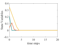
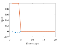
Figure 3: Optimal solution for Example 2 with $N=20$ and $\dim(x)=n_{x}=3$. Left: state trajectories. Right: controls $u$ (dashed blue) $v$ (solid red).

TABLE III: Results for Example 2 for 19 samples of $x_{0}\in\mathbb{R}^{30}$ and five different guesses $\mathcal{V}_{0}=\{\mathbf{V}_{0,1}\}$.

$T=10$	std.	node
$n_{x}=30$	B&B	wght
avg. # nodes	51.79	6.11
median # nodes	52	6
avg. runtime (s)	2.96	0.32
median time (s)	2.46	0.31
best # nodes	36	2
best runtime (s)	1.61	0.11

$T=40$	std.	node
$n_{x}=30$	B&B	wght
avg. # nodes	228.5	6.42
median # nodes	232	6
avg. runtime (s)	35.7	0.77
median time (s)	36.7	0.73
best # nodes	158	2
best runtime (s)	16.31	0.23

V Conclusions and Outlook

This note has taken first steps towards a turnpike theory for mixed-integer OCPs, thus paving the road for a better understanding of properties of parametric MIOCPs. Specifically, we have provided sufficient turnpike conditions based on a dissipativity notion of MIOCPs. We have also shown that the discrete controls will enter the turnpike exactly, while for the continuous controls this is not necessarily the case. For the special case of linear-quadratic MIOCPs we have presented an easy to check sufficient condition for dissipativity of MIOCPs on compact sets. Moreover, we have discussed how these insights can be easily leveraged to design node-weighted branch-and-bound schemes. While the present work appears to be the very first to discuss turnpikes in MIOCPs, at this stage our numerical results are an initial step relying on prototypical implementations. Future work will focus on several aspects including further exploitation of the turnpike phenomenon in branch-and-bound schemes for convex and non-convex MIOCPs.

Acknowledgement

The authors acknowledge helpful comments of Veit Hagenmeyer.

References

- [1] J.A.E. Andersson, J. Gillis, G. Horn, J.B. Rawlings, and M. Diehl. Casadi: a software framework for nonlinear optimization and optimal control. Mathematical Programming Computation, 11(1):1–36, 2019.
- [2] P. Belotti, C. Kirches, S. Leyffer, J. Linderoth, J. Luedtke, and A. Mahajan. Mixed-integer nonlinear optimization. Acta Numerica, 22:1–131, 2013.
- [3] A. Bemporad and M. Morari. Control of systems integrating logic, dynamics, and constraints. Automatica, 35(3):407–427, 1999.
- [4] A. Bemporad and V.V. Naik. A numerically robust mixed-integer quadratic programming solver for embedded hybrid model predictive control. IFAC-PapersOnLine, 51(20):412–417, 2018.
- [5] H.G. Bock, C. Kirches, A. Meyer, and A. Potschka. Numerical solution of optimal control problems with explicit and implicit switches. Optimization Methods and Software, 33(3):450–474, 2018.
- [6] P. Bonami, M. Kilinç, and J. Linderoth. Algorithms and software for convex mixed integer nonlinear programs. In Mixed Integer Nonlinear Programming, volume 154, pages 1–39. Springer, New York, 2012.
- [7] D.A. Carlson, A. Haurie, and A. Leizarowitz. Infinite Horizon Optimal Control: Deterministic and Stochastic Systems. Springer Verlag, 1991.
- [8] M. Diehl, I. Uslu, R. Findeisen, S. Schwarzkopf, F. Allgöwer, H.G. Bock, T. Bürner, E.D. Gilles, A. Kienle, J.P. Schlöder, and E. Stein. Real-time optimization for large scale processes: Nonlinear model predictive control of a high purity distillation column. In Online Optimization of Large Scale Systems, pages 363–383. Springer, 2001.
- [9] R. Dorfman, P.A. Samuelson, and R.M. Solow. Linear Programming and Economic Analysis. McGraw-Hill, New York, 1958.
- [10] V. Dua, N.A. Bozinis, and E.N. Pistikopoulos. A multiparametric programming approach for mixed-integer quadratic engineering problems. Computers & Chemical Engineering, 26(4-5):715–733, 2002.
- [11] V. Dua and E.N. Pistikopoulos. An algorithm for the solution of multiparametric mixed integer linear programming problems. Annals of operations research, 99(1-4):123–139, 2000.
- [12] S. Engell and I. Harjunkoski. Optimal operation: Scheduling, advanced control and their integration. Computers & Chemical Engineering, 2012.
- [13] T. Faulwasser and D. Bonvin. Exact turnpike properties and economic NMPC. European Journal of Control, 35:34–41, February 2017.
- [14] T. Faulwasser, L. Grüne, M.A. Müller, et al. Economic nonlinear model predictive control. Foundations and Trends® in Systems and Control, 5(1):1–98, 2018.
- [15] T. Faulwasser, M. Korda, C.N. Jones, and D. Bonvin. On turnpike and dissipativity properties of continuous-time optimal control problems. Automatica, 81:297–304, 2017.
- [16] M. Gerdts and S. Sager. Chapter 9: Mixed-integer DAE optimal control problems: Necessary conditions and bounds. In Control and Optimization with Differential-Algebraic Constraints, pages 189–212. SIAM, 2012.
- [17] T. Geyer. Generalized model predictive direct torque control: Long prediction horizons and minimization of switching losses. In Proceedings of the 48h IEEE Conference on Decision and Control (CDC) held jointly with 2009 28th Chinese Control Conference, pages 6799–6804. IEEE, 2009.
- [18] L. Grüne. Economic receding horizon control without terminal constraints. Automatica, 49(3):725–734, 2013.
- [19] L. Grüne and R. Guglielmi. Turnpike properties and strict dissipativity for discrete time linear quadratic optimal control problems. SIAM Journal on Control and Optimization, 56(2):1282–1302, 2018.
- [20] T. Gueddar and V. Dua. Approximate multi-parametric programming based B&B algorithm for MINLPs. Computers & Chemical Engineering, 42:288 – 297, 2012. European Symposium of Computer Aided Process Engineering - 21.
- [21] E. Hansen and G.W. Walster. Global optimization using interval analysis: revised and expanded, volume 264. CRC Press, 2003.
- [22] B. Houska, H.J. Ferreau, and M. Diehl. ACADO toolkit – an open-source framework for automatic control and dynamic optimization. Optimal Control Applications and Methods, 32(3):298–312, 2011.
- [23] C. Kirches, S. Sager, H.G. Bock, and J.P. Schlöder. Time-optimal control of automobile test drives with gear shifts. Optimal Control Applications and Methods, 31(2):137–153, 2010.
- [24] M. Lubin, E. Yamangil, R. Bent, and J.P. Vielma. Polyhedral approximation in mixed-integer convex optimization. Mathematical Programming, 2017.
- [25] S.J. Qin and T.A. Badgwell. An overview of nonlinear model predictive control applications. In F. Allgöwer and A. Zheng, editors, Nonlinear model predictive control, volume 26 of Progress in Systems and Control Theory, pages 369–392. Birkhäuser, 2000.
- [26] J.B. Rawlings, D.Q. Mayne, and M. Diehl. Model Predictive Control: Theory, Computation, and Design. Nob Hill Publishing, Madison, WI, 2017.
- [27] S. Sager, H.G. Bock, and M. Diehl. The integer approximation error in mixed-integer optimal control. Mathematical Programming, 133(1-2):1–23, 2012.
- [28] E. Trélat and E. Zuazua. The turnpike property in finite-dimensional nonlinear optimal control. Journal of Differential Equations, 258(1):81–114, 2015.
- [29] J. von Neumann. Über ein ökonomisches Gleichungssystem und eine Verallgemeinerung des Brouwerschen Fixpunktsatzes. In K. Menger, editor, Ergebnisse eines Mathematischen Seminars. 1938.
- [30] J.C. Willems. Dissipative dynamical systems part i: General theory. Archive for Rational Mechanics and Analysis, 45(5):321–351, 1972.