Compositional Abstraction-based Synthesis for Interconnected Systems: An approximate composition approach⋆
Abstract.
In this paper, we focus on mitigating the computational complexity in abstraction-based controller synthesis for interconnected control systems. To do so, we provide a compositional framework for the construction of abstractions for interconnected systems and a bottom-up controller synthesis scheme. In particular, we propose a notion of approximate composition which makes it possible to compute an abstraction of the global interconnected system from the abstractions (possibly of different types) of its components. Finally, by leveraging our notion of approximate composition, we propose a bottom-up approach for the synthesis of controllers enforcing decomposable safety specifications. The effectiveness of the proposed results is demonstrated using two case studies (viz., DC microgrid and traffic network) by comparing them with different abstraction and controller synthesis schemes.
1. Introduction
Control and verification of dynamical systems using discrete abstractions (a.k.a. symbolic models) and formal methods have been an ongoing research area in recent years (see [Tab09, BYG17] and the references therein). In such approaches, a discrete abstraction (i.e., a system with the finite number of states and inputs) is constructed from the original system. When the concrete and abstract systems are related by some relations such as simulation, alternating simulation or their approximate versions, the discrete controller synthesized for the abstraction can be refined into a hybrid controller for the original system. The use of discrete abstractions principally enables the use of techniques developed in the areas of supervisory control of discrete event systems [CL09] and algorithmic game theory [BJP+12]. The construction of such discrete abstractions is often based on a discretization of the state and input sets. Due to those sets discretization, symbolic control techniques suffer severely from the curse of dimensionality (i.e, the computational complexity for synthesizing abstractions and controllers grows exponentially with the state and input spaces dimension).
To tackle this problem, several compositional approaches were recently proposed. The authors in [TI08] proposed a compositional approach for finite-state abstractions of a network of control systems based on the notion of interconnection-compatible approximate bisimulation. The results in [PPD16] provide compositional construction of approximately bisimilar finite abstractions for networks of discrete-time control systems under some incremental stability property. In [MSSM18], the notion of (approximate) disturbance simulation was used for the compositional synthesis of continuous-time systems, where the states of the neighboring components were modeled as disturbance signals. In [ZA17], authors provide compositional abstraction using dissipativity approach. The authors in [DT15, KAS17, SGF18a, SGF18b, SGF20] use contract-based design and assume-guarantee reasoning to provide compositional construction of symbolic controllers.
In this paper, we provide a compositional abstraction-based controller synthesis framework for a composition of control systems. The main contributions of the work are divided into three parts. First, we introduce a notion of approximate composition, while the classical exact composition of components requires the inputs and outputs of neighboring components to be equal, we propose a notion of approximate composition allowing the distance between inputs and outputs of neighboring components to be bounded by a given parameter. The proposed notion enables the composition of control systems (possibly of different types) which allows for more flexibility in the design of the overall symbolic model because each component may be suitable for a particular type of abstraction. Second, with the help of the aforementioned notion, we provide results on the compositional construction of abstractions for interconnected systems. Indeed, given a collection of components, where each concrete component is related to its abstraction by an approximate (alternating) simulation relation, we show how the parameter of the composition of the abstractions needs to be chosen in order to ensure an approximate (alternating) simulation relation between the interconnection of concrete components and the interconnection of discrete ones. Third, we propose a bottom-up approach for symbolic controller synthesis for the composition of control systems and decomposable safety specifications . Finally, we demonstrate the applicability and effectiveness of the results using two case studies (viz., DC microgrid and traffic network) and compare them with different abstraction and controller synthesis schemes in the literature.
Related works: First attempts to compute compositional abstractions has been proposed for exact simulation relation [Fre05, KVdS10] and simulation maps [TPL04], for which the construction of abstraction exists for restricted class of systems. In [TI08], the first approach to provide compositionality result for approximate relationships was proposed using the notion of interconnection-compatible approximate bisimulation. Different approaches have then been proposed recently using small-gain (or relaxed small-gain) like conditions [RZ18, PPD16, SZ19] and dissipativity property [ZA17]. In [HAT17], a compositional construction of symbolic abstractions was proposed for the class of partially feedback linearizable systems, where the proposed approach relies on the use of a particular type of abstractions proposed in [ZPMT12].The authors in [KAZ18] present a compositional abstraction procedure for a discrete-time control system by abstracting the interconnection map between different components. The authors in [LP19] propose a compositional approach on the construction of bounded error over-approximations of continuous-time interconnected systems. However, those results are only available for cyclic (cascade and parallel) composition of two components. In [LP17] the authors propose a compositional bounded error framework for two interconnected hybrid systems. However, they are based on a notion of language inclusion, which differs from the results presented in this paper.
In parallel, other different approaches have been proposed for compositional controller synthesis. In [DT15], the authors propose a compositional approach to deal with persistency specifications using Lyapunov-like functions. The authors in [LFM+16] use reachability analysis to provide a compositional controller synthesis for discrete-time switched systems and persistency specifications. In [MGW17, MD18, MSSM18, SNO16, GSB20] different approaches were proposed for compositional controller synthesis for safety, and more general LTL specifications. All these approaches are based on assume-guarantee reasoning [SGF18c] and generally suffer from the underlying conservatism. In [PPB18], the authors propose a decentralized approach to the control of networks of incrementally stable systems, enforcing specifications expressed in terms of regular languages, while showing the completeness of their decentralized approach with respect to the centralized one.
In comparison with existing approaches in the literature, our framework presents the following advantages:
-
•
It allows the use of different types of abstractions for individual components such as continuous [GP09] or discrete-time abstractions based on state-space quantization [Tab09], partition [MGW15], covering [Rei11], or without any state-space discretization [ZTA17]. Indeed, given a composed system made of interconnected components, we can deal with the following scenarios:
-
–
The original composed system is continuous-time and the local abstractions are continuous-time.
-
–
The original composed system is discrete-time and the local abstractions are discrete-time.
-
–
The original composed system is continuous-time and the local abstractions are discrete-time. In this case, we need to have a uniform time-discretization parameter for all components, which is a common assumption in all the results in the symbolic control literature, except of [SGF20] where the authors are using continuous-time assume-guarantee contracts to deal with components with different sampling periods.
-
–
-
•
We do not need any particular structure of the components such as incremental stability or monotonicity. Moreover, we do not rely on the use of small-gain or dissipativity like conditions;
-
•
The proposed approach allows us to develop a bottom-up procedure for controller synthesis which helps to reduce the computational complexity while ensuring completeness with respect to the monolithic synthesis.
A preliminary version of this work has been presented in the conference [SJZG18]. The current paper extends the approach in three directions: First, the approach is generalized from cascade interconnections to any composition structure. Second, while in [SJZG18] we showed how to build a safety controller using a bottom-up approach, in this paper we show also the completeness of the proposed controller with respect to the monolithic one. Third, while in [SJZG18], we only presented a simple numerical example, here the theoretical framework is applied to more realistic case studies: DC microgids and road traffic networks.
2. Transition Systems and Behavioral Relations
Notations: The symbols , , and denote the set of positive integers, non-negative integers, and non-negative real numbers, respectively. Given sets and , we denote by an ordinary map from to , whereas denotes set valued map. For any , the map is a pseudometric if the following conditions hold: (i) implies ; (ii) ; (iii) . We identify a relation with the map defined by if and only if . We use notation to denote the infinity norm. The null vector of dimension is denoted by .
First, we introduce the notion of transition systems similar to the one provided in [Tab09].
Definition 2.1.
A transition system is a tuple , where is the set of states possibly infinite, is the set of initial states, is the set of external inputs possibly infinite, is the set of internal inputs possibly infinite, is the transition relation, is the set of outputs, and is the output map.
We denote as an alternative representation for a transition , where state is called a -successor (or simply successor) of state , for some input . Given , the set of enabled (admissible) inputs for is denoted by and defined as . The transition system is said to be:
-
•
pseudometric, if the input sets , and the output set are equipped with pseudometrics and , respectively.
-
•
finite (or symbolic), if sets , , and are finite.
-
•
deterministic, if there exists at most a -successor of , for any and .
In the sequel, we consider the approximate relationship for transition systems based on the notion of approximate (alternating) simulation relation to relate abstractions to concrete systems. We start by introducing the notion of approximate simulation relation adapted from [JDDBP09].
Definition 2.2.
Let and be two transition systems such that and are subsets of the same pseudometric space equipped with a pseudometric and respectively , , are subsets of the same pseudometric space respectively equipped with a pseudometric respectively . Let . A relation is said to be an -approximate simulation relation from to , if the following hold:
-
(i)
, such that ;
-
(ii)
, ;
-
(iii)
, , , with
and satisfying .
We denote the existence of an -approximate simulation relation from to by .
Note that when and is a metric, we recover the notion of approximate simulation relation introduced in [GP07] and when , it is similar to approximate simulation relation given in [Tab09].
Approximate simulation relations are generally used for verification problems. If the objective is to synthesize controllers, the notion of approximate alternating simulation relation introduced in [Tab09] is suitable. Interestingly, the notions of approximate simulation and approximate alternating simulation coincide in the case of deterministic transition systems.
Definition 2.3.
Let and be two transition systems such that and are subsets of the same pseudometric space equipped with a pseudometric and respectively , , are subsets of the same pseudometric space respectively equipped with a pseudometric respectively . Let . A relation is said to be an -approximate alternating simulation relation from to , if it satisfies:
-
(i)
, such that ;
-
(ii)
, ;
-
(iii)
, , with such that , satisfying .
We denote the existence of an -approximate alternating simulation relation from to by .
One can readily see that when we recover the classical notion of approximate alternating simulation relation as introduced in [Tab09], and when and is a metric, we recover the notion of approximate simulation relation introduced in [GP07] the approximate alternating simulation relation coincides with strong alternating simulation relation given in [BPDB18].
Remark 2.4.
Note that the definitions of approximate alternating simulation relations used in this paper are slightly different from the classical ones. Unlike classical definitions, the choice of inputs in our definitions is constrained by some distance property. However, these constraints over inputs are not restrictive and the proposed notions of -approximate alternating simulation relations are compatible for different abstraction techniques presented in the literature.
3. Networks of Transition Systems and Approximate Composition
Given a system made of interconnected components, the computation of a direct abstraction of the whole system is computationally expensive. For this reason, we rely here on the notion of approximate composition allowing us to construct a global abstraction of the system from the abstractions of its components. To analyze the necessity of approximate composition, let us start with the simplest interconnection structure, a cascade composition of two concrete components, where the output of the first system is an input to the second one. When going from concrete (infinite) to abstract (finite) components, the output of the first system and the input to the second system do not coincide any more, since abstractions generally involve quantization of variables. To mitigate this mismatch, we introduce a notion of approximate composition, by relaxing the notion of the exact composition and allowing the distance between the output to the first component and input to the second one to be bounded by some given precision.
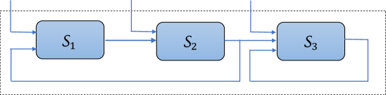
A network of systems consists of a collection of systems , a set of vertices and a binary connectivity relation where each vertex is labeled with the system . For , we define as the set of neighbouring components from which the incoming edges originate. An illustration of a network of interconnected components is given in Figure 1.
Definition 3.1.
Given a collection of transition systems , where such that for all , and are subsets of the same pseudometric space equipped with the following pseudometric:
| (3.1) |
Let . We say that is compatible for -approximate composition with respect to , if for each and for each , where the term can be formally defined as with , there exists such that . We denote -approximate composed system by and is given by the tuple , where:
-
•
; ;
-
•
; ;
-
•
;
-
•
for , and , if and only if for all , and for all , there exists with , and .
For the sake of simplicity of notations, we use instead of throughout the paper. Note that since all the internal inputs of a component are outputs of other components, the set of internal inputs of the composed system is simply the empty set. Hence, to improve readability, the composed system is defined without an internal input set. However, the same approach could be readily generalized to deal with a composed system with a given internal input set. If and is a metric, for all , we say that collection of systems is compatible for exact composition. Let us remark that, for the composed system, the set of enabled inputs will be defined with respect to the set . We equip the composed output space with the metric:
| (3.2) |
Similarly, we equip the composed input space with metric:
| (3.3) |
Let us remark that the parameter of the composition, i.e. , affects the conservativeness of the composed transition system. The following result shows that by increasing the parameter of the composition, the composed transition system allows for more nondeterminism in transitions and hence becomes more conservative. This result is straightforward and is stated without any proof.
Claim 3.2.
Consider a collection of systems and . If is compatible for -approximate composition with respect to , then it is also compatible for -approximate composition with respect to , for any such that i.e., , . Moreover, the relation is a -approximate simulation relation from to , where and .
4. Compositionality Results
In this section, we provide relations between interconnected systems based on the relations between their components. We first present the compositionality result for approximate alternating simulation relations.
Theorem 4.1.
Let and be two collection of transition systems with , and . Consider non-negative constants , , with and . Let the following conditions hold:
-
•
for all , with a relation ;
-
•
are compatible for -approximate composition with respect to , with ;
-
•
are compatible for -approximate composition with respect to , with .
Then the relation defined by
is an -approximate alternating simulation relation from to i.e., , where and .
Proof.
The first condition of Definition 2.3 is directly satisfied. Let with and . We have , where the first equality comes from the definition of the output map for approximate composition, the second equality follows from (3.2), and the inequality comes from condition (ii) of Definition 2.3.
Consider with and and any with . Let us prove the existence of with and such that for any , there exists satisfying . From the definition of relation , we have for all , , then from the third condition of Definition 2.3, we have for all , the existence of with and such that for any there exists such that .
Let us show that the input satisfies the requirement of the -approximate composition of the components . The condition implies that
Hence, from (iii) the - approximate composition with respect to of is well defined in the sense of Definition 3.1. Thus, condition (iii) in Definition 2.3 holds with satisfying , and one obtains . ∎
We then have the following compositionality result for approximate simulation relations.
Theorem 4.2.
Let and be two collection of transition systems with , and . Consider non-negative constants , , with and . Let the following conditions hold:
-
•
for all , with a relation ;
-
•
are compatible for -approximate composition with respect to , with ;
-
•
are compatible for -approximate composition with respect to , with .
Then the relation defined by
is an -approximate simulation relation from to i.e., , where and .
Proof.
The first condition of Definition 2.2 is directly satisfied. Let with and . We have where the first equality comes from the definition of the output map for approximate composition, the second equality follows from (3.2), and the inequality comes from the second condition of Definition 2.2.
Consider with and and any with . Consider the transition . This implies that for all , and for all , there exists with , and . Let us prove the existence of an input such that and a transition such that .
From the definition of the relation , we have for all , , and , then from the third condition of the Definition 2.2, there exists with and and there exists such that .
Let us show that the input satisfies the requirement of the -approximate composition of the components . The condition implies that
Hence, the - approximate composition with respect to of is well defined in the sense of Definition 3.1. Thus, condition (iii) in Definition 2.2 holds with satisfying and , and one obtains . ∎
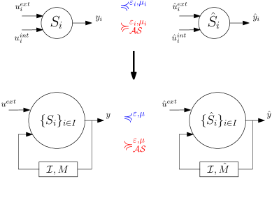
Intuitively, the results of the previous theorems can be interpreted as follows: the result in Theorem 4.2 can be used for compositional verification. Given a collection of systems , if each component approximately satisfies a specification (), then the composed system approximately satisfies a composed specification (). Note that for constructing controllers, the results of Theorem 4.1 is more suitable. Given a collection of components , for , let an abstraction for (), then the composed system is an abstraction of the system (). Figure 2 illustrates these results.
Remark 4.3.
In symbolic control literature, different approaches have been presented to compute infinite abstractions for different classes of systems including linear systems [BYG17, GP09], monotone or mixed-monotone systems [CA15, MGW15], time-delay systems [PPDBT10], switched systems [GPT09], incrementally stable or stabilizable systems [PGT08], incrementally stable stochastic switched systems [ZTA17] and incrementally stable time-delayed stochastic control systems [PPDBT10, JZ20]. Let us point out that the proposed compositional framework in this paper is suitable for different types of infinite abstractions which allows for modularity and flexibility in the construction of the symbolic models.
5. Bottom-up safety controller synthesis
In the previous section, we have shown how to derive approximate (alternating) simulation relations between the concrete and abstract models of the whole system from those of the components, which can mainly be used for the construction of compositional abstractions. Based on those results, in this section, we go one step further and show how the proposed compositionality results make it possible to provide a bottom-up approach for the synthesis of controllers enforcing decomposable safety specifications.
5.1. Controlled systems
Consider a system and a memoryless controller such that for all , . Let be the domain of controller defined by . We define a controlled transition system by a tuple , where:
-
•
is the set of states;
-
•
is the set of initial states;
-
•
is the set of external inputs;
-
•
is the set of internal inputs;
-
•
is the set of outputs;
-
•
is the output map;
-
•
a transition relation: if and only if and .
We first introduce the following auxiliary lemma relating the system and the controlled system .
Lemma 5.1.
Given the systems and defined above, we have that .
Proof.
Define the relation . We have that , hence the first condition of Definition 2.3 is satisfied. Let . We have that which shows condition (ii) of Definition 2.3. Now consider and any . We choose and with and . Then for all we have . Since , we have the existence of satisfying . This implies , which concludes the proof. ∎
5.2. Safety controller
Definition 5.2.
A safety controller for the transition system and the safe set satisfies:
-
(i)
;
-
(ii)
and , .
There are in general several controllers that solve the safety problem. A suitable solution is a controller that enables as many actions as possible. Such controller is referred to as a maximal safety controller, in the sense that for any other safety controller and for all , we have . In order to define carefully the maximal safety controller, we introduce the concept of a controlled invariant set.
Definition 5.3.
Consider a transition system and a safe set . A subset is said to be a controlled invariant if for all there exists such that .
It was shown in [Tab09] that there exists a maximal controlled invariant which is the union of all controlled invariants. The maximal safety controller can be defined as follows:
-
•
for all , ;
-
•
for all , .
Let us remark that for any safety controller we have that , while for the maximal safety controller , we have .
5.3. Bottom-up synthesis of controllers
The size of transition systems is crucial for computational efficiency of discrete safety controller synthesis algorithms. As the size of transition systems grows, the classical safety synthesis suffers from the curse of dimensionality. In this subsection, we show how to synthesize safety controllers for interconnected systems using a bottom-up approach. Consider a global system made of interconnected components , , and a global decomposable safety specification . We start by synthesizing a local safety controller for each component and safety specification , compose the local controlled components (by computing ), and then synthesize a global safety controller for against the safety specification . We first give an example illustrating the idea of bottom-up safety synthesis.
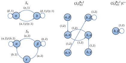
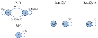
Example 5.4.
Consider the transition systems and as shown in Figure 4, where is the identity map. Let the interconnection relation be . Since and , the components and are compatible for exact composition with respect to . Let be the composed system. Let the global safety specification for the system define by , where and . The classical safety approach directly synthesize a maximal safety controller for the system . An illustration of the controlled system is given in Figure 4. In the proposed bottom-up approach, see Figure 4, we first start by synthesizing a local controller for the component against the safety specification to obtain . We then compose the local controlled components by computing . Finally we synthesize a global safety controller for the system against the safety specification . In the classical safety synthesis, we need to compute the safety controller for the system , which is made of states and transitions. In the proposed bottom-up synthesis, we need to apply the global safety synthesis for the reduced composed system which is made of states and transition111Let us mention that computational complexity to compute the local controllers for components is imperceptible with comparison to the safety synthesis on the global reduced composed system .. Hence, one can notice in this toy example the benefits of the proposed synthesis while ensuring completeness with respect to the classical safety synthesis ().
We start by providing the following auxiliary lemma showing how the maximal safety controller for the composed system is related to the maximal controllers synthesized for the components , .
Lemma 5.5.
Let be a collection of transition systems compatible for -approximate composition, with . Let be the composed system. Let be a safety specification for the composed system and let us assume the following:
-
•
, is the maximal safety controller for enforcing the specification ;
-
•
is the maximal controller for enforcing the safety specification .
If and for some and some , then we have .
Proof.
For , let us define the controller as follows: if and only if there exists and there exists such that and . Let us prove that is a safety controller for and safety specification .
Let , then by construction of we have the existence of such that . Hence, and , then condition (i) of Definition 5.2 is satisfied. Now let and . We have the existence of and such that and . Since is the maximal safety controller for the system and safety specification , we have that for all , . Hence, for , for all where is such that . Then, is a safety controller for the component and safety specification .
Now let . Then from construction of , for all , and for all such that , we get , where the last inclusion follows from the maximality of the controller for the component and specification , which concludes the proof. ∎
Next, we provide theorem showing the completeness of the proposed bottom-up controller synthesis procedure with respect to the maximal monolithic safety controller .
Theorem 5.6.
Let be a collection of transition systems compatible for -approximate composition, with . Let be the composed system. Let be a safety specification for the composed system and let us assume the following:
-
•
, is the maximal safety controller for enforcing the specification ;
-
•
is the maximal controller for enforcing the safety specification ;
-
•
is the maximal controller for enforcing the safety specification .
Then, for all , .
Proof.
From Lemma 5.1, we have for all , , then it follows from Theorem 4.1 that . Since is the maximal safety controller for and safety specification and from definition of the alternating simulation relation [Tab09], we have that is a safety controller for the system and specification . Then from maximality of , we have that for all .
To prove the second inclusion, let us first show that , with , and . Let the relation defined by
From Lemma 5.5 we have that , hence, and the first condition of Definition 2.3 is satisfied. Let , we have that , hence, and condition (ii) of Definition 2.3 is satisfied. Now, let and . Then and . We have from Lemma 5.5 that for all , for any satisfying . Then, by construction of the transition systems and , we have for all , . Hence there exists such that . Then, and condition (iii) of Definition 2.3 is satisfied.
Since is the maximal safety controller for and safety specification and from the definition of the alternating simulation relation [Tab09], we have that is a safety controller for the system and specification . Then from maximality of , we have that for all . Then for all , . ∎
In order to clarify the link between the results of Sections 4 and 5, the following remark is in order.
Remark 5.7.
Given a system made of interconnected components , , we have the following scenarios:
-
•
If we have a decomposable safety specification, , we start by constructing a local abstraction for each component , synthesize a local safety controller for each local abstraction and safety specification , compose the local controlled abstractions (by computing ), using the result of Theorems 4.1 and 4.2, and then synthesize a global safety controller for against the safety specification , while ensuring in view of Theorem 5.6 the completeness of the proposed bottom-up synthesis approach with respect to the monolithic abstraction-based synthesis (cf. traffic flow example in Subsection 6.2).
-
•
If we have any other type of specification , such as reachability, stability, non-decomposable safety specification or more general LTL formula, we start by constructing a local abstraction for each component , use the result of Theorems 4.1 and 4.2 to compute a global abstraction from the local ones, and then synthesize the controller monolithically (cf. DC microgrids example in Subsection 6.1).
6. Numerical examples
In this section, we demonstrate the effectiveness of the proposed approach on two control problems: a DC microgrid and a road traffic control problem. The objective of the first example is to illustrate the speed-up that can be attained using the compositional abstraction framework proposed in Section 4. In the second example, we show how the proposed framework can be applied to a more complex example, on which different abstraction techniques are used for different components to show the efficacy of proposed results in Section 4. Additionally, we will also show the benefits of the bottom-up safety synthesis approach proposed in Section 5. In the following, the numerical implementations have been done in MATLAB and a computer with processor 2.7 GHz Intel Core i5, Memory 8 GB 1867 MHz DDR3.
6.1. DC microgrids
Direct-current (DC) microgrids have been recognized as a promising choice for the redesign of distribution systems, which are undergoing relevant changes due to the increased penetration of photovoltaic modules, batteries and DC loads. A microgrid is an electrical network gathering a combination of generation units, loads and energy storage elements. Here, we use the DC microgrid model proposed in [ZSGF19b].
6.1.1. Model description and control objective
We represent a microgrid as a directed graph , where: is the set of nodes, with cardinality ; is the set of edges, with cardinality and is the incidence matrix capturing the graph topology. The edges correspond to the transmission lines, while the nodes correspond to the buses where the power units are interfaced. The weighted interconnection topology is equivalently captured by the Laplacian matrix , with , where denotes the conductance associated to the edge . We further define as the subset of nodes associated to controllable power units (sources), i.e. the generation and energy storage units, with cardinality , and as the subset of nodes associated to non-controllable power units (loads), with cardinality . The interconnected dynamics of the voltage buses are:
| (6.1) |
where denotes the collection of (positive) bus voltages, denotes the collection of input currents and , are matrices denoting the bus capacitances and conductances. Input currents are given by:
| (6.2) |
with: control input , where ; , where , if and otherwise; and is a bounded time-varying demand . By replacing (6.2) into (6.1), the overall system can be rewritten in compact form as
| (6.3) |
with state vector ; control input , where ; disturbance input ; and where denotes the element-wise division of matrices.
The safe set is given by and means that the voltage of the system need to be kept sufficiently near to the nominal value up to a given precision .
6.1.2. Abstraction and controller synthesis
We consider a five-terminal DC microgrid as the one depicted in Figure 5. We assume that two units, namely Units and , are equipped with a primary control layer, while the remaining three units, Units , , and correspond to loads with demand varying steadily around a constant power reference. The latter can be thus interpreted as constant power loads affected by noise.

The considered bus parameters are , , , and the network parameters are , , , , , , .
The system is supposed to operate within a region with grid nominal voltage and . We use the symbolic approach presented in [MGW15], while exploiting the monotonicity property of the DC grid [ZSGF19a], we select sampling period for the abstractions milliseconds, which corresponds to the clock of the controller to be designed. Discretization parameters are and denoting the number of discrete states and inputs, respectively, for each dimension.
We consider two scenarios. In the first case, we assume that Unit is disconnected from the grid and the grid is made of units . We compute local abstraction for each Unit , , each abstraction is related to the original system , , by an -approximate alternating simulation relation, with and . We then compose the local abstractions in order to compute the global abstraction using an -approximate composition, with . Hence, in view of Theorem 4.1, we have that 222Given the safety specification for the original system and since the original system is related to the compositional abstraction by an approximate alternating simulation relation, the abstract specification is a deflated version of the original one, and is given by ., where and .
The computation time of the abstractions of the four components are given by seconds, seconds, seconds and seconds, respectively, and the composition of the global abstraction from local ones using an approximate composition takes seconds. This resulted in seconds to compute an abstraction compositionally. Constructing an abstraction for the full model monolithically, using the same discretization parameters, took seconds. Hence, the proposed compositional approach was three times faster in this scenario.
In the second scenario, Unit is connected to the grid, we use the same numerical parameters as in the first scenario. In this case, the computation time of the abstraction of the five components are given by seconds, seconds, seconds, seconds, and seconds, respectively, and the composition of the global abstraction from local ones using an approximate composition takes minutes. Let us mention that with comparison to the previous scenario (where only Units 1 to 4 are considered), only the computation time of Unit 2 is modified, since it is the only Unit connected to Unit 5 (see Figure 5). Using the same numerical values, the direct computation of the monolithic abstraction takes hours, which shows the practical speedups that can be attained using the compositional approach. For the same example, the number of controllable states for the monolithic and compositional schemes is the same and is given by 3125. The size of resulting controllers (number of transitions) for the monolithic and compositional schemes is given by 18252 and 11040, respectively. Hence, it can be seen that the speed-up of the computation of the abstraction using the proposed compositional approach here results in losing the abstraction precision in comparison with the monolithic one, which is observed from the size of the obtained controllers.
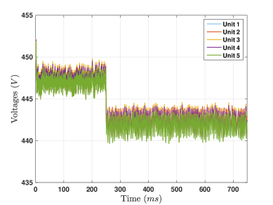
We then synthesize a safety controller for the computed abstraction. The synthesis of the symbolic controller takes seconds. To validate our controller, we assume that the load power demands for Unit 1, Unit 4 and Unit 5 are as follows. Unit 1 is demanding from to milliseconds, immediately after stepping up to . Unit 4 on the other hand is supposed to be characterized by a demand of from to milliseconds, then a constant demand of from milliseconds to milliseconds. Finally, Unit 5 is characterized by a demand of from to milliseconds, then a constant demand of from milliseconds to milliseconds. All demands are affected by small noise. Source power injections are positive and both limited at . The controller is implemented via a microprocessor of clock period milliseconds. Voltage responses for different units are illustrated in Figure 6. As expected, the controller guarantees that voltages are kept sufficiently near the nominal value.
6.2. Traffic flow model
For the second example, we consider a popular macroscopic traffic flow model used for the analysis of highway traffic behavior is the cell transmission model (CTM) introduced in [Dag94].
6.2.1. Model description and control objective
Here we consider the traffic flow model as shown schematically in Figure 7 and described by
| (6.4) |
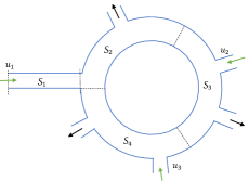
where the state , , represents the density of traffic in section of road given in vehicles per section, is the length of road, is the flow speed, hours is the discrete time interval, and is the ratio representing the percentage of vehicles leaving the section of road. The control inputs , where 0 represents red signal and 1 represents green signal in the traffic model. We consider the compact state-space . The control objective is to synthesize controller to keep states in a safe region given by .
6.2.2. Abstraction and controller synthesis
We consider four subsystems , , corresponding to four sections in traffic network model. To demonstrate the effectiveness of the proposed result on bottom-up safety controller synthesis, we compare results obtained using monolithic safety synthesis and bottom-up safety synthesis on compositional abstractions. For constructing abstractions, we construct an -approximate bisimilar abstraction of called using state-space discretization-free abstraction techniques as discussed in [LCGG13, ZTA17] using tool QUEST [JZ17]. For construction of , with precision and , we consider , length of input sequence , and source state (for description and computation of parameters and , see [LCGG13] and [ZTA17]). The abstractions , , are computed by utilizing partitions of the state-space as shown in [MGW15, RWR17], each abstraction is related to the original component by an -approximate alternating simulation relation, with and . Note that since the subsystem is incrementally input-state stable and do not have any internal input, the input set of the component is much smaller compared to other components. In such a scenario, state-space discretization-free abstractions are efficient compared to state-space discretization based abstractions (see Section 4.D in [LCGG13] and Section 5.4 in [ZTA17] for detailed discussion).
Monolithic and proposed bottom-up approaches to safety synthesis are then compared. In the first one, we compute the global compositional abstraction by composing local abstractions with a composition parameter . We then monolithically synthesize a safety controller for the global abstraction with the safe set , with , using maximal fixed point algorithm [Tab09]. The total computation time required for obtaining the monolithic safety controller is hours and minutes.
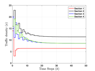
In the second approach, we start from the local abstractions , , and first compute safety controllers for each abstraction , , with local safety specification , where and for . Then we compose the local controlled components , , with an -approximate composition with given as . Then, as a final step we synthesize a safety controller for against the safety specification . The total computation time required for obtaining the safety controller using bottom-up safety synthesis is hours and minutes which is almost times faster than the monolithic synthesis case. The Figure 8 shows the evolution of traffic densities in each section of the road starting from the initial condition using controller obtained by proposed bottom-up approach. One can readily see that all the trajectories evolve within the safe region.
7. Conclusion
In this paper, we proposed a compositional abstraction-based synthesis approach for interconnected systems. We introduce a notion of approximate composition that allows composing different types of abstractions. Moreover, we provided compositional results based on approximate (alternating) simulation relation and showed how these results can be used for bottom-up safety controller synthesis. Two case studies are given to show the effectiveness of our approach. In future work, we plan to extend the bottom-up synthesis approach from safety to other types of specifications, such as reachability, stability, or more general properties described by temporal logic formulae. Another direction is to go from deterministic relationships to probabilistic ones [Aba13], which are more suitable to use when dealing with stochastic systems.
References
- [Aba13] A. Abate. Approximation metrics based on probabilistic bisimulations for general state-space markov processes: A survey. Electronic Notes in Theoretical Computer Science, 297:3–25, 2013.
- [BJP+12] R. Bloem, B. Jobstmann, N. Piterman, A. Pnueli, and Y. Saar. Synthesis of reactive (1) designs. Journal of Computer and System Sciences, 78(3):911–938, 2012.
- [BPDB18] A. Borri, G. Pola, and M. D. Di Benedetto. Design of symbolic controllers for networked control systems. IEEE Transactions on Automatic Control, 64(3):1034–1046, 2018.
- [BYG17] C. Belta, B. Yordanov, and E. A. Gol. Formal Methods for Discrete-Time Dynamical Systems. Springer International Publishing, 2017.
- [CA15] S. Coogan and M. Arcak. Efficient finite abstraction of mixed monotone systems. In Proceedings of the 18th International Conference on Hybrid Systems: Computation and Control, pages 58–67. ACM, 2015.
- [CL09] C. G. Cassandras and S. Lafortune. Introduction to discrete event systems. Springer Science & Business Media, 2009.
- [Dag94] Carlos F Daganzo. The cell transmission model: A dynamic representation of highway traffic consistent with the hydrodynamic theory. Transportation Research Part B: Methodological, 28(4):269–287, 1994.
- [DT15] E. Dallal and P. Tabuada. On compositional symbolic controller synthesis inspired by small-gain theorems. In 2015 54th IEEE Conference on Decision and Control (CDC), pages 6133–6138, 2015.
- [Fre05] G. F. Frehse. Compositional verification of hybrid systems using simulation relations. [Sl: sn], 2005.
- [GP07] A. Girard and G. J. Pappas. Approximation metrics for discrete and continuous systems. IEEE Transactions on Automatic Control, 52(5):782–798, 2007.
- [GP09] A. Girard and G. J. Pappas. Hierarchical control system design using approximate simulation. Automatica, 45(2):566–571, 2009.
- [GPT09] A. Girard, G. Pola, and P. Tabuada. Approximately bisimilar symbolic models for incrementally stable switched systems. IEEE Transactions on Automatic Control, 55(1):116–126, 2009.
- [GSB20] Kasra Ghasemi, Sadra Sadraddini, and Calin Belta. Compositional synthesis via a convex parameterization of assume-guarantee contracts. In Proceedings of the 23rd International Conference on Hybrid Systems: Computation and Control, pages 1–10, 2020.
- [HAT17] O. Hussien, A. Ames, and P. Tabuada. Abstracting partially feedback linearizable systems compositionally. IEEE Control Systems Letters, 1(2):227–232, 2017.
- [JDDBP09] A. A. Julius, A. D’Innocenzo, M. D. Di Benedetto, and G. J. Pappas. Approximate equivalence and synchronization of metric transition systems. Systems & Control Letters, 58(2):94–101, 2009.
- [JZ17] P. Jagtap and M. Zamani. QUEST: A tool for state-space quantization-free synthesis of symbolic controllers. In International Conference on Quantitative Evaluation of Systems, pages 309–313. Springer, 2017.
- [JZ20] P. Jagtap and M. Zamani. Symbolic models for retarded jump–diffusion systems. Automatica, 111:108666, 2020.
- [KAS17] E. S. Kim, M. Arcak, and S. A. Seshia. A small gain theorem for parametric assume-guarantee contracts. In Proceedings of the 20th International Conference on Hybrid Systems: Computation and Control, HSCC ’17, pages 207–216, New York, NY, USA, 2017. ACM.
- [KAZ18] E. S. Kim, M. Arcak, and M. Zamani. Constructing control system abstractions from modular components. In Proceedings of the 21st International Conference on Hybrid Systems: Computation and Control (part of CPS Week), pages 137–146. ACM, 2018.
- [KVdS10] F. Kerber and A. Van der Schaft. Compositional analysis for linear systems. Systems & Control Letters, 59(10):645–653, 2010.
- [LCGG13] E. Le Corronc, A. Girard, and G. Goessler. Mode sequences as symbolic states in abstractions of incrementally stable switched systems. In 52nd IEEE Conference on Decision and Control, pages 3225–3230. IEEE, 2013.
- [LFM+16] A. Le Coënt, L. Fribourg, N. Markey, F. De Vuyst, and L. Chamoin. Distributed synthesis of state-dependent switching control. In International Workshop on Reachability Problems, pages 119–133, 2016.
- [LP17] Ratan Lal and Pavithra Prabhakar. Safety analysis using compositional bounded error approximations of communicating hybrid systems. In 2017 IEEE 56th Annual Conference on Decision and Control (CDC), pages 2378–2383. IEEE, 2017.
- [LP19] Ratan Lal and Pavithra Prabhakar. Compositional construction of bounded error over-approximations of acyclic interconnected continuous dynamical systems. In Proceedings of the 17th ACM-IEEE International Conference on Formal Methods and Models for System Design, pages 1–5, 2019.
- [MD18] P-J. Meyer and D. V. Dimarogonas. Compositional abstraction refinement for control synthesis. Nonlinear Analysis: Hybrid Systems, 27:437–451, 2018.
- [MGW15] P-J. Meyer, A. Girard, and E. Witrant. Safety control with performance guarantees of cooperative systems using compositional abstractions. IFAC-PapersOnLine, 48(27):317–322, 2015.
- [MGW17] P-J. Meyer, A. Girard, and E. Witrant. Compositional abstraction and safety synthesis using overlapping symbolic models. IEEE Transactions on Automatic Control, 63(6):1835–1841, 2017.
- [MSSM18] K. Mallik, A-K. Schmuck, S. Soudjani, and R. Majumdar. Compositional synthesis of finite state abstractions. IEEE Transactions on Automatic Control, 2018.
- [PGT08] G. Pola, A. Girard, and P. Tabuada. Approximately bisimilar symbolic models for nonlinear control systems. Automatica, 44(10):2508–2516, 2008.
- [PPB18] G. Pola, P. Pepe, and M. D. D. Benedetto. Decentralized supervisory control of networks of nonlinear control systems. IEEE Transactions on Automatic Control, 63(9):2803–2817, 2018.
- [PPD16] G. Pola, P. Pepe, and M. D. Di Benedetto. Symbolic models for networks of control systems. IEEE Transactions on Automatic Control, 61(11):3663–3668, 2016.
- [PPDBT10] G. Pola, P. Pepe, M. D. Di Benedetto, and P. Tabuada. Symbolic models for nonlinear time-delay systems using approximate bisimulations. Systems & Control Letters, 59(6):365–373, 2010.
- [Rei11] G. Reissig. Computing abstractions of nonlinear systems. IEEE Transactions on Automatic Control, 56(11):2583–2598, 2011.
- [RWR17] G. Reissig, A. Weber, and M. Rungger. Feedback refinement relations for the synthesis of symbolic controllers. IEEE Transactions on Automatic Control, 62(4):1781–1796, 2017.
- [RZ18] M. Rungger and M. Zamani. Compositional construction of approximate abstractions of interconnected control systems. IEEE Transactions on Control of Network Systems, 5(1):116–127, 2018.
- [SGF18a] A. Saoud, A. Girard, and L. Fribourg. Contract based design of symbolic controllers for interconnected multiperiodic sampled-data systems. In 2018 IEEE Conference on Decision and Control (CDC), pages 773–779. IEEE, 2018.
- [SGF18b] A. Saoud, A. Girard, and L. Fribourg. Contract based design of symbolic controllers for vehicle platooning. In Proceedings of the 21st International Conference on Hybrid Systems: Computation and Control (part of CPS Week), pages 277–278. ACM, 2018.
- [SGF18c] A. Saoud, A. Girard, and L. Fribourg. On the composition of discrete and continuous-time assume-guarantee contracts for invariance. In 2018 European Control Conference (ECC), pages 435–440, 2018.
- [SGF20] Adnane Saoud, Antoine Girard, and Laurent Fribourg. Contract-based design of symbolic controllers for safety in distributed multiperiodic sampled-data systems. IEEE Transactions on Automatic Control, 2020.
- [SJZG18] A. Saoud, P. Jagtap, M. Zamani, and A. Girard. Compositional abstraction-based synthesis for cascade discrete-time control systems. 6th IFAC Conference on Analysis and Design of Hybrid Systems ADHS, 51(16):13 – 18, 2018.
- [SJZG20] Adnane Saoud, Pushpak Jagtap, Majid Zamani, and Antoine Girard. Compositional abstraction-based synthesis for interconnected systems: An approximate composition approach. arXiv preprint arXiv:2002.02014, 2020.
- [SNO16] Stanley W Smith, Petter Nilsson, and Necmiye Ozay. Interdependence quantification for compositional control synthesis with an application in vehicle safety systems. In 2016 IEEE 55th Conference on Decision and Control (CDC), pages 5700–5707. IEEE, 2016.
- [SZ19] A. Swikir and M. Zamani. Compositional synthesis of finite abstractions for networks of systems: A small-gain approach. Automatica, 107:551–561, 2019.
- [Tab09] P. Tabuada. Verification and control of hybrid systems: A symbolic approach. Springer Science & Business Media, 2009.
- [TI08] Y. Tazaki and J. Imura. Bisimilar finite abstractions of interconnected systems. Hybrid Systems: Computation and Control, pages 514–527, 2008.
- [TPL04] P. Tabuada, G. J. Pappas, and P. Lima. Compositional abstractions of hybrid control systems. Discrete event dynamic systems, 14(2):203–238, 2004.
- [ZA17] M. Zamani and M. Arcak. Compositional abstraction for networks of control systems: A dissipativity approach. IEEE Transactions on Control of Network Systems, 5(3):1003–1015, 2017.
- [ZPMT12] M. Zamani, G. Pola, M. Mazo, and P. Tabuada. Symbolic models for nonlinear control systems without stability assumptions. IEEE Transactions on Automatic Control, 57(7):1804–1809, 2012.
- [ZSGF19a] D. Zonetti, A. Saoud, A. Girard, and L. Fribourg. Decentralized monotonicity-based voltage control of dc microgrids with zip loads. IFAC-PapersOnLine, 52(20):139–144, 2019.
- [ZSGF19b] D. Zonetti, A. Saoud, A. Girard, and L. Fribourg. A symbolic approach to voltage stability and power sharing in time-varying dc microgrids. In European Control Conference (ECC), 2019.
- [ZTA17] M. Zamani, I. Tkachev, and A. Abate. Towards scalable synthesis of stochastic control systems. Discrete Event Dynamic Systems, 27(2):341–369, 2017.