Two intermediate-mass transiting brown dwarfs from the TESS mission

Abstract

We report the discovery of two intermediate-mass transiting brown dwarfs (BDs), TOI-569b and TOI-1406b, from NASA’s Transiting Exoplanet Survey Satellite mission. TOI-569b has an orbital period of $P=6.55604\pm 0.00016$ days, a mass of $M_{b}=$ $64.1\pm 1.9$$\,{\rm M_{J}}$, and a radius of $R_{b}=$ $0.75\pm 0.02$$\,{\rm R_{J}}$. Its host star, TOI-569, has a mass of $M_{\star}=$ $1.21\pm 0.05$$\,{\rm M_{\odot}}$, a radius of $R_{\star}=$ $1.47\pm 0.03$$\,{\rm R_{\odot}}$, $\rm[Fe/H]=+0.29\pm 0.09$ dex, and an effective temperature of $T_{\rm eff}=$ $5768\pm 110$K. TOI-1406b has an orbital period of $P=10.57415\pm 0.00063$ days, a mass of $M_{b}=$ $46.0\pm 2.7$$\,{\rm M_{J}}$, and a radius of $R_{b}=$ $0.86\pm 0.03$$\,{\rm R_{J}}$. The host star for this BD has a mass of $M_{\star}=$ $1.18\pm 0.09$$\,{\rm M_{\odot}}$, a radius of $R_{\star}=$ $1.35\pm 0.03$$\,{\rm R_{\odot}}$, $\rm[Fe/H]=-0.08\pm 0.09$ dex, and an effective temperature of $T_{\rm eff}=$ $6290\pm 100$K. Both BDs are in circular orbits around their host stars and are older than 3 Gyr based on stellar isochrone models of the stars. TOI-569 is one of two slightly evolved stars known to host a transiting BD (the other being KOI-415). TOI-1406b is one of three known transiting BDs to occupy the mass range of 40-50$\,{\rm M_{J}}$ and one of two to have a circular orbit at a period near 10 days (with the first being KOI-205b). Both BDs have reliable ages from stellar isochrones in addition to their well-constrained masses and radii, making them particularly valuable as tests for substellar isochrones in the BD mass-radius diagram.

1 Introduction

Brown dwarfs (BDs) are traditionally defined as objects with masses between 13 and 80 Jupiter masses ($\,{\rm M_{J}}$) and, for those that orbit main-sequence stars, are typically observed to be 0.7 to 1.4 Jupiter radii ($\,{\rm R_{J}}$) in size (Csizmadia & CoRot Team, 2016; Carmichael et al., 2019). The lower mass limit that separates planets from BDs corresponds to the threshold required to fuse deuterium in the core of the BD, which, in detail, is $11-16\,{\rm M_{J}}$ depending on the metallicity of the BD (Spiegel et al., 2011). The threshold to fuse hydrogen in the core is $75-80\,{\rm M_{J}}$ and this separates BDs from stars. This higher threshold depends on the initial formation conditions and how convection affects the object (Baraffe et al., 2002). The mass and radius of a BD are measured through a combination of observational techniques, with the most important being radial velocity (RV) measurements and transit photometry of the host star.

This is where the Transiting Exoplanet Survey Satellite (TESS) mission plays a major role. The transit method has been most successful in the characterization of BDs in relatively short orbital periods (on the order of 10 to 20 days or less to detect multiple transits), which is why the TESS mission has been particularly useful in making the initial detections of recently discovered transiting BDs (e.g. Subjak et al., 2019; Jackman et al., 2019). The transit light curves from TESS are taken over roughly 28 consecutive days per sector (or up to one year for overlapping sectors), with occasional gaps in coverage due to data downloads and instrumental anomalies. These light curves give an estimate of the radius of the candidate companions relative to the radius of the star. This informs us on whether or not a candidate companion is within the typical range of radii expected for a BD orbiting a main-sequence star. We are particularly fortunate at the present time to be able to utilize the parallax measurements from Gaia DR2 (Gaia Collaboration et al., 2018) to derive precise stellar distances and radii for stars that host transiting BDs.

Though TESS and Gaia provide us with some handle on the radius of a BD, follow up spectra are needed to accumulate a series of RV measurements to determine an orbit and measure a mass. This is an important step as objects ranging from roughly $1\,{\rm M_{J}}$ to $100\,{\rm M_{J}}$ may have the same radius ($\sim$1$\,{\rm R_{J}}$), so the only way to distinguish them is through a mass measurement. Since the masses of transiting BDs produce large RV signals around typical FGK main sequence stars, RV follow up of these BDs is fairly accessible (especially given the precision of modern echelle spectrographs).

When comparing the detection of transiting BDs to the detection of transiting giant planets, we see two facts emerge: 1) for host stars with similar radii, transiting BDs should be roughly as easy to detect as hot Jupiters given both types of objects are similar in size and given the photometric precision and sensitivity of transit survey missions like TESS. 2) for host stars of similar masses, it is as easy or easier to characterize the mass of a BD given that they are more massive and produce larger RV signals than giant planets. Despite this, we know of only 23 transiting BDs (see Table 7 for a list). When compared to the number of known transiting hot Jupiters and even eclipsing low-mass stellar companions in comparable orbital periods, it is easy to see that there is a lack of transiting BDs; this is the so-called “brown dwarf desert” (Marcy & Butler, 2000). Though not yet clear, this “desert” may result from the distributions of the two different formation mechanisms (one for planets and one for stars) tailing off—and perhaps overlapping—somewhere within the nominal BD mass range.

To understand this population on a deeper level, we use the mass, radius, and age of transiting BDs to examine how these substellar objects evolve compared to substellar evolutionary models (e.g. Baraffe et al., 2003). Since a BD may only fuse deuterium and not hydrogen, it lacks the energy source needed to stave off gravitational contraction on long timescales as effectively as stars do, so the BD’s radius will shrink as it ages. This is why the age is important in addition to mass and radius. If we can reliably determine the age of a star that hosts a transiting BD, whether through an association with a star cluster, gyrochronology, or asteroseismology, then we may use that transiting BD to test substellar evolutionary models in mass, radius, and age parameter spaces. This assumes that both the host star and the transiting BD form at the same time. So far, only 3 BDs transiting main sequence stars with well-determined ages are known (Beatty et al., 2018; David et al., 2019; Gillen et al., 2017), so we are lacking test points on the substellar mass-radius diagram with precisely determined mass, radius, and age.

Table 1: Coordinates and magnitudes for TOI-569 and TOI-1406. The values here make up the spectral energy distributions used to model the stars.

	Description	TOI-569	TOI-1406	Source
$\alpha_{\rm J2000}$	Equatorial	07 40 24.67	05 28 30.71	1
$\delta_{\rm J2000}$	coordinates	-42 09 16.79	-48 24 32.64	1
$T$	TESS $T$	$9.473\pm 0.006$	$11.427\pm 0.006$	2
$G$	Gaia $G$	$9.936\pm 0.001$	$11.759\pm 0.001$	1
$B_{T}$	Tycho $B_{T}$	$11.036\pm 0.048$	$13.352\pm 0.359$	3
$V_{T}$	Tycho $V_{T}$	$10.173\pm 0.032$	$12.074\pm 0.195$	3
$J$	2MASS $J$	$8.829\pm 0.020$	$10.929\pm 0.020$	4
$H$	2MASS $H$	$8.575\pm 0.060$	$10.787\pm 0.030$	4
$K_{S}$	2MASS $K_{S}$	$8.444\pm 0.020$	$10.675\pm 0.020$	4
WISE1	WISE 3.4$\rm\mu m$	$8.419\pm 0.023$	$10.649\pm 0.023$	5
WISE2	WISE 4.6$\rm\mu m$	$8.467\pm 0.020$	$10.692\pm 0.021$	5
WISE3	WISE 12$\rm\mu m$	$8.414\pm 0.021$	$10.651\pm 0.062$	5
WISE4	WISE 22$\rm\mu m$	$8.180\pm 0.188$	-	5

Note. — References: 1 - Lindegren et al. (2018), corrected from the J2015 epoch, 2 - Stassun et al. (2018b), 3 - Høg et al. (2000), 4 - Cutri et al. (2003), 5 - Cutri & et al. (2013)

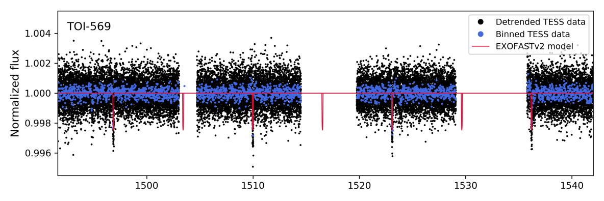
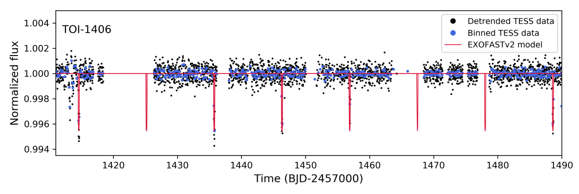
Figure 1: Top: Detrended TESS light curve of TOI-569 in the black points. The star was observed at 2 minutes cadence in TESS sectors 7 and 8 and the binning shown here in the blue points uses bin sizes of 45 minutes. This star also exhibits periodic 1-3% flux variations likely due to star spots based on the changes in the patterns of the modulation; these effects have been removed for the transit analysis. Bottom: Detrended TESS light curve of TOI-1406 (black points) obtained from the full-frame images at 30 minute cadence from TESS sectors 4, 5, and 6 with the bin sizes at a length of 90 minutes (blue points).

Here we report the discovery and characterization of two new transiting BDs with reliable mass, radius, and age measurements: TOI-569b and TOI-1406b. TOI-569b orbits a recently evolved star in a circular orbit. TOI-1406b orbits an F-type star, joining 7 other transiting BDs that orbit F-type stars, and is also in a circular orbit. These both serve as new test points on the mass-radius diagram for BDs older than 3 Gyr. In Section 2, we give details on the light curves and spectra that were obtained for this study with additional attention given to the determination of the orbital period of TOI-569b, which was initially reported incorrectly as twice its actual value due to gaps in the TESS data. Section 3 describes the analysis techniques used to derive the host star and BD properties. Section 4 contains discussion of the implications of these new discoveries in the BD mass-radius diagram as these two transiting BDs are the oldest transiting BDs that have been well-characterized.

2 Observations

2.1 TESS and ground-based light curves

The light curves of TOI-569 come from the TESS mission in sectors 7 and 8, and the Las Cumbres Observatory (LCOGT). For the TESS light curve for TOI-569, we use the Pre-search Data Conditioning Simple Aperture Photometry flux (PDCSAP; Stumpe et al., 2014; Smith et al., 2012) from the Mikulski Archive for Space Telescopes (MAST). The PDCSAP light curve has systematic effects removed and with this, we then normalize the light curve with the lightkurve package in Python (the Lightkurve Collaboration et al., 2018). The light curves used for TOI-1406 come from the full-frame images (30 minute cadence) from the TESS mission in sectors 4, 5, and 6. We use the lightkurve package to extract and normalize the light curve of TOI-1406.

For the light curve extraction, we use circular apertures that are fixed to the target star’s position for each sector. When the star moves slightly between sectors, the aperture is moved to follow it. The counts from each pixel within the aperture are summed and the resulting light curve is detrended using the lightkurve package’s built-in flattening tool, which we use to remove stellar rotational variability, when present, as well as scattered background light. The detrended TESS light curves are shown in Figure 1.

We observed an ingress of TOI-569 continuously for 140 minutes on April 15, 2019 using 15 s exposures and a z-short band filter from the LCOGT (Brown et al., 2013) 1.0 m node at Cerro Tololo Inter-American Observatory. We used the TESS Transit Finder, which is a customized version of the Tapir software package (Jensen, 2013), to schedule our transit observations. The $4096\times 4096$ LCOGT SINISTRO cameras have an image scale of 0.389$\arcsec$ per pixel, resulting in a $26\arcmin\times 26\arcmin$ field of view. The images were calibrated by the standard LCOGT BANZAI pipeline, and photometric data were extracted with the AstroImageJ software package (Collins et al., 2017) using a circular aperture with radius 5.8$\arcsec$. The images have typical stellar point-spread-functions with a half-width-half-maximum of 1$\arcsec$. We detect a $\sim 3000$ ppm ingress on target with apertures as small as 2$\arcsec$ in radius. Systematic effects start to dominate the light curve for smaller apertures. Thus, we confirm that the source of the TESS detection is within 3$\arcsec$ of the target star location and that the transit depth from the LCOGT partial transit is consistent with the TESS depth for all aperture radii we checked down to 2$\arcsec$. We did not obtain any ground-based photometric followup of TOI-1406.

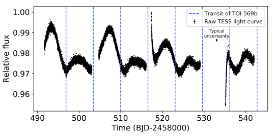
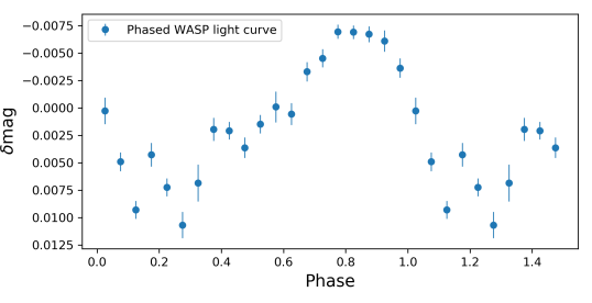
Figure 2: Top: Offset-normalized raw TESS light curve from sectors 7 and 8 of TOI-569. The offset between each sector is removed using lightkurve, but no other systematic effects are removed since the focus of this figure is to show the missed transits of TOI-569b and provide context for the flux variability of the host star. The rapid ramp down at 515 days and ramp up at 535 days are instrumental systematics from the spacecraft. The blue dashed lines show the transit times predicted by the final model ephemeris for TOI-569b. Bottom: WASP light curve of TOI-569 phase folded at 13.03 days from observations taken over a span of 150 days.

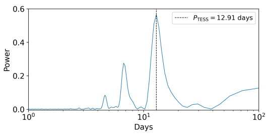
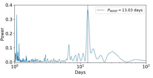
Figure 3: Top: Lomb-Scargle periodogram from the TESS light curve of TOI-569. Bottom: Lomb-Scargle periodogram from the WASP light curve of TOI-569. Both the WASP and TESS periodograms indicate a peak frequency near 13 days. The peak in the lower panel is narrower because the total time coverage from the WASP data was nearly 3 times longer than that from TESS.

2.1.1 Light curve modulation and the orbital period of the TOI-569 system

Previous to the transit detections of TOI-569b from TESS, the Wide Angle Search for Planets (WASP) found a 13-day modulation in the light curve of TOI-569. The phased light curve for WASP is shown in Figure 2. The WASP data were taken during the 2011 to 2012 seasons with a 150-day span of coverage. The transits of TOI-569b are too shallow to be detected in the WASP light curve even when phase folded to the ephemeris from TESS, but they can be seen in the TESS light curve in the top panel of Figure 2. The WASP and TESS light curves show a similar but not exactly equal modulation. The periodic peaks and dips in both light curves are likely from brightness variations due to star spots, which are known to vary over time. The unevenness in the peaks in the TESS light curves are likely from multiple different star spot configurations on different areas on the surface of the star in addition to the evolution of spot brightness over time.

The gaps in the TESS light curve occur during every other transit of TOI-569b in the sectors the host star was observed. This is the reason why the initial orbital period was reported to be 13.12 days (twice the true orbital period of 6.56 days). We discovered that this was the case as the orbital solution developed with RV follow up using the instruments described in later sections. It seems coincidental that this erroneous orbital period of 13.12 days is nearly equal to the 13-day modulation in the WASP light curve. This made the BD appear to have an orbit synchronized with the rotation rate of the star, but this turned out not to be the case upon a more thorough investigation that accounts for the orbital solution derived from RVs. We note that the observation of the transit of TOI-569b with the LCOGT 1-meter telescope did not occur at opposite parity to the transits detected by TESS, so we cannot use this to independently confirm the 6.56-day period of TOI-569b.

Using a Lomb-Scargle periodogram analysis on both the TESS and WASP light curves separately, we see a peak frequency at roughly 13 days (12.91 days for TESS and 13.01 days for WASP). This may suggest that TOI-569 and its companion BD are in a 2:1 spin-orbit resonance.

Table 2: Nearby sources from Gaia DR2 data. This table list sources within $30\arcsec$ of each star (TOI-569 and TOI-1406) that are $G<16$ in magnitude. Listing sources fainter than this results in too many items to reasonably list here. The parallaxes ($\pi$) and proper motions ($\mu_{\rm\alpha}$, $\mu_{\rm\delta}$) of the nearby stars indicate that none are associated with TOI-569 or TOI-1406.

Gaia DR2 ID	$\alpha$ (J2000)	$\delta$ (J2000)	$\pi$ (mas)	$\mu_{\rm\alpha}$ (mas/yr)	$\mu_{\rm\delta}$ (mas/yr)	$G$ (mag)
5535473358555685760 (TOI-569)	07 40 24.67	-42 09 16.79	$6.3723\pm 0.0306$	$6.317\pm 0.053$	$-3.068\pm 0.048$	9.94
5535473392915426304	07 40 26.44	-42 09 00.02	$0.0899\pm 0.0193$	$-1.790\pm 0.035$	$2.832\pm 0.030$	13.69
5535473358555686656	07 40 23.61	-42 09 39.57	$0.8838\pm 0.0275$	$12.130\pm 0.047$	$-13.344\pm 0.041$	14.88
5535473358556195840	07 40 23.25	-42 09 38.38	$0.1963\pm 0.0414$	$-4.600\pm 0.072$	$5.585\pm 0.060$	15.64
4797030079342886784 (TOI-1406)	05 28 30.71	-48 24 32.64	$2.3855\pm 0.0291$	$0.889\pm 0.057$	$-21.885\pm 0.066$	11.76
4797030079342886656	05 28 29.07	-48 24 41.93	$1.1846\pm 0.0396$	$1.222\pm 0.073$	$-1.752\pm 0.093$	15.78

2.2 High resolution imaging and contaminating sources

Though the LCOGT data give us a sense of whether or not the transit signals for TOI-569 are within roughly 3$\arcsec$ of the target star, we may use speckle imaging to confirm whether or not there is contamination even closer to the target. For TOI-569, we used SOAR speckle imaging to look for other objects within the TESS aperture that would significantly contaminate the transit and RV signals we observe. Nearby stars which fall within the same TESS image profile as the target can cause photometric contamination or be the source of an astrophysical false positive, such as a background or nearby eclipsing binary star. We searched for nearby sources to TOI-569 with SOAR speckle imaging (Tokovinin, 2018) on May 18, 2019, observing in a similar visible bandpass as TESS (the Cousins-I band). Further details of the observations are available in Ziegler et al. (2019). We detected no nearby stars within 3$\arcsec$ of TOI-569. The 5-$\sigma$ detection sensitivity and the speckle auto-correlation function from the SOAR observation are plotted in Figure 4.

We also use data from Gaia DR2 (Gaia Collaboration et al., 2018) to gather a census of nearby stars, finding that no stars brighter than G=17.0 are within 25$\arcsec$ and only two stars with G=13.7 and G=14.9 are approximately 26$\arcsec$ from TOI-569, which has a brightness of G=9.9 (Table 2). These other fainter stars also do not share the same proper motion as TOI-569, which indicates that they are not associated with TOI-569 and are more distant background stars.

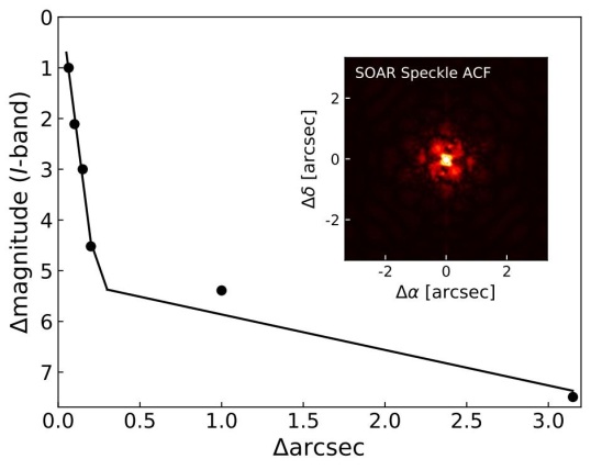
Figure 4: The 5-$\sigma$ sensitivity limits and auto-correlation functions of the SOAR speckle observations of TOI-569. The black circles are measured data points and the lines are fits in two different separation regimes. In general, the sensitivity of speckle imaging to companions rises sharply from the diffraction limit to a “knee” at a separation of $0.15-0.2\arcsec$, where it then continues to slowly increase out to ∼1.5″, beyond which the speckle patterns begin to become de-correlated. No nearby contaminating sources are detected within 3$\arcsec$.

We do not have any high resolution imaging (as in, sub-$3\arcsec$ coverage) for TOI-1406, but using Gaia DR2 data, we find only 3 other stars within 30$\arcsec$ of TOI-1406. The brightest of these other stars has a magnitude of G=15.8 and is 19$\arcsec$ from TOI-1406, which has a magnitude of G=11.8. We also find that none of these other stars share the same proper motion as TOI-1406 from the Gaia DR2 data (Table 2).

2.3 CHIRON spectra

To characterize the RVs and stellar atmospheric parameters of TOI-569 and TOI-1406, we obtained a series of spectroscopic observations using the CHIRON spectrograph on the 1.5 m SMARTS telescope (Tokovinin et al., 2013), located at Cerro Tololo Inter-American Observatory, Chile. CHIRON is a high resolution echelle spectrograph that is fed via an image slicer and a fiber bundle. CHIRON achieves a spectral resolving power of $\lambda/\Delta\lambda\equiv R\sim 80,000$ over the wavelength region 4100 to $8700$ Å. The wavelength calibration is obtained via thorium-argon hollow-cathode lamp exposures that bracket each stellar spectrum.

To derive the stellar RVs, we performed a least-squares deconvolution (Donati et al., 1997) between the observed spectra and a non-rotating synthetic template generated via ATLAS9 atmospheric models (Castelli & Kurucz, 2004) at the stellar atmospheric parameters of each target. We then model the stellar line profiles derived from the least-squares deconvolution via an analytic rotational broadening kernel as per Gray (2005). This procedure follows that done in Zhou et al. (2019). The derived RVs for TOI-569 and TOI-1406 are listed in Table 3 and this series of RVs helped to reveal the true orbital period of the BD. The stellar parameters derived from the spectra of TOI-569 are $T_{\rm eff}=5669\pm 106$K, $\log{g}=4.11\pm 0.18$, $\rm[Fe/H]=+0.23\pm 0.05$ dex, and $v\sin{I_{\star}}=5.33\pm 0.50$ $\rm km\,s^{-1}$. For TOI-1406, we find $T_{\rm eff}=6347\pm 186$K, $\log{g}=4.09\pm 0.15$, $\rm[Fe/H]=-0.05\pm 0.11$ dex, and an approximate full width at half max for the line broadening profile of $\rm FWHM=12.91\pm 0.24$ $\rm km\,s^{-1}$ with the CHIRON spectra. For TOI-569, we take care to account for the instrumental profile and macroturbulence to extract $v\sin{I_{\star}}$ from the FWHM approximation ($\rm FWHM=6.65\pm 0.5$ $\rm km\,s^{-1}$) with CHIRON as this is important in our analysis of the stellar inclination in Section 3.3.

Table 3: Relative radial velocities, bisector span ($V_{\rm span}$), and FWHM of TOI-569 from CHIRON, CORALIE, and FEROS and of TOI-1406 from CHIRON and ANU.

$\rm BJD_{\rm TDB}-2450000$	RV ($\rm m\,s^{-1}$)	$\sigma_{\rm RV}$ ($\rm m\,s^{-1}$)	$V_{\rm span}$ ($\rm km\,s^{-1}$)	FWHM ($\rm km\,s^{-1}$)	Instrument	Target
8594.61690	75132.3	16.6	-	6.93	CHIRON	TOI-569
8606.50771	77754.5	20.7	-	6.67	CHIRON	TOI-569
8596.60327	66265.0	18.9	-	7.00	CHIRON	TOI-569
8595.59076	69864.3	16.4	-	6.67	CHIRON	TOI-569
8607.53323	75982.6	17.8	-	6.73	CHIRON	TOI-569
8611.59733	71966.8	24.9	-	6.65	CHIRON	TOI-569
8612.57581	76679.3	30.6	-	6.57	CHIRON	TOI-569
8649.44500	66193.1	24.2	-	6.63	CHIRON	TOI-569
8651.48774	74957.8	34.9	-	6.81	CHIRON	TOI-569
8654.46711	70453.9	27.2	-	6.40	CHIRON	TOI-569
8593.58587	79347.5	13.0	$-0.030$	10.55	CORALIE	TOI-569
8597.47058	68533.2	31.6	$0.089$	10.48	CORALIE	TOI-569
8599.52446	78333.6	16.8	$-0.023$	10.48	CORALIE	TOI-569
8602.58567	69230.9	13.3	$0.001$	10.46	CORALIE	TOI-569
8603.46595	67533.0	20.3	$-0.012$	10.47	CORALIE	TOI-569
8614.49353	75527.3	32.4	$0.004$	10.43	CORALIE	TOI-569
8615.48815	70140.4	29.5	$0.060$	10.66	CORALIE	TOI-569
8594.49170	77148.3	6.5	$0.019$	-	FEROS	TOI-569
8595.52217	71681.8	8.4	$0.015$	-	FEROS	TOI-569
8597.51010	68686.8	6.8	$0.015$	-	FEROS	TOI-569
8617.52568	70033.1	6.0	$0.009$	-	FEROS	TOI-569
8533.07797	-19568.3	465.0	-	-	ANU	TOI-1406
8534.98787	-17679.4	197.8	-	-	ANU	TOI-1406
8536.06364	-15764.1	260.2	-	-	ANU	TOI-1406
8537.96961	-12090.1	725.7	-	-	ANU	TOI-1406
8538.93516	-12135.5	282.9	-	-	ANU	TOI-1406
8561.89365	-13798.5	270.0	-	-	ANU	TOI-1406
8540.61381	-13631.0	69.2	-	12.91	CHIRON	TOI-1406
8541.60193	-15950.3	91.8	-	12.69	CHIRON	TOI-1406
8542.56709	-17888.9	45.1	-	13.07	CHIRON	TOI-1406
8544.52353	-19087.2	166.4	-	12.78	CHIRON	TOI-1406
8546.51779	-15936.1	91.8	-	12.81	CHIRON	TOI-1406
8562.57958	-15177.2	126.9	-	12.89	CHIRON	TOI-1406
8566.55925	-18101.1	97.7	-	12.77	CHIRON	TOI-1406
8567.59295	-16029.1	83.6	-	12.82	CHIRON	TOI-1406
8568.54388	-13973.3	124.3	-	13.36	CHIRON	TOI-1406
8569.57364	-12432.3	110.3	-	12.98	CHIRON	TOI-1406

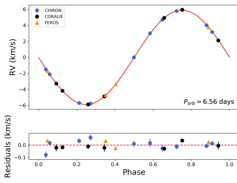
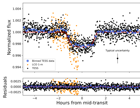
Figure 5: Top: Relative radial velocities of TOI-569 with EXOFASTv2 orbital solution plotted in red. The orbital eccentricity is consistent with zero ($e<0.0035$, 1-$\sigma$ upper limit). Bottom: TESS (black) and LCOGT 1-meter (orange) light curves with EXOFASTv2 transit model in red and binned TESS data in blue.

2.4 ANU 2.3m echelle spectra

To help confirm TOI-1406b as a BD, we obtained six spectroscopic observations with the echelle spectrograph on the Australian National University (ANU) 2.3 m telescope, located at Siding Spring Observatory, Australia. The ANU 2.3 m echelle is a slit-fed spectrograph that yields a resolving power of $R\sim 23,000$ over the wavelength region of $\rm 3700-6700\,\AA$. Wavelength calibration was provided by bracketing thorium-argon lamp exposures, and the spectra were reduced as per Zhou et al. (2014). The RVs from each exposure were measured via the least-squares deconvolution technique as described in Section 2.3. To derive $T_{\rm eff}$, $\log{g}$, and $\rm[Fe/H]$ for TOI-1406, we use SpecMatch-emp (Yee et al., 2017), which matches the input spectra to a library of stars with well-determined parameters derived with a variety of independent methods, e.g., interferometry, optical and NIR photometry, asteroseismology, and LTE analysis of high-resolution optical spectra. From the ANU spectra and SpecMatch-emp we find $T_{\rm eff}=6283\pm 110$K, $\log{g}=4.13\pm 0.12$, $\rm[Fe/H]=-0.09\pm 0.09$ dex and $\rm FWHM=15.0\pm 1.0$ $\rm km\,s^{-1}$ for TOI-1406.

2.5 CORALIE spectra

TOI-569 was observed with the CORALIE spectrograph on the Swiss 1.2 m Euler telescope at La Silla Observatories, Chile (Queloz et al., 2001), between April 19 and May 11, 2019. CORALIE has a resolving power of $R\sim 60,000$ and is fed by two fibers; one 2″ diameter on-sky science fiber encompassing the star and another which can either be connected to a Fabry-Pérot etalon for simultaneous wavelength calibration or on-sky for background subtraction of the sky-flux. RVs were computed for each epoch by cross-correlating with a binary G2 mask (Pepe et al., 2002). Bisector-span, full-width half-max, and other line-profile diagnostics were computed as well using the standard CORALIE data reduction software. Exposure times ranged from 450 s to 1200 s. We obtain internal error estimates of 13-32 $\rm m\,s^{-1}$. The resulting velocities are plotted in Figure 5, and are listed in Table 3.

The CORALIE spectra were shifted to the stellar rest frame and stacked while weighting the contribution from each spectrum with its mean flux to produce a high signal-to-noise spectrum for spectral characterization using SpecMatch-emp (Yee et al., 2017). We used the spectral region around the Mgb triplet ($5100-5340{\rm\AA}$) to match our spectrum to the library spectra through $\chi^{2}$ minimization. A weighted linear combination of the five best matching spectra were used to extract bulk stellar parameters; $T_{\rm eff}=5481\pm 110$K, $\log{g}=4.08\pm 0.12$ and $\rm[Fe/H]=+0.41\pm 0.09$ dex for TOI-569.

2.6 FEROS spectra

TOI-569 was observed with the FEROS spectrograph (Kaufer & Pasquini, 1998) mounted on the MPG 2.2 m telescope installed at the ESO La Silla Observatory. Four spectra were obtained between April 20 and May 14, 2019. Observations were performed with the simultaneous calibration mode where a second fiber is illuminated with a thorium-argon lamp for tracking the instrumental drift in RV during the science exposure. The adopted exposure time was of 400s which produced spectra with a typical signal-to-noise ratio per resolution element of 90. FEROS data were processed with the ceres pipeline (Brahm et al., 2017a), which performs the optimal extraction of the raw data, the wavelength calibration, the instrumental drift correction, and the computation of precise RVs and bisector spans. The results are presented in Table 3. The four FEROS spectra were combined in order to measure the atmospheric parameters using the zaspe package (Brahm et al., 2017b), obtaining $T_{\rm eff}$ = 5669 $\pm$ 80 K, $\log{g}$ = 4.21 $\pm$ 0.12, $\rm[Fe/H]=+0.28\pm 0.05$ dex, and an approximate $\rm FWHM=6.45\pm 0.30$ $\rm km\,s^{-1}$ for TOI-569.

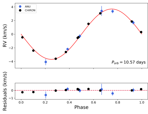
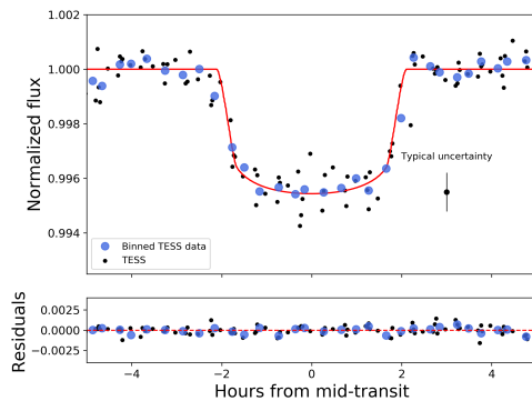
Figure 6: Top: Relative radial velocities of TOI-1406 with EXOFASTv2 orbital solution plotted in red. The orbital eccentricity is consistent with zero ($e<0.039$, 1-$\sigma$ upper limit). Bottom: TESS light curve with EXOFASTv2 transit model in red and binned TESS data in blue.

Table 4: Spectroscopic values for TOI-569 and TOI-1406 from CHIRON, ANU, CORALIE, and FEROS. We use [Fe/H] and $T_{\rm eff}$ values from CHIRON as inputs to the global model described in Section 3.1.

TOI-569	CHIRON	CORALIE	FEROS
$T_{\rm eff}$ (K)	$5669\pm 106$	$5481\pm 110$	$5669\pm 80$
$\log{g}$	$4.11\pm 0.18$	$4.08\pm 0.12$	$4.21\pm 0.12$
$\rm[Fe/H]$ (dex)	$+0.23\pm 0.05$	$+0.41\pm 0.09$	$+0.28\pm 0.05$
FWHM ($\rm km\,s^{-1}$)	$6.65\pm 0.16$	$10.50\pm 0.50$	$6.45\pm 0.30$
$R$ (resolution)	80,000	60,000	48,000
TOI-1406	ANU	CHIRON
$T_{\rm eff}$ (K)	$6283\pm 110$	$6347\pm 186$	-
$\log{g}$	$4.13\pm 0.12$	$4.09\pm 0.15$	-
$\rm[Fe/H]$ (dex)	$-0.09\pm 0.09$	$-0.05\pm 0.11$	-
FWHM ($\rm km\,s^{-1}$)	$15.0\pm 1.0$	$12.9\pm 0.2$	-
$R$ (resolution)	23,000	80,000	-

3 Analysis

3.1 Modeling with EXOFASTv2

The masses and radii of the BDs are derived using EXOFASTv2. A full description of EXOFASTv2 is given in Eastman et al. (2019). EXOFASTv2 uses the Monte Carlo-Markov Chain (MCMC) method. For each MCMC fit, we use N=36 (N = 2$\times n_{\rm parameters}$) walkers, or chains, and run for 50,000 steps, or links. To derive stellar parameters, EXOFASTv2 utilizes the MIST isochrone models (Dotter, 2016; Choi et al., 2016; Paxton et al., 2015).

The parameters for which we set priors and the types of priors we set for each (i.e. uniform $\mathcal{U}[a,b]$ or Gaussian $\mathcal{G}[a,b]$) are shown in Tables 8 and 9. We rely on our spectroscopic measurements of [Fe/H] and $T_{\rm eff}$ and parallax measurements from Gaia to define our Gaussian priors, which penalize the fit for straying beyond the width, $b$, away from the mean, $a$ of the parameter. We use an upper limit for the $A_{V}$ extinction. See Table 3 of Eastman et al. (2019) for a detailed description of priors in EXOFASTv2. For the choice of priors for [Fe/H] and $T_{\rm eff}$, we use the CHIRON values since CHIRON has the highest spectral resolution $R=80,000$ of the spectrographs we used (see Table 4). The resulting EXOFASTv2 values are consistent with the input values from CHIRON. The spectral energy distribution for each star is also taken into account with EXOFASTv2 and are shown in Figure 8. The BD parameters are derived with the normalized TESS and LCOGT light curves and non-phase folded RVs into EXOFASTv2 as inputs. The non-negligible BD mass is properly accounted for in EXOFASTv2, so no particularly special treatment is needed with regard to deriving the companion masses.

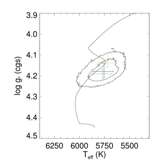
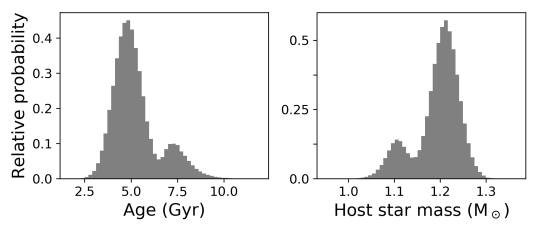
Figure 7: Top: MIST isochrone from EXOFASTv2 for TOI-569. The best-fitting MIST track is shown by the black line. The median values and 1-$\sigma$ errors from our global fit are shown in the black cross with the corresponding 3-$\sigma$ contours in black. When splitting this bimodal global solution (black points and contours), the results are the blue and orange crosses. The blue cross shows the higher probability solution for $\log{g}$ and $T_{\rm eff}$ and the orange cross shows the lower probability solution. Bottom: Age and stellar mass posterior distributions from EXOFASTv2 for TOI-569. We show these to provide a sense of the relative probabilities between the peaks of the bimodal distributions, which is roughly 3-to-1 in favor of a more massive, younger system (blue cross in top panel). We see no bimodality for the posterior distributions of TOI-1406 in EXOFASTv2.

We see bimodality in the posterior distribution for the age (and correlated parameters) of TOI-569, so we present the two most probable solutions resulting from the bimodal posterior distributions with the absolute most probable solution taken as the final adopted value (Table 9). The most relevant bimodal posterior distributions are shown in Figure 7. The probability of the solution, for age and mass, we report here is 0.73, with the less likely solution having a probability of 0.27.

The resulting stellar SED models from EXOFASTv2 for TOI-569 and TOI-1406 are shown in Figure 8. These follow the procedures outlined in Stassun & Torres (2016); Stassun et al. (2017, 2018a).

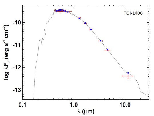
Figure 8: Spectral energy distributions for TOI-569 and TOI-1406. Red symbols represent the observed photometric measurements, where the horizontal bars represent the effective width of the bandpass. Blue symbols are the model fluxes from the best-fit Kurucz atmosphere model (black).

3.2 Analysis with pyaneti

As an independent check on our EXOFASTv2 analysis, we also carried out an analysis with the pyaneti (Barragán et al., 2019a) software. Using a Bayesian approach combined with MCMC sampling, we performed a joint analysis of the RV measurements and the TESS light curves and modelled posterior distributions of the fitted parameters. The RV data were fitted with Keplerian orbits, and for each different instrumental set-up, an offset term for each systemic velocity is included. The non-negligible mass of the brown dwarf is properly taken into account in pyaneti (Barragán et al., 2019b). The photometric data are modeled with the quadratic limb-darkening model of Mandel & Agol (2002).

We use uniform priors and fit for the BD-to-star radius ratio, the orbital period, the mid-transit time, the scaled orbital distance, the eccentricity, the argument of periastron, the impact parameter ($b$), and the Doppler semi-amplitude variation ($K$). The allowed ranges for the fit parameters for pyaneti are shown in Table 5.

Table 5: Allowed ranges for fit parameters from pyaneti.

Parameter	TOI-569	TOI-1406
$R_{\rm BD}/R_{\star}$	[0, 0.1]	[0, 0.1]
$P_{\rm orb}$ (days)	[6.5541, 6.5580]	[10.5721, 10.5762]
$T_{0}-2458400$ ($\rm BJD_{TDB}$)	[96.858, 96.878]	[14.5061, 14.7061]
$a/R_{\star}$	[1.1, 12]	[1.1, 19]
$e\cos{\omega}$	[-1, 1]	[-1, 1]
$e\sin{\omega}$	[-1, 1]	[-1, 1]
Impact parameter $b$	[0, 1]	[0, 1]
Semi-amplitude $K$ ($\rm km\,s^{-1}$)	[0, 15]	[0, 15]

We used 500 independent chains, and checked for convergence after every 5,000 iterations. After convergence, a posterior distribution of 250,000 independent points for every parameter was computed from the last 500 iterations. We find the eccentricity to be consistent with zero for both BDs. We find a mass and radius of TOI-569b and TOI-1406b to be consistent within 1-$\sigma$ of the values from the EXOFASTv2 models.

3.3 Rotational inclination angle of TOI-569

Astronomers may calculate the angle at which a star is inclined to the line-of-sight, $I_{\star}$, in order to learn about the relative alignment between this angle and the orbital inclination angle, $i$, of a transiting or eclipsing object. Using the spectroscopic $v\sin{I_{\star}}$ measurement from CHIRON (the highest resolution spectrograph we used with $R\sim 80,000$) and the $P_{\rm rot}$ results from the Lomb-Scargle periodogram analysis, we calculate the inclination of the rotational axis of TOI-569 to be $I_{\star}=65.58^{+17.75}_{-8.55}$ ^∘ (1-$\sigma$ uncertainties). This is traditionally done by taking:

$$I_{\star}=\sin^{-1}\left(\frac{v\sin{I_{\star}}}{V_{\rm rot}}\right)$$ (1)

where $v\sin{I_{\star}}=5.33\pm 0.50$ $\rm km\,s^{-1}$ and $V_{\rm rot}=2\pi R_{\star}/P_{\rm rot}=5.80\pm 0.58$ $\rm km\,s^{-1}$. However, this traditional technique neglects the dependence of the priors on $v\sin{I_{\star}}$ and $V_{\rm rot}$ on each other. Masuda & Winn (2020) provide guidance on how to properly address this flaw with the traditional technique. We show our results of $I_{\star}$ for TOI-569 using the formulation described by Masuda & Winn (2020) in Figure 9. We use the MCMC distribution to calculate the 1-$\sigma$ uncertainties as the $16^{\rm th}$ and $84^{\rm th}$ percentiles of the distribution with the mean being the peak of the analytic distribution. We use the peak of the distribution because the distribution is skewed and so the median would bias $I_{\star}$ to higher values. This method neglects the affects of differential rotation in the star, which may change the $P_{\rm rot}$ we report here by up to 15% depending on the latitude of the star spots (Quinn & White, 2016).

The orbital inclination of TOI-569b is $i=85.37^{+0.13}_{-0.11}\,{}^{\circ}$. Given the probability distribution of the stellar inclination $I_{\star}=65.58^{+17.75}_{-8.55}\,{}^{\circ}$ of TOI-569 (see Figure 9), we argue that this system is marginally misaligned and that alignment cannot be ruled out.

When only $v\sin{I_{\star}}$ is known, as is the case with TOI-1406, we use the following equation to place an upper limit on $P_{\rm rot}$ (5.3 days), which is much shorter than the orbital period of TOI-1406b (10.6 days), meaning that the system is not synchronized:

$$P_{\rm rot}\leq\frac{2\pi R_{\star}}{v\sin{I_{\star}}}$$ (2)

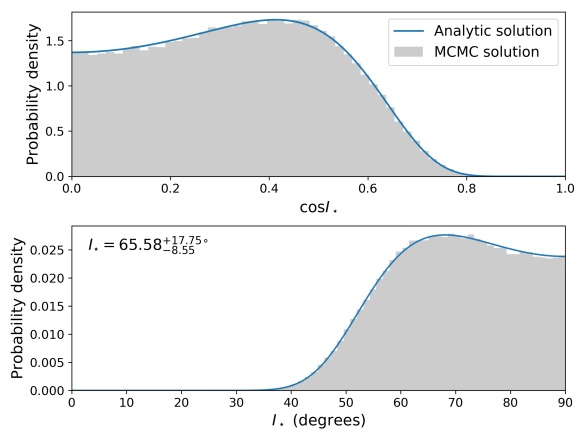
Figure 9: Probability distributions of $\cos{I_{\star}}$ and $I_{\star}$ for TOI-569. The analytic and MCMC solutions follow the procedure outlined by Masuda & Winn (2020).

3.4 Tidal circularization timescales

Over time, tidal interactions between a host star and any companions affect their orbits. Generally, the orbits of the companions and their host stars first begin to circularize according to what is known as the circularization timescale. Next, the orbital period of the companion synchronizes with their host star’s rotation (the synchronization timescale). Finally, the system experiences a spin-orbit co-alignment (Mazeh, 2008). These timescales are influenced by the mass, radius, separation, and tidal quality factor $Q$ of both the host star and companion of a system. Here, we restrict our discussion to the circularization timescales for different values of the tidal quality factors, $Q_{\star}$ and $Q_{\rm BD}$, that may be most appropriate for the TOI-569 and TOI-1406 systems.

Following the formalism from Jackson et al. (2008), the equations for the orbital circularization timescale for a close-in companion are:

$$\frac{1}{\tau_{\rm circ,\star}}=\frac{171}{16}\sqrt{\frac{G}{M_{\star}}}\frac{R_{\star}^{5}M_{\rm BD}}{Q_{\star}}a^{-\frac{13}{2}}$$ (3)

$$\frac{1}{\tau_{\rm circ,BD}}=\frac{63}{4}\frac{\sqrt{GM_{\star}^{3}}R_{\rm BD}^{5}}{Q_{\rm BD}M_{\rm BD}}a^{-\frac{13}{2}}$$ (4)

$$\frac{1}{\tau_{\rm e}}=\frac{1}{\tau_{\rm circ,\star}}+\frac{1}{\tau_{\rm circ,BD}}$$ (5)

Table 6: Circularization timescales for different values of $Q_{\star}$ and $Q_{\rm BD}$ with stellar rotational period and BD orbital period also shown. We quote the rotation period measured from the periodogram of the TESS light curve for TOI-569. An upper limit on the rotation period of TOI-1406 is calculated (Equation 2) using $R_{\star}$ from EXOFASTv2 and FWHM as an approximation for $v\sin{I_{\star}}$. Since we do not directly have the inclination of the star’s rotation axis for TOI-1406, the rotation period listed for this star is an upper limit. The $v\sin{I_{\star}}$ and FWHM values are from CHIRON. These show 1-$\sigma$ uncertainties.

Object name & Age	$Q_{\star}$	$Q_{\rm BD}$	$\tau_{\rm e}$ (Gyr)
TOI-569	$10^{7}$	$10^{6}$	$8.0^{+0.8}_{-1.2}$
$4.70^{+1.30}_{-1.30}$ Gyr	$10^{7}$	$10^{4.5}$	$7.5^{+0.7}_{-1.1}$
	$10^{6}$	$10^{4.5}$	$0.80^{+0.08}_{-0.12}$
	$10^{5}$	$10^{4.5}$	$0.08^{+0.01}_{-0.01}$
TOI-1406	$10^{7}$	$10^{6}$	$127^{+26.2}_{-24.1}$
$3.20^{+2.20}_{-1.60}$ Gyr	$10^{7}$	$10^{4.5}$	$91.5^{+18.4}_{-17.0}$
	$10^{6}$	$10^{4.5}$	$12.4^{+2.5}_{-2.3}$
	$10^{5}$	$10^{4.5}$	$1.3^{+0.3}_{-0.2}$
	$P_{\rm rot}$ (days)	$P_{\rm orb}$ (days)	$v\sin{I_{\star}}$ ($\rm km\,s^{-1}$)
TOI-569	12.9	$6.6$	$5.3\pm 0.5$
	$P_{\rm rot}$ (days)	$P_{\rm orb}$ (days)	$\rm FWHM$ ($\rm km\,s^{-1}$)
TOI-1406	$\leq 5.3$	$10.6$	$12.9\pm 0.2$

where $\tau_{\rm e}$ is the circularization timescale, $a$ is the semi-major axis, $M_{\star}$ is the stellar mass, $R_{\star}$ is the stellar radius, $M_{\rm BD}$ is the BD mass, $R_{\rm BD}$ is the BD radius, $Q_{\star}$ is the tidal quality factor for the star, and $Q_{\rm BD}$ is the tidal quality factor for the BD. Equation 5 is a prediction on how long it takes for the orbital eccentricity of an object to decrease by an exponential factor (the relationship $\tau_{\rm e}\propto dt\propto-de/e$) based on the tides raised on the star and BD.

Use of this equation comes with a number of assumptions that we reiterate here from Jackson et al. (2008): 1) the BD is in a short orbital period (10 days or less), 2) the orbital eccentricity $e$ is small (though for companions in the planetary mass range, higher-order terms may be important to account for higher $e$ in the past), 3) the BD’s orbital period $P_{\rm orb}$ is smaller than the host star’s rotation period $P_{\rm rot}$, and 4) $Q_{\star}$ is independent of the tidal forcing frequency. Admittedly, Equation 5 and these assumptions cater to hot Jupiters and not the type of more massive BDs in this study.

With these considerations in mind, we calculate $\tau_{\rm e}$ for TOI-569b and TOI-1406b for a range of $Q_{\star}$ and $Q_{\rm BD}$ for each system in Table 6. The choice to adopt a $Q_{\rm BD}$ as low as $10^{4.5}$ comes from Beatty et al. (2018), who directly constrain $Q_{\rm BD}$ for CWW 89Ab, a $M_{\rm BD}=39\,{\rm M_{J}}$ BD. The choice to adopt a $Q_{\star}$ as low as $10^{5}$ comes from studies of circularization of binary stars (Meibom & Mathieu, 2005; Milliman et al., 2014). For the bimodal posterior distributions of TOI-569, we only use the most probable $M_{\star}$, $R_{\star}$, $M_{\rm BD}$, $R_{\rm BD}$, and $a$ (Table 9).

We highlight the tidal theory here to show that for these BDs, it is difficult to pin down the timescale over which tidal interactions influence their orbits. Though both BDs have circular orbits, we may only conclude that TOI-1406b likely underwent a low-eccentricity migration unless tidal dissipation was extremely efficient. The circularization timescales for TOI-569 may be short enough such that tidal interactions alone would have circularized the orbit of the BD over the system’s age, thus making it difficult to tell whether or not the BD formed in a circular orbit.

4 Discussion

Including the two new BDs in this work, the total number of known BDs that transit a star is 23 (Table 7). With the discovery of TOI-569b and TOI-1406b, the total number of new transiting BDs discovered or observed by the TESS mission is now 4 (Subjak et al., 2019; Jackman et al., 2019, this work). We expect at least as many more to be discovered as TESS continues its observations over the remainder of its primary mission. At present, we do not have enough transiting BDs to perform a statistical study of the population and draw conclusions about the fundamental origins of BDs and how the mass, radius, and orbital properties of a BD reflects its formation and evolution.

Mass, radius, age, and orbital properties are some of the key aspects that make up a complete understanding of the formation of transiting BDs. Traditionally, astronomers have defined BDs based on their ability to fuse deuterium and their inability to fuse hydrogen. Implicit in this definition is the assumption that BD formation is solely a function of mass. While it may be the case that mass is one of the more important factors in determining whether or not an object is a giant planet, BD, or low-mass star, there is a wealth of evolutionary information to be found in other basic properties.

As we have explored here, the radius, age, and orbital eccentricity give us greater leverage towards understanding transiting BDs. We may combine orbital eccentricity and age with our knowledge of tidal timescales to examine the orbital history of a transiting BD. When the radius and age are used with the mass, we acquire a foothold into the mass-radius diagram for transiting BDs, where we may directly test the accuracy of substellar evolutionary models that seek to explain the underlying physics behind transiting BD formation. In this section, we will look at the population of transiting BDs and discuss how TOI-569b and TOI-1406b fit in to this picture.

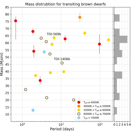
Figure 10: Mass-period distribution of transiting BDs. The colors indicate the effective temperature of the host star of each BD.

4.1 Transiting brown dwarf host star distribution

The mass distribution for the current population of transiting BDs is shown in Figure 10 with the effective temperature of the host star indicated by the colors of the points. From all published studies of transiting BDs to date, there is no obvious preference for a particular type of star to host transiting BDs. Interestingly, we see that 6 transiting BDs (roughly 20% of the transiting BD population, see Table 7) are hosted by an M dwarf star. This is in contrast to hot Jupiters where only a few percent of the hot Jupiter population are found transiting M dwarf stars (e.g. Kepler-45b Johnson et al. (2012), HATS-6b Hartman et al. (2015), WASP-80b Triaud et al. (2015), NGTS-1b Bayliss et al. (2018)). By placing the transiting BD population in the context of eclipsing low-mass stars and hot Jupiters, we may also explore the idea that the scarcity of transiting BDs stems from them spanning the space between the tail ends of the distributions for companions that form like giant planets versus companions that form like low-mass stars. However, more transiting BD discoveries are needed for such studies to yield meaningful results.

4.2 Substellar isochrones and the mass-radius diagram

Here we will discuss how we use transiting BDs with well determined masses, radii, and ages to test the substellar isochrones from Baraffe et al. (2003) (for irradiated BDs) and Saumon & Marley (2008) (for non-irradiated BDs). The Baraffe et al. (2003) models use the same input physics that Chabrier & Baraffe (1997) used for main sequence stars. These are scaled appropriately in Baraffe et al. (2003) for low-mass stars and substellar objects down to $\lessapprox 1\,{\rm M_{J}}$. The way we test these models is by having independent measurements of a transiting BD’s age, which comes from the age of it’s host star (assuming the BD is the same age as its host star). We prioritize the use of stellar ages obtained through studies of clusters, asteroseismology, and gyrochronology, but with Gaia DR2, we are able to reliably determine stellar properties to derive accurate ages with stellar isochrone models such as MIST. This increases the number of transiting BDs for which we have reliable and independently determined ages for comparison to substellar isochrones. This is important because we only know the companion as well as we know the host star and with Gaia DR2, we can now know the host star to greater precision than ever before.

The mass-radius diagram for transiting BDs is shown in Figure 11. All of the BDs on this diagram are necessarily transiting because it is through the transit method that we can measure the radius. However, even though a transit provides some measure of the radius, the measurement is not always very precise (i.e. as precise as the measurement of the stellar radius). This is important because the radius of a BD changes drastically with its age (see Baraffe et al., 2003). Substellar isochrones are challenging to test at ages beyond a few Gyr because the rate at which BD radii contract significantly decelerates, resulting in transiting BD radii approaching an asymptotic limit for the oldest systems (see the differences between the 3-10 Gyr substellar isochrones in Figure 11).

Taking a more critical look at Figure 11, we notice some interesting features. Of the most noticeable are the large ($>10\%$) uncertainties on the radii of no fewer than 6 transiting BDs (AD 3116b, CoRoT-15b, CoRoT-33b, NGTS-7b, NLTT 41135b, and TOI-503b). These are the least informative data points in the substellar mass-radius diagram, especially for objects younger than 1 Gyr as the radius of a transiting BD changes rapidly at ages less than 1 Gyr. Notice also how the substellar isochrone models are mostly horizontal from roughly 20 to 70$\,{\rm M_{J}}$. This means that testing the age of the isochrones is less sensitive to the precision on the mass of a transiting BD than it is to the precision on the radius.

Interestingly, the oldest substellar isochrones are traced fairly well by a handful of transiting BDs. This suggests that the oldest substellar isochrones accurately predict the radii of transiting BDs that approach this asymptotic limit. Future works to improve on the Baraffe et al. (2003) (COND03) and Saumon & Marley (2008) (SM08) models must consider the effects of metallicity for transiting BDs as this may be key to more finely distinguishing the older substellar isochrones from each other, especially in the asymptotic radius regime of 20 to 70$\,{\rm M_{J}}$. The COND03 models do not explore a variety of different metallicity values as the SM08 models do, but the SM08 models do not consider the effects of irradiation like the COND03 models. Additionally, improvements may be made to BDs less massive than $20\,{\rm M_{J}}$ as the input physical prescription from Baraffe et al. (2003) & Chabrier & Baraffe (1997) may not describe these BDs as well as they do more massive objects.

4.2.1 TOI-569b and TOI-1406b in the mass-radius diagram

TOI-569b and TOI-1406b provide us the opportunity to test substellar isochrones older than 2.5 Gyr for the first time because we have accurate masses, radii, and ages traceable to stellar isochrones for their host stars. In this sense, we are using well-tested stellar isochrones to examine relatively untested substellar isochrones.

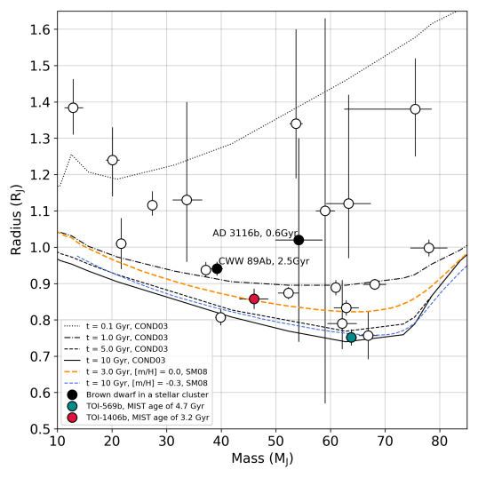
Figure 11: Mass-radius diagram of transiting BDs featuring the COND03 and SM08 models. TOI-569b and TOI-1406b are shown as a cyan point and a red point, respectively. Only 3 BDs that transit main sequence stars have ages constrained by stellar clusters or associations (AD 3116b in Preasepe, CWW 89Ab in Ruprecht 147, and RIK 72b in Upper Scorpius). Note RIK 72b is 5-10 Myr old (David et al., 2019) and is not shown because its radius is $3.1\,{\rm R_{J}}$. Also not shown are the eclipsing BDs in the BD binary system, 2M0535-05, located in the Orion Nebula Cluster with an age of 1-2Myr. Though TOI-569b and TOI-1406b are not in star clusters, we still have relatively precise ages for both from stellar isochrones of their host stars, and in a location on the mass-radius diagram where an age range of 5-10 Gyr results in little change in the models.

Both the COND03 and the SM08 models seem to slightly overestimate the age of TOI-569b to be $\sim$10 Gyr compared to the age of the host star modelled from the MIST isochrones ($4.70\pm 1.30$ Gyr). However, we note that the lower probability bimodal solution for TOI-569b favors a system age of $7.50\pm 1.80$ Gyr, which is in better agreement with the COND03 and SM08 models. The $\log{g}$ of TOI-569 also favors an older system.

Something else worth note is that for a fixed BD mass and age, the radius increases with increasing metallicity (Burrows et al., 2011) and yet, TOI-569b has one of the smallest radii of all known transiting BDs with $\rm[Fe/H]=+0.29$ dex (assuming it matches the host star). When referencing Burrows et al. (2011), Figure 1, we expect a change in the BD’s metallicity ([Fe/H]) from +0.0 dex to +0.5 dex to result as a roughly 0.05-0.1$\,{\rm R_{J}}$ increase in the radius of the BD. There is also an increase of about 0.05$\,{\rm R_{J}}$ when transitioning from clear to cloudy atmospheric models for the BD. This is roughly a factor of two larger than our uncertainties on the radius TOI-569b ($R_{\rm BD}=0.75\pm 0.02\,{\rm R_{J}}$). For TOI-1406, we find that both the COND03 and SM08 models do fairly well at predicting the age of the system ($3.20^{+2.20}_{-1.60}$ Gyr).

4.3 Summary

TOI-569b and TOI-1406b are two newly discovered BDs that transit their host stars in nearly circular orbits. TOI-569 appears to be a slightly evolved G dwarf star with strong photometric modulation interpreted as evolving star spots on the surface of the star. We use the TESS and WASP light curves to extract an estimate for the rotation period of this star to be 13 days and determine that the star’s rotational axis is marginally misaligned with the orbital inclination of TOI-569b. In contrast, TOI-1406 is an F star on the main sequence and with no noticeable photometric modulation over the sectors the star was observed by TESS. By comparing the ages of each system to a range of plausible circularization timescales, we find that we are not able to convincingly determine the orbital history of TOI-569 and that we can at least rule out significant high-eccentricity orbital evolution followed by tidal circularization for TOI-1406.

We demonstrate here how stellar isochrones can be used to test substellar isochrones. This is done by leveraging Gaia DR2 for precise stellar parameters, which translate into better estimates of masses, radii, and ages, of transiting BD.

Ultimately, we find TOI-569b and TOI-1406b to be special in that they contribute new measurements to the still sparsely populated mass-radius diagram for transiting BDs. In addition to providing some of the first examples of a test of the COND03 and SM08 models against stellar isochrones, these systems also offer themselves as new data to examine circularization models. As we build the population of transiting BDs, we will refine the predictive power of substellar isochrones and potentially turn them into tools useful in estimating the ages of transiting BDs.

5 Acknowledgements

Funding for the TESS mission is provided by NASA’s Science Mission directorate. This paper includes data collected by the TESS mission, which are publicly available from the Mikulski Archive for Space Telescopes (MAST). Resources supporting this work were provided by the NASA High-End Computing (HEC) Program through the NASA Advanced Supercomputing (NAS) Division at Ames Research Center for the production of the SPOC data products.

This work has made use of data from the European Space Agency (ESA) mission Gaia (https://www.cosmos.esa.int/gaia), processed by the Gaia Data Processing and Analysis Consortium (DPAC, https://www.cosmos.esa.int/web/gaia/dpac/consortium). Funding for the DPAC has been provided by national institutions, in particular the institutions participating in the Gaia Multilateral Agreement.

TWC acknowledges the efforts of the members of the TESS Followup Program and the Science Processing Operations Center in making the TESS data readily accessible for the analysis in this work.

Funding for this work is provided by the National Science Foundation Graduate Research Fellowship Program Fellowship (GRFP). This work makes use of observations from the LCOGT network.

AJM acknowledges support from the Knut & Alice Wallenberg Foundation (project grant 2014.0017) and the Walter Gyllenberg Foundation of the Royal Physiographical Society in Lund.

CMP and MF gratefully acknowledge the support of the Swedish National Space Agency (DNR 163/16).

AJ and RB acknowledge support by the Ministry for the Economy, Development, and Tourism’s Programa Iniciativa Científica Milenio through grant IC 120009, awarded to the Millennium Institute of Astrophysics (MAS). AJ acknowledges additional support from FONDECYT project 1171208.

All authors especially acknowledge the efforts of the referee and thank them for their thoughtful and constructive feedback on this work.

Table 7: List of published transiting brown dwarfs as of September 2019.

Name	$P$ (days)	$\rm M_{BD}/M_{J}$	$\rm R_{BD}/R_{J}$	e	$\rm M_{\star}/\,{\rm M_{\odot}}$	$\rm R_{\star}/\,{\rm R_{\odot}}$	$\rm T_{eff}(K)$	[Fe/H]	Reference
TOI-569b	6.556	$64.1\pm 1.9$	$0.75\pm 0.02$	$<0.0035$	$1.21\pm 0.05$	$1.47\pm 0.03$	$5768\pm 110$	$+0.29\pm 0.09$	this work
TOI-1406b	10.574	$46.0\pm 2.7$	$0.86\pm 0.03$	$<0.039$	$1.18\pm 0.09$	$1.35\pm 0.03$	$6290\pm 100$	$-0.08\pm 0.09$	this work
HATS-70b	1.888	$12.9\pm 1.8$	$1.38\pm 0.08$	$<0.18$	$1.78\pm 0.12$	$1.88\pm 0.07$	$7930\pm 820$	$+0.04\pm 0.11$	1
KELT-1b	1.218	$27.4\pm 0.9$	$1.12\pm 0.04$	$0.01\pm 0.01$	$1.34\pm 0.06$	$1.47\pm 0.05$	$6516\pm 49$	$+0.05\pm 0.08$	2
NLTT 41135b	2.889	$33.7\pm 2.8$	$1.13\pm 0.27$	$<0.02$	$0.19\pm 0.03$	$0.21\pm 0.02$	$3230\pm 130$	$-0.25\pm 0.25$	3
LHS 6343c	12.713	$62.9\pm 2.3$	$0.83\pm 0.02$	$0.056\pm 0.032$	$0.37\pm 0.01$	$0.38\pm 0.01$	-	$+0.02\pm 0.19$	4
LP 261-75b	1.882	$68.1\pm 2.1$	$0.90\pm 0.02$	$<0.007$	$0.30\pm 0.02$	$0.31\pm 0.01$	$3100\pm 50$	-	5
WASP-30b	4.157	$61.0\pm 0.9$	$0.89\pm 0.02$	0 (adopted)	$1.17\pm 0.03$	$1.30\pm 0.02$	$6201\pm 97$	$-0.08\pm 0.10$	6
WASP-128b	2.209	$37.2\pm 0.9$	$0.94\pm 0.02$	$<0.007$	$1.16\pm 0.04$	$1.15\pm 0.02$	$5950\pm 50$	$+0.01\pm 0.12$	7
CoRoT-3b	4.257	$21.7\pm 1.0$	$1.01\pm 0.07$	0 (adopted)	$1.37\pm 0.09$	$1.56\pm 0.09$	$6740\pm 140$	$-0.02\pm 0.06$	8
CoRoT-15b	3.060	$63.3\pm 4.1$	$1.12\pm 0.30$	0 (adopted)	$1.32\pm 0.12$	$1.46\pm 0.31$	$6350\pm 200$	$+0.10\pm 0.20$	9
CoRoT-33b	5.819	$59.0\pm 1.8$	$1.10\pm 0.53$	$0.070\pm 0.002$	$0.86\pm 0.04$	$0.94\pm 0.14$	$5225\pm 80$	$+0.44\pm 0.10$	10
Kepler-39b	21.087	$20.1\pm 1.3$	$1.24\pm 0.10$	$0.112\pm 0.057$	$1.29\pm 0.07$	$1.40\pm 0.10$	$6350\pm 100$	$+0.10\pm 0.14$	11
KOI-189b	30.360	$78.0\pm 3.4$	$1.00\pm 0.02$	$0.275\pm 0.004$	$0.76\pm 0.05$	$0.73\pm 0.02$	$4952\pm 40$	$-0.07\pm 0.12$	12
KOI-205b	11.720	$39.9\pm 1.0$	$0.81\pm 0.02$	$<0.031$	$0.92\pm 0.03$	$0.84\pm 0.02$	$5237\pm 60$	$+0.14\pm 0.12$	13
KOI-415b	166.788	$62.1\pm 2.7$	$0.79\pm 0.12$	$0.689\pm 0.001$	$0.94\pm 0.06$	$1.15\pm 0.15$	$5810\pm 80$	$-0.24\pm 0.11$	14
EPIC 201702477b	40.737	$66.9\pm 1.7$	$0.76\pm 0.07$	$0.228\pm 0.003$	$0.87\pm 0.03$	$0.90\pm 0.06$	$5517\pm 70$	$-0.16\pm 0.05$	15
EPIC 212036875b	5.170	$52.3\pm 1.9$	$0.87\pm 0.02$	$0.132\pm 0.004$	$1.29\pm 0.07$	$1.50\pm 0.03$	$6238\pm 60$	$+0.01\pm 0.10$	18, 21
AD 3116b	1.983	$54.2\pm 4.3$	$1.02\pm 0.28$	$0.146\pm 0.024$	$0.28\pm 0.02$	$0.29\pm 0.08$	$3200\pm 200$	$+0.16\pm 0.10$	17
CWW 89Ab	5.293	$39.2\pm 1.1$	$0.94\pm 0.02$	$0.189\pm 0.002$	$1.10\pm 0.05$	$1.03\pm 0.02$	$5755\pm 49$	$+0.20\pm 0.09$	16, 18
RIK 72b	97.760	$59.2\pm 6.8$	$3.10\pm 0.31$	$0.146\pm 0.012$	$0.44\pm 0.04$	$0.96\pm 0.10$	$3349\pm 142$	-	19
TOI-503b	3.677	$53.7\pm 1.2$	$1.34^{+0.26}_{-0.15}$	0 (adopted)	$1.80\pm 0.06$	$1.70\pm 0.05$	$7650\pm 160$	$+0.61\pm 0.07$	22
NGTS-7Ab	0.676	$75.5^{+3.0}_{-13.7}$	$1.38^{+0.13}_{-0.14}$	0 (adopted)	$0.48\pm 0.13$	$0.61\pm 0.06$	$3359\pm 106$	-	23
2M0535-05ag	9.779	$56.7\pm 4.8$	$6.50\pm 0.33$	$0.323\pm 0.006$	-	-	-	-	20
2M0535-05bf	9.779	$35.6\pm 2.8$	$5.00\pm 0.25$	$0.323\pm 0.006$	-	-	-	-	20

Note. — References: 1 - Zhou et al. (2019), 2 - Siverd et al. (2012), 3 - Irwin et al. (2010), 4 - Johnson et al. (2011), 5 - Irwin et al. (2018), 6 - Anderson et al. (2011), 7 - Hodžić et al. (2018), 8 - Deleuil et al. (2008), 9 - Bouchy et al. (2011), 10 - Csizmadia et al. (2015), 11 - Bonomo et al. (2015), 12 - Díaz et al. (2014), 13 - Díaz et al. (2013), 14 - Moutou et al. (2013), 15 - Bayliss et al. (2017), 16 - Nowak et al. (2017), 17 - Gillen et al. (2017), 18 - Carmichael et al. (2019), 19 - David et al. (2019), 20 - Stassun et al. (2006), 21 - Persson et al. (2019), 22 - Subjak et al. (2019), 23 - Jackman et al. (2019)

Table 8: MIST median values and 68% confidence interval for TOI-1406, created using EXOFASTv2 commit number 65aa674. Here, $\mathcal{U}$[a,b] is the uniform prior bounded between $a$ and $b$, and $\mathcal{G}[a,b]$ is a Gaussian prior of mean $a$ and width $b$. We show $v\sin{I_{\star}}$ (taken to be the FWHM measured from CHIRON) only for convenient reference; EXOFASTv2 does not model FWHM for spectral line broadening.

Parameter	Units	Priors	Values
Stellar Parameters:
$M_{*}$	Mass ($\,M_{\sun}$)	-	$1.18^{+0.08}_{-0.09}$
$R_{*}$	Radius ($\,R_{\sun}$)	-	$1.35^{+0.03}_{-0.03}$
$L_{*}$	Luminosity ($\,L_{\sun}$)	-	$2.56\pm 0.15$
$\rho_{*}$	Density (cgs)	-	$0.68^{+0.07}_{-0.07}$
$\log{g}$	Surface gravity (cgs)	-	$4.252^{+0.037}_{-0.041}$
$T_{\rm eff}$	Effective Temperature (K)	$\mathcal{G}[6347,186]$	$6290\pm 100$
$[{\rm Fe/H}]$	Metallicity (dex)	$\mathcal{G}[-0.05,0.11]$	$-0.08\pm 0.09$
$Age$	Age (Gyr)	-	$3.20^{+2.20}_{-1.60}$
$EEP$	Equal Evolutionary Point	-	$377^{+40}_{-36}$
$A_{V}$	V-band extinction (mag)	$\mathcal{U}[0,0.08804]$	$0.043^{+0.030}_{-0.029}$
$\sigma_{SED}$	SED photometry error scaling	-	$3.04^{+1.2}_{-0.73}$
$\varpi$	Parallax (mas)	$\mathcal{G}[2.3855,0.0291]$	$2.386\pm 0.029$
$d$	Distance (pc)	-	$419.1^{+5.2}_{-5.0}$
$v\sin{I_{\star}}$	Projected equatorial velocity ($\rm km\,s^{-1}$)	Not modelled	$12.91\pm 0.24$
Brown Dwarf Parameters:
$P$	Period (days)	-	$10.57398^{+0.00060}_{-0.00059}$
$M_{P}$	Mass ($\,{\rm M_{J}}$)	-	$46.0^{+2.6}_{-2.7}$
$R_{P}$	Radius ($\,{\rm R_{J}}$)	-	$0.86\pm 0.03$
$T_{C}$	Time of conjunction ($\rm{BJD_{TDB}}$)	-	$2458414.6065^{+0.0018}_{-0.0019}$
$a$	Semi-major axis (AU)	-	$0.1010^{+0.0022}_{-0.0026}$
$i$	Orbital inclination (Degrees)	-	$87.70^{+0.19}_{-0.20}$
$e$	Eccentricity	-	$0.026^{+0.013}_{-0.010}$
$ecos{\omega_{*}}$		-	$-0.0160^{+0.0079}_{-0.0071}$
$esin{\omega_{*}}$		-	$0.017^{+0.017}_{-0.015}$
$T_{eq}$	Equilibrium temperature (K)	-	$1108^{+18}_{-17}$
$K$	RV semi-amplitude ($\rm m\,s^{-1}$)	-	$3720^{+120}_{-130}$
$logK$	Log of RV semi-amplitude	-	$3.570^{+0.014}_{-0.015}$
$R_{P}/R_{*}$	Radius of planet in stellar radii	-	$0.0654\pm 0.0011$
$a/R_{*}$	Semi-major axis in stellar radii	-	$16.11^{+0.56}_{-0.58}$
$\delta$	Transit depth (fraction)	-	$0.00428\pm 0.00014$
$\tau$	Ingress/egress transit duration (days)	-	$0.0180^{+0.0016}_{-0.0014}$
$b$	Transit Impact parameter	-	$0.648^{+0.033}_{-0.036}$
$\rho_{P}$	Density (cgs)	-	$90^{+11}_{-10.}$
$logg_{P}$	Surface gravity	-	$5.190^{+0.040}_{-0.042}$
$M_{P}\sin i$	Minimum mass ($\,{\rm M_{J}}$)	-	$45.9^{+2.6}_{-2.7}$
$M_{P}/M_{*}$	Mass ratio	-	$0.0372^{+0.0016}_{-0.0015}$
Wavelength Parameters:		TESS band
$u_{1}$	linear limb-darkening coeff	$0.224\pm 0.050$
$u_{2}$	quadratic limb-darkening coeff	$0.299\pm 0.050$
RV Parameters:		ANU	CHIRON
$\gamma_{\rm rel}$	Relative RV Offset ($\rm m\,s^{-1}$)	$-15490^{+200}_{-240}$	$-15461^{+70}_{-68}$
$\sigma_{J}$	RV Jitter ($\rm m\,s^{-1}$)	$380^{+400}_{-260}$	$182^{+85}_{-56}$
$\sigma_{J}^{2}$	RV Jitter Variance	$150000^{+460000}_{-130000}$	$33000^{+38000}_{-17000}$
Transit Parameters:		TESS
$\sigma^{2}$	Added Variance	$-0.000000154^{+0.000000011}_{-0.000000010}$
$F_{0}$	Baseline flux	$0.999996\pm 0.000013$

Table 9: MIST median values and 68% confidence interval for TOI-569, created using EXOFASTv2 commit number 65aa674. The most likely values (probability of 0.73) and the ones we report for this system are shown in boldface. Here, $\mathcal{U}$[a,b] is the uniform prior bounded between $a$ and $b$, and $\mathcal{G}[a,b]$ is a Gaussian prior of mean $a$ and width $b$. We show $v\sin{I_{\star}}$ (measured from CHIRON) only for convenient reference; EXOFASTv2 does not model $v\sin{I_{\star}}$.

Parameter	Units	Priors	Most likely values	Less likely values
Stellar Parameters:			$\rm\bf Prob.=0.73$	$\rm Prob.=0.27$
$M_{*}$	Mass ($\,M_{\sun}$)	-	$\bf 1.21\pm 0.05$	$1.10^{+0.03}_{-0.05}$
$R_{*}$	Radius ($\,R_{\sun}$)	-	$\bf 1.48\pm 0.03$	$1.48\pm 0.03$
$L_{*}$	Luminosity ($\,L_{\sun}$)	-	$\bf 2.15^{+0.15}_{-0.12}$	$2.09\pm 0.1$
$\rho_{*}$	Density (cgs)	-	$\bf 0.54\pm 0.04$	$0.48\pm 0.03$
$\log{g}$	Surface gravity (cgs)	-	$\bf 4.19\pm 0.03$	$4.14\pm 0.02$
$T_{\rm eff}$	Effective Temperature (K)	$\mathcal{G}[5699,106]$	$\bf 5768^{+110}_{-92}$	$5720^{+94}_{-85}$
$[{\rm Fe/H}]$	Metallicity (dex)	$\mathcal{G}[+0.23,0.10]$	$\bf+0.29^{+0.09}_{-0.08}$	$+0.23\pm 0.09$
$Age$	Age (Gyr)	-	$\bf 4.70\pm 1.3$	$7.50^{+1.80}_{-1.20}$
$A_{V}$	V-band extinction (mag)	$\mathcal{U}[0,1.1749]$	$\bf 0.067^{+0.083}_{-0.049}$	$0.052^{+0.074}_{-0.038}$
$\sigma_{SED}$	SED photometry error scaling	-	$\bf 2.99^{+1.10}_{-0.71}$	$3.08^{+1.40}_{-0.78}$
$\varpi$	Parallax (mas)	$\mathcal{G}[6.3723,0.0306]$	$\bf 6.374\pm 0.031$	$6.374^{+0.031}_{-0.030}$
$d$	Distance (pc)	-	$\bf 156.88\pm 0.75$	$156.83\pm 0.75$
$v\sin{I_{\star}}$	Projected equatorial velocity ($\rm km\,s^{-1}$)	Not modelled	$\bf 5.30\pm 0.50$	$5.30\pm 0.50$
Brown Dwarf Parameters:
$P$	Period (days)	-	$\bf 6.55604^{+0.00016}_{-0.00015}$	$6.55603^{+0.00016}_{-0.00015}$
$M_{P}$	Mass ($\,{\rm M_{J}}$)	-	$\bf 64.1^{+1.9}_{-1.4}$	$59.6^{+1.1}_{-1.7}$
$R_{P}$	Radius ($\,{\rm R_{J}}$)	-	$\bf 0.75\pm 0.02$	$0.76\pm 0.02$
$T_{C}$	Time of conjunction ($\rm{BJD_{TDB}}$)	-	$\bf 2458523.09192^{+0.00070}_{-0.00069}$	$2458523.09199\pm 0.00070$
$a$	Semi-major axis (AU)	-	$\bf 0.07428\pm 0.00059$	$0.07207^{+0.00047}_{-0.00069}$
$i$	Orbital inclination (Degrees)	-	$\bf 85.37^{+0.13}_{-0.11}$	$85.15^{+0.13}_{-0.12}$
$e$	Eccentricity	-	$\bf 0.0017^{+0.0018}_{-0.0012}$	$0.0017^{+0.0018}_{-0.0012}$
$ecos{\omega_{*}}$		-	$\bf 0.0002^{+0.0015}_{-0.0011}$	$0.0002^{+0.0015}_{-0.0011}$
$esin{\omega_{*}}$		-	$\bf 0.0005^{+0.0022}_{-0.0012}$	$0.0005^{+0.0022}_{-0.0012}$
$T_{eq}$	Equilibrium temperature (K)	-	$\bf 1227^{+13}_{-12}$	$1237^{+12}_{-13}$
$K$	RV semi-amplitude ($\rm m\,s^{-1}$)	-	$\bf 5884\pm 17$	$5884^{+18}_{-17}$
$logK$	Log of RV semi-amplitude	-	$\bf 3.7697\pm 0.0013$	$3.7697\pm 0.0013$
$R_{P}/R_{*}$	Radius of planet in stellar radii	-	$\bf 0.05217^{+0.00094}_{-0.00091}$	$0.05258^{+0.0010}_{-0.00096}$
$a/R_{*}$	Semi-major axis in stellar radii	-	$\bf 10.81^{+0.22}_{-0.21}$	$10.44^{+0.21}_{-0.20}$
$\delta$	Transit depth (fraction)	-	$\bf 0.002721^{+0.00010}_{-0.000096}$	$0.002765^{+0.00011}_{-0.000100}$
$\tau$	Ingress/egress transit duration (days)	-	$\bf 0.0214^{+0.0015}_{-0.0013}$	$0.0230^{+0.0014}_{-0.0013}$
$b$	Transit Impact parameter	-	$\bf 0.8739^{+0.0082}_{-0.0084}$	$0.8820^{+0.0068}_{-0.0075}$
$\rho_{P}$	Density (cgs)	-	$\bf 187^{+17}_{-16}$	$169^{+16}_{-15}$
$logg_{P}$	Surface gravity	-	$\bf 5.444^{+0.029}_{-0.031}$	$5.412^{+0.027}_{-0.026}$
$M_{P}\sin i$	Minimum mass ($\,{\rm M_{J}}$)	-	$\bf 63.6\pm 1.0$	$59.9^{+0.8}_{-0.9}$
$M_{P}/M_{*}$	Mass ratio	-	$\bf 0.05043^{+0.00097}_{-0.00050}$	$0.05195^{+0.00045}_{-0.00039}$
Wavelength Parameters:		I-band	TESS band
$u_{1}$	linear limb-darkening coeff	$0.292\pm 0.050$	$0.335\pm 0.049$
$u_{2}$	quadratic limb-darkening coeff	$0.260\pm 0.050$	$0.269\pm 0.049$
RV Parameters:		CHIRON	CORALIE	FEROS
$\gamma_{\rm rel}$	Relative RV Offset ($\rm m\,s^{-1}$)	$71964^{+14}_{-16}$	$73413^{+17}_{-18}$	$73402^{+63}_{-55}$
$\sigma_{J}$	RV Jitter ($\rm m\,s^{-1}$)	$37^{+23}_{-17}$	$37^{+27}_{-16}$	$70^{+210}_{-70}$
$\sigma_{J}^{2}$	RV Jitter Variance	$1420^{+2300}_{-1000}$	$1390^{+2800}_{-920}$	$5000^{+76000}_{-7100}$
Transit Parameters:		LCOGT UT 2019-04-15 (I-band)	TESS
$\sigma^{2}$	Added Variance	$0.00000202^{+0.00000030}_{-0.00000026}$	$0.0000001792^{+0.0000000063}_{-0.0000000062}$
$F_{0}$	Baseline flux	$0.99981\pm 0.00013$	$1.0000143\pm 0.0000053$

References

- Anderson et al. (2011) Anderson, D. R., Collier Cameron, A., Hellier, C., et al. 2011, ApJ, 726, L19
- Baraffe et al. (2002) Baraffe, I., Chabrier, G., Allard, F., & Hauschildt, P. H. 2002, A&A, 382, 563
- Baraffe et al. (2003) Baraffe, I., Chabrier, G., Barman, T. S., Allard, F., & Hauschildt, P. H. 2003, A&A, 402, 701
- Barragán et al. (2019a) Barragán, O., Gandolfi, D., & Antoniciello, G. 2019a, MNRAS, 482, 1017
- Barragán et al. (2019b) —. 2019b, MNRAS, 482, 1017
- Bayliss et al. (2017) Bayliss, D., Hojjatpanah, S., Santerne, A., et al. 2017, AJ, 153, 15
- Bayliss et al. (2018) Bayliss, D., Gillen, E., Eigmüller, P., et al. 2018, MNRAS, 475, 4467
- Beatty et al. (2018) Beatty, T. G., Morley, C. V., Curtis, J. L., et al. 2018, AJ, 156, 168
- Bonomo et al. (2015) Bonomo, A. S., Sozzetti, A., Santerne, A., et al. 2015, A&A, 575, A85
- Bouchy et al. (2011) Bouchy, F., Deleuil, M., Guillot, T., et al. 2011, A&A, 525, A68
- Brahm et al. (2017a) Brahm, R., Jordán, A., & Espinoza, N. 2017a, PASP, 129, 034002
- Brahm et al. (2017b) Brahm, R., Jordán, A., Hartman, J., & Bakos, G. 2017b, MNRAS, 467, 971
- Brown et al. (2013) Brown, T. M., Baliber, N., Bianco, F. B., et al. 2013, Publications of the Astronomical Society of the Pacific, 125, 1031
- Burrows et al. (2011) Burrows, A., Heng, K., & Nampaisarn, T. 2011, ApJ, 736, 47
- Carmichael et al. (2019) Carmichael, T., Latham, D., & Vanderburg, A. 2019, The Astronomical Journal, 158, 38. https://doi.org/10.3847%2F1538-3881%2Fab245e
- Castelli & Kurucz (2004) Castelli, F., & Kurucz, R. L. 2004, ArXiv Astrophysics e-prints, astro-ph/0405087
- Chabrier & Baraffe (1997) Chabrier, G., & Baraffe, I. 1997, A&A, 327, 1039
- Choi et al. (2016) Choi, J., Dotter, A., Conroy, C., et al. 2016, ApJ, 823, 102
- Collins et al. (2017) Collins, K. A., Kielkopf, J. F., Stassun, K. G., & Hessman, F. V. 2017, AJ, 153, 77
- Csizmadia & CoRot Team (2016) Csizmadia, S., & CoRot Team. 2016, III.6 Exploration of the brown dwarf regime around solar-like stars by CoRoT, 143
- Csizmadia et al. (2015) Csizmadia, S., Hatzes, A., Gandolfi, D., et al. 2015, A&A, 584, A13
- Cutri & et al. (2013) Cutri, R. M., & et al. 2013, VizieR Online Data Catalog, II/328
- Cutri et al. (2003) Cutri, R. M., Skrutskie, M. F., van Dyk, S., et al. 2003, VizieR Online Data Catalog, II/246
- David et al. (2019) David, T. J., Hillenbrand, L. A., Gillen, E., et al. 2019, ApJ, 872, 161
- Deleuil et al. (2008) Deleuil, M., Deeg, H. J., Alonso, R., et al. 2008, A&A, 491, 889
- Díaz et al. (2013) Díaz, R. F., Damiani, C., Deleuil, M., et al. 2013, A&A, 551, L9
- Díaz et al. (2014) Díaz, R. F., Montagnier, G., Leconte, J., et al. 2014, A&A, 572, A109
- Donati et al. (1997) Donati, J.-F., Semel, M., Carter, B. D., Rees, D. E., & Collier Cameron, A. 1997, MNRAS, 291, 658
- Dotter (2016) Dotter, A. 2016, ApJS, 222, 8
- Eastman et al. (2019) Eastman, J. D., Rodriguez, J. E., Agol, E., et al. 2019, arXiv e-prints, arXiv:1907.09480
- Gaia Collaboration et al. (2018) Gaia Collaboration, Brown, A. G. A., Vallenari, A., et al. 2018, A&A, 616, A1
- Gillen et al. (2017) Gillen, E., Hillenbrand, L. A., David, T. J., et al. 2017, ApJ, 849, 11
- Gray (2005) Gray, D. F. 2005, The Observation and Analysis of Stellar Photospheres
- Hartman et al. (2015) Hartman, J. D., Bayliss, D., Brahm, R., et al. 2015, AJ, 149, 166
- Hodžić et al. (2018) Hodžić, V., Triaud, A. H. M. J., Anderson, D. R., et al. 2018, MNRAS, 481, 5091
- Høg et al. (2000) Høg, E., Fabricius, C., Makarov, V. V., et al. 2000, A&A, 355, L27
- Irwin et al. (2010) Irwin, J., Buchhave, L., Berta, Z. K., et al. 2010, ApJ, 718, 1353
- Irwin et al. (2018) Irwin, J. M., Charbonneau, D., Esquerdo, G. A., et al. 2018, AJ, 156, 140
- Jackman et al. (2019) Jackman, J. A. G., Wheatley, P. J., Bayliss, D., et al. 2019, arXiv e-prints, arXiv:1906.08219
- Jackson et al. (2008) Jackson, B., Greenberg, R., & Barnes, R. 2008, ApJ, 678, 1396
- Jensen (2013) Jensen, E. 2013, Tapir: A web interface for transit/eclipse observability, Astrophysics Source Code Library, , , ascl:1306.007
- Johnson et al. (2011) Johnson, J. A., Apps, K., Gazak, J. Z., et al. 2011, ApJ, 730, 79
- Johnson et al. (2012) Johnson, J. A., Gazak, J. Z., Apps, K., et al. 2012, AJ, 143, 111
- Kaufer & Pasquini (1998) Kaufer, A., & Pasquini, L. 1998, in Proc. SPIE, Vol. 3355, Optical Astronomical Instrumentation, ed. S. D’Odorico, 844–854
- Lightkurve Collaboration et al. (2018) Lightkurve Collaboration, Cardoso, J. V. d. M., Hedges, C., et al. 2018, Lightkurve: Kepler and TESS time series analysis in Python, Astrophysics Source Code Library, , , ascl:1812.013
- Lindegren et al. (2018) Lindegren, L., Hernández, J., Bombrun, A., et al. 2018, A&A, 616, A2
- Mandel & Agol (2002) Mandel, K., & Agol, E. 2002, ApJ, 580, L171
- Marcy & Butler (2000) Marcy, G. W., & Butler, R. P. 2000, PASP, 112, 137
- Masuda & Winn (2020) Masuda, K., & Winn, J. N. 2020, AJ, 159, 81
- Mazeh (2008) Mazeh, T. 2008, in EAS Publications Series, Vol. 29, EAS Publications Series, ed. M. J. Goupil & J. P. Zahn, 1–65
- Meibom & Mathieu (2005) Meibom, S., & Mathieu, R. D. 2005, ApJ, 620, 970
- Milliman et al. (2014) Milliman, K. E., Mathieu, R. D., Geller, A. M., et al. 2014, AJ, 148, 38
- Moutou et al. (2013) Moutou, C., Bonomo, A. S., Bruno, G., et al. 2013, A&A, 558, L6
- Nowak et al. (2017) Nowak, G., Palle, E., Gandolfi, D., et al. 2017, AJ, 153, 131
- Paxton et al. (2015) Paxton, B., Marchant, P., Schwab, J., et al. 2015, ApJS, 220, 15
- Pepe et al. (2002) Pepe, F., Mayor, M., Rupprecht, G., et al. 2002, The Messenger, 110, 9
- Persson et al. (2019) Persson, C. M., Csizmadia, S., Mustill, A. e. J., et al. 2019, A&A, 628, A64
- Queloz et al. (2001) Queloz, D., Mayor, M., Udry, S., et al. 2001, The Messenger, 105, 1
- Quinn & White (2016) Quinn, S. N., & White, R. J. 2016, ApJ, 833, 173
- Saumon & Marley (2008) Saumon, D., & Marley, M. S. 2008, ApJ, 689, 1327
- Siverd et al. (2012) Siverd, R. J., Beatty, T. G., Pepper, J., et al. 2012, ApJ, 761, 123
- Smith et al. (2012) Smith, J. C., Stumpe, M. C., Van Cleve, J. E., et al. 2012, PASP, 124, 1000
- Spiegel et al. (2011) Spiegel, D. S., Burrows, A., & Milsom, J. A. 2011, ApJ, 727, 57
- Stassun et al. (2017) Stassun, K. G., Collins, K. A., & Gaudi, B. S. 2017, AJ, 153, 136
- Stassun et al. (2018a) Stassun, K. G., Corsaro, E., Pepper, J. A., & Gaudi, B. S. 2018a, AJ, 155, 22
- Stassun et al. (2006) Stassun, K. G., Mathieu, R. D., & Valenti, J. A. 2006, Nature, 440, 311
- Stassun & Torres (2016) Stassun, K. G., & Torres, G. 2016, arXiv e-prints, arXiv:1609.05390
- Stassun et al. (2018b) Stassun, K. G., Oelkers, R. J., Pepper, J., et al. 2018b, AJ, 156, 102
- Stumpe et al. (2014) Stumpe, M. C., Smith, J. C., Catanzarite, J. H., et al. 2014, PASP, 126, 100
- Subjak et al. (2019) Subjak, J., Sharma, R., Carmichael, T. W., et al. 2019, arXiv e-prints, arXiv:1909.07984
- Tokovinin (2018) Tokovinin, A. 2018, PASP, 130, 035002
- Tokovinin et al. (2013) Tokovinin, A., Fischer, D. A., Bonati, M., et al. 2013, PASP, 125, 1336
- Triaud et al. (2015) Triaud, A. H. M. J., Gillon, M., Ehrenreich, D., et al. 2015, MNRAS, 450, 2279
- Yee et al. (2017) Yee, S. W., Petigura, E. A., & von Braun, K. 2017, ApJ, 836, 77
- Zhou et al. (2014) Zhou, G., Bayliss, D., Hartman, J. D., et al. 2014, MNRAS, 437, 2831
- Zhou et al. (2019) Zhou, G., Bakos, G. Á., Bayliss, D., et al. 2019, AJ, 157, 31
- Ziegler et al. (2019) Ziegler, C., Tokovinin, A., Briceno, C., et al. 2019, arXiv e-prints, arXiv:1908.10871