First Results on Dark Matter Substructure from Astrometric Weak Lensing

Abstract

Low-mass structures of dark matter (DM) are expected to be entirely devoid of light-emitting regions and baryons. Precisely because of this lack of baryonic feedback, small-scale substructures of the Milky Way are a relatively pristine testing ground for discovering aspects of DM microphysics and primordial fluctuations on subgalactic scales. In this work, we report results from the first search for Galactic DM subhalos with time-domain astrometric weak gravitational lensing. The analysis is based on a matched-filter template of local lensing corrections to the proper motion of stars in the Magellanic Clouds. We describe a data analysis pipeline detailing sample selection, background subtraction, and handling outliers and other systematics. For tentative candidate lenses, we identify a signature based on an anomalous parallax template that can unequivocally confirm the presence of a DM lens, opening up prospects for robust discovery potential with full time-series data. We present our constraints on substructure fraction $f_{l}\lesssim 5$ at 90% CL (and $f_{l}\lesssim 2$ at 50% CL) for compact lenses with radii $r_{l}<1\,\mathrm{pc}$, with best sensitivity reached for lens masses $M_{l}$ around $10^{7}$–$10^{8}\,M_{\odot}$. Parametric improvements are expected with future astrometric data sets; by end of mission, Gaia could reach $f_{l}\lesssim 10^{-3}$ for these massive point-like objects, and be sensitive to lighter and/or more extended subhalos for $\mathcal{O}(1)$ substructure fractions.

I Introduction

The precise nature of the constituents of the dark matter (DM) and their microphysical properties is not known. Nevertheless, a wealth of information has been collected about its macroscopic properties and behavior from its minimal coupling to gravity and its resulting gravitational influence. In the linear theory of structure formation, a fluid with adiabatic fluctuations and vanishing sound speed clusters in a way that shows remarkable agreement with observations of the cosmic microwave background Ade et al. (2016a); Aghanim et al. (2018), the Lyman-$\alpha$ forest Seljak et al. (2006); Blomqvist et al. (2019); Agathe et al. (2019), and large-scale structures Percival and White (2009); Howlett et al. (2015); Zarrouk et al. (2018). This evolution has been probed over comoving length scales between $0.1\,\mathrm{Mpc}$ and $10^{4}\,\mathrm{Mpc}$ starting from a time when the Universe and the DM were more than 10 orders of magnitude denser than at the present time. N-body simulations Springel et al. (2008); Diemand et al. (2008); Boylan-Kolchin et al. (2009); Stadel et al. (2009); Garrison-Kimmel et al. (2014); Vogelsberger et al. (2014); Hellwing et al. (2016) extend these predictions to smaller physical length scales and into the nonlinear regime, matching observations of galactic rotation curves Rubin and Ford Jr (1970); Freeman (1970); Rogstad and Shostak (1972); Whitehurst and Roberts (1972); Roberts and Rots (1973), statistical dispersion relations Zwicky (1933); Smith (1936); Zwicky (1937); Girardi et al. (1998); Rines and Diaferio (2006); Becker et al. (2007), weak Kaiser and Squires (1993); Schneider (1996); Wittman et al. (2000); Hoekstra et al. (2004); Okabe et al. (2014) and strong Keeton (2001); Treu (2010); Jullo et al. (2010) gravitational lensing, and the distribution and abundance of satellite galaxies Klypin et al. (1999); Willman et al. (2004); Tollerud et al. (2008). These complementary bodies of evidence not only put the existence of DM on a strong footing, they also provide knowledge about its coarse-grained phase-space distribution, indispensable input to searches for any nonminimal DM couplings.

Detection of smaller DM structures becomes increasingly challenging due to their lower light-to-mass ratios; DM halos with scale masses below $10^{8}\,M_{\odot}$ do not harbor conditions for star formation and are thus entirely dark Rees and Ostriker (1977); Kravtsov (2010); Bromm (2013). Methods reliant on the minimal coupling to gravity include fluctuations in extragalactic strong gravitational lenses Mao and Schneider (1998); Metcalf and Madau (2001); Chiba (2002); Dalal and Kochanek (2002); Metcalf and Zhao (2002); Koopmans et al. (2002); Kochanek and Dalal (2004); Inoue and Chiba (2005a, b); Koopmans (2005); Chen et al. (2007); Williams et al. (2008); More et al. (2009); Keeton and Moustakas (2009); Vegetti and Koopmans (2009a, b); Congdon et al. (2010); Hezaveh et al. (2013); Vegetti and Vogelsberger (2014); Hezaveh et al. (2016a, b), stellar wakes in the MW disk Feldmann and Spolyar (2014) and halo Buschmann et al. (2017), diffraction of gravitational waves Dai et al. (2018), photometric irregularities of micro-caustic light curves Dai and Miralda-Escudé (2019), and perturbations of cold stellar streams Ibata et al. (2002); Johnston et al. (2002); Siegal-Gaskins and Valluri (2008); Bovy (2016); Carlberg (2016); Erkal et al. (2016); Bonaca and Hogg (2018) (with tentative positive detections Bonaca et al. (2018); Banik et al. (2019)). These techniques show significant promise but are indirect or applicable to extragalactic structures only. Direct searches for MW substructure have so far been confined to transients in photometric lensing Paczynski (1986); Alcock et al. (2000); Tisserand et al. (2007); Griest et al. (2014); Niikura et al. (2017); Zumalacarregui and Seljak (2018) and pulsar timing Siegel et al. (2007); Seto and Cooray (2007); Baghram et al. (2011); Kashiyama and Seto (2012); Clark et al. (2015); Schutz and Liu (2017); Dror et al. (2019), which only produce detectable signals for ultracompact objects such as black holes but not for more extended structures such as DM halos that collapse after matter-radiation equality.

In this Letter, we present the first results of a qualitatively new class of searches for Galactic DM substructure using time-domain, astrometric, weak gravitational lensing. Ref. Van Tilburg et al. (2018) proposed several categories of observables to this effect, and forecasted their sensitivity on upcoming astrometric surveys. We employ a refined version of their “local velocity template” on a sample of Small and Large Magellanic Cloud (SMC and LMC) stars in Gaia’s second data release (DR2). Our data analysis constitutes a robust, optimal, matched-filter-based search for local distortions of the proper motion field of background sources produced by the gravitational lensing of intervening foreground compact DM subhalos. We find no evidence of this effect, setting a constraint of $f_{l}\equiv\Omega_{l}/\Omega_{\mathrm{DM}}\lesssim 5$ at 90% CL (and $f_{l}\lesssim 2$ at 50 % CL) for $M_{l}\sim 10^{8}\,M_{\odot}$ and $r_{l}\lesssim 1\,\mathrm{pc}$, where $f_{l}$ is the DM substructure fraction, and $M_{l}$ and $r_{l}$ are the mass and characteristic radius of the subhalos. Currently limited by statistical instrumental uncertainties, we expect the reach to the combination $f_{l}M_{l}^{2}/r_{l}^{3}$ to improve as $\propto t_{\mathrm{int}}^{-9/2}$, with the integration time $t_{\mathrm{int}}$ set to increase fivefold by Gaia’s end of mission.

A localized discovery of dark low-mass substructures with our technique, possible with future astrometric surveys, would be a watershed event. Because of the absence of baryonic feedback, their abundance, mass function, and density profiles would provide a transparent window on the primordial fluctuation spectrum and the DM’s transfer function on comoving scales below $0.1\,\mathrm{Mpc}$. It would probe the spectrum of adiabatic perturbations produced from the inflationary stage after the one measured in the CMB Ade et al. (2016b); Akrami et al. (2018) and the Ly-$\alpha$ forest Bird et al. (2011), and of small-scale isocurvature fluctuations produced from e.g. a late phase transition in the DM sector Zurek et al. (2007); Buschmann et al. (2019). Their discovery (non-observation) would rule out (provide evidence for) small-scale structure suppression, unavoidable predictions of light fermion (“warm”) Colin et al. (2000); Bode et al. (2001); Viel et al. (2005) and ultralight scalar (“fuzzy”) Hu et al. (2000); Li et al. (2014); Hui et al. (2017) DM models. Enhanced-density subhalos can result from dissipation and self-interactions in the DM sector Agrawal and Randall (2017); Chang et al. (2019); Essig et al. (2019), or early-time structure growth in axion DM models with large misalignment Arvanitaki et al. (2019).

II Lensing signal

The physical effect under consideration is time-domain weak gravitational lensing of the astrometric kind, summarized in Fig. 1. “Weak” refers to the regime where the impact parameter is much larger than the Einstein radius of the lens and one image of the source is resolved by the observer, and “astrometric” refers to the effect of angular deflection of the source’s light centroid. True celestial positions $\bm{\mathbf{\theta}}_{i}$ are unknown a priori, rendering the angular deflection $\Delta\bm{\mathbf{\theta}}_{il}$ of source $i$ by lens $l$ unobservable in practice.

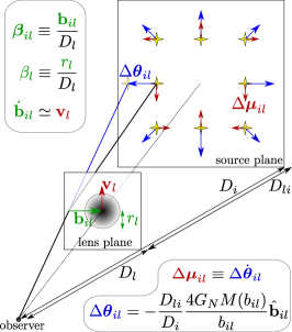
Figure 1: Diagram of gravitational lensing geometry of sources $i$ by a lens $l$. The impact parameter is $\bm{\mathbf{b}}_{il}$, its rate of change $\bm{\mathbf{v}}_{l}$, the lens radius $r_{l}$, and respective line-of-sight distances $D_{i,l}$. In celestial coordinates, the angular impact parameter is $\bm{\mathbf{\beta}}_{il}\equiv\bm{\mathbf{\theta}}_{i}-\bm{\mathbf{\theta}}_{l}$, angular lens radius $\beta_{l}$. The angular displacement $\Delta\bm{\mathbf{\theta}}_{il}$ (blue, monopole pattern) is not constant in time, leading to lensing corrections $\Delta\bm{\mathbf{\mu}}_{il}$ to the sources’ proper motions $\bm{\mathbf{\mu}}_{i}$ (red, dipole pattern).

Ref. Van Tilburg et al. (2018) proposed leveraging time-domain lensing effects due to the relative rate of change in impact parameter $\dot{\bm{\mathbf{b}}}_{il}\simeq\bm{\mathbf{v}}_{l}$ in the reference frame of the observer. (We ignore the small contribution of the distant background source motions to $\dot{\bm{\mathbf{b}}}_{il}$.) The leading observable in the time-domain (i.e. to first order in $\bm{\mathbf{v}}_{l}$) is a lensing correction to the proper motion $\bm{\mathbf{\mu}}_{i}$:

$$\Delta\bm{\mathbf{\mu}}_{il}\equiv\Delta\dot{\bm{\mathbf{\theta}}}_{il}=\frac{D_{il}}{D_{i}}\frac{4G_{N}M_{l}v_{l}}{r_{l}^{2}}\tilde{\bm{\mathbf{\mu}}}_{i}(\beta_{l},\bm{\mathbf{\beta}}_{il},\hat{\bm{\mathbf{v}}}_{l}),$$ (1)

where $G_{N}$ is Newton’s gravitational constant, $r_{l}$ a characteristic lens radius, and $M_{l}=4\pi\int_{0}^{\infty}{\rm d}r\,r^{2}\,\rho_{l}(r)$ the mass of the lens with 3D density profile $\rho_{l}(r)$. The unit-less 2D spatial profile of the distortion is

$$\tilde{\bm{\mathbf{\mu}}}_{i}(\beta_{l},\bm{\mathbf{\beta}}_{il},\hat{\bm{\mathbf{v}}}_{l}) =\frac{\widetilde{M}_{l}(\beta_{il})}{\beta_{il}^{2}/\beta_{l}^{2}}\left[2\hat{\bm{\mathbf{\beta}}}_{il}(\hat{\bm{\mathbf{\beta}}}_{il}\cdot\hat{\bm{\mathbf{v}}}_{l})-\hat{\bm{\mathbf{v}}}_{l}\right]$$

$$\phantom{=}-\frac{\partial_{\beta_{il}}\widetilde{M}(\beta_{il})}{\beta_{il}/\beta_{l}^{2}}\hat{\bm{\mathbf{\beta}}}_{il}(\hat{\bm{\mathbf{\beta}}}_{il}\cdot\hat{\bm{\mathbf{v}}}_{l})$$ (2)

with $M(b)=2\pi\int_{-\infty}^{\infty}{\rm d}z\,\int_{0}^{b}{\rm d}b^{\prime}\,b^{\prime}\rho_{l}(\sqrt{z^{2}+b^{\prime 2}})$ the enclosed lens mass within a cylinder oriented along the line of sight ($z$-direction) with radius equal to $b$, cfr. Fig. 1, and $\widetilde{M}(\beta_{il})\equiv M(b_{il})/M_{l}$. We also introduced the lens angular size $\beta_{l}\equiv r_{l}/D_{l}$ and angular impact parameter $\bm{\mathbf{\beta}}_{il}\equiv\bm{\mathbf{b}}_{il}/D_{l}$.

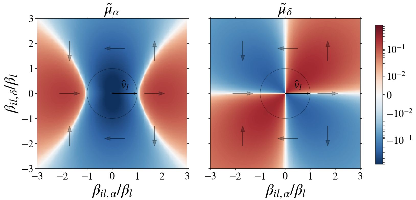
Figure 2: Right-ascension ($\alpha$, left) and declination ($\delta$, right) components of the angular velocity vector profile $\tilde{\bm{\mathbf{\mu}}}_{i}$ of Eq. 2 as a function of angular separation $\bm{\mathbf{\beta}}_{il}$ for the lens density profile of Eq. 3. The lens has angular size $\beta_{l}$ and is moving in the direction $\hat{\bm{\mathbf{v}}}_{l}=\hat{\bm{\mathbf{v}}}_{\alpha}$.

The primary lensing signature is thus a distortion in the angular velocity of background sources with a magnitude given by the prefactor in Eq. 1 and the characteristic spatial pattern of Eq. 2, which is a universal dipole pattern for sources far outside the lens radius $\beta_{il}/\beta_{l}$ and depends on the lens density profile for sources eclipsed by the lens. For specificity, we will assume a lens density profile of

$$\rho_{l}(r)=\frac{M_{l}}{4\pi}\frac{\exp\{-\frac{r^{2}}{2r_{l}^{2}}\}}{rr_{l}^{2}}$$ (3)

throughout the main text. The above profile exhibits the $1/r$ cusp of the NFW profile, but is nearly optimal in that it has no significant mass outside the scale radius (the radius where $\partial_{\ln r}(\ln\rho_{l})=-2$, in this case $r=r_{l}$), which would contribute to the lens mass abundance but only minimally to the lensing signal. The analysis presented here can easily be adapted to other density profiles, such as a pure Gaussian or a tidally truncated NFW profile, by properly choosing the function $\widetilde{M}_{l}$ in Eq. 2. In the Appendix, we will investigate a profile-agnostic approach by truncating the lensing signal at $r_{l}$. In Fig. 2, we display the angular velocity distortion pattern of Eq. 2 resulting from the density profile in Eq. 3.

We take the lenses’ spatial distribution across the Milky Way to follow that of the Galactic DM halo with a fiducial NFW profile

$$\rho(\bm{\mathbf{r}})=\frac{4\rho_{s}}{\frac{r}{R_{s}}\big{[}1+\frac{r}{R_{s}}\big{]}^{2}},\;R_{s}=18\,\mathrm{kpc},\;\rho_{s}=0.003\,\frac{\mathrm{M_{\odot}}}{\mathrm{pc}^{3}},$$ (4)

with $r$ the galactocentric radius, and the observer located at $r_{\odot}=8\,\mathrm{kpc}$ McMillan (2011). We assume a transverse lens velocity distribution for the subhalos given by:

$$p_{v}(\bm{\mathbf{v}}_{l})=\frac{1}{2\pi\sigma_{v}^{2}}\exp\left[-\frac{\left(\bm{\mathbf{v}}_{l}-\bm{\mathbf{v}}_{0}\right)^{2}}{2\sigma_{v}^{2}}\right],\;\sigma_{v}\simeq 166\,\frac{\mathrm{km}}{\mathrm{s}},$$ (5)

where $\bm{\mathbf{v}}_{0}$ denotes a 2D velocity vector equal in magnitude and opposite to the observer’s velocity projected on the plane perpendicular to the line of sight. We take the observer’s velocity to be the Solar System velocity of $238$ km/s in the Galactic equatorial plane ($b\approx 0$, $l\approx 270^{\circ}$). In the following, we will ignore the additional annual rotation around the Sun, but will return to this parallax effect in the Discussion.

III Template method

We utilize a local test statistic $\mathcal{T}$ that computes the overlap of the velocity field of background sources with the one induced by a tentative lens candidate with angular position $\bm{\mathbf{\theta}}_{t}$, angular scale $\beta_{t}$, and effective lens velocity direction $\hat{\bm{\mathbf{v}}}_{t}$ Van Tilburg et al. (2018):

$$\mathcal{T}(\bm{\mathbf{\theta}}_{t},\beta_{t},\hat{\bm{\mathbf{v}}}_{t}) \equiv\sum_{i}\frac{\bm{\mathbf{\mu}}_{i}\cdot\tilde{\bm{\mathbf{\mu}}}_{i}(\beta_{t},\bm{\mathbf{\beta}}_{it},\hat{\bm{\mathbf{v}}}_{t})}{\sigma_{\mu,i}^{2}},$$ (6)

where $\bm{\mathbf{\mu}}_{i}\equiv\{\mu_{i,\alpha*},\mu_{i,\delta}\}=\{\mu_{i,\alpha}\cos{\delta_{i}},\mu_{i,\delta}\}$ is the proper motion vector of the $i$th star, and $\sigma_{\mu,i}^{2}\equiv\sigma_{\mu_{\alpha},i}^{2}+\sigma_{\mu_{\delta},i}^{2}$ is the measured variance over the chosen stellar population. The velocity template vector $\tilde{\bm{\mathbf{\mu}}}_{i}$ is a matched filter to the lens-induced velocity vector profile and is given in Eq. 2 generally, and for the specific density profile of Eq. 3 in Fig. 2. $\mathcal{T}$ depends on the lens position through the angular impact parameters $\bm{\mathbf{\beta}}_{it}\equiv\bm{\mathbf{\theta}}_{t}-\bm{\mathbf{\theta}}_{i}$.

We define the normalization factor

$$\mathcal{N}^{2}(\bm{\mathbf{\theta}}_{t},\beta_{t}) \equiv\sum_{i}\frac{|\tilde{\bm{\mathbf{\mu}}}_{i}(\beta_{t},\bm{\mathbf{\beta}}_{it},\hat{\bm{\mathbf{v}}}_{t})|^{2}}{\sigma_{\mu,i}^{2}},$$ (7)

that acts as a figure of merit for the sensitivity of a candidate lens position and radius: large values indicate the presence of numerous low-noise stars within $\beta_{t}$ around the template. In absence of a lensing signal, one expects vanishing mean $\langle\mathcal{T}\rangle_{\mathrm{n}}$ with a variance $\langle\mathcal{T}^{2}\rangle_{\mathrm{n}}=\mathcal{N}^{2}\sim\Sigma\beta_{t}^{2}/\sigma_{\mu}^{2}$ with $\Sigma$ the typical local angular number density of background sources.

In the presence of a lens, and with template parameters perfectly matched to those of the lens (i.e. $\bm{\mathbf{\theta}}_{t}=\bm{\mathbf{\theta}}_{l}$, $\beta_{t}=\beta_{l}$, and $\hat{\bm{\mathbf{v}}}_{t}=\hat{\bm{\mathbf{v}}}_{l}$), the test statistic is expected to evaluate to $\langle\mathcal{T}\rangle_{\mathrm{s}}\simeq\mathcal{N}^{2}4G_{N}M_{l}v_{l}/r_{l}^{2}$ for a nearby lens $D_{l}\ll D_{i}$. The local signal-to-noise ratio

$$\mathrm{SNR}=\frac{\langle\mathcal{T}\rangle_{\mathrm{s}}}{\sqrt{\langle\mathcal{T}^{2}\rangle_{\mathrm{n}}}}\simeq\frac{4G_{N}M_{l}v_{l}}{r_{l}^{2}}\mathcal{N}\sim\frac{4G_{N}M_{l}v_{l}\sqrt{\Sigma}}{r_{l}D_{l}\sigma_{\mu}}$$ (8)

is generally largest for the most nearby, massive, compact, and fast-moving lenses in front of high-density, low-noise regions.

The true lens properties are unknown a priori. We evaluate $\mathcal{T}$ over a dense grid in $\bm{\mathbf{\theta}}_{t}$ and $\beta_{t}$, and for two lens velocity directions (along RA and DEC) $\mathcal{T}_{\alpha}(\bm{\mathbf{\theta}}_{t},\beta_{t})\equiv\mathcal{T}(\bm{\mathbf{\theta}}_{t},\beta_{t},\hat{\bm{\mathbf{\alpha}}})$ and similarly for $\mathcal{T}_{\delta}$ which we will combine into a vector $\bm{\mathbf{\mathcal{T}}}\equiv\{\mathcal{T}_{\alpha},\mathcal{T}_{\delta}\}$. The directional asymmetry in Eq. 5 translates into the same preferred direction for the template $\langle\bm{\mathbf{\mathcal{T}}}\rangle_{\mathrm{s}}\propto\bm{\mathbf{v}}_{0}$.

We define a global test statistic $\mathcal{R}$ that is the optimal observable (see Appendix for derivation) for detecting the proper motion distortion of a single lens across a certain patch of sky:

$$\mathcal{R}=\sup_{\bm{\mathbf{\theta}}_{t},\beta_{t}}\Bigg{[}\ln\frac{\rho}{\beta_{t}^{4}}+\frac{C^{2}\sigma_{v}^{2}\mathcal{N}^{2}\Big{(}\frac{\mathcal{T}^{2}}{\mathcal{N}^{2}}-\frac{v_{0}^{2}}{\sigma_{v}^{2}}\Big{)}+2C\bm{\mathbf{\mathcal{T}}}\cdot\bm{\mathbf{v}}_{0}}{2(1+C^{2}\sigma_{v}^{2}\mathcal{N}^{2})}\Bigg{]}$$ (9)

with $\rho=\rho(\bm{\mathbf{\theta}}_{t},r_{l}/\beta_{t})$ from Eq. 4, $C=4G_{N}M_{l}/r_{l}^{2}$ and $\mathcal{T}^{2}=\mathcal{T}_{\alpha}^{2}+\mathcal{T}_{\delta}^{2}$. Roughly speaking, it corresponds to taking the largest value of $\bm{\mathbf{\mathcal{T}}}/\mathcal{N}$ across the densely-scanned grid of $\{\bm{\mathbf{\theta}}_{t},\beta_{t}\}$, but it also properly accounts for the $\bm{\mathbf{v}}_{l}$ asymmetry, variations in $\mathcal{N}(\theta_{t},\beta_{t})$, and priors on the 3D location of the lens.

IV Data Processing

Data sample—

For our analysis, we choose astrometric data on the Large and Small Magellanic Clouds (LMC and SMC) from Gaia’s second data release Prusti et al. (2016); Brown et al. (2018). They have large stellar angular number densities and low proper motion dispersion (intrinsic and instrumental), maximizing the SNR of Eq. 8 with a high $\sqrt{\Sigma}/\sigma_{\mu}$. Their large combined angular area also increases the probability of at least one nearby (low $D_{l}$) lens.

To avoid foreground contamination, we select sources without evidence of parallax ($\varpi$ /$\sigma_{\varpi}<2$) in a square of $10^{\circ}$ sidelength centered on $(\alpha,\delta)=(78.77^{\circ},-69.01^{\circ})$ for the LMC and $8^{\circ}$ on $(12.80^{\circ},-73.15^{\circ})$ for the SMC. For the SMC, we impose $|\mu_{\alpha*}-0.685\,\mathrm{mas/y}|<2\,\mathrm{mas/y}$ and $|\mu_{\delta}+1.230\,\mathrm{mas/y}|<2\,\mathrm{mas/y}$ to cut out the foreground NGC 104 and NGC 362 globular clusters. Poor astrometric solutions were avoided with a cut on Renormalized Unit Weight Error of $\mathrm{RUWE}<1.4$ Lindegren (2018). We summarize our data processing operations here and refer the interested reader to the Appendix for more details.

Removal of dense clusters—

Overdense stellar clusters generally move coherently and independently from the bulk stars in the Magellanic Clouds (MCs), and are thus contaminants from our perspective. We calculate a smoothed angular number density map $\Sigma_{\mathrm{sm}}(\bm{\mathbf{\theta}})$ with a Gaussian kernel of angular radius $0.1^{\circ}$ and a pixelated angular number density map $\Sigma(\bm{\mathbf{\theta}})$ with pixels of size $0.1^{\circ}/3$. Density outliers are removed by excising regions for which $\Sigma>3\Sigma_{\mathrm{sm}}$.

Motion subtraction and outlier removal—

We subtract the large-scale proper motion and remove stars that are not bound to the MCs. Operationally, we define a motion field $\bm{\mathbf{\mu}}(\bm{\mathbf{\theta}}_{p})=\sum_{i\in p}\bm{\mathbf{\mu}}_{i}\sigma_{\mu,i}^{-2}/\sum_{i\in p}\sigma_{\mu,i}^{-2}$ in square pixels $p$ of $0.05^{\circ}$, from which we calculate a smoothed motion field $\bm{\mathbf{\mu}}_{\mathrm{sm}}(\bm{\mathbf{\theta}})$ with Gaussian kernel of radius $0.1^{\circ}$. We then construct a list of stellar motions with large-scale motion subtracted: $\bm{\mathbf{\mu}}_{\mathrm{sub},i}\equiv\bm{\mathbf{\mu}}_{i}-\bm{\mathbf{\mu}}_{\mathrm{sm}}(\bm{\mathbf{\theta}}_{i})$. Stars with $\mu_{\mathrm{sub},i}>3\sigma_{\mu,i}+\mu_{\mathrm{esc}}$ are removed, were $\mu_{\mathrm{esc}}$ is the (proper) escape velocity. The outlier removal slightly biases $\bm{\mathbf{\mu}}_{\mathrm{sm}}$, so the process is iterated another two times with the remaining stars.

Effective error—

After the above procedures, we arrive at a proper motion field with $\langle\bm{\mathbf{\mu}}_{\mathrm{sub},i}\rangle\simeq 0$ but where the observed variance $\sigma_{\mu,\mathrm{eff}}^{2}\equiv\langle\mu_{\mathrm{sub},i}^{2}\rangle$ still exceeds the Gaia-reported variance $\sigma_{\mu,\mathrm{Gaia}}^{2}\equiv\langle\sigma_{\mu,i}^{2}\rangle$. This discrepancy is due to intrinsic (proper) velocity dispersion $\sigma_{\mu,\mathrm{intrinsic}}$ in the MCs as well as unmodeled instrumental systematics, unresolved binaries and double stars, and other astrometric misfits Arenou et al. (2018); Lindegren et al. (2018). In Fig. 3, we plot the number of stars (red), $\sigma_{\mu,\mathrm{eff}}$ (blue), $\sigma_{\mu,\mathrm{Gaia}}$ (green), and $\sigma_{\mu,\mathrm{intrinsic}}$ (gray) Gyuk et al. (2000); Evans and Howarth (2008) in bins of 0.1 width in G magnitude for the LMC (thick) and SMC (thin). In the following analysis, we use the G-mag-dependent $\sigma_{\mu,\mathrm{eff}}^{2}$ as the inverse weight factor in Eqs. 6 and 7.

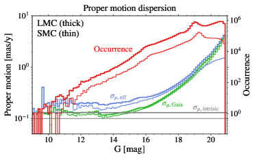
Figure 3: Number of stars (red), observed ($\sigma_{\mu,\text{eff}}$, blue), reported ($\sigma_{\mu,\textit{Gaia}}$, green), and intrinsic ($\sigma_{\mu,\text{intrinsic}}$, gray) proper motion dispersion as a function of stellar G magnitude for the LMC (thick) and SMC (thin).

V Analysis & Results

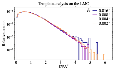
Figure 4: Histograms of the local test statistic $\mathcal{T}(\bm{\mathbf{\theta}}_{t},\beta_{t})/\mathcal{N}(\bm{\mathbf{\theta}}_{t},\beta_{t})$, where $\mathcal{T}=\sqrt{\mathcal{T}_{\alpha}^{2}+\mathcal{T}_{\delta}^{2}}$, evaluated at all template locations $\bm{\mathbf{\theta}}_{t}$ and different angular template radii $\beta_{t}$ for the coarse-grid analysis on the LMC data sample.

Evaluation of test statistics—

We compute $\bm{\mathbf{\mathcal{T}}}(\bm{\mathbf{\theta}}_{t},\beta_{t})$ and $\mathcal{N}(\bm{\mathbf{\theta}}_{t},\beta_{t})$ over a coarse square grid with lattice constant $\beta_{\mathrm{scan}}=0.9\times\beta_{t}$ for a fixed list of 58 $\beta_{t}$ values evenly spaced between $0.0015^{\circ}$ and $0.03^{\circ}$. The results of this procedure for 4 angular scales are displayed for the LMC data in Fig. 4, and exhibit a near-Gaussian distribution of $\mathcal{T}/\mathcal{N}$ out to $5$ sigma. At each $\beta_{t}$, we then identify coarse lattice sites at which $\mathcal{T}>0.25\max_{\bm{\mathbf{\theta_{t}}}}\mathcal{T}$, and compute $\bm{\mathbf{\mathcal{T}}},\mathcal{N}$ over sets of finer grids with lattice constant $\beta^{\prime}_{\mathrm{scan}}=\beta_{\mathrm{scan}}/3$ around these high-$\mathcal{T}$ sites. This finer scanning procedure is iterated once more with $\beta^{\prime\prime}_{\mathrm{scan}}=\beta^{\prime}_{\mathrm{scan}}/3$ at lattice sites at which $\mathcal{T}>0.5\max_{\bm{\mathbf{\theta_{t}}}}\mathcal{T}$. For each parameter space point in the 3D space $\{M_{l},r_{l},f_{l}\}$, we calculate $\mathcal{R}$ as defined in Eq. 9 from the finest grid of $\bm{\mathbf{\mathcal{T}}},\mathcal{N}$ values over the combined LMC/SMC sample.

Signal simulations—

For each point in $\{M_{l},r_{l},f_{l}\}$, we create a minimum of 100 simulations of lensing signal and stochastic noise. In each simulation, we generate a random number $N_{l}$ of lenses from a Poisson distribution with mean $\langle N_{l}\rangle=\Delta\Theta\ (\Omega_{l}/M_{l})\int_{0}^{D_{i}}{\rm d}D_{l}\,D_{l}^{2}\rho(\bm{\mathbf{\theta}}_{i},D_{l})$ with $\rho(\bm{\mathbf{r}})$ from Eq. 4 and $\Delta\Theta$ the solid angle subtended by the data, for both the LMC and SMC. The pdf for the 3D position of the lenses $(D_{l},\bm{\mathbf{\theta}}_{l})$ (determining $\beta_{l}$) is taken proportional to $\rho(\bm{\mathbf{r}})$, and that for $\bm{\mathbf{v}}_{l}$ is given by Eq. 5.

In each of the simulations, we inject stochastic proper motion noise. We first group the stars in two-dimensional bins of $0.05$ width in G magnitude and $1^{\circ}$ radial bins from the centers of the LMC and SMC, and then deduce the proper motion pdf by equating it to the observed distribution of $\bm{\mathbf{\mu}}_{\mathrm{sub},i}$ in each bin on the data samples. (These pdfs are decidedly non-Gaussian, only the variance of their 1D G-mag projection is shown in Fig. 3). Finally, we produce signal-plus-noise simulations by random draws from these proper motion noise pdfs, and by subsequent distortions via Eq. 1 from their associated random lens population.

Constraints—

The simulations are run through the exact same data processing and analysis pipeline (in particular also the motion subtraction and outlier removal) as the actual data, yielding a distribution of $\mathcal{R}$ values for each parameter space point in $\{M_{l},r_{l},f_{l}\}$. If 90% (50%) of the simulations have an $\mathcal{R}$ value larger than the observed $\mathcal{R}$ value for any parameter space point, then that point is excluded at 90% (50%) CL. As a cross-check on our limit-setting strategy, we also generated 60 noise-only simulations, and found that the mean $\mathcal{R}$ value across a handful of parameter space points is 92%–97% that of the observed value. This observation implies that no significant excess is present in the data, and that our noise injection is conservative.

The resulting limits are displayed in the $(M_{l},f_{l})$ plane in Fig. 5 for three values of $r_{l}$. The current data set is sensitive to substructure fractions $f_{l}$ between 1 and 5 from for $M_{l}$ between $10^{6}\,M_{\odot}$ and $10^{9}\,M_{\odot}$, while the 90% CL limit reaches $f_{l}\approx 5$ only at the most sensitive parameter-space points. The comparatively worse limit for $r_{l}=0.5\,\mathrm{pc}$ (relative to $r_{l}=10^{-3}\,\mathrm{pc},1\,\mathrm{pc}$) at high $M_{l}$ is driven by a relatively high maximum $\mathcal{T}/\mathcal{N}$ value for $\beta_{t}=0.002^{\circ}$ near $\bm{\mathbf{\theta}}_{t}\approx(82.54^{\circ},-69.76^{\circ})$, consistent with a statistical fluctuation for a background-only hypothesis.

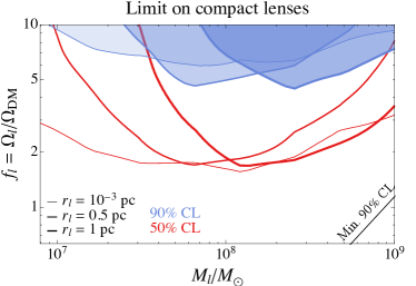
Figure 5: Constraints from the MCs velocity template analysis on the fractional dark matter abundance $f_{l}$ of compact objects with mass $M_{l}$ and density profile given in Eq. 3, for different compact object radii $r_{l}=10^{-3},0.5,\text{ and }1~{}\text{pc}$. The constraint for the smallest radius is equivalent to the one for point-like objects ($r_{l}=2G_{N}M_{l}$) given the angular number density of stars. Above the diagonal line at the bottom right, at least one subhalo eclipses the data sample with 90% probability.

VI Discussion

We presented results and limits from the first analysis leveraging precision astrometry data and time-domain weak gravitational lensing to look for Galactic substructure. A simple modification of our analysis technique can also unambigously confirm tentative local lensing signals. The rate of change of impact parameter receives periodic contributions from Earth’s motion around the Sun with known phase, direction, and magnitude of order $30\,\mathrm{km/s}$. This lensing-induced “anomalous parallax” motion is guaranteed to be present if a tentative signal of correlated linear stellar motions is due to astrometric weak lensing. It is almost an order of magnitude smaller, and its error has less favorable scaling with integration time than the linear motion ($\sigma_{\mu,\varpi}/\sigma_{\mu}\sim t_{\mathrm{int}}/\mathrm{1\,yr}$). However, this signature will always be statistics-limited insofar that it cannot be faked by intrinsic stellar motions. This latter observation opens up the possibility of astrometric lensing searches for dark matter on Gaia’s entire data set (once time-series data becomes available), including more precisely measured nearby stars rather than the distant MCs.

Our constraints are statistics-limited now and for the foreseeable future, as the figure-of-merit $\sqrt{\Sigma}/\sigma_{\mu,\mathrm{eff}}$ is largest for relatively faint stars with $\mathrm{G}>16$ and the vast majority of MC stars have $\mathrm{G}>19$. With integration time $t_{\mathrm{int}}$, currently at 22 months for Gaia DR2, we expect the proper motion error to scale at least as fast as $\sigma_{\mu,\mathrm{eff}}\propto t_{\mathrm{int}}^{-3/2}$. The scaling will likely be faster as more stars are added, binaries and double stars are resolved, and modeling of telescope systematics improves with time. Note that Eq. 8 is valid for $r_{l}\gtrsim 1\,\mathrm{pc}$ in this context and that the closest lens at $\langle\min_{l}D_{l}\rangle\propto(M_{l}/f_{l})^{1/3}$ drives the sensitivity. We project that the sensitivity to the combination $f_{l}M_{l}^{2}/r_{l}^{3}$ will improve as $\sigma_{\mu,\mathrm{eff}}^{3}\propto t_{\mathrm{int}}^{-9/2}$ or better, yielding promising prospects for future data releases from Gaia and other astrometric surveys.

Appendix A Appendix

A.1 Derivation of optimal discriminant

We present the derivation of our likelihood-inspired test-statistic $\mathcal{R}$, a global analog of the local test-statistic $\mathcal{T}$ that appropriately weighs over all possible lens locations, angular sizes and velocity directions. Ideally, we would like to check whether the stellar proper motions $\{\bm{\mathbf{\mu}}_{i}\}$ observed across a certain patch of the sky are compatible with the proper motion distortions induced by a population of foreground lenses. The full likelihood function for a lens population is hardly tractable due to the large number of random variables involved. However, we can simplify it by including only the contribution from a single lens, noting that the local signal-to-noise ratio is driven by the closest one (see Eq. 8). In addition, we regard the measured stellar proper motions as independent Gaussian random variables with zero (subtracted) mean. Within this approximation, the likelihood function for a single lens originating from a population of lenses with mass $M_{l}$, characteristic physical size $r_{l}$ and fractional abundance $f_{l}=\Omega_{l}/\Omega_{\mathrm{DM}}$ reads

$$\mathcal{L}\left(\{\bm{\mathbf{\mu}}_{i}\}\big{|}M_{l},r_{l},f_{l}\right)=p_{1}(\bm{\mathbf{\theta}}_{t},\beta_{t})p_{v}(\bm{\mathbf{v}}_{t})\prod_{i}\frac{\exp\left[-\frac{(\bm{\mathbf{\mu}}_{i}-\Delta\bm{\mathbf{\mu}}_{i})^{2}}{2\sigma_{\mu,i}^{2}}\right]}{2\pi\sigma_{\mu,i}^{2}},$$ (10)

where the lens correction $\Delta\bm{\mathbf{\mu}}_{i}$ is given by Eq. 1, $p_{v}$ is the pdf for the tentative lens velocity $\bm{\mathbf{v}}_{t}$ from Eq. 5, and $p_{1}$ corresponds to a joint pdf for the tentative lens position $\bm{\mathbf{\theta}}_{t}$ and size $\beta_{t}$

$$p_{1}(\bm{\mathbf{\theta}}_{t},\beta_{t})=\frac{r_{l}^{3}\rho(\bm{\mathbf{\theta}}_{t},r_{l}/\beta_{t})}{\beta_{t}^{4}M_{l}\langle N_{l}\rangle},$$ (11)

with $\rho(\bm{\mathbf{r}})$ in Eq. 4, and $\langle N_{l}\rangle$ the expected number of lenses in front of the stellar target. The log-likelihood ratio gives

$$\ln\frac{\mathcal{L}\left(\{\bm{\mathbf{\mu}}_{i}\}\big{|}M_{l},r_{l},f_{l}\right)}{\mathcal{L}\left(\{\bm{\mathbf{\mu}}_{i}\}\big{|}\text{no lens}\right)} =\ln\frac{r_{l}^{3}}{M_{l}\langle N_{l}\rangle}+\ln\frac{\rho(\bm{\mathbf{\theta}}_{t},r_{l}/\beta_{t})}{\beta_{t}^{4}}-\frac{\left(\bm{\mathbf{v}}_{t}-\bm{\mathbf{v}}_{0}\right)^{2}}{2\sigma_{v}^{2}}+C\bm{\mathbf{\mathcal{T}}}\cdot\bm{\mathbf{v}}_{t}-\frac{C^{2}v_{t}^{2}\mathcal{N}^{2}}{2},$$ (12)

where $C=4G_{N}M_{l}/r_{l}^{2}$, and we have introduced $\bm{\mathbf{\mathcal{T}}}\equiv\{\mathcal{T}(\theta_{t},\beta_{t},\bm{\mathbf{\hat{\alpha}}}),\mathcal{T}(\theta_{t},\beta_{t},\bm{\mathbf{\hat{\delta}}})\}$, with $\mathcal{T}$ defined in Eq. 6. The normalization factor is defined in Eq. 7; in the limit of a large number of stars distributed in a circularly symmetric way around $\bm{\mathbf{\theta}}_{t}$, it approaches:

$$\mathcal{N}^{2}(\bm{\mathbf{\theta}}_{t},\beta_{t})\simeq\sum_{i}\frac{\beta_{t}^{4}/\beta_{it}^{4}}{\sigma_{\mu,i}^{2}}\left[\widetilde{M}_{l}^{2}+\frac{(\partial\widetilde{M}_{l})^{2}}{2\beta_{t}^{2}/\beta_{it}^{2}}-\frac{\widetilde{M}_{l}\partial\widetilde{M_{l}}}{\beta_{t}/\beta_{it}}\right].$$ (13)

The optimal test statistic is given by maximizing the likelihood ratio over the unknown parameters $\{\bm{\mathbf{\theta}}_{t},\beta_{t},\hat{\bm{\mathbf{v}}}_{t}\}$. The velocity $\bm{\mathbf{v}}_{t,\mathrm{sup}}$ that maximizes Eq. 12 can be computed explicitly

$$v_{t,\mathrm{sup}} =\frac{|\bm{\mathbf{v}}_{0}+C\sigma_{v}^{2}\bm{\mathbf{\mathcal{T}}}|}{1+C^{2}\sigma_{v}^{2}\mathcal{N}^{2}}$$ (14)

$$\hat{\bm{\mathbf{v}}}_{t,\mathrm{sup}}\cdot\hat{\bm{\mathbf{v}}}_{0} =\frac{C\sigma_{v}^{2}\bm{\mathbf{\mathcal{T}}}\cdot\bm{\mathbf{v}}_{0}+v_{0}^{2}}{v_{0}|\bm{\mathbf{v}}_{0}+C\sigma_{v}^{2}\bm{\mathbf{\mathcal{T}}}|}.$$ (15)

Using the above expression and dropping the constant terms in Eq. 12, we find the expression for the optimal test statistic

$$\mathcal{R} =\sup_{\bm{\mathbf{\theta}}_{t},\beta_{t}}\ln\frac{\mathcal{L}\left(\{\bm{\mathbf{\mu}}_{i}\}\big{|}M_{l},r_{l},f_{l}\right)}{\mathcal{L}\left(\{\bm{\mathbf{\mu}}_{i}\}\big{|}\text{no lens}\right)}\Bigg{|}_{\bm{\mathbf{v}}_{t}=\bm{\mathbf{v}}_{t,\mathrm{sup}}}$$ (16)

given by the expression in Eq. 9.

A.2 Raw data

In this part of the Appendix, we describe our data manipulations in more depth.

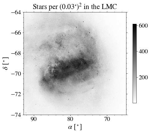
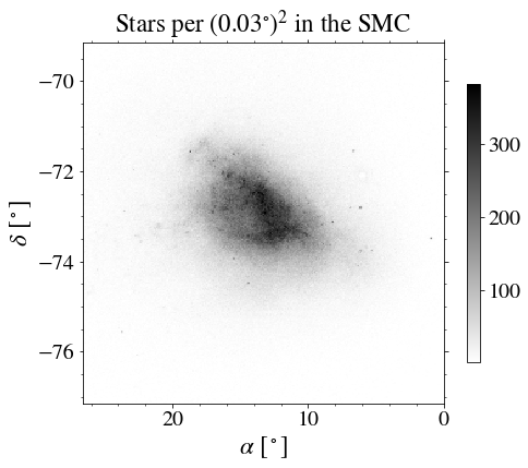
Figure 6: Number density distribution on the sky of the stars selected from the Large Magellanic Cloud (top) and Small Magellanic Cloud (bottom).

A.2.1 Data Cleaning

In Fig. 6, we plot the stellar surface densities of the Magellanic Clouds (MCs), as they appear in the second data release of Gaia Prusti et al. (2016); Brown et al. (2018) for the selected 14,017,189 stars of the Large Magellanic Cloud (LMC) and the 1,890,713 stars of the Small Magellanic Cloud (SMC). Before applying the template analysis to the chosen stellar targets, we address systematics whose potential contributions to the proper motions of the stars could be misconstrued as a lensing signal. One source of contamination comes from overdense stellar clusters, which we remove by comparing a pixelated angular number density map $\Sigma(\bm{\mathbf{\theta}})$ in pixels of size $\beta_{sm}/3$ with an average local number density map, smoothed with a Gaussian distance kernel of size $\beta_{\rm{sm}}=0.1^{\circ}$:

$$\Sigma_{\rm{sm}}(\bm{\mathbf{\theta}})=\frac{\int{\rm d}\bm{\mathbf{\theta^{\prime}}}\exp\left[-\frac{(\bm{\mathbf{\theta}}-\bm{\mathbf{\theta^{\prime}}})^{2}}{2\beta_{\rm{sm}}^{2}}\right]\Sigma(\bm{\mathbf{\theta^{\prime}}})}{\int{\rm d}\bm{\mathbf{\theta^{\prime}}}\exp\left[-\frac{(\bm{\mathbf{\theta}}-\bm{\mathbf{\theta^{\prime}}})^{2}}{2\beta_{\rm{sm}}^{2}}\right]}.$$ (17)

We remove pixels for which $\Sigma(\bm{\mathbf{\theta}})>3\Sigma_{\rm{sm}}(\bm{\mathbf{\theta}})$, reducing the initial LMC and SMC star populations by $0.03\%$ and $0.10\%$, respectively.

To account for the coherent velocity fields present in the data, we define a smoothed average local proper motion field $\bm{\mathbf{\mu}}_{\rm{sm}}(\bm{\mathbf{\theta}})$, again with a Gaussian kernel of angular size $\beta_{\rm{sm}}$

$$\bm{\mathbf{\mu}}_{\rm{\rm{sm}}}(\bm{\mathbf{\theta}})=\frac{\int{\rm d}\bm{\mathbf{\theta^{\prime}}}\exp\left[-\frac{(\bm{\mathbf{\theta}}-\bm{\mathbf{\theta^{\prime}}})^{2}}{2\beta_{\rm{sm}}^{2}}\right]\bm{\mathbf{\mu}}(\bm{\mathbf{\theta^{\prime}}})}{\int{\rm d}\bm{\mathbf{\theta^{\prime}}}\exp\left[-\frac{(\bm{\mathbf{\theta}}-\bm{\mathbf{\theta^{\prime}}})^{2}}{2\beta_{\rm{sm}}^{2}}\right]},$$ (18)

and subtract it from the local proper motion field $\bm{\mathbf{\mu}}(\bm{\mathbf{\theta}}_{p})=\sum_{i\in p}\bm{\mathbf{\mu}}_{i}\sigma_{\mu,i}^{-2}/\sum_{i\in p}\sigma_{\mu,i}^{-2}$, in square pixels of size $0.05^{\circ}$, to obtain $\bm{\mathbf{\mu}}_{\mathrm{sub},i}\equiv\bm{\mathbf{\mu}}_{i}-\bm{\mathbf{\mu}}_{\mathrm{sm}}(\bm{\mathbf{\theta}}_{i})$. We cut out “velocity outliers”—gravitationally unbound, high-velocity stars—that do not satisfy the relation $\mu_{\mathrm{sub},i}>3\sigma_{\mu,i}+\mu_{\mathrm{esc}}$, where we take $\mu_{\rm{esc}}=0.2$ mas/y as the (proper) escape velocity for both of the MCs. Removing velocity outliers causes the local mean proper motion to shift away from zero again. For this reason, we repeat the background motion subtraction and removal of outliers for a total of 3 iterations. The fraction of outliers in the last iteration is small enough to guarantee a final sample whose mean proper motion is consistent with zero. The velocity subtraction by means of a Gaussian distance kernel introduces edge artifacts of size $\sim\beta_{\rm{sm}}$ at each iteration, which we avoid by rejecting stars within $6\times\beta_{\rm{sm}}$ from the edges. Table 1 summarizes the fraction of stars removed from the original Gaia sample during each cleaning procedure. In Fig. 7, we present the proper motion distribution of the LMC data with dense clusters removed, before (top panels) and after (bottom panels) the large-scale motion subtraction and removal of velocity outliers.

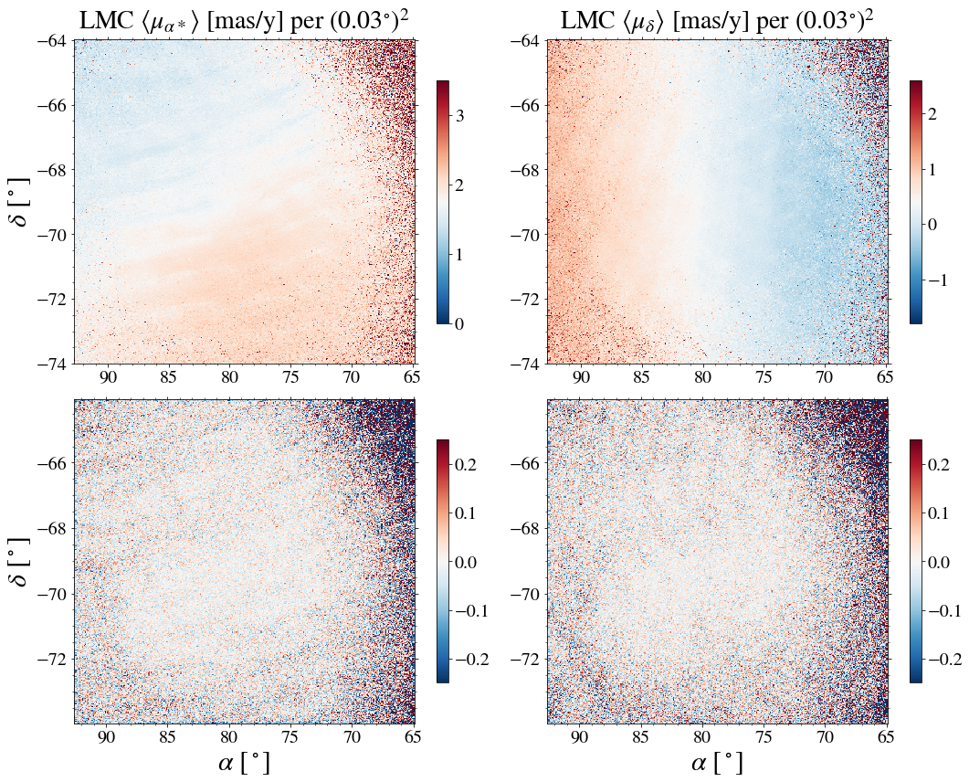
Figure 7: Average stellar proper motion across the LMC, $\langle\mu\rangle\equiv\sum_{i\in p}\mu_{i}\sigma^{-2}_{\mu,i}/\sum_{i\in p}\sigma^{-2}_{\mu,i}$ per pixels of size $0.03^{\circ}$ in the RA (left) and DEC (right) directions. The top panel shows the proper motion field in the original Gaia data sample after the removal of dense clusters, and the bottom panel after additional background motion subtraction and removal of outliers.

Number of stars removed
Cleaning procedure	LMC	SMC
dense clusters	$0.03\%$	$0.10\%$
velocity outliers, iter 1	$5.32\%$	$0.66\%$
velocity outliers, iter 2	$0.05\%$	$<0.01\%$
velocity outliers, iter 3	$<0.01\%$	$<0.01\%$
edges	$6.91\%$	$2.79\%$

Table 1: Percentage decrease in the selected stellar populations due to the cleaning procedures described in the text.

A.2.2 Calculation of the effective error

This part of our data treatment deals with the spread and uncertainties in the stellar proper motions. In general, the astrometric performance of $\it{Gaia}$ can be impacted by noise contributions both stochastic and systematic in nature. Even if we are in no position to precisely identify all the potential noise sources, the best way to acknowledge their presence is by calculating the mean effective variance $\sigma^{2}_{\rm{\mu,eff}}$. Since the precision of the astrometric measurements depends on the apparent brightness of the sources, we bin the stars in G-magnitude and calculate the effective dispersion in each bin. This quantity virtually encapsulates the instrumental errors, intrinsic dispersion, as well as artifacts of crowding, unresolved binaries, and potential residual trends in the stellar motions that were not successfully removed during the velocity subtraction. In each bin of $0.1$ in G-magnitude we contrast the mean observed effective error, $\sigma^{2}_{\rm{\mu,eff}}\equiv\langle\mu_{\alpha*}^{2}+\mu_{\delta}^{2}\rangle$, to the Gaia-reported formal error of each star, $\sigma_{\mu_{i}}^{2}\equiv\sigma_{\mu_{i,\alpha}}^{2}+\sigma_{\mu_{i,\delta}}^{2}$. In the vast majority of cases, the former exceeds the latter; in the computation of the test statistic $\mathcal{T}$, we weigh each star by the larger of the two quantities. We can deduce which stars have the best sensitivity for the lensing signal from the signal-to-noise ratio estimate of Eq. 8. The relevant figure of merit to be maximized is $\sqrt{\Sigma}/\sigma_{\mu}$, where $\Sigma\propto N_{s}$ is the typical angular number density of a population of $N_{s}$ stars in the observed patch of the sky. As displayed in Fig. 8, the best sensitivity is currently coming from the population of stars with $16\lesssim G\lesssim 19$. Though the $\it Gaia$ DR2 catalog showcases significant advancements compared to DR1, its capabilities in terms of astrometric lensing searches are still far from their ultimate end-of-mision values due to the relatively short observational period. This current dataset still contains partial instrumental calibration errors, inadequate background estimation, underestimates of centroid location uncertainties, and mislabeling of the sources’ properties, among other unmodelled errors Arenou et al. (2018); Lindegren et al. (2018). The improvement of such issues in view of the increased time span of the operational phase, along with the scaling of the proper motion error with time as $t_{\rm{int}}^{-3/2}$, are bound to drive up the value of the figure of merit in the near future.

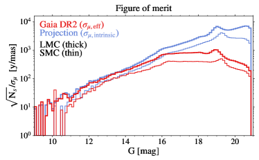
Figure 8: Figure of merit for the template velocity observable $\sqrt{N_{s}}/\sigma_{\mu}$ as a function of G-magnitude in the LMC (thick) and SMC (thin). $N_{s}$ is the number of stars per G-magnitude bin and $\sigma_{\mu}$ defined as in Fig. 3. The best sensitivity for the signal is given by the stars that maximize the figure of merit, i.e. with $16\lesssim G\lesssim 19$ in Gaia DR2 (red) and potentially by the most numerous fainter stars when the measurements will reach the intrinsic proper motion dispersion floor (blue).

A.3 Template method details

To perform the template scanning at a given angular scale $\beta_{t}$, the stars are pixelated with pixel size $0.1\times\beta_{t}$. We first scan coarsely every 9 lattice sites, computing $\mathcal{T}$ as defined in Eq. 6, along the horizontal ($\hat{\bm{\mathbf{v}}}_{t}=\bm{\mathbf{\hat{\alpha}}}$) and vertical ($\hat{\bm{\mathbf{v}}}_{t}=\bm{\mathbf{\hat{\delta}}}$) directions, and $\mathcal{N}$ as defined in Eq. 13, using a masking matrix kernel of size $\beta_{\mathrm{mask}}=\mathrm{max}(4\times\beta_{t},0.01^{\circ})$. The normalization factors obtained from the MCs scanning at 4 different angular scales are displayed in Fig. 9. For a uniformly distributed set of background sources with angular number density $\Sigma$, we expect the distribution and typical value of $\mathcal{N}/\beta_{t}\sim\sqrt{\Sigma}/\sigma_{\mu}$ to be independent of $\beta_{t}$, a behavior borne out in the data for $\beta_{t}\gtrsim 0.004^{\circ}$. The expected scaling breaks down for $\beta_{t}$ values smaller than the typical angular separation between two stars, which in practice sets a lower bound on the useful angular scales to be considered for the template.

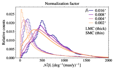
Figure 9: Histograms of the normalization factor defined in Eq. 13 at selected angular scales $\beta_{t}$ for the LMC (thick) and the SMC (thin). The expected scaling $\mathcal{N}/\beta_{t}\sim\sqrt{\Sigma}/\sigma_{\mu}$ is observed in the data for $\beta_{t}\gtrsim 0.004^{\circ}$, and breaks down at scales smaller than the typical angular separation between two stars.

For each parameter space point $\{M_{l},r_{l},f_{l}\}$ we compute the optimal template angular scale $\beta_{t,\rm{opt}}$, defined by requiring 3 expected lenses in front of the stellar targets with $\beta_{l}\geq\beta_{t,\rm{opt}}$. We then select from the fixed list of 58 $\beta_{t}$ values the 3 closest to $\beta_{t,\rm{opt}}$ (or the 2 closest if $\beta_{t,\rm{opt}}\leq 0.0015^{\circ}$ or $\beta_{t,\rm{opt}}\geq 0.03^{\circ}$). This subset is used to perform the template scanning on a fine grid with lattice constant $\beta_{\mathrm{scan}}=0.1\times\beta_{t}$ on squares of size $\beta_{t}$ centered at the location of the simulated lenses (only the 200 closest lenses are retained). The list of $\{\mathcal{T}_{\alpha},\mathcal{T}_{\delta},\mathcal{N}\}$ values obtained is used to compute the test statistic $\mathcal{R}$ to be compared with the value resulting from the coarse+fine scan of both the LMC and SMC data using the same subset of $\beta_{t}$ values. For computational efficiency, we only compute the test statistic in locations where $C\sigma_{v}\mathcal{N}>1$, as we do not expect a large signal elsewhere.

A.4 Lens density profiles

The analysis presented in the main text is repeated using a velocity template that ignores the details of the inner density profile of the lens by truncating the signal at angular distances $>\beta_{l}$. In Eq. 2 we take $\widetilde{M}_{l}(\beta_{il})=\Theta(\beta_{il}-\beta_{l})$ and $\partial_{\beta_{il}}\widetilde{M}(\beta_{il})=0$, obtaining the universal dipole pattern displayed in Fig. 10. The resulting limit on compact lenses from the MCs data analysis is presented in Fig. LABEL:fig:compactlimit_tr in the $(M_{l},f_{l})$ plane for three values of $r_{l}$. The result is comparable to the limit shown in Fig. 5 obtained using the lens profile of Eq. 3. Note that in the presence of a lens with an unknown profile, the analysis using the truncated velocity template would still capture a large fraction of the signal. The sensitivity is expected to improve by an $\mathcal{O}(1)$ factor when choosing the velocity template that exactly matches the distortion produced by the true lens.

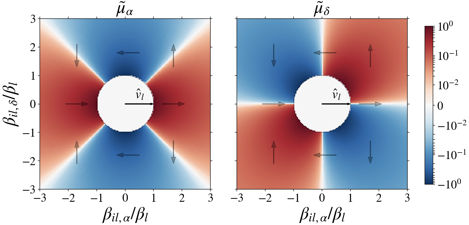
Figure 10: Right-ascension ($\alpha$, left) and declination ($\delta$, right) components of the angular velocity vector profile $\tilde{\bm{\mathbf{\mu}}}_{i}$ of Eq. 2 as a function of angular separation $\bm{\mathbf{\beta}}_{il}$ taking $\widetilde{M}_{l}(\beta_{il})=\Theta(\beta_{il}-\beta_{l})$ and $\partial_{\beta_{il}}\widetilde{M}(\beta_{il})=0$. The lens has angular size $\beta_{l}$ and is moving in the direction $\hat{\bm{\mathbf{v}}}_{l}=\hat{\bm{\mathbf{v}}}_{\alpha}$.

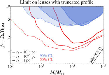
Figure 11: Constraints from the MCs velocity template analysis on the fractional dark matter abundance $f_{l}$ of compact objects with mass $M_{l}$ and density profile truncated at $r_{l}$, for different compact object radii $r_{l}=10^{-3},10^{-2},\text{ and }1~{}\text{pc}$. The constraint for the smallest radius is equivalent to the one for point-like objects ($r_{l}=2G_{N}M_{l}$) given the angular number density of stars. Above the diagonal line at the bottom right, at least one subhalo eclipses the data sample with 90% probability.

References

- Ade et al. (2016a) P. A. Ade, N. Aghanim, M. Arnaud, M. Ashdown, J. Aumont, C. Baccigalupi, A. Banday, R. Barreiro, J. Bartlett, N. Bartolo, et al., Astronomy & Astrophysics 594, A13 (2016a).
- Aghanim et al. (2018) N. Aghanim, Y. Akrami, M. Ashdown, J. Aumont, C. Baccigalupi, M. Ballardini, A. Banday, R. Barreiro, N. Bartolo, S. Basak, et al., arXiv preprint arXiv:1807.06209 (2018).
- Seljak et al. (2006) U. Seljak, A. Slosar, and P. McDonald, Journal of Cosmology and Astroparticle Physics 2006, 014 (2006).
- Blomqvist et al. (2019) M. Blomqvist, H. d. M. d. Bourboux, N. G. Busca, V. d. S. Agathe, J. Rich, C. Balland, J. E. Bautista, K. Dawson, A. Font-Ribera, J. Guy, et al., arXiv preprint arXiv:1904.03430 (2019).
- Agathe et al. (2019) V. d. S. Agathe, C. Balland, H. d. M. d. Bourboux, N. G. Busca, M. Blomqvist, J. Guy, J. Rich, A. Font-Ribera, M. M. Pieri, J. E. Bautista, et al., arXiv preprint arXiv:1904.03400 (2019).
- Percival and White (2009) W. J. Percival and M. White, Monthly Notices of the Royal Astronomical Society 393, 297 (2009).
- Howlett et al. (2015) C. Howlett, A. J. Ross, L. Samushia, W. J. Percival, and M. Manera, Monthly Notices of the Royal Astronomical Society 449, 848 (2015).
- Zarrouk et al. (2018) P. Zarrouk, E. Burtin, H. Gil-Marín, A. J. Ross, R. Tojeiro, I. Pâris, K. S. Dawson, A. D. Myers, W. J. Percival, C.-H. Chuang, et al., Monthly Notices of the Royal Astronomical Society 477, 1639 (2018).
- Springel et al. (2008) V. Springel, J. Wang, M. Vogelsberger, A. Ludlow, A. Jenkins, A. Helmi, J. F. Navarro, C. S. Frenk, and S. D. White, Monthly Notices of the Royal Astronomical Society 391, 1685 (2008).
- Diemand et al. (2008) J. Diemand, M. Kuhlen, P. Madau, M. Zemp, B. Moore, D. Potter, and J. Stadel, Nature 454, 735 (2008).
- Boylan-Kolchin et al. (2009) M. Boylan-Kolchin, V. Springel, S. D. White, A. Jenkins, and G. Lemson, Monthly Notices of the Royal Astronomical Society 398, 1150 (2009).
- Stadel et al. (2009) J. Stadel, D. Potter, B. Moore, J. Diemand, P. Madau, M. Zemp, M. Kuhlen, and V. Quilis, Monthly Notices of the Royal Astronomical Society: Letters 398, L21 (2009).
- Garrison-Kimmel et al. (2014) S. Garrison-Kimmel, M. Boylan-Kolchin, J. S. Bullock, and K. Lee, Monthly Notices of the Royal Astronomical Society 438, 2578 (2014).
- Vogelsberger et al. (2014) M. Vogelsberger, S. Genel, V. Springel, P. Torrey, D. Sijacki, D. Xu, G. Snyder, D. Nelson, and L. Hernquist, Monthly Notices of the Royal Astronomical Society 444, 1518 (2014).
- Hellwing et al. (2016) W. A. Hellwing, C. S. Frenk, M. Cautun, S. Bose, J. Helly, A. Jenkins, T. Sawala, and M. Cytowski, Monthly Notices of the Royal Astronomical Society 457, 3492 (2016).
- Rubin and Ford Jr (1970) V. C. Rubin and W. K. Ford Jr, The Astrophysical Journal 159, 379 (1970).
- Freeman (1970) K. C. Freeman, The Astrophysical Journal 160, 811 (1970).
- Rogstad and Shostak (1972) D. Rogstad and G. Shostak, The Astrophysical Journal 176, 315 (1972).
- Whitehurst and Roberts (1972) R. N. Whitehurst and M. S. Roberts, The Astrophysical Journal 175, 347 (1972).
- Roberts and Rots (1973) M. Roberts and A. Rots, Astronomy and Astrophysics 26, 483 (1973).
- Zwicky (1933) F. Zwicky, Helvetica Physica Acta 6, 110 (1933).
- Smith (1936) S. Smith, The Astrophysical Journal 83, 23 (1936).
- Zwicky (1937) F. Zwicky, The Astrophysical Journal 86, 217 (1937).
- Girardi et al. (1998) M. Girardi, G. Giuricin, F. Mardirossian, M. Mezzetti, and W. Boschin, The Astrophysical Journal 505, 74 (1998).
- Rines and Diaferio (2006) K. Rines and A. Diaferio, The Astronomical Journal 132, 1275 (2006).
- Becker et al. (2007) M. R. Becker, T. McKay, B. Koester, R. Wechsler, E. Rozo, A. Evrard, D. Johnston, E. Sheldon, J. Annis, E. Lau, et al., The Astrophysical Journal 669, 905 (2007).
- Kaiser and Squires (1993) N. Kaiser and G. Squires, The Astrophysical Journal 404, 441 (1993).
- Schneider (1996) P. Schneider, Monthly Notices of the Royal Astronomical Society 283, 837 (1996).
- Wittman et al. (2000) D. M. Wittman, J. A. Tyson, D. Kirkman, I. Dell’Antonio, and G. Bernstein, Nature 405, 143 (2000).
- Hoekstra et al. (2004) H. Hoekstra, H. K. Yee, and M. D. Gladders, The Astrophysical Journal 606, 67 (2004).
- Okabe et al. (2014) N. Okabe, T. Futamase, M. Kajisawa, and R. Kuroshima, The Astrophysical Journal 784, 90 (2014).
- Keeton (2001) C. R. Keeton, The Astrophysical Journal 561, 46 (2001).
- Treu (2010) T. Treu, Annual Review of Astronomy and Astrophysics 48, 87 (2010).
- Jullo et al. (2010) E. Jullo, P. Natarajan, J.-P. Kneib, A. D’Aloisio, M. Limousin, J. Richard, and C. Schimd, Science 329, 924 (2010).
- Klypin et al. (1999) A. Klypin, A. V. Kravtsov, O. Valenzuela, and F. Prada, The Astrophysical Journal 522, 82 (1999).
- Willman et al. (2004) B. Willman, F. Governato, J. J. Dalcanton, D. Reed, and T. Quinn, Monthly Notices of the Royal Astronomical Society 353, 639 (2004).
- Tollerud et al. (2008) E. J. Tollerud, J. S. Bullock, L. E. Strigari, and B. Willman, The Astrophysical Journal 688, 277 (2008).
- Rees and Ostriker (1977) M. J. Rees and J. Ostriker, Monthly Notices of the Royal Astronomical Society 179, 541 (1977).
- Kravtsov (2010) A. Kravtsov, Advances in Astronomy 2010 (2010).
- Bromm (2013) V. Bromm, Reports on Progress in Physics 76, 112901 (2013).
- Mao and Schneider (1998) S. Mao and P. Schneider, Monthly Notices of the Royal Astronomical Society 295, 587 (1998).
- Metcalf and Madau (2001) R. B. Metcalf and P. Madau, The Astrophysical Journal 563, 9 (2001).
- Chiba (2002) M. Chiba, The Astrophysical Journal 565, 17 (2002).
- Dalal and Kochanek (2002) N. Dalal and C. Kochanek, The Astrophysical Journal 572, 25 (2002).
- Metcalf and Zhao (2002) R. B. Metcalf and H. Zhao, The Astrophysical Journal Letters 567, L5 (2002).
- Koopmans et al. (2002) L. Koopmans, M. Garrett, R. Blandford, C. Lawrence, A. Patnaik, and R. Porcas, Monthly Notices of the Royal Astronomical Society 334, 39 (2002).
- Kochanek and Dalal (2004) C. Kochanek and N. Dalal, The Astrophysical Journal 610, 69 (2004).
- Inoue and Chiba (2005a) K. T. Inoue and M. Chiba, The Astrophysical Journal 633, 23 (2005a).
- Inoue and Chiba (2005b) K. T. Inoue and M. Chiba, The Astrophysical Journal 634, 77 (2005b).
- Koopmans (2005) L. Koopmans, Monthly Notices of the Royal Astronomical Society 363, 1136 (2005).
- Chen et al. (2007) J. Chen, E. Rozo, N. Dalal, and J. E. Taylor, The Astrophysical Journal 659, 52 (2007).
- Williams et al. (2008) L. L. Williams, P. Foley, D. Farnsworth, and J. Belter, The Astrophysical Journal 685, 725 (2008).
- More et al. (2009) A. More, J. McKean, S. More, R. Porcas, L. Koopmans, and M. Garrett, Monthly Notices of the Royal Astronomical Society 394, 174 (2009).
- Keeton and Moustakas (2009) C. R. Keeton and L. A. Moustakas, The Astrophysical Journal 699, 1720 (2009).
- Vegetti and Koopmans (2009a) S. Vegetti and L. V. Koopmans, Monthly Notices of the Royal Astronomical Society 392, 945 (2009a).
- Vegetti and Koopmans (2009b) S. Vegetti and L. Koopmans, Monthly Notices of the Royal Astronomical Society 400, 1583 (2009b).
- Congdon et al. (2010) A. B. Congdon, C. R. Keeton, and C. E. Nordgren, The Astrophysical Journal 709, 552 (2010).
- Hezaveh et al. (2013) Y. Hezaveh, N. Dalal, G. Holder, M. Kuhlen, D. Marrone, N. Murray, and J. Vieira, The Astrophysical Journal 767, 9 (2013).
- Vegetti and Vogelsberger (2014) S. Vegetti and M. Vogelsberger, Monthly Notices of the Royal Astronomical Society 442, 3598 (2014).
- Hezaveh et al. (2016a) Y. Hezaveh, N. Dalal, G. Holder, T. Kisner, M. Kuhlen, and L. P. Levasseur, Journal of Cosmology and Astroparticle Physics 2016, 048 (2016a).
- Hezaveh et al. (2016b) Y. D. Hezaveh, N. Dalal, D. P. Marrone, Y.-Y. Mao, W. Morningstar, D. Wen, R. D. Blandford, J. E. Carlstrom, C. D. Fassnacht, G. P. Holder, et al., The Astrophysical Journal 823, 37 (2016b).
- Feldmann and Spolyar (2014) R. Feldmann and D. Spolyar, Monthly Notices of the Royal Astronomical Society 446, 1000 (2014).
- Buschmann et al. (2017) M. Buschmann, J. Kopp, B. R. Safdi, and C.-L. Wu, arXiv preprint arXiv:1711.03554 (2017).
- Dai et al. (2018) L. Dai, S.-S. Li, B. Zackay, S. Mao, and Y. Lu, Physical Review D 98, 104029 (2018).
- Dai and Miralda-Escudé (2019) L. Dai and J. Miralda-Escudé, arXiv preprint arXiv:1908.01773 (2019).
- Ibata et al. (2002) R. Ibata, G. Lewis, M. Irwin, and T. Quinn, Monthly Notices of the Royal Astronomical Society 332, 915 (2002).
- Johnston et al. (2002) K. V. Johnston, D. N. Spergel, and C. Haydn, The Astrophysical Journal 570, 656 (2002).
- Siegal-Gaskins and Valluri (2008) J. M. Siegal-Gaskins and M. Valluri, The Astrophysical Journal 681, 40 (2008).
- Bovy (2016) J. Bovy, Physical review letters 116, 121301 (2016).
- Carlberg (2016) R. G. Carlberg, The Astrophysical Journal 820, 45 (2016).
- Erkal et al. (2016) D. Erkal, V. Belokurov, J. Bovy, and J. L. Sanders, Monthly Notices of the Royal Astronomical Society 463, 102 (2016).
- Bonaca and Hogg (2018) A. Bonaca and D. W. Hogg, The Astrophysical Journal 867, 101 (2018).
- Bonaca et al. (2018) A. Bonaca, D. W. Hogg, A. M. Price-Whelan, and C. Conroy, arXiv preprint arXiv:1811.03631 (2018).
- Banik et al. (2019) N. Banik, J. Bovy, G. Bertone, D. Erkal, and T. J. L. de Boer, arXiv preprint arXiv:1911.02662 (2019).
- Paczynski (1986) B. Paczynski, The Astrophysical Journal 304, 1 (1986).
- Alcock et al. (2000) C. Alcock, R. Allsman, D. R. Alves, T. Axelrod, A. C. Becker, D. Bennett, K. H. Cook, N. Dalal, A. J. Drake, K. Freeman, et al., The Astrophysical Journal 542, 281 (2000).
- Tisserand et al. (2007) P. Tisserand, L. Le Guillou, C. Afonso, J. Albert, J. Andersen, R. Ansari, É. Aubourg, P. Bareyre, J. Beaulieu, X. Charlot, et al., Astronomy & Astrophysics 469, 387 (2007).
- Griest et al. (2014) K. Griest, A. M. Cieplak, and M. J. Lehner, The Astrophysical Journal 786, 158 (2014).
- Niikura et al. (2017) H. Niikura, M. Takada, N. Yasuda, R. H. Lupton, T. Sumi, S. More, T. Kurita, S. Sugiyama, A. More, M. Oguri, et al., arXiv preprint arXiv:1701.02151 (2017).
- Zumalacarregui and Seljak (2018) M. Zumalacarregui and U. Seljak, Physical review letters 121, 141101 (2018).
- Siegel et al. (2007) E. R. Siegel, M. Hertzberg, and J. Fry, Monthly Notices of the Royal Astronomical Society 382, 879 (2007).
- Seto and Cooray (2007) N. Seto and A. Cooray, The Astrophysical Journal Letters 659, L33 (2007).
- Baghram et al. (2011) S. Baghram, N. Afshordi, and K. M. Zurek, Physical Review D 84, 043511 (2011).
- Kashiyama and Seto (2012) K. Kashiyama and N. Seto, Monthly Notices of the Royal Astronomical Society 426, 1369 (2012).
- Clark et al. (2015) H. A. Clark, G. F. Lewis, and P. Scott, Monthly Notices of the Royal Astronomical Society 456, 1394 (2015).
- Schutz and Liu (2017) K. Schutz and A. Liu, Physical Review D 95, 023002 (2017).
- Dror et al. (2019) J. A. Dror, H. Ramani, T. Trickle, and K. M. Zurek, arXiv preprint arXiv:1901.04490 (2019).
- Van Tilburg et al. (2018) K. Van Tilburg, A.-M. Taki, and N. Weiner, arXiv preprint arXiv:1804.01991 (2018).
- Ade et al. (2016b) P. Ade, N. Aghanim, M. Arnaud, F. Arroja, M. Ashdown, J. Aumont, C. Baccigalupi, M. Ballardini, A. Banday, R. Barreiro, et al., Astronomy & Astrophysics 594, A20 (2016b).
- Akrami et al. (2018) Y. Akrami, F. Arroja, M. Ashdown, J. Aumont, C. Baccigalupi, M. Ballardini, A. Banday, R. Barreiro, N. Bartolo, S. Basak, et al., arXiv preprint arXiv:1807.06211 (2018).
- Bird et al. (2011) S. Bird, H. V. Peiris, M. Viel, and L. Verde, Monthly Notices of the Royal Astronomical Society 413, 1717 (2011).
- Zurek et al. (2007) K. M. Zurek, C. J. Hogan, and T. R. Quinn, Physical Review D 75, 043511 (2007).
- Buschmann et al. (2019) M. Buschmann, J. W. Foster, and B. R. Safdi, arXiv preprint arXiv:1906.00967 (2019).
- Colin et al. (2000) P. Colin, V. Avila-Reese, and O. Valenzuela, The Astrophysical Journal 542, 622 (2000).
- Bode et al. (2001) P. Bode, J. P. Ostriker, and N. Turok, The Astrophysical Journal 556, 93 (2001).
- Viel et al. (2005) M. Viel, J. Lesgourgues, M. G. Haehnelt, S. Matarrese, and A. Riotto, Physical Review D 71, 063534 (2005).
- Hu et al. (2000) W. Hu, R. Barkana, and A. Gruzinov, Physical Review Letters 85, 1158 (2000).
- Li et al. (2014) B. Li, T. Rindler-Daller, and P. R. Shapiro, Physical Review D 89, 083536 (2014).
- Hui et al. (2017) L. Hui, J. P. Ostriker, S. Tremaine, and E. Witten, Physical Review D 95, 043541 (2017).
- Agrawal and Randall (2017) P. Agrawal and L. Randall, JCAP 1712, 019 (2017), arXiv:1706.04195 [hep-ph] .
- Chang et al. (2019) J. H. Chang, D. Egana-Ugrinovic, R. Essig, and C. Kouvaris, JCAP 1903, 036 (2019), arXiv:1812.07000 [hep-ph] .
- Essig et al. (2019) R. Essig, S. D. McDermott, H.-B. Yu, and Y.-M. Zhong, Physical review letters 123, 121102 (2019).
- Arvanitaki et al. (2019) A. Arvanitaki, S. Dimopoulos, M. Galanis, L. Lehner, J. O. Thompson, and K. Van Tilburg, arXiv preprint arXiv:1909.11665 (2019).
- McMillan (2011) P. J. McMillan, Monthly Notices of the Royal Astronomical Society 414, 2446 (2011).
- Prusti et al. (2016) T. Prusti, J. De Bruijne, A. G. Brown, A. Vallenari, C. Babusiaux, C. Bailer-Jones, U. Bastian, M. Biermann, D. W. Evans, L. Eyer, et al., Astronomy & Astrophysics 595, A1 (2016).
- Brown et al. (2018) A. Brown, A. Vallenari, T. Prusti, J. De Bruijne, C. Babusiaux, C. Bailer-Jones, M. Biermann, D. W. Evans, L. Eyer, F. Jansen, et al., Astronomy & astrophysics 616, A1 (2018).
- Lindegren (2018) L. Lindegren, Gaia Technical Note: GAIA-C3-TN-LU-LL-124-01 (2018).
- Arenou et al. (2018) F. Arenou, X. Luri, C. Babusiaux, C. Fabricius, A. Helmi, T. Muraveva, A. Robin, F. Spoto, A. Vallenari, T. Antoja, et al., Astronomy & Astrophysics 616, A17 (2018).
- Lindegren et al. (2018) L. Lindegren, J. Hernández, A. Bombrun, S. Klioner, U. Bastian, M. Ramos-Lerate, A. De Torres, H. Steidelmüller, C. Stephenson, D. Hobbs, et al., Astronomy & Astrophysics 616, A2 (2018).
- Gyuk et al. (2000) G. Gyuk, N. Dalal, and K. Griest, The Astrophysical Journal 535, 90 (2000).
- Evans and Howarth (2008) C. J. Evans and I. D. Howarth, Monthly Notices of the Royal Astronomical Society 386, 826 (2008).