Self-Directed Online Machine Learning for Topology Optimization
Abstract
Topology optimization by optimally distributing materials in a given domain requires non-gradient optimizers to solve highly complicated problems. However, with hundreds of design variables or more involved, solving such problems would require millions of Finite Element Method (FEM) calculations whose computational cost is huge and impractical. Here we report Self-directed Online Learning Optimization (SOLO) which integrates Deep Neural Network (DNN) with FEM calculations. A DNN learns and substitutes the objective as a function of design variables. A small number of training data is generated dynamically based on the DNN’s prediction of the optimum. The DNN adapts to the new training data and gives better prediction in the region of interest until convergence. The optimum predicted by the DNN is proved to converge to the true global optimum through iterations. Our algorithm was tested by four types of problems including compliance minimization, fluid-structure optimization, heat transfer enhancement and truss optimization. It reduced the computational time by orders of magnitude compared with directly using heuristic methods, and outperformed all state-of-the-art algorithms tested in our experiments. This approach enables solving large multi-dimensional optimization problems.
This paper is published on Nature Communications (https://rdcu.be/cFHgJ)
Main
Distributing materials in a domain to optimize performance is a significant topic in many fields, such as solid mechanics, heat transfer, acoustics, fluid mechanics, materials design and various multiphysics disciplines1. Many numerical approaches2 have been developed since 1988, where the problems are formulated by density, level set, phase field, topological derivative or other methods3. Typically, these approaches use gradient-based optimizers, such as the Method of Moving Asymptotes (MMA), and thus have various restrictions on the properties of governing equations and optimization constraints to allow for fast computation of gradients. Because of the intrinsic limitation of gradient-based algorithms, the majority of existing approaches have only been applied to simple problems, since they would fail as soon as the problem becomes complicated such as involving varying signs on gradients or non-linear constraints4. To address these difficulties, non-gradient methods have been developed which play a significant role in overcoming the tendency to be trapped in a local minimum5.
Non-gradient optimizers, also known as gradient-free or derivative-free methods, do not use the gradient or derivative of the objective function and has been attempted by several researchers, most of which are stochastic and heuristic methods. For instance, Hajela et al. applied Genetic Algorithm (GA) to a truss structure optimization problem to reduce weight6. Shim and Manoochehri minimized the material use subject to maximum stress constraints by a Simulated Annealing (SA) approach7. Besides these two popular methods, other algorithms have been investigated as well, such as ant colonies8, 9, particle swarms10, harmony search11, and bacterial foraging12. Non-gradient methods have four advantages over gradient-based methods5: better optima, applicable to discrete designs, free of gradients and efficient to parallelize. However, the major disadvantage of the methods is their high computational cost from calling the objective functions, which becomes prohibitively expensive for large systems3. As a trade-off, sometimes searching space can be reduced in order for less computation. For instance, pattern search has been applied 13, 14 which is a non-heuristic method with a smaller searching space but is more likely to be trapped in local minima.
Machine learning has been used in sequential model-based optimization (SMBO) to target at expensive objective function evaluation 15, 16. For instance, Bayesian optimization (BO) 17 uses a Gaussian prior to approximate the conditional probability distribution of an objective where is the objective and is the design variable (vector); then the unknown regions can be estimated by the probability model. In Covariance Matrix Adaptation Evolution Strategy (CMA-ES)18, a multivariable Gaussian distribution is used to sample new queries. However, as demonstrated later in the paper, these methods are not designed for large-scale and high-dimensional problems, and thus do not perform well in topology optimization for slow convergence 19 or requirement of shrinking design space 20. Despite some improvement to scale up these algorithms 21, 22, none of them has shown superior performance in topology optimization to the best of our knowledge.
There are some reports on leveraging machine learning to reduce the computational cost of topology optimization23, 24, 25, 26, 27, 28, 29, 30, 31. Most of them are generative models which predict solutions of the same problem under different conditions, after being trained by optimized solutions from gradient-based methods. For example, Yu et al.30 used 100,000 optimal solutions to a simple compliance problem with various boundary forces and the optimal mass fractions to train a neural network consisting of Convolutional Neural Network (CNN) and conditional Generative Adversarial Network (cGAN), which can predict near-optimal designs for any given boundary forces. However, generative models are not topology optimization algorithms: they rely on existing optimal designs as the training data. The predictions are restricted by the coverage of the training datasets. To consider different domain geometries or constraints, new datasets and networks would be required. Besides, the designs predicted by the networks are close to, but still different from the optimal designs. An offline learning method 31 replaces some FEM calculations during the optimization process with DNN’s prediction, yet gives limited improvement especially considering that it requires the solutions to similar problems for training.
Here we propose an algorithm called Self-directed Online Learning Optimization (SOLO) to accelerate non-gradient topology optimization. A DNN is used to map designs to objectives as a surrogate model to approximate and replace the original function which is expensive to calculate. A heuristic optimization algorithm finds the possible optimal design according to DNN’s prediction. Based on the optimum, new query points are dynamically generated and evaluated by the Finite Element Method (FEM) to serve as additional training data. The loop of such self-directed online learning is repeated until convergence. This iterative learning scheme, which can be categorized as an SMBO algorithm, takes advantage of the searching abilities of heuristic methods and the high computational speed of DNN. Theoretical convergence rate is derived under some assumptions. In contrast to gradient-based methods, this algorithm does not rely on gradient information of objective functions of the topology optimization problems. This property allows it to be applied to binary and discrete design variables in addition to continuous ones. To show its performance, we test the algorithm by two compliance minimization problems (designing solid so that the structure achieves maximum stiffness for a given loading), two fluid-structure optimization problems (designing fluid tunnel to minimize the fluid pressure loss for a given inlet speed), a heat transfer enhancement problem (designing a copper structure to reduce the charging time of a heat storage system), and three truss optimization problems (choosing the cross-sectional areas of bars in a truss). Our algorithm reduces the computational cost by at least two orders of magnitude compared with directly applying heuristic methods including Generalized Simulated Annealing (GSA), Binary Bat Algorithm (BBA) and Bat Algorithm (BA). It also outperforms an offline version (where all training data are randomly generated), BO, CMA-ES, and a recent algorithm based on reinforcement learning 32.
Results
Formulation and overview. Consider the following topology optimization problem: in a design domain , find the material distribution that could take either 0 (void) or 1 (solid) at point to minimize the objective function , subject to a volume constraint and possibly other constraints 4. Mathematically, this problem can be written as looking for a function defined on the domain ,
| (1) |
where denotes the given volume. To solve such a problem numerically, the domain is discretized into finite elements to describe the density distribution by nodal or elemental values,
| (2) |
where denotes the weight of integration. The domain of is usually binary (), but more generally may take other values such as discrete () or continuous ().
Our algorithm can be applied to Eq.(2) with binary, discrete or continuous design variables. In this section, we discuss the case of continuous design variables since it is most general.
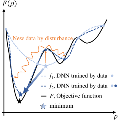
In many applications, the objective function is quite complicated and time-consuming to calculate, since it requires solving partial differential equations by, for instance, FEM. To reduce the number of FEM calculations and accelerate non-gradient optimization, we build a DNN to evaluate the objective function. In a naive way, the entire domain of the objective function should be explored to generate the training data. This would incur a huge number of FEM calculations. However, we only care about the function values close to the global optimum and do not require precise predictions in irrelevant regions. In other words, most information about the objective function in the domain is unnecessary except the details around the optimum. So we do not need to generate data to train in those irrelevant regions.
An intuitive explanation is shown in Fig. 1a. In a 1D minimization example, we can generate a small dataset to train the DNN and refine the mesh around the minimum obtained from the current prediction to achieve higher resolution at the place of interest in the next iteration. After several batches, the minimum of the predicted function would converge to that of the objective function.
 \SetHorizontalCoffin\labelcoffin
a\SetVerticalPole\imagecoffinleft3pt+\CoffinWidth\labelcoffin/2\SetVerticalPole\imagecoffinright\Width-3pt-\CoffinWidth\labelcoffin/2\SetHorizontalPole\imagecoffinup\Height-3pt-\CoffinHeight\labelcoffin/2\SetHorizontalPole\imagecoffindown3pt+\CoffinHeight\labelcoffin/2\JoinCoffins\imagecoffin[left,up]\labelcoffin[vc,hc]\TypesetCoffin\imagecoffin
 \SetHorizontalCoffin\labelcoffin
b\SetVerticalPole\imagecoffinleft3pt+\CoffinWidth\labelcoffin/2\SetVerticalPole\imagecoffinright\Width-3pt-\CoffinWidth\labelcoffin/2\SetHorizontalPole\imagecoffinup\Height-3pt-\CoffinHeight\labelcoffin/2\SetHorizontalPole\imagecoffindown3pt+\CoffinHeight\labelcoffin/2\JoinCoffins\imagecoffin[left,up]\labelcoffin[vc,hc]\TypesetCoffin\imagecoffin
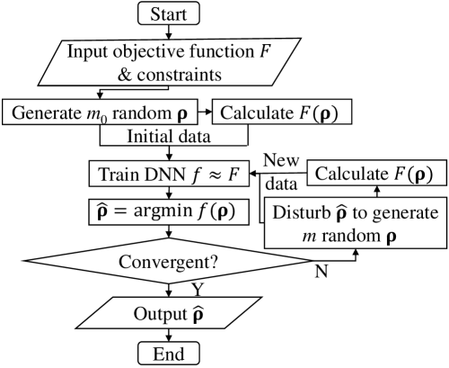
Fig. 1b shows the flow diagram of the proposed algorithm. A small batch of random vectors (or arrays) satisfying the constraints in Eq.(2) is generated. The corresponding objective values are calculated by FEM. Then, and are inputted into the DNN as the training data so that the DNN has a certain level of ability to predict the function values based on the design variables. Namely, the output of the DNN approximates the objective function . Next, the global minimum of the objective function is calculated by a heuristic algorithm. After obtaining the optimized array , more training data are generated accordingly. Inspired by the concept of GA 33, the disturbance we add to the array is more than a small perturbation, and is categorized as mutation, crossover and convolution. Mutation means replacing one or several design variables with random numbers; crossover means exchanging several values in the array; convolution means applying a convolution filter to the variables (see Methods for details). Then constraints are checked and enforced. The self-directed learning and optimization process stops when the value of the objective function does not change anymore or the computation budget is exhausted.
This algorithm can converge provably under some mild assumptions. Given the total number of training data , for any trained DNN with small training error, we have
| (3) |
where is a constant related to some inherent properties of and DNN, is the global minimum of , and omits terms. This result states that when our trained DNN can fit the training data well, then our algorithm can converge to the global optimal value. We provide convergence guarantee with concrete convergence rate for our proposed algorithm, and to the best of our knowledge, this is the first non-asymptotic convergence result for heuristic optimization methods using DNN as a surrogate model. The detailed theory and its derivation are elaborated in Supplementary Section 2.
In the following, we will apply the algorithm to eight classic examples of four types (covering binary, discrete and continuous variables): two compliance minimization problems, two fluid-structure optimization problems, a heat transfer enhancement problem and three truss optimization problems.
Compliance minimization. We first test the algorithm on two simple continuous compliance minimization problems. We show that our algorithm can converge to global optimum and is faster than other non-gradient methods.
 \SetHorizontalCoffin\labelcoffin
a\SetVerticalPole\imagecoffinleft3pt+\CoffinWidth\labelcoffin/2\SetVerticalPole\imagecoffinright\Width-3pt-\CoffinWidth\labelcoffin/2\SetHorizontalPole\imagecoffinup\Height-3pt-\CoffinHeight\labelcoffin/2\SetHorizontalPole\imagecoffindown3pt+\CoffinHeight\labelcoffin/2\JoinCoffins\imagecoffin[left,up]\labelcoffin[vc,hc]\TypesetCoffin\imagecoffin
 \SetHorizontalCoffin\labelcoffin
b\SetVerticalPole\imagecoffinleft3pt+\CoffinWidth\labelcoffin/2\SetVerticalPole\imagecoffinright\Width-3pt-\CoffinWidth\labelcoffin/2\SetHorizontalPole\imagecoffinup\Height-3pt-\CoffinHeight\labelcoffin/2\SetHorizontalPole\imagecoffindown3pt+\CoffinHeight\labelcoffin/2\JoinCoffins\imagecoffin[left,up]\labelcoffin[vc,hc]\TypesetCoffin\imagecoffin
 \SetHorizontalCoffin\labelcoffin
c\SetVerticalPole\imagecoffinleft3pt+\CoffinWidth\labelcoffin/2\SetVerticalPole\imagecoffinright\Width-3pt-\CoffinWidth\labelcoffin/2\SetHorizontalPole\imagecoffinup\Height-3pt-\CoffinHeight\labelcoffin/2\SetHorizontalPole\imagecoffindown3pt+\CoffinHeight\labelcoffin/2\JoinCoffins\imagecoffin[left,up]\labelcoffin[vc,hc]\TypesetCoffin\imagecoffin
d Gradient-based
e SOLO@501
f SOLO@5,782
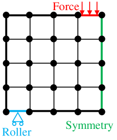
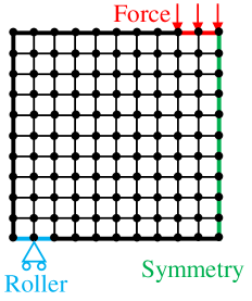
As shown in Fig. 2a, a square domain is divided evenly by a mesh. A force downward is applied at the top right edge; the bottom left edge is set as a roller (no vertical displacement); the right boundary is set to be symmetric. There are 25 nodal design variables to control the material distribution, i.e. density . Our goal is to find the density , subject to a volume constraint of 0.5, such that the elastic energy of the structure is minimized, equivalent to minimizing compliance or the vertical displacement where the external force is applied. Formally,
| (4) |
where . The constraint is
| (5) |
where denotes the vector of linear Gaussian quadrature. In Eq.(4) we use the dimensionless elastic energy , defined as the ratio of elastic energy of the structure with given material distribution to that of the reference uniform distribution (the material density is 0.5 everywhere in the domain). The elastic energy is calculated by FEM from the Young’s modulus in the domain, which is related to density by the popular Simplified Isotropic Material with Penalization (SIMP) method,34
| (6) |
where and denote the Young’s moduli as a variable and a constant respectively, is a small number to avoid numerical singularity and is the material density at a given location interpolated linearly by the nodal values of the element.
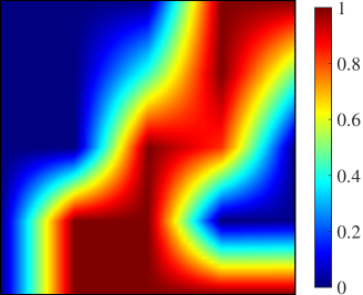
For benchmark, we use a traditional gradient-based algorithm, the Method of Moving Asymptotes (MMA), to find the optimized solution (Fig. 2d).
For our proposed method, we use 100 random arrays to initialize the DNN. Then Generalized Simulated Annealing (GSA) is used to obtain the minimum based on the DNN’s prediction. Afterwards, 100 additional samples will be generated by adding disturbance to including mutation and crossover. Such a loop continues until convergence.
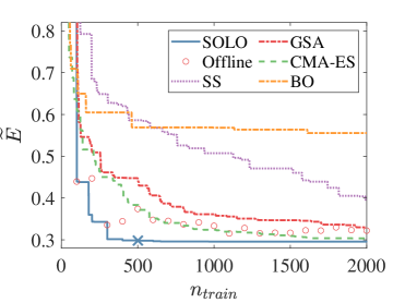
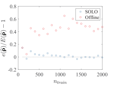
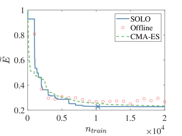
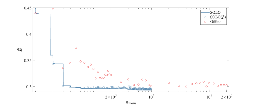
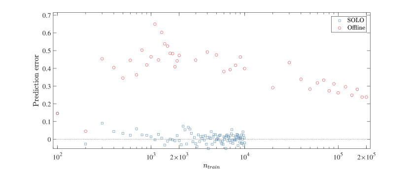
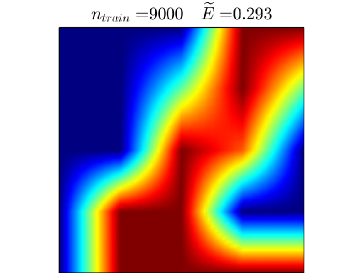
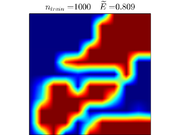
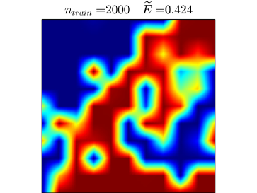
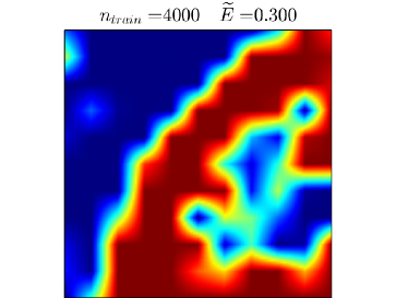
We compare our proposed method, Self-directed Online Learning Optimization (SOLO), with five other algorithms. In Fig. 2b, SOLO converges at . “Offline” denotes a naive implementation to couple DNN with GSA, which trains a DNN offline by random samples and then uses GSA to search for the optimum, without updating the DNN. As expected, the elastic energy decreases with the number of accumulated training samples . This is because more training data will make the DNN estimate the elastic energy more accurately. Yet it converges much slower than SOLO and does not work well even with . More results are shown in Supplementary Fig. 1. SS denotes Stochastic Search, which uses current minimum (the minimum of existing samples) to generate new searching samples; the setup is the same as SOLO except that the base design is obtained from the current minimum instead of a DNN. Comparing SS with SOLO, we can conclude that the DNN in SOLO gives a better searching direction than using existing optima. CMA-ES denotes Covariance Matrix Adaptation Evolution Strategy with a multi-variable Gaussian prior. BO denotes Bayesian Optimization with Gaussian distribution as the prior and expected improvement (EI) as the acquisition function. Our method outperforms all these methods in terms of convergence speed. CMA-ES ranks the second with an objective value 3% higher than SOLO at .
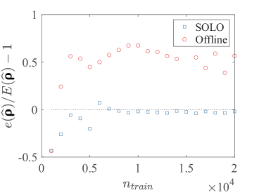
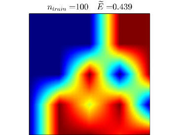
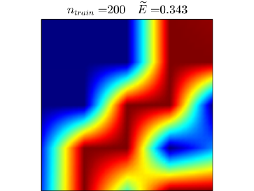
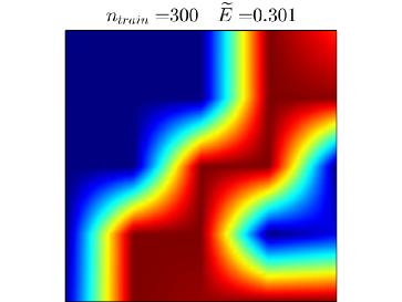
To assess inference accuracy in online and offline learning, we compare the DNN-predicted energy with that calculated by FEM on the same material distribution. The relative error is defined by where and denote energy calculated by DNN and FEM respectively. The energy prediction error is shown in Fig. 2c. When is small, both networks overestimate the energy since their training datasets, composed of randomly distributed density values, correspond to higher energy. As increases, the error of SOLO fluctuates around zero since solutions with low energy are fed back to the network.
 \SetHorizontalCoffin\labelcoffin
a\SetVerticalPole\imagecoffinleft3pt+\CoffinWidth\labelcoffin/2\SetVerticalPole\imagecoffinright\Width-3pt-\CoffinWidth\labelcoffin/2\SetHorizontalPole\imagecoffinup\Height-3pt-\CoffinHeight\labelcoffin/2\SetHorizontalPole\imagecoffindown3pt+\CoffinHeight\labelcoffin/2\JoinCoffins\imagecoffin[left,up]\labelcoffin[vc,hc]\TypesetCoffin\imagecoffin
 \SetHorizontalCoffin\labelcoffin
b\SetVerticalPole\imagecoffinleft3pt+\CoffinWidth\labelcoffin/2\SetVerticalPole\imagecoffinright\Width-3pt-\CoffinWidth\labelcoffin/2\SetHorizontalPole\imagecoffinup\Height-3pt-\CoffinHeight\labelcoffin/2\SetHorizontalPole\imagecoffindown3pt+\CoffinHeight\labelcoffin/2\JoinCoffins\imagecoffin[left,up]\labelcoffin[vc,hc]\TypesetCoffin\imagecoffin
 \SetHorizontalCoffin\labelcoffin
c\SetVerticalPole\imagecoffinleft3pt+\CoffinWidth\labelcoffin/2\SetVerticalPole\imagecoffinright\Width-3pt-\CoffinWidth\labelcoffin/2\SetHorizontalPole\imagecoffinup\Height-3pt-\CoffinHeight\labelcoffin/2\SetHorizontalPole\imagecoffindown3pt+\CoffinHeight\labelcoffin/2\JoinCoffins\imagecoffin[left,up]\labelcoffin[vc,hc]\TypesetCoffin\imagecoffin
d Gradient-based
e SOLO@10,243
f SOLO@77,691
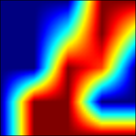
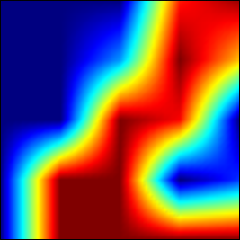
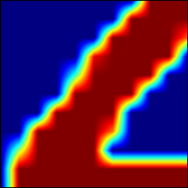
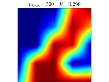
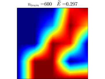
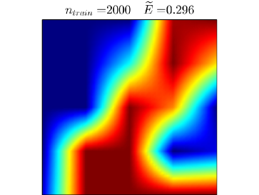
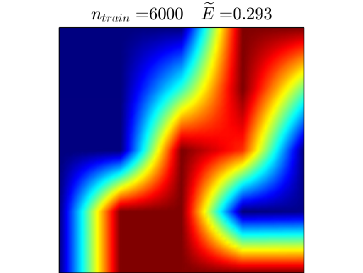
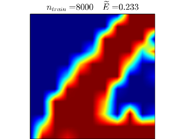
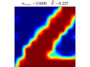
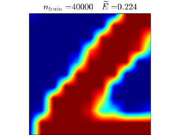
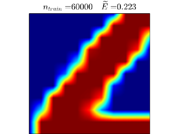
The solution of SOLO using 501 samples is presented in Fig. 2e, whose energy is 0.298, almost the same as that of the benchmark in Fig. 2d. With higher , the solution from SOLO becomes closer to that of the benchmark (the evolution of optimized structures is shown in Supplementary Fig. 2). In Fig. 2f, the energy is the same as the benchmark. The material distribution in Fig. 2f does not differ much from that in Fig. 2e. In fact, using only 501 samples is sufficient for the online training to find the optimized material distribution. We find that in our problem and optimization setting, the GSA needs about 2 function evaluations to obtain the minimum of DNN. Since the DNN approximates the objective function, we estimate GSA needs the same number of evaluations when applying to the objective, then it means 2 FEM calculations are required if directly using GSA. From this perspective, SOLO reduces the number of FEM calculations to 1/400.
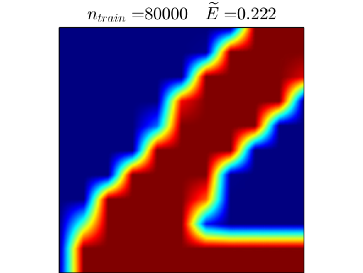
A similar problem with a finer mesh having 121 (1111) design variables is shown in Fig. 3a. The benchmark solution from MMA is shown in Fig. 3d, whose energy is 0.222. The trends in Fig. 3b and c are similar to those in Fig. 2 with a coarse mesh. Fig. 3b shows that SOLO converges at , giving . Our method again outperforms CMA-ES, the second best algorithm according to Fig. 2b. The material distribution solutions are shown in Fig. 3e and f. The configuration of SOLO is the same as that for the coarse mesh except that each loop has 1,000 incremental samples and GSA performs 4 function evaluations. Compared with directly using GSA, SOLO reduces the number of FEM calculations to 1/400 as well. The evolution of optimized structures is shown in Supplementary Fig. 3.
Fluid-structure optimization. In the following two problems, we leverage our algorithm to address binary fluid-structure optimization. We want to show that our method outperforms the gradient-based method and a recent algorithm based on reinforcement learning32.
 \SetHorizontalCoffin\labelcoffin
a\SetVerticalPole\imagecoffinleft3pt+\CoffinWidth\labelcoffin/2\SetVerticalPole\imagecoffinright\Width-3pt-\CoffinWidth\labelcoffin/2\SetHorizontalPole\imagecoffinup\Height-3pt-\CoffinHeight\labelcoffin/2\SetHorizontalPole\imagecoffindown3pt+\CoffinHeight\labelcoffin/2\JoinCoffins\imagecoffin[left,up]\labelcoffin[vc,hc]\TypesetCoffin\imagecoffin
 \SetHorizontalCoffin\labelcoffin
b\SetVerticalPole\imagecoffinleft3pt+\CoffinWidth\labelcoffin/2\SetVerticalPole\imagecoffinright\Width-3pt-\CoffinWidth\labelcoffin/2\SetHorizontalPole\imagecoffinup\Height-3pt-\CoffinHeight\labelcoffin/2\SetHorizontalPole\imagecoffindown3pt+\CoffinHeight\labelcoffin/2\JoinCoffins\imagecoffin[left,up]\labelcoffin[vc,hc]\TypesetCoffin\imagecoffin
c Gradient-based
d SOLO-G@286
e SOLO-R@2,148
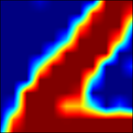
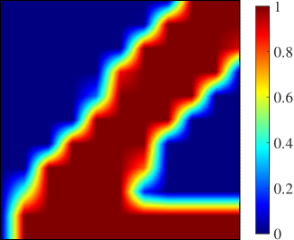
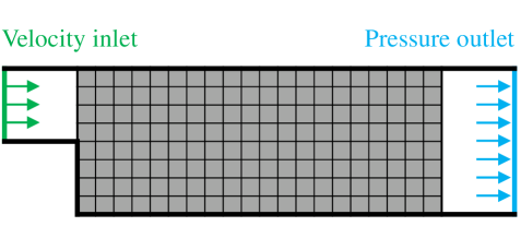
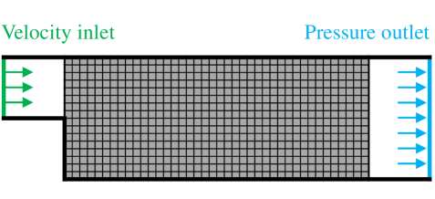
As shown in Fig. 4a, the fluid enters the left inlet at a given velocity perpendicular to the inlet, and flows through the channel bounded by walls to the outlet where the pressure is set as zero. In the mesh, we add solid blocks to change the flow field to minimize the friction loss when the fluid flows through the channel. Namely, we want to minimize the normalized inlet pressure
| (7) |
where denotes the average inlet pressure and indicates no solid in the domain. As for the fluid properties, we select a configuration with a low Reynolds number for stable steady solution 35, specifically,
| (8) |
where denotes fluid density, denotes viscosity, denotes inlet velocity and denotes inlet width (green line).
For the benchmark, we use a typical gradient-based algorithm which adds an impermeable medium to change binary variables to continuous ones 36. It uses the adjoint method to derive gradients and MMA as the solver. The solution is presented in Fig. 4c. The solid blocks form a ramp at the left bottom corner for a smooth flow expansion.
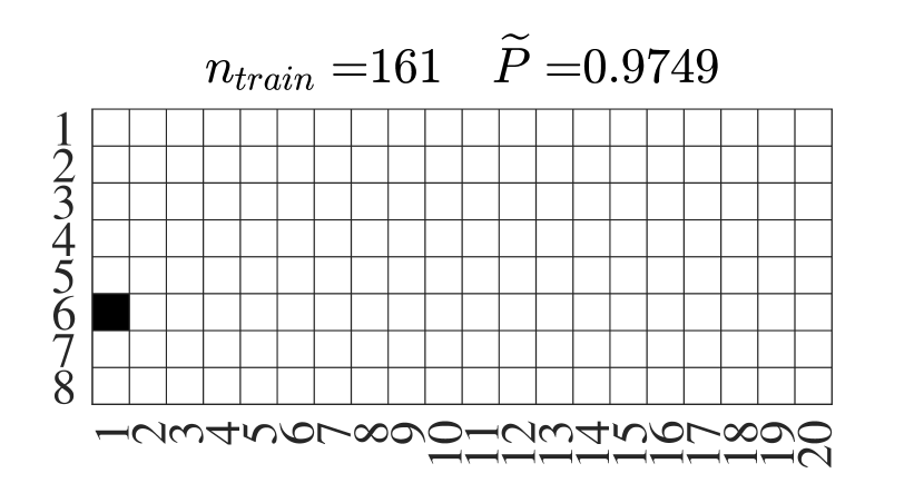
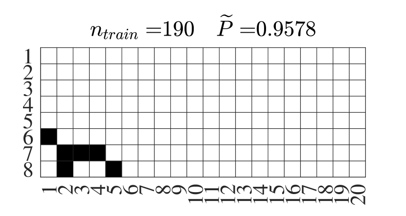
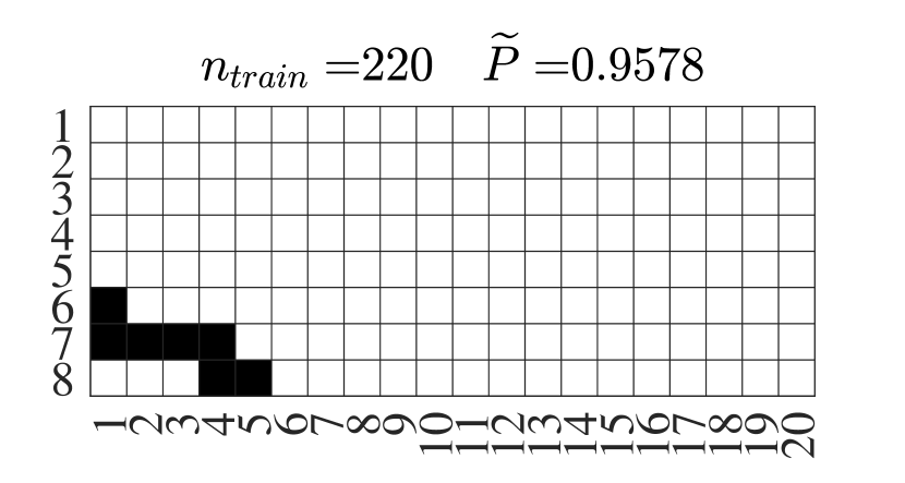
We use two variants of our algorithm. One is denoted as SOLO-G, a greedy version of SOLO where additional 10 samples produced in each loop are all from the DNN’s prediction. The initial batch is composed of a solution filled with zeros and 160 solutions each of which has a single element equal to one and others equal to zero. The pressure values corresponding to these designs are calculated by FEM. These 161 samples are used to train a DNN. Next, Binary Bat Algorithm (BBA) is used to find the minimum of the DNN. The top 10 solutions (after removing repeated ones) encountered during BBA searching will be used as the next batch of training data. The other variant, denoted as SOLO-R, is a regular version of SOLO where each loop has 100 incremental samples. 10 of them are produced in the same way as SOLO-G whereas the rest 90 are generated by adding disturbance to the best solution predicted by the DNN. Similar to the compliance minimization problems, the disturbance includes mutation and crossover.
 \SetHorizontalCoffin\labelcoffin
a\SetVerticalPole\imagecoffinleft3pt+\CoffinWidth\labelcoffin/2\SetVerticalPole\imagecoffinright\Width-3pt-\CoffinWidth\labelcoffin/2\SetHorizontalPole\imagecoffinup\Height-3pt-\CoffinHeight\labelcoffin/2\SetHorizontalPole\imagecoffindown3pt+\CoffinHeight\labelcoffin/2\JoinCoffins\imagecoffin[left,up]\labelcoffin[vc,hc]\TypesetCoffin\imagecoffin
 \SetHorizontalCoffin\labelcoffin
b\SetVerticalPole\imagecoffinleft3pt+\CoffinWidth\labelcoffin/2\SetVerticalPole\imagecoffinright\Width-3pt-\CoffinWidth\labelcoffin/2\SetHorizontalPole\imagecoffinup\Height-3pt-\CoffinHeight\labelcoffin/2\SetHorizontalPole\imagecoffindown3pt+\CoffinHeight\labelcoffin/2\JoinCoffins\imagecoffin[left,up]\labelcoffin[vc,hc]\TypesetCoffin\imagecoffin
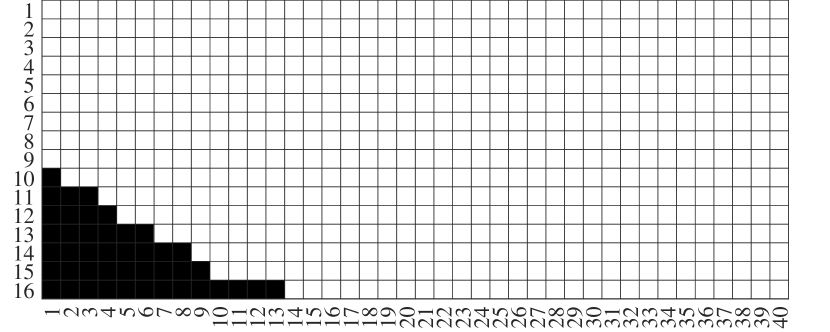
c Gradient-based
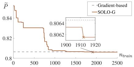
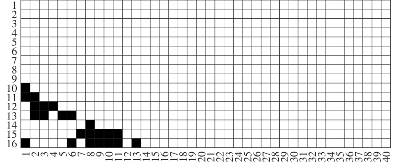
d SOLO-G@1,912
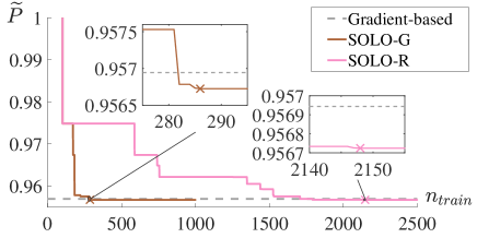
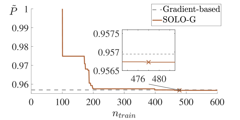
As shown in Fig. 4b, SOLO-G and SOLO-R converge to the same objective function value at and respectively. Their solutions are equivalent, shown in Fig. 4d and e. Intermediate solutions from SOLO-G are shown in Supplementary Fig. 4. We obtain the optimum better than the gradient-based method () after only 286 FEM calculations. For comparison, a recent topology optimization work based on reinforcement learning used the same geometry setup and obtained the same solution as the gradient-based method after thousands of iterations 32; our approach demonstrates better performance. Compared with directly using BBA which requires evaluations, SOLO-G reduces FEM calculations by orders of magnitude to about . To account for randomness, we repeat the experiments another four times and the results are similar to Fig. 4b (see Supplementary Figs. 5 and 6).
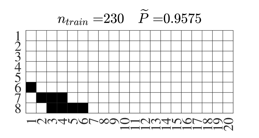
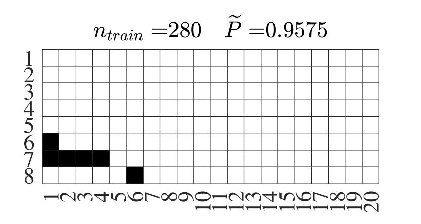
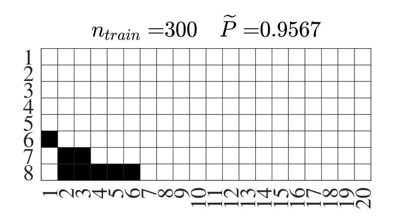
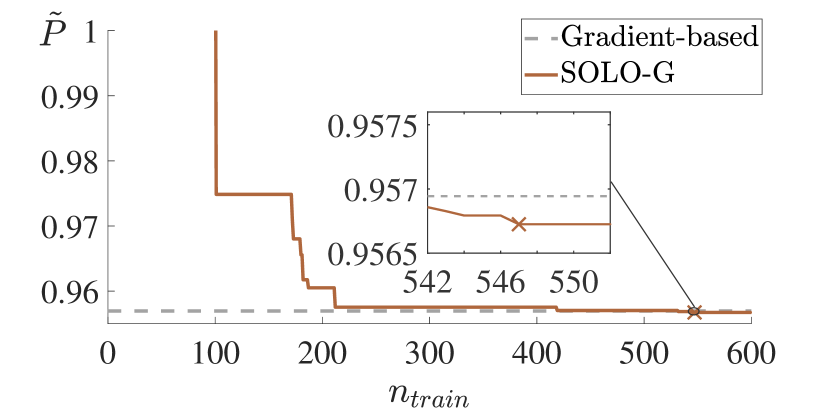
We also apply our algorithm to a finer mesh, with design variables (Fig. 5a). SOLO-G converges at , shown in Fig. 5b. Our design (Fig. 5d, ) is found to be better than the solution from the gradient-based algorithm (Fig. 5c, ). Intermediate solutions from SOLO-G are shown in Supplementary Fig. 7. Compared with directly using BBA which needs evaluations, SOLO-G reduces the number of FEM calculations to . Similar trends can be observed when repeating the experiments (see Supplementary Fig. 7). It is interesting to note that the optimum in Fig. 5d has two gaps at the 7th and 12th columns. It is a little counterintuitive, since the gradient-based method gives a smooth ramp (Fig. 5c). We try filling the gaps and find that their existence indeed reduces pressure (see Supplementary Fig. 8), which demonstrates how powerful our method is.
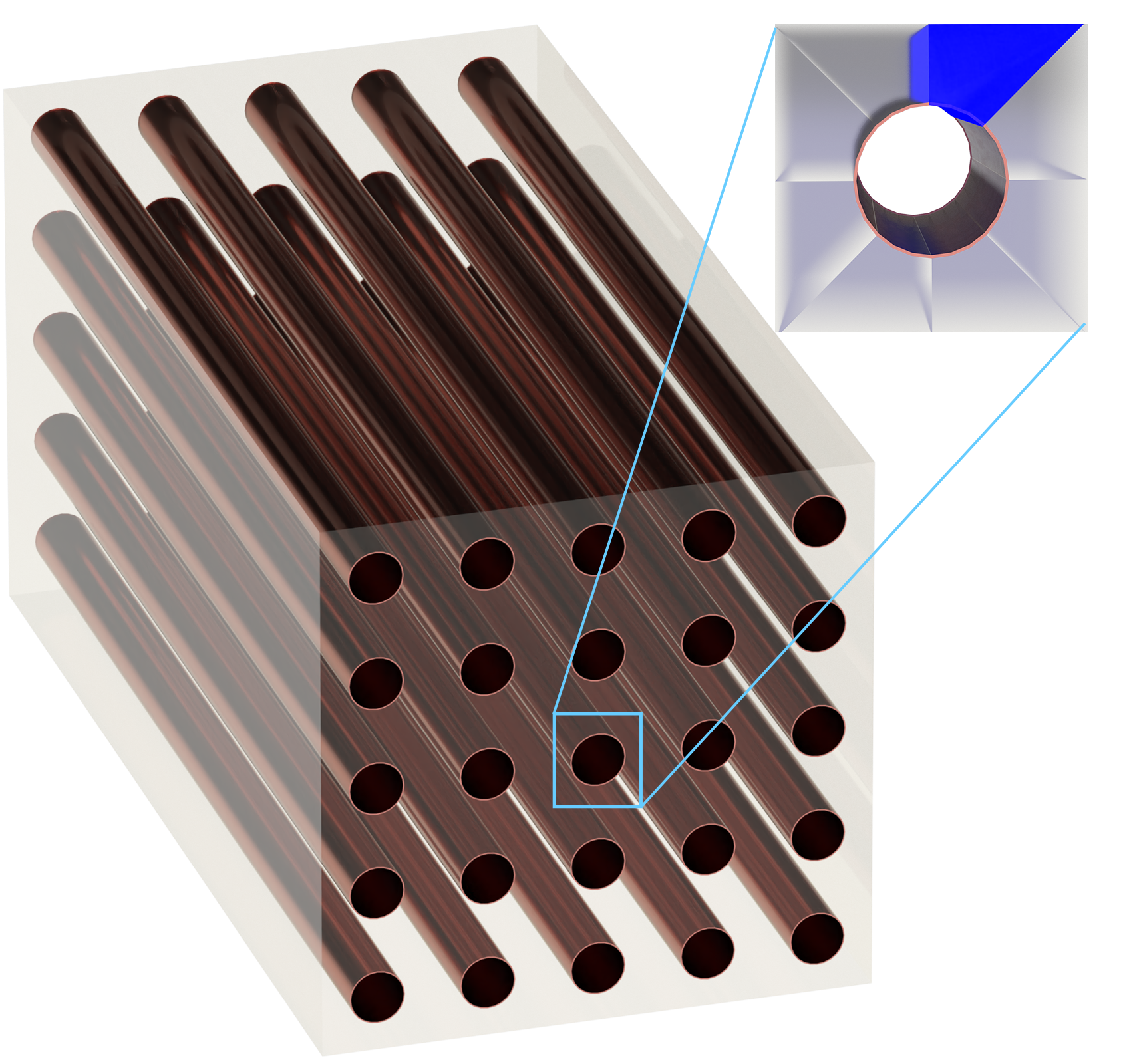
Heat transfer enhancement. In this example, we would like to solve a complicated problem that gradient-based methods are difficult to address. Phase change materials are used for energy storage by absorbing and releasing latent heat when the materials change phases, typically between solid and liquid. Due to their simple structure and high heat storage capacity, they are widely used in desalination, buildings, refrigeration, solar system, electronic cooling, spacecraft and so forth37. However, commonly used non-metallic materials suffer from very low thermal conductivity. A popular solution is to add high conductivity material (such as copper) as fins to enhance heat transfer 38. Topology optimization is implemented to optimize the geometry of fins. To deal with such transient problems, current gradient-based methods have to simplify the problem by using predetermined time period and fixed boundary conditions 39, 40, 41, 42. By contrast, in real applications, these conditions depend on user demand and environment, or even couple with the temperature field of the energy storage system 43, 44, 45, 46, 47. Therefore, problems with more complex settings need to be addressed.
 \SetHorizontalCoffin\labelcoffin
a\SetVerticalPole\imagecoffinleft3pt+\CoffinWidth\labelcoffin/2\SetVerticalPole\imagecoffinright\Width-3pt-\CoffinWidth\labelcoffin/2\SetHorizontalPole\imagecoffinup\Height-3pt-\CoffinHeight\labelcoffin/2\SetHorizontalPole\imagecoffindown3pt+\CoffinHeight\labelcoffin/2\JoinCoffins\imagecoffin[left,up]\labelcoffin[vc,hc]\TypesetCoffin\imagecoffin
 \SetHorizontalCoffin\labelcoffin
b\SetVerticalPole\imagecoffinleft3pt+\CoffinWidth\labelcoffin/2\SetVerticalPole\imagecoffinright\Width-3pt-\CoffinWidth\labelcoffin/2\SetHorizontalPole\imagecoffinup\Height-3pt-\CoffinHeight\labelcoffin/2\SetHorizontalPole\imagecoffindown3pt+\CoffinHeight\labelcoffin/2\JoinCoffins\imagecoffin[left,up]\labelcoffin[vc,hc]\TypesetCoffin\imagecoffin
 \SetHorizontalCoffin\labelcoffin
c\SetVerticalPole\imagecoffinleft3pt+\CoffinWidth\labelcoffin/2\SetVerticalPole\imagecoffinright\Width-3pt-\CoffinWidth\labelcoffin/2\SetHorizontalPole\imagecoffinup\Height-3pt-\CoffinHeight\labelcoffin/2\SetHorizontalPole\imagecoffindown3pt+\CoffinHeight\labelcoffin/2\JoinCoffins\imagecoffin[left,up]\labelcoffin[vc,hc]\TypesetCoffin\imagecoffin
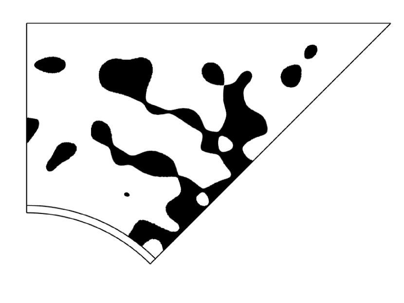
d SOLO@20,860

e Direct@24,644
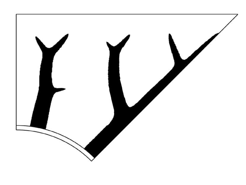
f Approximated
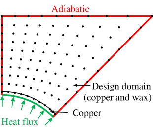
We consider a heat absorption scenario where time is variant and the boundary condition is coupled with the temperature field. As shown in Fig. 6a, copper pipes containing heat source are inserted in a phase change material, paraffin wax RT54HC 48; the heat source can be fast-charging batteries for electric vehicles or hot water for residential buildings. Considering symmetry, the problem is converted to a 2D problem in Fig. 6b. We fill the domain with wax to store heat and with copper to enhance heat transfer. The material distribution (1 being copper and 0 being wax) is represented by a 1010 mesh. Specifically, a continuous function is interpolated by Gaussian basis functions from the 1010 design variables and then converted to binary values by a threshold (see Methods for details). Our goal is to find the optimal to minimize the time to charge the system with a given amount of heat
| (9) |
where , means no copper inside the design domain, and is the time to charge the system with amount of heat, expressed by
| (10) |
subject to the maximum heat flux constraint at the boundary (green curve in Fig. 6b)
| (11) |
the constraint of maximum temperature of the domain,
| (12) |
and given copper usage, i.e., the volume constraint of copper,
| (13) |
Here , and are preset constants. Obviously, the bottom left boundary (inner side of copper pipes) has the highest temperature during charging, thus we only need to consider the temperature constraint at this boundary. Physically, there are one or two charging steps: the system is charged at heat flux until the boundary temperature reaches or the total heat flow reaches (whichever first), and if it is the former case, the heat flux is reduced to maintain the boundary temperature at until the total heat flow requirement is satisfied. In practice, we choose parameters such that the system will go through two steps for sure.
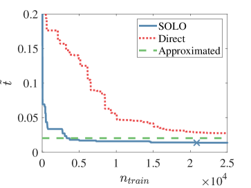
To solve the problem with objective Eq.(9) and constraints in Eqs.(11)-(13), our method SOLO is initialized by 500 random samples to train a DNN. Bat Algorithm (BA) is then used to find the minimum of the DNN, based on which additional 200 samples are generated in each loop by mutation and convolution. Two gradient-based methods are used as baselines to compare with our algorithm: one is to solve Problem (9)-(13) directly by gradient descent, denoted as “Direct”; the other is to simplify this problem to a steady state problem 42, denoted as “Approximated”. In Fig. 6c, SOLO converges at (marked by a cross “X”) with lower than other methods. It appears counter-intuitive that the solution of SOLO, shown in Fig. 6d, has some copper islands isolated from major branches. We tried removing these islands and adding more copper materials to the major branches to maintain copper volume, yet the variants showed worse performance, as shown in Supplementary Fig. 10. “Direct” gives the worst solution in Fig. 6e. “Approximated” yields a good solution with a tree structure, as shown in Fig. 6f; since it does not solve the same problem as the other two methods, we do not consider its relation with and represent it by a horizontal line in Fig. 6c.
Our method gives a good solution after 20,860 FEM calculations, while BA is estimated to need calculations. In summary, our method outperforms the other two methods and reduces the number of FEM calculations by over four orders of magnitude compared with BA.
Truss optimization. In this example, we test the scalability of SOLO with over a thousand design variables. Also, we will compare it with a heuristic method, BA, to provide direct evidence that SOLO can reduce the number of FEM computations by over two orders of magnitude.
 \SetHorizontalCoffin\labelcoffin
a\SetVerticalPole\imagecoffinleft3pt+\CoffinWidth\labelcoffin/2\SetVerticalPole\imagecoffinright\Width-3pt-\CoffinWidth\labelcoffin/2\SetHorizontalPole\imagecoffinup\Height-3pt-\CoffinHeight\labelcoffin/2\SetHorizontalPole\imagecoffindown3pt+\CoffinHeight\labelcoffin/2\JoinCoffins\imagecoffin[left,up]\labelcoffin[vc,hc]\TypesetCoffin\imagecoffin
 \SetHorizontalCoffin\labelcoffin
b\SetVerticalPole\imagecoffinleft3pt+\CoffinWidth\labelcoffin/2\SetVerticalPole\imagecoffinright\Width-3pt-\CoffinWidth\labelcoffin/2\SetHorizontalPole\imagecoffinup\Height-3pt-\CoffinHeight\labelcoffin/2\SetHorizontalPole\imagecoffindown3pt+\CoffinHeight\labelcoffin/2\JoinCoffins\imagecoffin[left,up]\labelcoffin[vc,hc]\TypesetCoffin\imagecoffin
c 72 bars
d 432 bars
e 1,008 bars
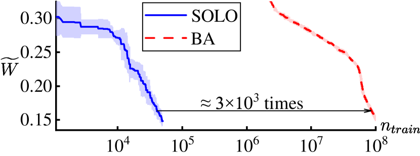
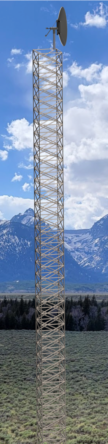
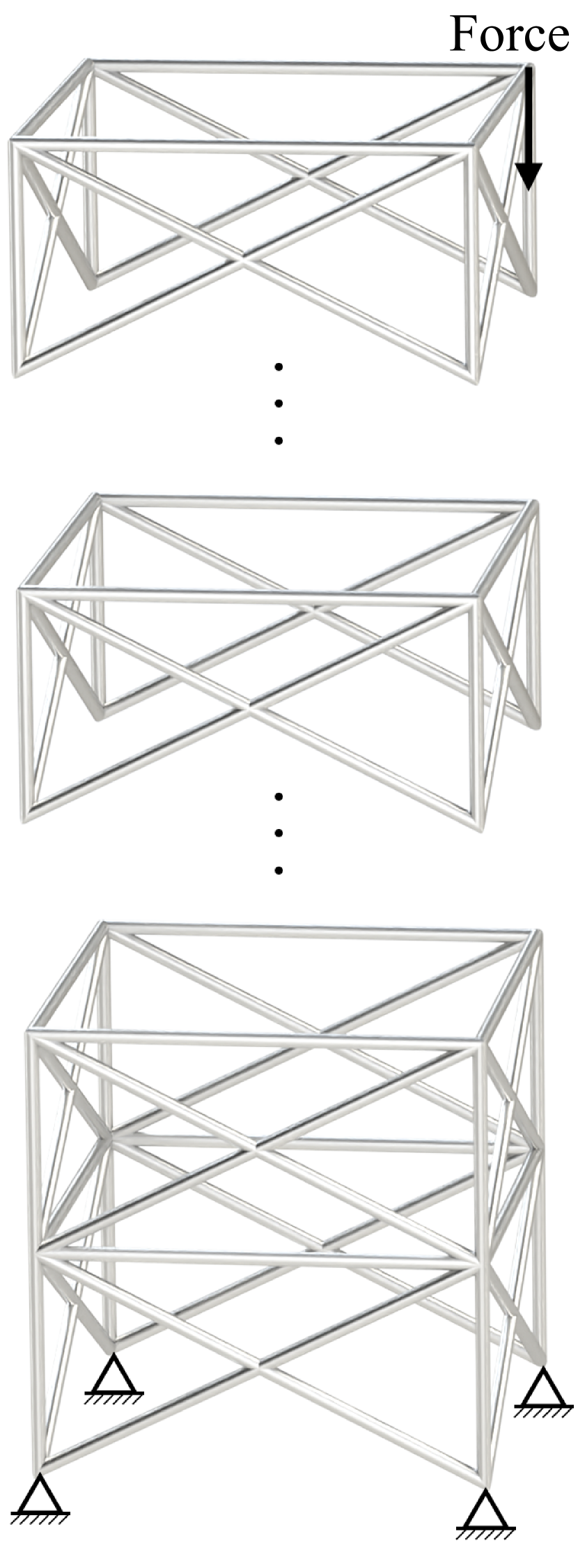
Truss structures are widely used in bridges, towers, buildings and so forth. An exemplary application, an antenna tower, is shown in Fig. 7a. Researchers have been working on optimizing truss structures from different perspectives. A classic truss optimization benchmark problem is to optimize a structure with 72 bars 49, 50, 51, 52, as shown in Fig. 7b with four repeated blocks, so as to minimize the weight of the bars subject to displacement and tension constraint. Following this benchmark problem, we set the goal to optimize the size of each bar (the bars can all have different sizes) to minimize total dimensionless weight
| (14) |
where , and are the cross-sectional area, length, and unit weight of the -th bar, respectively; uses the largest cross-sectional area for all bars; is the number of bars. Each bar is only allowed to choose from 16 discrete cross-sectional area values , to represent standardized components in engineering applications. The tension constraint requires all bars to not exceed the maximum stress
| (15) |
The displacement constraint is applied to the connections of the bars: the displacement in any direction is required to be lower than a threshold
| (16) |
where is the number of connections.
Now we have an optimization problem with objective Eq.(14) subject to stress constraint Eq.(15) and displacement constraint Eq.(16). In addition to the popular 72-bar problem, we add more repeated blocks to the structure to generate two more problems, with 432 and 1,008 bars. Geometric symmetry is not considered while solving the problems. Therefore, the design space goes up to , which is extremely huge. For the three problems, SOLO is initialized by 100, 500 and 1,000 samples, respectively. The number of incremental samples per loop is 10% of the initialization samples. 10% of incremental samples are the optima obtained by BA based on the DNN’s prediction, and the rest 90% are generated by mutation of the best solution predicted by the DNN.
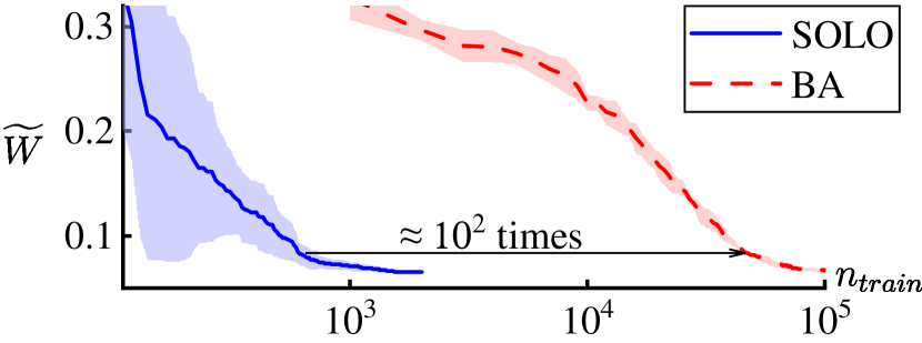
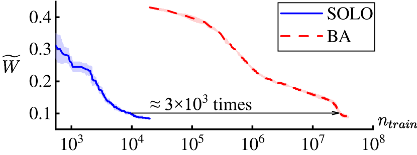
The results are shown in Fig. 7c-e. To reach the same objective weight, BA needs over times of calculations of SOLO. The difference becomes even larger when the number of variables increases. These examples demonstrate the scalability of SOLO by showing higher efficiency in computation, especially with a large number of design variables.
Discussion
Topology optimization is an important problem with broad applications in many scientific and engineering disciplines. Solving non-linear high-dimensional optimization problems requires non-gradient methods, but the high computational cost is a major challenge. We proposed an approach of self-directed online learning optimization (SOLO) to dramatically accelerate the optimization process and make solving complex optimization problems possible.
We demonstrated the effectiveness of the approach in solving eight problems of four types, i.e., two compliance minimization problems, two fluid-structure optimization problems, a heat transfer enhancement problem and three truss optimization problems. For the compliance problems with 25 and 121 continuous design variables, our approach converged and produced optimized solutions same as the known optima with only 501 and 10,243 FEM calculations, respectively, which are about 1/400 of directly using GSA and FEM without DNN based on our estimation. For the fluid problems with 160 and 640 binary variables, our method (SOLO-G) converged after 286 and 1,912 FEM calculations, respectively, with solutions better than the benchmark. It used less than of FEM calculations compared with directly applying BBA to FEM, and converged much faster than another work based on reinforcement learning. In the heat transfer enhancement example, we investigated a complicated, transient and non-linear problem. Our method gave a solution that outperformed other baselines after 20,860 FEM calculations, which was estimated to be four orders of magnitude less than BA. Similar to other SMBO methods, overhead computation was introduced (by training DNNs and finding their optima), but it was almost negligible (see the time profile in Supplementary Table 1) which is attractive for real-world applications where new designs want to be developed and tested. In these examples, we estimated the amount of computation of directly using heuristic algorithms, which showed that our approach led to orders of magnitude of computation reduction. In addition to this estimation, we applied BA to the original objectives in the three truss optimization problems and observed orders of magnitude of calculation reduction using our approach.
Our algorithm is neat and efficient, and has great potential for large-scale applications. We bring a new perspective for high-dimensional optimization by embedding deep learning in optimization methods. More techniques, such as parallel FEM computation, uncertainty modeling and disturbance based on sensitivity analysis, can be incorporated to enhance the performance.
Methods
Enforcement of volume constraint. Compliance and heat transfer problems have volume constraints. The latter will be detailed in Section Interpolation of design variables, thus we only discuss the former here. In the two compliance problems, all matrices representing the density distribution have the same weighted average due to the volume constraint where denotes the weight of linear Gaussian quadrature. A matrix from the initial batch is generated by three steps:
-
1.
Generate a random matrix with elements uniformly distributed from 0 to 1.
-
2.
Rescale the array to enforce the predefined weighted average.
-
3.
Set the elements greater than one, if any, to one and then adjust those elements less than one to maintain the average.
Matrices for the second batch and afterwards add random disturbance to optimized solutions and then go through Step 2 and 3 above to make sure the volume satisfies the constraint.
Finite Element Method (FEM) and gradient-based baselines. The objective function values of material designs are calculated by FEM as the ground truth to train the DNN. In the compliance and fluid problems, the meshes of FEM are the same as the design variables. In the heat problem, the meshes are finer. Numerical results are obtained by COMSOL Multiphysics 5.4 (except the truss problems). Solutions from gradient-based methods (including “Approximated” ) are all solved by MMA via COMSOL with optimality tolerance as 0.001. In the fluid problems, the gradient-based baseline method produces a continuous array, and we use multiple thresholds to convert it to binary arrays and recompute their objective (pressure) to select the best binary array. In the heat problem, the “Approximated” method uses the same resolution as the other two methods (SOLO and “Direct”) for a fair comparison. Specifically, we apply a Helmholtz filter53, whose radius is half of the minimum distance of two design variable locations, to yield a mesh-independent solution. The solution is a continuous array; we use a threshold to convert it to a binary array which satisfies the volume constraint in Eq.(14).
Interpolation of design variables. In the two compliance problems and the heat problem, we use a vector (or matrix) to represent a spacial function . Interpolation is needed to obtain the function for FEM and plotting. Given design variables , we get the values by two interpolation methods. For the compliance problems, we use bilinear interpolation54. Suppose is within a rectangular element whose nodal coordinates are , the interpolated function value can be calculated by
| (17) |
For the heat problem, a continuous function (which will later be converted to a binary function which takes 0 or 1) is interpolated by Gaussian basis functions 13, 20:
| (18) |
where ( is a preset distance), and are parameters to be determined. The following constraints are needed to guarantee a unique solution
| (19) |
Expressing the above equations by a matrix form, we have
| (20) |
abbreviated as . We get and interpolate by Eq.(18). Then we set a threshold to convert the continuous function to a binary one , i.e., if and otherwise. The threshold is controlled to satisfy the copper volume constraint Eq.(13).
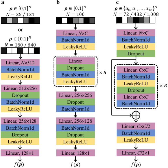
Deep Neural Network (DNN). The architectures of the DNN used in this paper is presented in Fig. 8. The design variable is flattened to a 1D vector as the input to DNN. All inputs are normalized before training and we introduce batch normalization (BN)55 within the network as regularization. The output of DNN is reciprocal of the objective function (energy, pressure, charging time or weight) to give better resolution at lower objective values. For the rest of this paper, we regard the DNN to approximate the objective function for simplicity. To optimize the DNN training process, we apply ADAM56 as the optimizer implemented on the platform of PyTorch 1.8.057. The learning rate is 0.01. The loss function is set as Mean Square Error (MSE)58. All models are trained for 1,000 epochs with a batch size of 1,024 (if the number of training data is less than 1,024, all the data will be used as one batch).
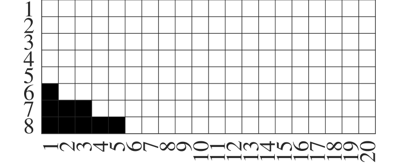
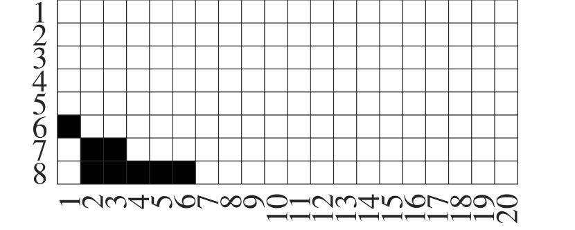
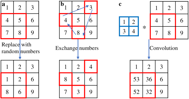
Random generation of new samples from a base design. After calculating the optimized array , more training data are generated by adding disturbance to it. As shown in Fig. 9, there are three kinds of disturbance: mutation, crossover and convolution. They are all likely to change the weighted average of an array, thus the enforcement of volume constraint will be applied when necessary. Mutation means mutating several adjacent cells in the optimized array, i.e., generating random numbers from 0 to 1 to replace the original elements. In the 2D example shown in Fig. 9a, the numbers in a 2-by-2 box are set as random. Crossover denotes the crossover of cells in the array and is achieved by the following steps:
-
1.
Assign a linear index to each element in the array.
-
2.
Randomly pick several indices.
-
3.
Generate a random sequence of the indices.
-
4.
Replace the original numbers according to the sequence above. As shown in Fig. 9b, indices are assigned sequentially from left to right and from top to bottom. The indices we pick in Step 2 are 3, 4 and 8; the sequence generated in Step 3 is 4, 8 and 3.
In the two compliance problems, the ways to generate a new input matrix based on and their possibilities are:
-
(a)
mutation: mutating one element in (10%);
-
(b)
mutation: mutating a 22 matrix in (10%);
-
(c)
mutation: mutating a 33 matrix in (20%);
-
(d)
mutation: mutating a 44 matrix in (20%);
-
(e)
crossover: choosing an integer from one to the number of total elements, selecting cells in and permuting them (20%);
-
(f)
generating a completely random matrix like the initial batch (20%).
In the fluid problem with mesh, i.e. SOLO-R, the ways are the same as previous ones except a threshold is needed to convert the continuous array into a binary one. The threshold has 50% probability to be where is uniformly sampled from , and has 50% probability to be the element-wise mean of . In the heat problem, crossover is replaced by convolution. It is the same as the compliance problems except that (e) above is replaced by
-
(g)
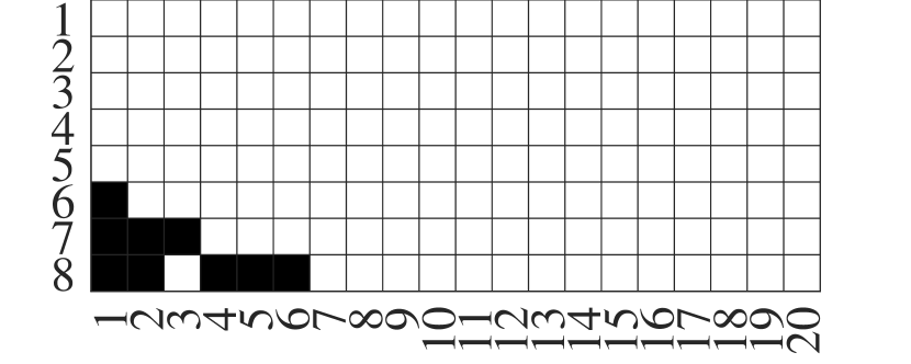
Convolution: substituting a submatrix of the array, whose size and the corresponding probability is the same as (a-d), with a same convolution (the output has the same size as the input submatrix) between the submatrix and kernel whose element is uniformly sampled from .
In the truss optimization problems, the design variable is purely one-dimensional and can no longer be represented as a matrix. Therefore, we only use mutation. First, is uniformly sampled from to indicate the ratio of elements to be mutated in , and then those elements are randomly selected to add to themselves; is uniformly sampled from .
Generalized Simulated Annealing (GSA). Simulated Annealing (SA) is a stochastic method to determine the global minimum of a objective function by simulating the annealing process of a molten metal 60. GSA is a type of SA with specific forms of visiting function and acceptance probability61. Assuming objective
| (21) |
we do the following:
-
1.
Generate an initial state randomly and obtain its function value . Set parameters , , , .
-
2.
For artificial time step to ,
-
(a)
Generate a new state , where the probability distribution of follows the visiting function
(22) where denotes the artificial temperature calculated by
(23) -
(b)
Calculate the energy difference
(24) -
(c)
Calculate the probability to accept the new state
(25) Determine whether to accept the new state based on the probability, if not, .
-
(a)
-
3.
Conduct local search to refine the state.
Since compliance minimization has a volume constraint, the objective function used in the optimization process is written as
| (26) |
where is a constant to transform the constrained problem to an unconstrained problem by adding a penalty term. GSA is implemented via SciPy package with default parameter setting. For more details please refer to its documentation62.
Bat Algorithm (BA). Bat Algorithm (BA) is a heuristic optimization algorithm, inspired by the echolocative behavior of bats 63. This algorithm carries out the search process using artificial bats mimicking the natural pulse loudness, emission frequency and velocity of real bats. It solves the problem
| (27) |
We adopt a modification 64 and implement as follows:
-
1.
Generate vectors . We use to denote a vector, flattened from the array representing design variables. It is treated as the position of the -th artificial bat, where . We use to denote the -th dimension of vector , where . Thus, .
-
2.
Calculate their function values and find the minimum .
-
3.
Initialize their velocity .
-
4.
Determine parameters , , , , , , , , .
-
5.
For artificial time step to ,
-
(a)
Update parameters , , .
-
(b)
For ,
-
i.
Calculate sound frequency
(28) where is a random number that has a uniform distribution in .
-
ii.
Update velocity based on frequency
(29) -
iii.
Get a (temporary) new solution. Calculate the new position
(30) -
iv.
Local search. Generate , a series of random numbers uniformly sampled in . For those satisfying , add noise to current best solution
(31) where is a random variable sampled in Gaussian distribution with zero mean, is the -th component of . If goes over the range , it is thresholded to 0 or 1. For others, keep them as they are.
-
v.
Determine whether to accept the new solution. Reverse to the previous step , if or (where is random number uniformly sampled in ).
-
i.
-
(c)
Update .
-
(a)
-
6.
Output .
BA is used in the heat and truss problems. In the heat problem, we optimize without adding penalty terms since the volume constraint is controlled by a threshold, i.e., . In the truss optimization problems, we need to choose in a discrete space since only 16 values are allowed. Before we evaluate , we will replace by the nearest discrete values. To deal with constraints in Eqs. (15) and (16), the objective function is converted to
| (32) |
Binary Bat Algorithm (BBA). Binary Bat Algorithm 65, 66 is a binary version of BA. To solve
| (33) |
we slightly adjust the original algorithm and implement it as follows:
-
1.
Generate vectors . We use to denote a vector, flattened from the array representing design variables. It is treated as the position of the -th artificial bat, where . We use to denote the -th dimension of vector , where . Thus, .
-
2.
Calculate their function values and find the minimum .
-
3.
Initialize their velocity .
-
4.
Determine parameters , , , , , , .
-
5.
For artificial time step to ,
-
(a)
Update parameters , .
-
(b)
For ,
-
i.
Calculate sound frequency
(34) where is a random number that has a uniform distribution in .
-
ii.
Update velocity based on frequency
(35) -
iii.
Get a (temporary) new solution. Calculate the possibility to change position based on velocity
(36) -
iv.
Random flip. Generate , a series of random numbers uniformly in [0,1]. For those satisfying , change the position by flipping the 0/1 values
(37) For others, keep them as they are.
-
v.
Accept the local optimum. Generate , a series of random numbers uniformly sampled in . For those satisfying , set .
-
vi.
Determine whether to accept the new solution. Reverse to the previous step , if or (where is random number uniformly sampled in [0,1]).
-
i.
-
(c)
Update .
-
(a)
-
6.
Output .
BBA is used in the fluid problems. Since we do not have constraints in these problems, we can optimize without adding penalty terms, i.e., .
Data availability
The optimization data generated in this study have been deposited in the Zenodo database 67.
Code availability
All code (MATLAB and Python) used in this paper is deposited in the Zenodo repository 68 or available at https://github.com/deng-cy/deep_learning_topology_opt.
References
- 1 Deaton, J. D. & Grandhi, R. V. A survey of structural and multidisciplinary continuum topology optimization: post 2000. Structural and Multidisciplinary Optimization 49, 1–38 (2014).
- 2 Bendsøe, M. P. & Kikuchi, N. Generating optimal topologies in structural design using a homogenization method. Computer Methods in Applied Mechanics and Engineering 71, 197–224 (1988).
- 3 Rozvany, G. I. A critical review of established methods of structural topology optimization. Structural and multidisciplinary optimization 37, 217–237 (2009).
- 4 Sigmund, O. & Maute, K. Topology optimization approaches. Structural and Multidisciplinary Optimization 48, 1031–1055 (2013).
- 5 Sigmund, O. On the usefulness of non-gradient approaches in topology optimization. Structural and Multidisciplinary Optimization 43, 589–596 (2011).
- 6 Hajela, P. & Lee, E. Genetic algorithms in truss topological optimization. International Journal of Solids and Structures 32, 3341–3357 (1995).
- 7 Shim, P. Y. & Manoochehri, S. Generating optimal configurations in structural design using simulated annealing. International journal for numerical methods in engineering 40, 1053–1069 (1997).
- 8 Kaveh, A., Hassani, B., Shojaee, S. & Tavakkoli, S. Structural topology optimization using ant colony methodology. Engineering Structures 30, 2559–2565 (2008).
- 9 Luh, G.-C. & Lin, C.-Y. Structural topology optimization using ant colony optimization algorithm. Applied Soft Computing 9, 1343–1353 (2009).
- 10 Luh, G.-C., Lin, C.-Y. & Lin, Y.-S. A binary particle swarm optimization for continuum structural topology optimization. Applied Soft Computing 11, 2833–2844 (2011).
- 11 Lee, K. S. & Geem, Z. W. A new structural optimization method based on the harmony search algorithm. Computers & Structures 82, 781–798 (2004).
- 12 Georgiou, G., Vio, G. A. & Cooper, J. E. Aeroelastic tailoring and scaling using Bacterial Foraging Optimisation. Structural and Multidisciplinary Optimization 50, 81–99 (2014).
- 13 Guirguis, D., Melek, W. W. & Aly, M. F. High-resolution non-gradient topology optimization. Journal of Computational Physics 372, 107–125 (2018).
- 14 Guirguis, D. & Aly, M. F. A derivative-free level-set method for topology optimization. Finite Elements in Analysis and Design 120, 41–56 (2016).
- 15 Bartz-Beielstein, T. A survey of model-based methods for global optimization. Bioinspired Optimization Methods and Their Applications 1–18 (2016).
- 16 Hutter, F., Hoos, H. H. & Leyton-Brown, K. Sequential model-based optimization for general algorithm configuration. In International conference on learning and intelligent optimization, 507–523 (Springer, 2011).
- 17 Frazier, P. I. A tutorial on bayesian optimization. arXiv preprint arXiv:1807.02811 (2018).
- 18 Hansen, N. The cma evolution strategy: A tutorial. arXiv preprint arXiv:1604.00772 (2016).
- 19 Bujny, M., Aulig, N., Olhofer, M. & Duddeck, F. Hybrid evolutionary approach for level set topology optimization. In 2016 IEEE Congress on Evolutionary Computation (CEC), 5092–5099 (IEEE, 2016).
- 20 Luo, Y., Xing, J. & Kang, Z. Topology optimization using material-field series expansion and kriging-based algorithm: An effective non-gradient method. Computer Methods in Applied Mechanics and Engineering 364, 112966 (2020).
- 21 Jin, J., Yang, C. & Zhang, Y. An improved cma-es for solving large scale optimization problem. In International Conference on Swarm Intelligence, 386–396 (Springer, 2020).
- 22 Wang, Z., Hutter, F., Zoghi, M., Matheson, D. & de Feitas, N. Bayesian optimization in a billion dimensions via random embeddings. Journal of Artificial Intelligence Research 55, 361–387 (2016).
- 23 Lei, X., Liu, C., Du, Z., Zhang, W. & Guo, X. Machine Learning Driven Real Time Topology Optimization under Moving Morphable Component (MMC)-Based Framework. Journal of Applied Mechanics 86, 011004 (2018).
- 24 Banga, S., Gehani, H., Bhilare, S., Patel, S. & Kara, L. 3d topology optimization using convolutional neural networks. arXiv preprint arXiv:1808.07440 (2018).
- 25 Oh, S., Jung, Y., Kim, S., Lee, I. & Kang, N. Deep Generative Design: Integration of Topology Optimization and Generative Models. Journal of Mechanical Design 1–22 (2019).
- 26 Sosnovik, I. & Oseledets, I. Neural networks for topology optimization. Russian Journal of Numerical Analysis and Mathematical Modelling 34, 215–223 (2019).
- 27 Rawat, S. & Shen, M.-H. H. A novel topology optimization approach using conditional deep learning. arXiv preprint arXiv:1901.04859 (2019).
- 28 Jang, S., Yoo, S. & Kang, N. Generative design by reinforcement learning: enhancing the diversity of topology optimization designs. arXiv preprint arXiv:2008.07119 (2020).
- 29 Shen, M.-H. H. & Chen, L. A new cgan technique for constrained topology design optimization. arXiv preprint arXiv:1901.07675 (2019).
- 30 Yu, Y., Hur, T., Jung, J. & Jang, I. G. Deep learning for determining a near-optimal topological design without any iteration. Structural and Multidisciplinary Optimization 59, 787–799 (2019). 1801.05463.
- 31 Sasaki, H. & Igarashi, H. Topology optimization accelerated by deep learning. IEEE Transactions on Magnetics 55, 1–5 (2019).
- 32 Gaymann, A. & Montomoli, F. Deep neural network and monte carlo tree search applied to fluid-structure topology optimization. Scientific reports 9, 1–16 (2019).
- 33 Whitley, D. A genetic algorithm tutorial. Statistics and Computing 4, 65–85 (1994).
- 34 Bendsoe, M. P. & Sigmund, O. Topology Optimization: Theory, Methods and Applications (Springer, 2004).
- 35 Deng, C., Qi, X. & Liu, Y. Numerical study on equilibrium stability of objects in fluid flow—a case study on constructal law. Case Studies in Thermal Engineering 15, 100539 (2019).
- 36 Olesen, L. H., Okkels, F. & Bruus, H. A high-level programming-language implementation of topology optimization applied to steady-state navier–stokes flow. International Journal for Numerical Methods in Engineering 65, 975–1001 (2006).
- 37 Kamkari, B. & Shokouhmand, H. Experimental investigation of phase change material melting in rectangular enclosures with horizontal partial fins. International Journal of Heat and Mass Transfer 78, 839–851 (2014).
- 38 Desai, A. N., Gunjal, A. & Singh, V. Numerical investigations of fin efficacy for phase change material (pcm) based thermal control module. International Journal of Heat and Mass Transfer 147, 118855 (2020).
- 39 Chen, J., Xia, B. & Zhao, C. Topology optimization for heat transfer enhancement in thermochemical heat storage. International Journal of Heat and Mass Transfer 154, 119785 (2020).
- 40 Pizzolato, A., Sharma, A., Maute, K., Sciacovelli, A. & Verda, V. Topology optimization for heat transfer enhancement in latent heat thermal energy storage. International Journal of Heat and Mass Transfer 113, 875–888 (2017).
- 41 Iradukunda, A.-C., Vargas, A., Huitink, D. & Lohan, D. Transient thermal performance using phase change material integrated topology optimized heat sinks. Applied Thermal Engineering 179, 115723 (2020).
- 42 Zhao, M., Tian, Y., Hu, M., Zhang, F. & Yang, M. Topology optimization of fins for energy storage tank with phase change material. Numerical Heat Transfer, Part A: Applications 77, 284–301 (2020).
- 43 Li, Y. et al. Optimization of thermal management system for li-ion batteries using phase change material. Applied Thermal Engineering 131, 766–778 (2018).
- 44 Weng, J. et al. Optimization of the detailed factors in a phase-change-material module for battery thermal management. International Journal of Heat and Mass Transfer 138, 126–134 (2019).
- 45 Yan, J., Li, K., Chen, H., Wang, Q. & Sun, J. Experimental study on the application of phase change material in the dynamic cycling of battery pack system. Energy Conversion and Management 128, 12–19 (2016).
- 46 Arıcı, M., Bilgin, F., Nižetić, S. & Karabay, H. Pcm integrated to external building walls: An optimization study on maximum activation of latent heat. Applied Thermal Engineering 165, 114560 (2020).
- 47 Xu, T., Humire, E. N., Chiu, J. N.-W. & Sawalha, S. Numerical thermal performance investigation of a latent heat storage prototype toward effective use in residential heating systems. Applied Energy 278, 115631 (2020).
- 48 Yu, J. et al. Effect of porous media on the heat transfer enhancement for a thermal energy storage unit. Energy Procedia 152, 984–989 (2018).
- 49 Gomes, H. M. Truss optimization with dynamic constraints using a particle swarm algorithm. Expert Systems with Applications 38, 957–968 (2011).
- 50 Farshchin, M., Camp, C. & Maniat, M. Multi-class teaching–learning-based optimization for truss design with frequency constraints. Engineering Structures 106, 355–369 (2016).
- 51 Perez, R. l. & Behdinan, K. Particle swarm approach for structural design optimization. Computers & Structures 85, 1579–1588 (2007).
- 52 Camp, C. V. & Farshchin, M. Design of space trusses using modified teaching–learning based optimization. Engineering Structures 62, 87–97 (2014).
- 53 Lazarov, B. S. & Sigmund, O. Filters in topology optimization based on helmholtz-type differential equations. International Journal for Numerical Methods in Engineering 86, 765–781 (2011).
- 54 Han, D. Comparison of commonly used image interpolation methods. In Proceedings of the 2nd International Conference on Computer Science and Electronics Engineering (ICCSEE 2013), vol. 10 (2013).
- 55 Ioffe, S. & Szegedy, C. Batch normalization: Accelerating deep network training by reducing internal covariate shift. In International conference on machine learning, 448–456 (PMLR, 2015).
- 56 Kingma, D. P. & Ba, J. Adam: A method for stochastic optimization. arXiv preprint arXiv:1412.6980 (2014).
- 57 Paszke, A. et al. Automatic differentiation in pytorch. In NIPS-W (2017).
- 58 Lehmann, E. & Casella, G. Theory of Point Estimation (Springer Verlag, 1998).
- 59 Srivastava, N., Hinton, G., Krizhevsky, A., Sutskever, I. & Salakhutdinov, R. Dropout: A simple way to prevent neural networks from overfitting. Journal of Machine Learning Research 15, 1929–1958 (2014).
- 60 Xiang, Y., Gubian, S. & Martin, F. Generalized simulated annealing. In Peyvandi, H. (ed.) Computational Optimization in Engineering, chap. 2 (IntechOpen, Rijeka, 2017). URL https://doi.org/10.5772/66071.
- 61 Xiang, Y., Gubian, S., Suomela, B. & Hoeng, J. Generalized Simulated Annealing for Global Optimization: The GenSA Package. The R Journal 5, 13 (2013).
- 62 The SciPy community. scipy.optimize.dual_annealing – scipy v1.3.0 reference guide. https://docs.scipy.org/doc/scipy/reference/generated/scipy.optimize.dual_annealing.html (2019). Accessed: 2019-05-19.
- 63 Yang, X.-S. A new metaheuristic bat-inspired algorithm. In Nature inspired cooperative strategies for optimization (NICSO 2010), 65–74 (Springer, 2010).
- 64 Yılmaz, S. & Küçüksille, E. U. A new modification approach on bat algorithm for solving optimization problems. Applied Soft Computing 28, 259–275 (2015).
- 65 Mirjalili, S., Mirjalili, S. M. & Yang, X.-S. Binary bat algorithm. Neural Computing and Applications 25, 663–681 (2014).
- 66 Ramasamy, R. & Rani, S. Modified binary bat algorithm for feature selection in unsupervised learning. Int. Arab J. Inf. Technol. 15, 1060–1067 (2018).
- 67 Deng, C., Wang, Y., Qin, C., Fu, Y. & Lu, W. Self-Directed Online Machine Learning for Topology Optimization. Zenodo. https://doi.org/10.5281/zenodo.5725598 (2021).
- 68 Deng, C., Wang, Y., Qin, C., Fu, Y. & Lu, W. Self-Directed Online Machine Learning for Topology Optimization. Zenodo. https://doi.org/10.5281/zenodo.5722376 (2021).
- 69 Nair, V. & Hinton, G. E. Rectified linear units improve restricted boltzmann machines. In ICML (2010).
- 70 Bartlett, P. L., Foster, D. J. & Telgarsky, M. J. Spectrally-normalized margin bounds for neural networks. In Advances in Neural Information Processing Systems, 6240–6249 (2017).
- 71 Neyshabur, B., Bhojanapalli, S. & Srebro, N. A pac-bayesian approach to spectrally-normalized margin bounds for neural networks. arXiv preprint arXiv:1707.09564 (2017).
- 72 Chen, M., Li, X. & Zhao, T. On generalization bounds of a family of recurrent neural networks. arXiv preprint arXiv:1910.12947 (2019).
- 73 Blair, C. Problem complexity and method efficiency in optimization (as nemirovsky and db yudin). SIAM Review 27, 264 (1985).
- 74 Nemirovski, A., Juditsky, A., Lan, G. & Shapiro, A. Robust stochastic approximation approach to stochastic programming. SIAM Journal on optimization 19, 1574–1609 (2009).
- 75 Lin, T., Jin, C. & Jordan, M. I. On gradient descent ascent for nonconvex-concave minimax problems. arXiv preprint arXiv:1906.00331 (2019).
- 76 Chen, M. et al. On computation and generalization of generative adversarial imitation learning. arXiv preprint arXiv:2001.02792 (2020).
- 77 McDiarmid, C. Concentration. In Probabilistic methods for algorithmic discrete mathematics, 195–248 (Springer, 1998).
- 78 Mohri, M., Rostamizadeh, A. & Talwalkar, A. Foundations of machine learning (MIT press, 2018).
- 79 Bartlett, P. L. & Mendelson, S. Rademacher and gaussian complexities: Risk bounds and structural results. Journal of Machine Learning Research 3, 463–482 (2002).
Acknowledgement
The authors gratefully acknowledge the support by the National Science Foundation under Grant No. CNS-1446117 (W.L.).
Competing interests
The authors declare no conflict of interests.
Author contributions
C.D. designed the algorithm and drafted the manuscript. Y.W. derived the convergence theory. C.D. and C.Q. wrote the code. Y.W., C.Q. and Y.F. edited the manuscript. W.L. supervised this study and revised the manuscript.
Supplementary Information
Table of Contents
Section 1: Supplementary table and figures 1
- •
- •
- •
- •
- •
- •
- •
- •
- •
- •
- •
Section 2: Theory on convergence 2
-
•
Section 2.1: Formulation and theorem 2.1
-
•
Section 2.2: Preliminaries 2.2
- •
1 Supplementary table and figures
| Problem | Number of | Wall time /s | ||
| additional samples | FEM | Training | Optimization (evaluations) | |
| Compliance 55 | 100 | 40 | 35 | 70 () |
| Compliance 1111 | 1000 | 500 | 150 | 1000 () |
| Fluid 208 (G) | 10 | 35 | 10 | 35 () |
| Fluid 208 (R) | 100 | 350 | 20 | 35 () |
| Fluid 4016 (G) | 10 | 60 | 25 | 140 () |
| Heat 1010 | 200 | 40000 | 25 | 200 () |
| Truss 72 | 10 | 0.02 | 20 | 300 () |
| Truss 432 | 50 | 0.05 | 150 | 500 () |
| Truss 1008 | 100 | 0.15 | 1500 | 1500 () |
 \SetHorizontalCoffin\labelcoffin
a\SetVerticalPole\imagecoffinleft3pt+\CoffinWidth\labelcoffin/2\SetVerticalPole\imagecoffinright\Width-3pt-\CoffinWidth\labelcoffin/2\SetHorizontalPole\imagecoffinup\Height-3pt-\CoffinHeight\labelcoffin/2\SetHorizontalPole\imagecoffindown3pt+\CoffinHeight\labelcoffin/2\JoinCoffins\imagecoffin[left,up]\labelcoffin[vc,hc]\TypesetCoffin\imagecoffin
 \SetHorizontalCoffin\labelcoffin
b\SetVerticalPole\imagecoffinleft3pt+\CoffinWidth\labelcoffin/2\SetVerticalPole\imagecoffinright\Width-3pt-\CoffinWidth\labelcoffin/2\SetHorizontalPole\imagecoffinup\Height-3pt-\CoffinHeight\labelcoffin/2\SetHorizontalPole\imagecoffindown3pt+\CoffinHeight\labelcoffin/2\JoinCoffins\imagecoffin[left,up]\labelcoffin[vc,hc]\TypesetCoffin\imagecoffin
 \SetHorizontalCoffin\labelcoffin
c\SetVerticalPole\imagecoffinleft3pt+\CoffinWidth\labelcoffin/2\SetVerticalPole\imagecoffinright\Width-3pt-\CoffinWidth\labelcoffin/2\SetHorizontalPole\imagecoffinup\Height-3pt-\CoffinHeight\labelcoffin/2\SetHorizontalPole\imagecoffindown3pt+\CoffinHeight\labelcoffin/2\JoinCoffins\imagecoffin[left,up]\labelcoffin[vc,hc]\TypesetCoffin\imagecoffin
 \SetHorizontalCoffin\labelcoffin
d\SetVerticalPole\imagecoffinleft3pt+\CoffinWidth\labelcoffin/2\SetVerticalPole\imagecoffinright\Width-3pt-\CoffinWidth\labelcoffin/2\SetHorizontalPole\imagecoffinup\Height-3pt-\CoffinHeight\labelcoffin/2\SetHorizontalPole\imagecoffindown3pt+\CoffinHeight\labelcoffin/2\JoinCoffins\imagecoffin[left,up]\labelcoffin[vc,hc]\TypesetCoffin\imagecoffin
 \SetHorizontalCoffin\labelcoffin
e\SetVerticalPole\imagecoffinleft3pt+\CoffinWidth\labelcoffin/2\SetVerticalPole\imagecoffinright\Width-3pt-\CoffinWidth\labelcoffin/2\SetHorizontalPole\imagecoffinup\Height-3pt-\CoffinHeight\labelcoffin/2\SetHorizontalPole\imagecoffindown3pt+\CoffinHeight\labelcoffin/2\JoinCoffins\imagecoffin[left,up]\labelcoffin[vc,hc]\TypesetCoffin\imagecoffin
 \SetHorizontalCoffin\labelcoffin
f\SetVerticalPole\imagecoffinleft3pt+\CoffinWidth\labelcoffin/2\SetVerticalPole\imagecoffinright\Width-3pt-\CoffinWidth\labelcoffin/2\SetHorizontalPole\imagecoffinup\Height-3pt-\CoffinHeight\labelcoffin/2\SetHorizontalPole\imagecoffindown3pt+\CoffinHeight\labelcoffin/2\JoinCoffins\imagecoffin[left,up]\labelcoffin[vc,hc]\TypesetCoffin\imagecoffin
 \SetHorizontalCoffin\labelcoffin
g\SetVerticalPole\imagecoffinleft3pt+\CoffinWidth\labelcoffin/2\SetVerticalPole\imagecoffinright\Width-3pt-\CoffinWidth\labelcoffin/2\SetHorizontalPole\imagecoffinup\Height-3pt-\CoffinHeight\labelcoffin/2\SetHorizontalPole\imagecoffindown3pt+\CoffinHeight\labelcoffin/2\JoinCoffins\imagecoffin[left,up]\labelcoffin[vc,hc]\TypesetCoffin\imagecoffin
 \SetHorizontalCoffin\labelcoffin
h\SetVerticalPole\imagecoffinleft3pt+\CoffinWidth\labelcoffin/2\SetVerticalPole\imagecoffinright\Width-3pt-\CoffinWidth\labelcoffin/2\SetHorizontalPole\imagecoffinup\Height-3pt-\CoffinHeight\labelcoffin/2\SetHorizontalPole\imagecoffindown3pt+\CoffinHeight\labelcoffin/2\JoinCoffins\imagecoffin[left,up]\labelcoffin[vc,hc]\TypesetCoffin\imagecoffin
 \SetHorizontalCoffin\labelcoffin
i\SetVerticalPole\imagecoffinleft3pt+\CoffinWidth\labelcoffin/2\SetVerticalPole\imagecoffinright\Width-3pt-\CoffinWidth\labelcoffin/2\SetHorizontalPole\imagecoffinup\Height-3pt-\CoffinHeight\labelcoffin/2\SetHorizontalPole\imagecoffindown3pt+\CoffinHeight\labelcoffin/2\JoinCoffins\imagecoffin[left,up]\labelcoffin[vc,hc]\TypesetCoffin\imagecoffin
 \SetHorizontalCoffin\labelcoffin
a\SetVerticalPole\imagecoffinleft3pt+\CoffinWidth\labelcoffin/2\SetVerticalPole\imagecoffinright\Width-3pt-\CoffinWidth\labelcoffin/2\SetHorizontalPole\imagecoffinup\Height-3pt-\CoffinHeight\labelcoffin/2\SetHorizontalPole\imagecoffindown3pt+\CoffinHeight\labelcoffin/2\JoinCoffins\imagecoffin[left,up]\labelcoffin[vc,hc]\TypesetCoffin\imagecoffin
 \SetHorizontalCoffin\labelcoffin
b\SetVerticalPole\imagecoffinleft3pt+\CoffinWidth\labelcoffin/2\SetVerticalPole\imagecoffinright\Width-3pt-\CoffinWidth\labelcoffin/2\SetHorizontalPole\imagecoffinup\Height-3pt-\CoffinHeight\labelcoffin/2\SetHorizontalPole\imagecoffindown3pt+\CoffinHeight\labelcoffin/2\JoinCoffins\imagecoffin[left,up]\labelcoffin[vc,hc]\TypesetCoffin\imagecoffin
 \SetHorizontalCoffin\labelcoffin
c\SetVerticalPole\imagecoffinleft3pt+\CoffinWidth\labelcoffin/2\SetVerticalPole\imagecoffinright\Width-3pt-\CoffinWidth\labelcoffin/2\SetHorizontalPole\imagecoffinup\Height-3pt-\CoffinHeight\labelcoffin/2\SetHorizontalPole\imagecoffindown3pt+\CoffinHeight\labelcoffin/2\JoinCoffins\imagecoffin[left,up]\labelcoffin[vc,hc]\TypesetCoffin\imagecoffin
 \SetHorizontalCoffin\labelcoffin
d\SetVerticalPole\imagecoffinleft3pt+\CoffinWidth\labelcoffin/2\SetVerticalPole\imagecoffinright\Width-3pt-\CoffinWidth\labelcoffin/2\SetHorizontalPole\imagecoffinup\Height-3pt-\CoffinHeight\labelcoffin/2\SetHorizontalPole\imagecoffindown3pt+\CoffinHeight\labelcoffin/2\JoinCoffins\imagecoffin[left,up]\labelcoffin[vc,hc]\TypesetCoffin\imagecoffin
 \SetHorizontalCoffin\labelcoffin
e\SetVerticalPole\imagecoffinleft3pt+\CoffinWidth\labelcoffin/2\SetVerticalPole\imagecoffinright\Width-3pt-\CoffinWidth\labelcoffin/2\SetHorizontalPole\imagecoffinup\Height-3pt-\CoffinHeight\labelcoffin/2\SetHorizontalPole\imagecoffindown3pt+\CoffinHeight\labelcoffin/2\JoinCoffins\imagecoffin[left,up]\labelcoffin[vc,hc]\TypesetCoffin\imagecoffin
 \SetHorizontalCoffin\labelcoffin
f\SetVerticalPole\imagecoffinleft3pt+\CoffinWidth\labelcoffin/2\SetVerticalPole\imagecoffinright\Width-3pt-\CoffinWidth\labelcoffin/2\SetHorizontalPole\imagecoffinup\Height-3pt-\CoffinHeight\labelcoffin/2\SetHorizontalPole\imagecoffindown3pt+\CoffinHeight\labelcoffin/2\JoinCoffins\imagecoffin[left,up]\labelcoffin[vc,hc]\TypesetCoffin\imagecoffin
 \SetHorizontalCoffin\labelcoffin
a\SetVerticalPole\imagecoffinleft3pt+\CoffinWidth\labelcoffin/2\SetVerticalPole\imagecoffinright\Width-3pt-\CoffinWidth\labelcoffin/2\SetHorizontalPole\imagecoffinup\Height-3pt-\CoffinHeight\labelcoffin/2\SetHorizontalPole\imagecoffindown3pt+\CoffinHeight\labelcoffin/2\JoinCoffins\imagecoffin[left,up]\labelcoffin[vc,hc]\TypesetCoffin\imagecoffin
 \SetHorizontalCoffin\labelcoffin
b\SetVerticalPole\imagecoffinleft3pt+\CoffinWidth\labelcoffin/2\SetVerticalPole\imagecoffinright\Width-3pt-\CoffinWidth\labelcoffin/2\SetHorizontalPole\imagecoffinup\Height-3pt-\CoffinHeight\labelcoffin/2\SetHorizontalPole\imagecoffindown3pt+\CoffinHeight\labelcoffin/2\JoinCoffins\imagecoffin[left,up]\labelcoffin[vc,hc]\TypesetCoffin\imagecoffin
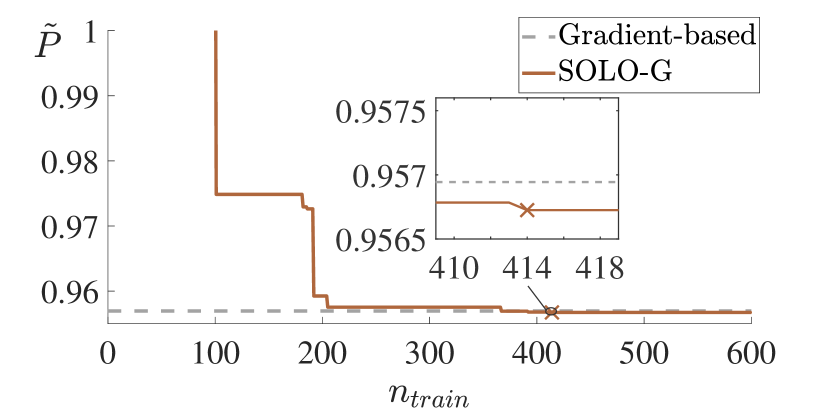 \SetHorizontalCoffin\labelcoffin
c\SetVerticalPole\imagecoffinleft3pt+\CoffinWidth\labelcoffin/2\SetVerticalPole\imagecoffinright\Width-3pt-\CoffinWidth\labelcoffin/2\SetHorizontalPole\imagecoffinup\Height-3pt-\CoffinHeight\labelcoffin/2\SetHorizontalPole\imagecoffindown3pt+\CoffinHeight\labelcoffin/2\JoinCoffins\imagecoffin[left,up]\labelcoffin[vc,hc]\TypesetCoffin\imagecoffin
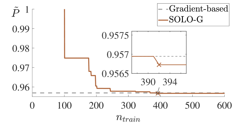 \SetHorizontalCoffin\labelcoffin
d\SetVerticalPole\imagecoffinleft3pt+\CoffinWidth\labelcoffin/2\SetVerticalPole\imagecoffinright\Width-3pt-\CoffinWidth\labelcoffin/2\SetHorizontalPole\imagecoffinup\Height-3pt-\CoffinHeight\labelcoffin/2\SetHorizontalPole\imagecoffindown3pt+\CoffinHeight\labelcoffin/2\JoinCoffins\imagecoffin[left,up]\labelcoffin[vc,hc]\TypesetCoffin\imagecoffin
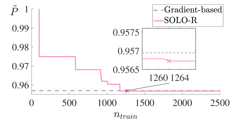 \SetHorizontalCoffin\labelcoffin
a\SetVerticalPole\imagecoffinleft3pt+\CoffinWidth\labelcoffin/2\SetVerticalPole\imagecoffinright\Width-3pt-\CoffinWidth\labelcoffin/2\SetHorizontalPole\imagecoffinup\Height-3pt-\CoffinHeight\labelcoffin/2\SetHorizontalPole\imagecoffindown3pt+\CoffinHeight\labelcoffin/2\JoinCoffins\imagecoffin[left,up]\labelcoffin[vc,hc]\TypesetCoffin\imagecoffin
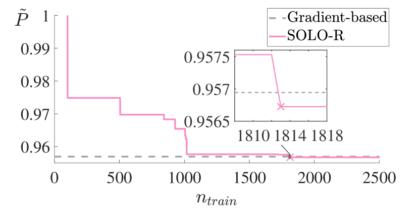 \SetHorizontalCoffin\labelcoffin
b\SetVerticalPole\imagecoffinleft3pt+\CoffinWidth\labelcoffin/2\SetVerticalPole\imagecoffinright\Width-3pt-\CoffinWidth\labelcoffin/2\SetHorizontalPole\imagecoffinup\Height-3pt-\CoffinHeight\labelcoffin/2\SetHorizontalPole\imagecoffindown3pt+\CoffinHeight\labelcoffin/2\JoinCoffins\imagecoffin[left,up]\labelcoffin[vc,hc]\TypesetCoffin\imagecoffin
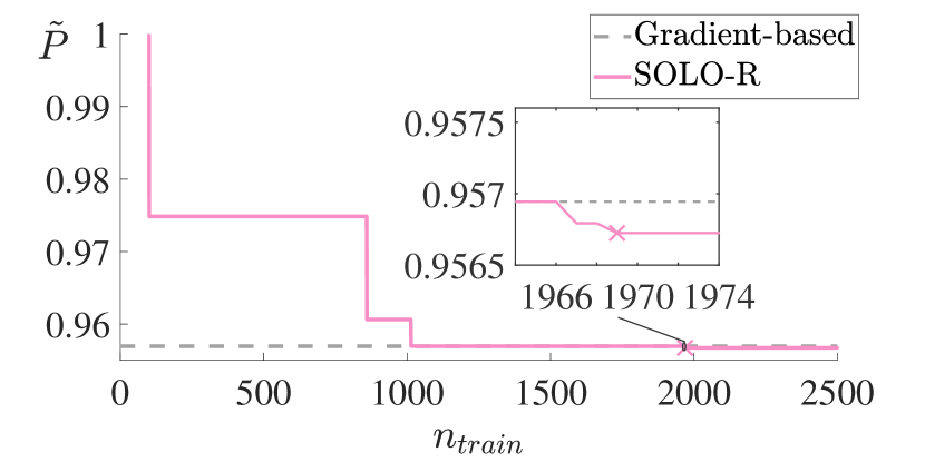 \SetHorizontalCoffin\labelcoffin
c\SetVerticalPole\imagecoffinleft3pt+\CoffinWidth\labelcoffin/2\SetVerticalPole\imagecoffinright\Width-3pt-\CoffinWidth\labelcoffin/2\SetHorizontalPole\imagecoffinup\Height-3pt-\CoffinHeight\labelcoffin/2\SetHorizontalPole\imagecoffindown3pt+\CoffinHeight\labelcoffin/2\JoinCoffins\imagecoffin[left,up]\labelcoffin[vc,hc]\TypesetCoffin\imagecoffin
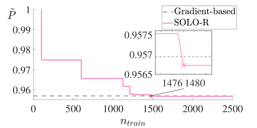 \SetHorizontalCoffin\labelcoffin
d\SetVerticalPole\imagecoffinleft3pt+\CoffinWidth\labelcoffin/2\SetVerticalPole\imagecoffinright\Width-3pt-\CoffinWidth\labelcoffin/2\SetHorizontalPole\imagecoffinup\Height-3pt-\CoffinHeight\labelcoffin/2\SetHorizontalPole\imagecoffindown3pt+\CoffinHeight\labelcoffin/2\JoinCoffins\imagecoffin[left,up]\labelcoffin[vc,hc]\TypesetCoffin\imagecoffin
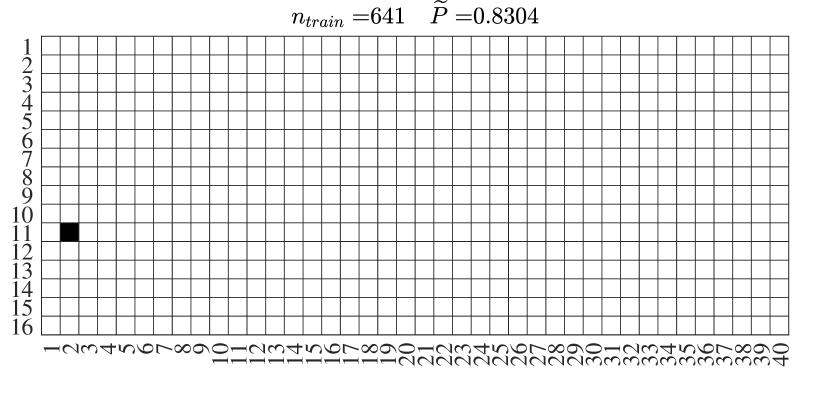 \SetHorizontalCoffin\labelcoffin
a\SetVerticalPole\imagecoffinleft3pt+\CoffinWidth\labelcoffin/2\SetVerticalPole\imagecoffinright\Width-3pt-\CoffinWidth\labelcoffin/2\SetHorizontalPole\imagecoffinup\Height-3pt-\CoffinHeight\labelcoffin/2\SetHorizontalPole\imagecoffindown3pt+\CoffinHeight\labelcoffin/2\JoinCoffins\imagecoffin[left,up]\labelcoffin[vc,hc]\TypesetCoffin\imagecoffin
b\SetVerticalPole\imagecoffinleft3pt+\CoffinWidth\labelcoffin/2\SetVerticalPole\imagecoffinright\Width-3pt-\CoffinWidth\labelcoffin/2\SetHorizontalPole\imagecoffinup\Height-3pt-\CoffinHeight\labelcoffin/2\SetHorizontalPole\imagecoffindown3pt+\CoffinHeight\labelcoffin/2\JoinCoffins\imagecoffin[left,up]\labelcoffin[vc,hc]\TypesetCoffin\imagecoffin
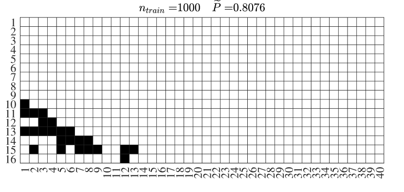 \SetHorizontalCoffin\labelcoffin
c\SetVerticalPole\imagecoffinleft3pt+\CoffinWidth\labelcoffin/2\SetVerticalPole\imagecoffinright\Width-3pt-\CoffinWidth\labelcoffin/2\SetHorizontalPole\imagecoffinup\Height-3pt-\CoffinHeight\labelcoffin/2\SetHorizontalPole\imagecoffindown3pt+\CoffinHeight\labelcoffin/2\JoinCoffins\imagecoffin[left,up]\labelcoffin[vc,hc]\TypesetCoffin\imagecoffin
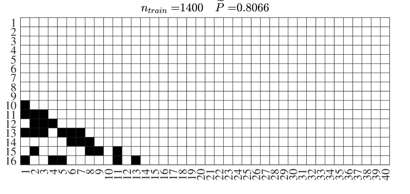 \SetHorizontalCoffin\labelcoffin
d\SetVerticalPole\imagecoffinleft3pt+\CoffinWidth\labelcoffin/2\SetVerticalPole\imagecoffinright\Width-3pt-\CoffinWidth\labelcoffin/2\SetHorizontalPole\imagecoffinup\Height-3pt-\CoffinHeight\labelcoffin/2\SetHorizontalPole\imagecoffindown3pt+\CoffinHeight\labelcoffin/2\JoinCoffins\imagecoffin[left,up]\labelcoffin[vc,hc]\TypesetCoffin\imagecoffin
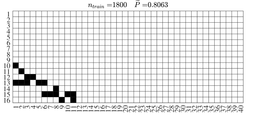 \SetHorizontalCoffin\labelcoffin
e\SetVerticalPole\imagecoffinleft3pt+\CoffinWidth\labelcoffin/2\SetVerticalPole\imagecoffinright\Width-3pt-\CoffinWidth\labelcoffin/2\SetHorizontalPole\imagecoffinup\Height-3pt-\CoffinHeight\labelcoffin/2\SetHorizontalPole\imagecoffindown3pt+\CoffinHeight\labelcoffin/2\JoinCoffins\imagecoffin[left,up]\labelcoffin[vc,hc]\TypesetCoffin\imagecoffin
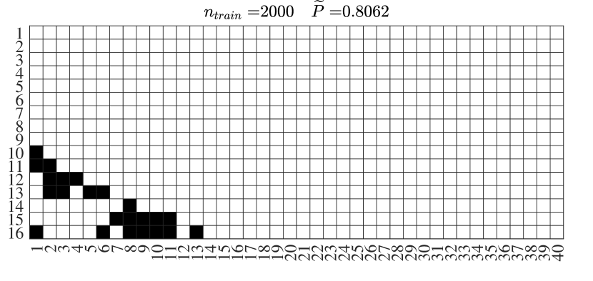 \SetHorizontalCoffin\labelcoffin
f\SetVerticalPole\imagecoffinleft3pt+\CoffinWidth\labelcoffin/2\SetVerticalPole\imagecoffinright\Width-3pt-\CoffinWidth\labelcoffin/2\SetHorizontalPole\imagecoffinup\Height-3pt-\CoffinHeight\labelcoffin/2\SetHorizontalPole\imagecoffindown3pt+\CoffinHeight\labelcoffin/2\JoinCoffins\imagecoffin[left,up]\labelcoffin[vc,hc]\TypesetCoffin\imagecoffin
 \SetHorizontalCoffin\labelcoffin
a\SetVerticalPole\imagecoffinleft3pt+\CoffinWidth\labelcoffin/2\SetVerticalPole\imagecoffinright\Width-3pt-\CoffinWidth\labelcoffin/2\SetHorizontalPole\imagecoffinup\Height-3pt-\CoffinHeight\labelcoffin/2\SetHorizontalPole\imagecoffindown3pt+\CoffinHeight\labelcoffin/2\JoinCoffins\imagecoffin[left,up]\labelcoffin[vc,hc]\TypesetCoffin\imagecoffin
 \SetHorizontalCoffin\labelcoffin
b\SetVerticalPole\imagecoffinleft3pt+\CoffinWidth\labelcoffin/2\SetVerticalPole\imagecoffinright\Width-3pt-\CoffinWidth\labelcoffin/2\SetHorizontalPole\imagecoffinup\Height-3pt-\CoffinHeight\labelcoffin/2\SetHorizontalPole\imagecoffindown3pt+\CoffinHeight\labelcoffin/2\JoinCoffins\imagecoffin[left,up]\labelcoffin[vc,hc]\TypesetCoffin\imagecoffin
 \SetHorizontalCoffin\labelcoffin
c\SetVerticalPole\imagecoffinleft3pt+\CoffinWidth\labelcoffin/2\SetVerticalPole\imagecoffinright\Width-3pt-\CoffinWidth\labelcoffin/2\SetHorizontalPole\imagecoffinup\Height-3pt-\CoffinHeight\labelcoffin/2\SetHorizontalPole\imagecoffindown3pt+\CoffinHeight\labelcoffin/2\JoinCoffins\imagecoffin[left,up]\labelcoffin[vc,hc]\TypesetCoffin\imagecoffin
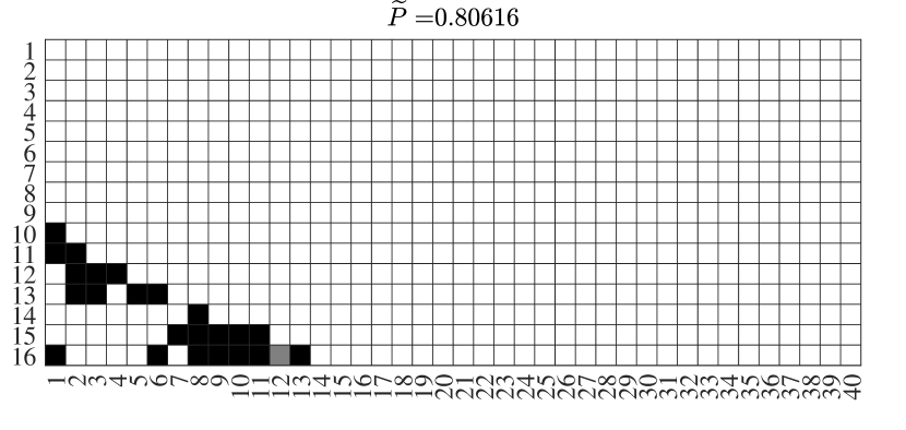 \SetHorizontalCoffin\labelcoffin
d\SetVerticalPole\imagecoffinleft3pt+\CoffinWidth\labelcoffin/2\SetVerticalPole\imagecoffinright\Width-3pt-\CoffinWidth\labelcoffin/2\SetHorizontalPole\imagecoffinup\Height-3pt-\CoffinHeight\labelcoffin/2\SetHorizontalPole\imagecoffindown3pt+\CoffinHeight\labelcoffin/2\JoinCoffins\imagecoffin[left,up]\labelcoffin[vc,hc]\TypesetCoffin\imagecoffin
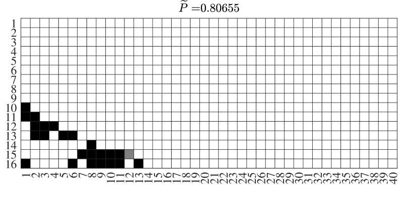 \SetHorizontalCoffin\labelcoffin
e\SetVerticalPole\imagecoffinleft3pt+\CoffinWidth\labelcoffin/2\SetVerticalPole\imagecoffinright\Width-3pt-\CoffinWidth\labelcoffin/2\SetHorizontalPole\imagecoffinup\Height-3pt-\CoffinHeight\labelcoffin/2\SetHorizontalPole\imagecoffindown3pt+\CoffinHeight\labelcoffin/2\JoinCoffins\imagecoffin[left,up]\labelcoffin[vc,hc]\TypesetCoffin\imagecoffin
 \SetHorizontalCoffin\labelcoffin
f\SetVerticalPole\imagecoffinleft3pt+\CoffinWidth\labelcoffin/2\SetVerticalPole\imagecoffinright\Width-3pt-\CoffinWidth\labelcoffin/2\SetHorizontalPole\imagecoffinup\Height-3pt-\CoffinHeight\labelcoffin/2\SetHorizontalPole\imagecoffindown3pt+\CoffinHeight\labelcoffin/2\JoinCoffins\imagecoffin[left,up]\labelcoffin[vc,hc]\TypesetCoffin\imagecoffin
 \SetHorizontalCoffin\labelcoffin
g\SetVerticalPole\imagecoffinleft3pt+\CoffinWidth\labelcoffin/2\SetVerticalPole\imagecoffinright\Width-3pt-\CoffinWidth\labelcoffin/2\SetHorizontalPole\imagecoffinup\Height-3pt-\CoffinHeight\labelcoffin/2\SetHorizontalPole\imagecoffindown3pt+\CoffinHeight\labelcoffin/2\JoinCoffins\imagecoffin[left,up]\labelcoffin[vc,hc]\TypesetCoffin\imagecoffin
 \SetHorizontalCoffin\labelcoffin
h\SetVerticalPole\imagecoffinleft3pt+\CoffinWidth\labelcoffin/2\SetVerticalPole\imagecoffinright\Width-3pt-\CoffinWidth\labelcoffin/2\SetHorizontalPole\imagecoffinup\Height-3pt-\CoffinHeight\labelcoffin/2\SetHorizontalPole\imagecoffindown3pt+\CoffinHeight\labelcoffin/2\JoinCoffins\imagecoffin[left,up]\labelcoffin[vc,hc]\TypesetCoffin\imagecoffin
 \SetHorizontalCoffin\labelcoffin
i\SetVerticalPole\imagecoffinleft3pt+\CoffinWidth\labelcoffin/2\SetVerticalPole\imagecoffinright\Width-3pt-\CoffinWidth\labelcoffin/2\SetHorizontalPole\imagecoffinup\Height-3pt-\CoffinHeight\labelcoffin/2\SetHorizontalPole\imagecoffindown3pt+\CoffinHeight\labelcoffin/2\JoinCoffins\imagecoffin[left,up]\labelcoffin[vc,hc]\TypesetCoffin\imagecoffin
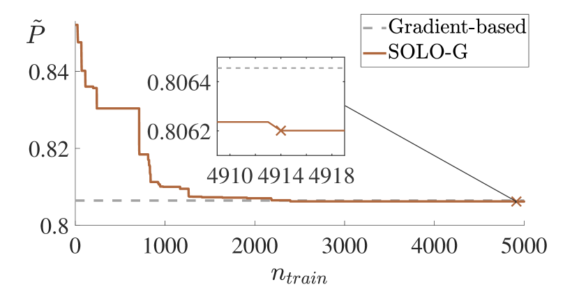 \SetHorizontalCoffin\labelcoffin
a\SetVerticalPole\imagecoffinleft3pt+\CoffinWidth\labelcoffin/2\SetVerticalPole\imagecoffinright\Width-3pt-\CoffinWidth\labelcoffin/2\SetHorizontalPole\imagecoffinup\Height-3pt-\CoffinHeight\labelcoffin/2\SetHorizontalPole\imagecoffindown3pt+\CoffinHeight\labelcoffin/2\JoinCoffins\imagecoffin[left,up]\labelcoffin[vc,hc]\TypesetCoffin\imagecoffin
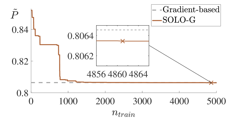 \SetHorizontalCoffin\labelcoffin
b\SetVerticalPole\imagecoffinleft3pt+\CoffinWidth\labelcoffin/2\SetVerticalPole\imagecoffinright\Width-3pt-\CoffinWidth\labelcoffin/2\SetHorizontalPole\imagecoffinup\Height-3pt-\CoffinHeight\labelcoffin/2\SetHorizontalPole\imagecoffindown3pt+\CoffinHeight\labelcoffin/2\JoinCoffins\imagecoffin[left,up]\labelcoffin[vc,hc]\TypesetCoffin\imagecoffin
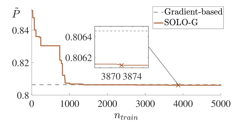 \SetHorizontalCoffin\labelcoffin
c\SetVerticalPole\imagecoffinleft3pt+\CoffinWidth\labelcoffin/2\SetVerticalPole\imagecoffinright\Width-3pt-\CoffinWidth\labelcoffin/2\SetHorizontalPole\imagecoffinup\Height-3pt-\CoffinHeight\labelcoffin/2\SetHorizontalPole\imagecoffindown3pt+\CoffinHeight\labelcoffin/2\JoinCoffins\imagecoffin[left,up]\labelcoffin[vc,hc]\TypesetCoffin\imagecoffin
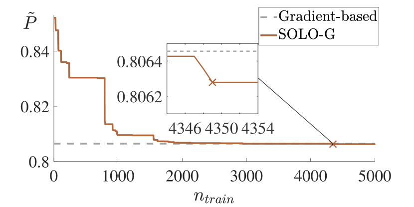 \SetHorizontalCoffin\labelcoffin
d\SetVerticalPole\imagecoffinleft3pt+\CoffinWidth\labelcoffin/2\SetVerticalPole\imagecoffinright\Width-3pt-\CoffinWidth\labelcoffin/2\SetHorizontalPole\imagecoffinup\Height-3pt-\CoffinHeight\labelcoffin/2\SetHorizontalPole\imagecoffindown3pt+\CoffinHeight\labelcoffin/2\JoinCoffins\imagecoffin[left,up]\labelcoffin[vc,hc]\TypesetCoffin\imagecoffin
a
b

c
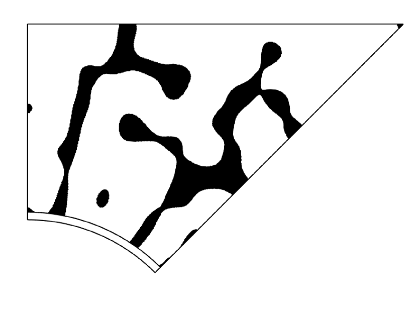
d
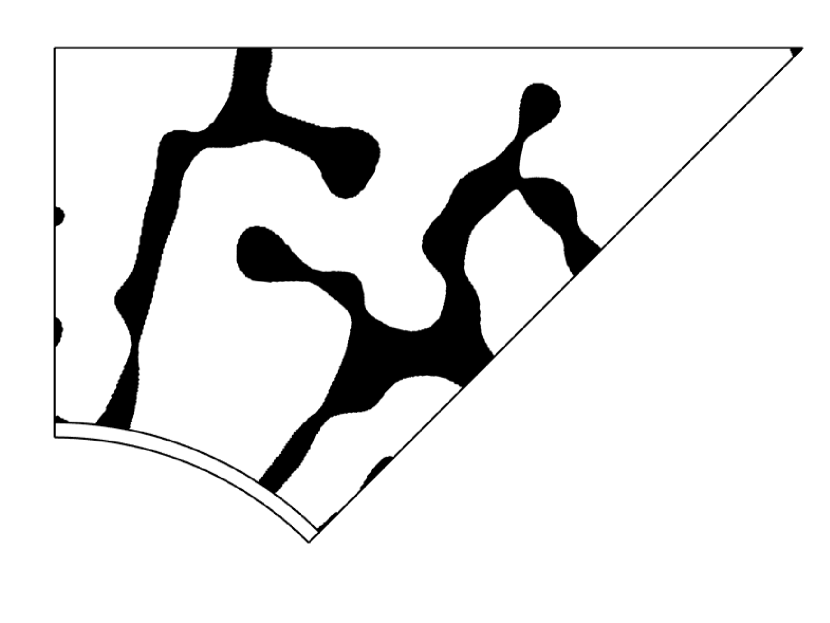
e

f

2 Theory on convergence
In the main text, we presented a simplified version of convergence (Eq. (3)). In this section, we give a detailed description of our theoretical result. We first present the main result (Theorem 1). Then, we introduce some preliminary definitions and knowledge used in the proof. In the end, we approach the proof.
2.1 Formulation and theorem
The unknown object function is denoted as , where .We denote the domain of as . We suppose the global minimizer .
We consider the total iteration number to be . At iteration , the DNN is denoted as and we denote the empirical minimizer of this DNN function to be , i.e.
| (S1) |
Besides, we denote our DNN as a -layer neural network which is formulated as follows:
where (number of input dimensions), , and is the ReLU69 activation function for . We further denote and the function class of such neural networks as .
At time step , given the empirical optimal point , the additional training points is generated through the following process:
Here denotes random noise for perturbation. Hence through the iterating process, the sampled points are random variables. At time step , we denote all the realizations of random training data points set as .
Now before we proceed, we need to impose some mild assumptions on the problem.
Assumption 1.
We suppose that
-
1)
the spectral norm of the matrices in DNNs are uniformly bounded, i.e., there exists s.t. .
-
2)
the target function is bounded, i.e., there exists s.t. .
1) of Assumption 1 is a commonly studied assumption in existing generalization theory literature on deep neural networks 70, 71, 72. 2) of Assumption 1 assumes is bounded, which is standard and intuitive since has a physical meaning.
Assumption 2.
We assume that for any iteration , are i.i.d. (independent and identically distributed) perturbation noise. The generated training data are independent of if .
The assumption of the i.i.d. properties of noise in Assumption 2 is common in optimization literature 73, 74, 75, 76. The difference is that in traditional optimization literature noise refers to the difference between the true gradient and the stochastic gradient while the noise here denotes perturbations to generate new samples in each iteration. Note that our Assumption 2 only needs the i.i.d. property of noise, which is weaker than the standard assumptions for stochastic gradient methods which require unbiased property and bounded variance 74, 75, 76. Since our fitting DNN s are continuously changing throughout iterations and the empirical minimizers are also alternating, it is reasonable for us to assume that the different groups of generated data samples are independent for the ease of theoretical analysis in the sequel.
We denote the distribution of samples as , with which we can introduce the following definition.
Definition 1.
For a measurable function , we denote
| (S2) |
where denotes expectation.
Assumption 3.
For any and ,
where is a monotonically decreasing function w.r.t. iteration number .
Assumption 3 basically describes that the Chebyshev distance of our DNN at time and is bounded by a constant number (w.r.t. ) times the average true loss of till time . This assumption is reasonable in that the the average true loss can be seen as a variant of Euclidean distance between our DNN at time and .
Eventually we arrive at our main result.
Theorem 1.
where .
2.2 Preliminaries
Before showing the complete proof, we introduce some definitions and lemmas.
Lemma 1 (McDiarmid’s Inequality77).
Let be a set of independent random variables and assume that there exist such that satisfies the following conditions:
for all and any points . Here s are the realizations of s. Let denote , then, for all , the following inequality hold:
| (S3) | |||
| (S4) |
where denotes probability and denotes expectation.
Definition 2 (Covering Number78).
Let be a normed space, and . Vector set is an -covering of if ) where denotes the ball with center and radius , equivalently, such that . The covering number is defined as :
Definition 3 (Rademacher Complexity & Empirical Rademacher Complexity79, 78).
Given a sample and a set of real-valued function , the Empirical Rademacher Complexity is defined as
where sup denotes supremum and the expectation is over the Rademacher random variables , which are i.i.d. (independent and identically distributed) with . The Rademacher Complexity is defined as
which is the expectation of the Empirical Rademacher Complexity over sample .
Lemma 2 (Dudley’s Entropy Integral Bound72).
Given a sample , let be a real-valued function class taking values in for some constant , and assume that zero function . Then we have
where inf denotes infimum.
Lemma 3.
(Covering number bound using volume ratio72) Let be the set of matrices with bounded spectral norm and be given. The covering number is upper bounded by
2.3 Proof
This subsection presents the complete proof of Theorem 1. We first give a proof sketch.
Proof sketch
We provide a sketch of proof of Theorem 1 for readers’ convenience. First by the property of our algorithm and telescoping, we can get
| (S5) |
(S5) means that when function can fit the target function very well, the universal convergence can be guaranteed. By Assumption 3, we can rewrite (S5) as
| (S6) |
Then we can employ the standard argument of Rademacher Complexity to bound the RHS of (S6) and then obtain
| (S7) |
where function class and can be viewed as the supreme of the training error ( by our assumption, can be arbitrarily small). Then utilizing Lemma 2, we have
| (S8) |
where denotes the covering number. Then through investigating the Lipschitz property of w.r.t to its parameter set, employing the argument of volume ratio (Lemma 3) and setting as , we can bound the covering number by
| (S9) |
Finally combining (S6), (2.3), (S8) and (S9), we get the desired universal convergence result.
Before showing the full proof, we introduce an auxiliary lemma here.
Lemma 4.
Under Assumptions 2, we have
-
1)
the whole generated data points are mutually independent.
-
2)
for any , are i.i.d..
Now we can approach the proof of Theorem 1.
Proof.
We first bound term by telescoping:
| (S10) |
Here (i) comes from Eq. (S1), (ii) uses the fact that for any real number and , we have . (iii) arises from Assumption 3.
For notational simplicity we further denote
| (S11) |
where corresponds to the empirical MSE loss when training our neural network.
Suppose and are two samples which are different only in the -th point, namely and , we have
then by Mcdiarmid’s Inequality (Eq.(S3) in Lemma 1), we get
| (S12) |
Given any , by setting the right hand side of (2.3) to be , we have with probability at least ,
| (S13) |
Notice that
| (S14) |
Here the second equality in Eq. (2.3) is because:
where (i) results from 1) of Lemma 4 and (ii) comes from 2) of Lemma 4.
Further we have
| (S15) |
where are Rademacher variables (Definition 3), which are uniformly distributed independent random variables taking values in . Here (i) and (iii) hold due to the sub-additivity of the supremum function (considering the convexity of supremum function, by Jensen’s Inequality, we have for any function , holds). (ii) combines the definition of Rademacher variable and the fact that the expectation is taken over both and .
For notational simplity, given any function , we define the non-negative loss function and its function class .
Then combining (2.3) and (2.3) we obtain
| (S16) |
where is the Rademacher Complexity (Definition 3) of .
Now, we define the Empirical Rademacher Complexity of as
Again, suppose and are two samples which are different only in the -th point, namely and , we have
then by Mcdiarmid’s Inequality (Eq.(S4) in Lemma 1), we get
| (S17) |
Given any , by setting the right handside of Eq.(2.3) to be , we have with probability at least ,
| (S18) |
Now combining (S13), (S16) and (S18), we get with probability at least ,
| (S19) |
here we use the fact that (S13) and (S18) hold with probability respectively and that .
It is straightforward that , then Dudley’s Entropy (Lemma 2) gives us
| (S20) |
where denotes the covering number. We pick , and combine (2.3), (S19) and (2.3) to get
| (S21) |
Next we need to compute the covering number . To derive a tight covering number we investigate the Lispchitz continuity of with respect to the weight matrices . Consider two neural networks and with different sets of weight matrices, we first notice that
Next we get the bound based on weight matrices. Specifically, given two different sets of matrices and , we have
Note that we have
where (i) comes from the definition of the ReLU activation, (ii) comes from and recursion, and (iii) comes from the boundedness of . Accordingly, we have
| (S22) |
where (i) comes from the fact that , and (ii) comes from the recursion. Considering the fact that each corresponds to its parameter set , we can then derive the covering number of by the Cartesian product of the matrix covering of :
| (S23) |
Here (i) utilizes the fact that if , matrix set
is a covering of set , then by (S22) we have function set
is an covering of . (ii) comes from the fact that for any matrix we have , and (iii) employs Lemma 3. Plugging (S23) into (2.3), we get
| (S24) |
Since we consider the empirical MSE training loss to be less than , i.e.,
| (S25) |
so by plugging (S25) into (2.3), we get the desired result. ∎