Diffusive interaction of multiple surface nanobubbles and nanodroplets: shrinkage, growth, and coarsening

Abstract

Surface nanobubbles are nanoscopic spherical-cap shaped gaseous domains on immersed substrates which are stable, even for days. After the stability of a single surface nanobubble has been theoretically explained, i.e. contact line pinning and gas oversaturation are required to stabilize them against diffusive dissolution [Lohse and Zhang, Phys. Rev. E 91, 031003 (R) (2015)], here we focus on the collective diffusive interaction of multiple nanobubbles. For that purpose we develop a finite difference scheme for the diffusion equation with the appropriate boundary conditions and with the immersed boundary method used to represent the growing or shrinking bubbles. After validation of the scheme against the exact results of Epstein and Plesset for a bulk bubble [J. Chem. Phys. 18, 1505 (1950)] and of Lohse and Zhang for a surface bubble, the framework of these simulations is used to describe the coarsening process of competitively growing nanobubbles. The coarsening process for such diffusively interacting nanobubbles slows down with advancing time and thus increasing bubble distance. The present results for surface nanobubbles are also applicable for immersed surface nanodroplets, for which better controlled experimental results of the coarsening process exist.

I Introduction

Surface nanobubbles lohse2015rmp – nanoscopic gaseous domains on immersed surfaces – were first speculated to exist about 20 years ago parker1994 and later found in atomic force microscopy (AFM) images ishida2000 ; tyrrell2001 ; lou2000 . While their long-time existence (often days) was first considered as puzzling craig2011softmatter due to the supposedly large internal Laplace pressure, which should squeeze them out, it is now theoretically understood that they are stable thanks to a stable balance between the Laplace pressure inside the nanobubble and the gas overpressure from outside, which is enabled by pinning of the contact line zhang2013langmuir ; liu2013jcp ; liu2014jcp2 ; lohse2015 ; lohse2015rmp . The equilibrium angle $\theta_{e}$ (see figure 1 for a sketch of the surface nanobubble and the used notation) is determined by the gas oversaturation $\zeta=c_{\infty}/c_{s}-1$, where $c_{\infty}$ is the concentration far away and $c_{s}$ the solubility, and the contact diameter $L$ by lohse2015

$$\sin\theta_{e}=\zeta{L\over L_{c}},$$ (1)

where $L_{c}=4\sigma/P_{0}=2.84\mu m$ for air in water under ambient pressure $P_{0}=1$ bar and with its surface tension $\sigma=0.072N/m$. Note that we have assumed a spherical-cap shape, which is well-justified theoretically and experimentally. The experimental confirmation of equation (1) through AFM experiments is difficult for various reasons lohse2015rmp , but it was confirmed in molecular dynamics (MD) simulations maheshwari2016b .

In this paper we will first add further numerical confirmation of the theory of Ref. (lohse2015, ) by directly solving the diffusion equation around a surface nanobubble, together with the appropriate boundary conditions, namely $c_{\infty}$ far away from the bubble, no gas flux through the substrate, and a gas concentration given by Henry’s law at the bubble-liquid interface, finding perfect agreement for the equilibrium contact angle $\theta_{e}$ (Eq. (1)) (section III). Before, in section II, we will introduce the employed numerical method, namely a finite difference scheme coupled to an immersed boundary method fad00 ; peskin2002 ; mittal2005 .

Note that Eq. (1) implies that the Young-Laplace relation, which determines the contact angle on a macroscopic scale due to the mutual interfacial tensions, is irrelevant on the microscopic scale of the nanobubbles. This is in agreement with various experimental observations (see e.g. song2011 ; lohse2015rmp ) that the microscopic contact angle is constant and independent of the substrate and thus different from the macroscopic contact angle. According to Eq. (1), the crossover from macroscopic to microscopic bubbles occurs at the length scale $L_{c}/\zeta$, below which the bubbles are small enough so that their Laplace pressure is large enough to counteract the gas influx by oversaturation.

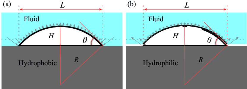
Figure 1: Sketch and notation of a surface droplet. L is the contact diameter, $\theta$ the contact angle, H the maximum height of the droplet, and R the radius of curvature.

The main focus of the present paper will however be on multiple surface bubbles which are diffusively interacting lohse2015 ; peng2016mega ; zhang2013langmuir ; german2014 . In general, no analytical solution is possible for this case. An exception is the case of two diffusively interacting surface bubbles far away from each other, i.e., with a distance $d$ much larger than their surface contact diameter $L$. For that case Dollet and Lohse dollet2016 succeeded to analytically show that the pinning of the surface bubbles not only stabilizes each bubble against dissolution or growth, but that it also stabilizes the pair of surface bubbles against Ostwald ripening voorhees1985 , i.e., the shrinkage of a bubble with smaller radius of curvature (corresponding to large Laplace pressure) to the benefit of a neighboring bubble with larger radius of curvature. Here we will numerically show that this stabilization of a pair of surface bubbles through pinning holds in general, i.e., is not limited to bubbles far away from each other. We will also show that the lack of pinning leads to Ostwald ripening (section III).

In section V we will extend the calculation to many surface nanobubbles in a row, studying their coarsening process. The coarsening of nanobubbles in principle can happen via Ostwald ripening or via coalescence. In Ref. peng2015acsnano the analogous coarsening process of nanodroplets growing in an oversaturated solution was experimentally studied. There the nanodroplets also effectively sit in a row, namely at the rim of a spherical lense, and our assumption of periodic boundary conditions for the bubbles is justified. In that reference peng2015acsnano it was speculated that the coarsening mainly happens via Ostwald ripening. Here within our model we will show under what conditions this indeed can be the case. We will moreover study the dynamics of the coarsening process and show that it slows down with advancing time and thus increasing distance between the bubbles, similar to other coarsening processes meer2004 .

As mentioned above, our numerical scheme can not only be applied to diffusively interacting nanobubbles in a liquid, but equally well to diffusively interacting droplets in a liquid (see e.g. our own work on this subject, Refs. peng2015acsnano ; zhang2015pnas ; tan2016 ) or in a gas, e.g., as they emerge in dew formation beysens1986 ; family1989 ; rose2002 ; leach2006 ; stricker2015 .

The paper ends with conclusions and an outlook (section VI).

II Method: Finite differences coupled to the immersed boundary method

We start by considering the diffusion equation

$$\frac{\partial c}{\partial t}=D\nabla^{2}c+s,$$ (2)

where $c$ is the concentration field, $D$ the diffusion coefficient. In the immersed boundary boundary methods peskin2002 ; mittal2005 , the Eulerian source term $s$ is used to mimic the effects of the boundaries of bubbles or droplets on the concentration.

The boundaries of bubbles or droplets are discretized into a series of Lagrangian points. The Eulerian and Lagrangian sources are related to each other through a regularized delta function

$$s(\mathbf{x})=\int S(\mathbf{X}_{l})\delta(\mathbf{x}-\mathbf{X}_{l})\mathrm{d}s,$$ (3)

where $\mathbf{x}$ and $\mathbf{X}_{l}$ are the position vectors of the Eulerian and Lagrangian points; $S$ the Lagrangian source term; $\delta$ the delta function, respectively.

To enforce the prescribed concentration fields on the boundary, we define the Lagrangian concentration field. Using the regularized delta function again, this relation can be expressed as follows

$$\int c(\mathbf{x})\delta(\mathbf{x}-\mathbf{X}_{l})d\mathbf{x}=C_{\Gamma}(\mathbf{X}_{l}),$$ (4)

where $C_{\Gamma}$ is the Lagrangian concentration field which is prescribed, known beforehand, on the boundary.

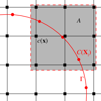
Figure 2: Schematic sketch to illustrate the immersed boundary method: The diffusion equation is solved on the Eulerian Cartesian grid points $\bf x$. The boundary $\Gamma$ is discretized into a set of Lagrangian points $\bf X$. The transfers of the concentration between the Eulerian and the Lagrangian grid ($c\to C$) and the source term between the Lagrangian and Eulerian gird ($S\to s$) are through the discrete regularized delta function $\delta_{h}$, which covers the area $A$.

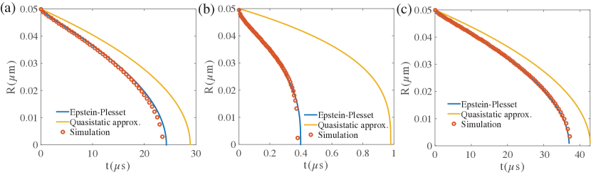
Figure 3: Time evolution of the bubble radius $R(t)$ for nitrogen gas bubble for three cases with $c_{\infty}=0$ and the same initial bubble radius 50 nm: (a) The bubble surface concentration and the gas density stay constant during the diffusion. (b) The gas density stays the same, however the surface concentration is given by Henry’s law, where $C_{\Gamma}(R,t)=c_{s}(1+2\sigma/R)$. (c) The gas density varies according to the ideal gas law and the surface concentration according to Henry’s law as in (b). In the simulations here, the domain size is $0.5\mu$m$\times$$0.5\mu$m$\times$$0.5\mu$m. The resolution is of the computational domain is $201\times 201\times 201$. Our numerical solutions agree very well with the exact Epstein-Plesset epstein1950 results. However, our results deviate from that of a quasistatic approximation $\partial_{t}c=0$.

In the discretized form, the diffusion equation for the $k$th step is solved through the following procedures. First, an intermediate “guessed” concentration field $\mathrm{bar}c$ is calculated from the Eulerian source term of the last step $s^{k-1}$, with

$$\mathrm{bar}c=c^{k-1}+\Delta t(D\nabla^{2}c^{k-1}+s^{k-1}).$$ (5)

Here, the diffusion term $\nabla^{2}c$ is discretized by a second-order explicit scheme.

Next, we interpolate the intermediate concentration field from Eulerian ($\mathrm{bar}c$) to Lagrangian ($\mathrm{bar}C$) grid points through the discrete delta function $\delta_{h}$, i. e.

$$\mathrm{bar}C({\bf X}_{l})=\sum_{{\bf x}\in A}\mathrm{bar}c({\bf x})\delta_{h}({\bf x}-{\bf X}_{l})h^{3}.$$ (6)

Apparently $\mathrm{bar}C$ does not satisfy the boundary condition $C_{\Gamma}$. In order to achieve $C_{\Gamma}$, from Eqn. 5 the Lagrangian source term $S^{k}$ for the current time step is derived as

$$S^{k}=S^{k-1}+\frac{C_{\Gamma}-\mathrm{bar}C}{\Delta t}.$$ (7)

The next step is to spread the Lagrangian source term $S^{k}$ to the Eulerian counterpart $s^{k}$ through the discrete delta function $\delta_{h}$ again, expressed as

$$s^{k}({\bf x})=\sum_{m=1}^{N_{L}}S^{k}({\bf x})\delta_{h}({\bf x}-{\bf X}_{l})\Delta V_{l}.$$ (8)

Finally, the concentration field with the Eulerian source term $s^{k}$ at $k$th step is solved from

$$\left(1-D\Delta t\frac{\nabla^{2}}{2}\right)c^{k}=c^{k-1}+\Delta t\left(D\frac{\nabla^{2}c^{k-1}}{2}+s^{k}\right).$$ (9)

Here the Crank-Nicolson scheme is adopted to ensure the stability of the code.

This ends one time step, after which the next time step is treated in the same way.

The regularized delta function used in the present study is defined as

$$\delta_{h}(\textbf{x}-\textbf{X})=\frac{1}{h^{3}}\phi(\frac{x-X}{h})\phi(\frac{y-y}{h})\phi(\frac{z-Z}{h}),$$ (10)

where $\phi$ in the present implementation is based on the four-point version of Peskin peskin2002 .

$$\phi(r)=\left\{{\begin{array}[]{*{20}c}{{\textstyle{1\over 8}}\left({3-2\left|r\right|+\sqrt{1+4\left|r\right|-4r^{2}}}\right),\mathop{}\nolimits\left|r\right|\leq 1,}\\ {{\textstyle{1\over 8}}\left({5-2\left|r\right|-\sqrt{-7+12\left|r\right|-4r^{2}}}\right),\mathop{}\nolimits 1\leq\left|r\right|\leq 2,}\\ {0,\mathop{}\nolimits\mathop{}\nolimits\mathop{}\nolimits\mathop{}\nolimits\mathop{}\nolimits\mathop{}\nolimits\mathop{}\nolimits\mathop{}\nolimits\mathop{}\nolimits\mathop{}\nolimits\mathop{}\nolimits 2\leq\left|r\right|,}\\ \end{array}}\right.$$ (11)

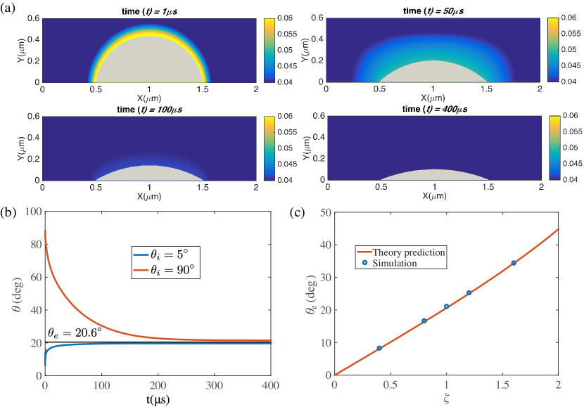
Figure 4: (a) Snapshots of the diffusive dynamics of a pinned surface nanobubbles growing towards its equilibrium state. The color code represents the gas concentration field. Here $L=1$ $\mu$m and $\zeta=1$. (b) Time evolution $\theta(t)$ of the contact angle growing or shrinking towards its equilibrium value $\theta_{e}$ given by Eq. (1). Two cases with different initial contact angles $\theta_{i}$ are shown. As above, $L=1$ $\mu$m and $\zeta=1$. (c) Equilibrium contact angle $\theta_{e}$ for various gas concentrations $\zeta$. The straight line is the prediction Eq. (1), giving perfect agreement. Again, $L=1$ $\mu$m. In the simulations here, the domain size is $6\mu$m$\times$$3\mu$m$\times$$6\mu$m. The resolution is of the computational domain is $301\times 151\times 301$. The corresponding videos are shown as supplementary material.

III Validation of the scheme for a single bulk bubble and a single surface bubble

We will now validate the scheme introduced in the previous section. We will assume two test cases: a spherical bubble in the bulk, whose growth or shrinkage behavior is analytically known since Epstein and Plesset epstein1950 (section III.1), and a surface nanobubble, which in the pinned case has a stable equilibrium contact angle given by Eq. (1), and in the unpinned case either shrinks and then fully dissolves or grows and then finally detaches (section III.2). All the simulations that are shown below are performed with nitrogen bubble, for which the material parameters are $D=2\times 10^{-9}$ m²/s, $\rho_{g}=1.165$ kg/m³, and $c_{s}=0.017$ kg/m³.

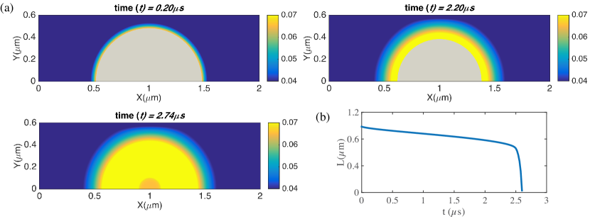
Figure 5: Time evolution for the contact diameter $L(t)$ for an unpinned surface nanobubble with pre-described constant contact angle o$\theta=90^{\circ}$ and gas oversaturation $\zeta=1$. The bubble dissolves within 3 microseconds. In the simulations here, the domain size is $6\mu$m$\times$$3\mu$m$\times$$6\mu$m. The resolution is of the computational domain is $301\times 151\times 301$. The corresponding videos are shown as supplementary material.

III.1 The Epstein-Plesset bubble

In still liquid in an infinite domain, the mass loss or gain of a spherical bubble of radius $R$ is given by the concentration gradient $\left(\frac{\partial c}{\partial r}\right)_{R}$ at its surface and the diffusion constant $D$,

$$\frac{dm}{dt}=\frac{d(4/3\rho\pi R^{3})}{dt}=4\pi R^{2}D\left(\frac{\partial c}{\partial r}\right)_{R}.$$ (12)

Here $\rho$ the density of gas in the bubble. Epstein-Plesset epstein1950 succeeded to solve the diffusion equation together with Eq. (12) and the boundary condition far away from the bubble, $c(r\to\infty,t)=c_{\infty}$, to obtain an ordinary differential equation (ODE) for the bubble radius $R(t)$,

$$\frac{dR}{dt}=-\frac{(C_{\Gamma}-c_{\infty})D}{\rho}\left[\frac{1}{R}+\frac{1}{(\pi Dt)^{1/2}}\right].$$ (13)

Here the prescribed $C_{\Gamma}$ is calculated from Henry’s law, taking the effects of surface tension into account, i.e., $C_{\Gamma}(R,t)=c_{s}(1+2\sigma/R)$, where $c_{s}$ is the saturation concentration. Note that for small bubbles the Laplace pressure leads to an enhanced density, obtained from the ideal gas law, and this effect of the surface tension must also be taken into account. Equation (13) can be solved analytically to obtain $R(t)$ epstein1950 . Obviously, also in the simulations the bubble is assumed to keep its spherical shape during the diffusion process and equation (12) is used to update the bubble radius and the Lagrangian coordinate $\bf{X}$ during the simulation.

Our numerical results of the relation between the bubble radius and time based on the scheme developed in the previous section are shown in figure 3 and compared with the analytical results (or the results from Eq. (13)). Three cases are considered. In figure 3(a), the bubble surface concentration and gas density are kept constant, in figure 3(b), the density of the gas is kept constant and we use the Henry’s law to calculate $C_{\Gamma}$, and in figure 3(c), we vary the density of the bubble according to the ideal gas law and again the Henry’s law is used to calculate $C_{\Gamma}$. For all the cases, our simulations show excellent agreements with the predictions from Eq. (13).

We now come to dissolving or growing surface bubbles and droplets (“sessile droplets”) cazabat2010 ; lohse2015rmp . For this axisymmetric case, Popov popov2005 could exactly solve the quasi-static case $\partial_{t}c\approx 0$, i.e., the diffusion equation reduces to a Laplace question. For evaporating droplets as in the case of Popov, this in general is a very good approximation. Later the Popov model was also applied to surface nanobubbles lohse2015 . Then the gas concentration at the interface is again given by Henry’s law which for surface bubbles takes the form $C_{\Gamma}(R,t)=c_{s}[1+4\sigma\sin\theta/(P_{0}L)]$.

To check how important the time dependence of the concentration field is, we apply Popov’s model for a dissolving bubble with a fixed contact angle of 90^∘, written as

$$\frac{dR}{dt}=-\frac{(C_{\Gamma}-c_{\infty})D}{\rho}\frac{1}{R}.$$ (14)

One can see that the only difference between Eq. (13) and Eq. (14) is that in Eq. (14) the time dependent term in the right hand side of Eq. (13) is eliminated. It is observed from figure 3 that when Henry’s law is used while the bubble density is kept constant, the quasi-static assumption of Popov’s model leads to an overestimation of the bubble lifetime. Therefore in the following, for appropriately simulating the diffusive dynamics of the bubbles, we do not use the quasi-static approximation, but employ the full diffusion equation with Henry’s law for the bubble surface concentration and the ideal gas law for the bubble density.

III.2 Stability of surface nanobubble & confirmation of the theory of Lohse & Zhang lohse2015

For nano-bubbles with pinned contact line, an ODE for the diffusive contact angle dynamics was derived in Ref. lohse2015 , namely

$$\frac{d\theta}{dt}=-\frac{4D}{L^{2}}\frac{c_{s}}{\rho}(1+\cos\theta)^{2}f(\theta)\left[\frac{L_{c}}{L}\sin\theta-\zeta\right],$$ (15)

with

$$f(\theta)=\frac{\sin\theta}{1+\cos\theta}+4\int_{0}^{\infty}\frac{1+\cosh 2\theta\tau}{\sinh 2\pi\tau}\tanh[(\pi-\theta)\tau]d\tau.$$ (16)

A stable nanobubble can therefore be formed with the condition of Eq. (1) where the bubble contact angle $\theta$ is a constant and stable.

Figure 4(a) shows snapshots for the bubble evolution in the pinned case with $L=1\mu$m and $\zeta=1$, for which according to Eq. (1) there should be a stable equilibrium lohse2015 , for fixed gas oversaturation $\zeta>0$. Indeed, the stable equilibrium angle $\theta_{e}=20.6^{\circ}$ is reached in the simulations. Figure 4(b) shows the time evolution of the contact angle for two initial contact angles $\theta_{i}=90^{\circ}$ and $\theta_{i}=5^{\circ}$. In both cases the contact angles saturate to the predicted $\theta_{e}=20.6^{\circ}$ when advancing time long enough. Further, we vary the oversaturation rate $\zeta$ from 0.4 to 1.6, in which the equilibrium contact angle $\theta$ would change, as shown in figure 4(c). Again our results are in perfect agreement with the prediction (Eq. (1)).

In comparison, when a bubble is unpinned, even if with gas oversaturation, the bubble can not be stable because of the Laplace pressure, In figure 5, we show the time evolution of a bubble in a constant contact mode with fixed contact angle $\theta=90^{o}$. The oversaturation $\zeta=1$ but still the bubble dissolves very quickly.

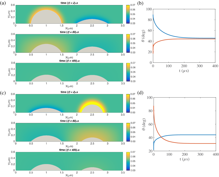
Figure 6: (a), (c): Snapshots of the time evolution of two pinned neighbouring bubbles and the surrounding gas concentration field. The oversaturation is $\zeta=2$. For (a), the contact diameters are $L_{1}=L_{2}=1$ $\mu$m. The initial contact angle for the left bubble is $90^{\circ}$ and for the right bubble is $15^{\circ}$. For (c), the contact diameters are $L_{1}=1$ $\mu$m and $L_{2}=0.7$ $\mu$m. The initial contact angle for the left bubble is $15^{\circ}$ and for the right bubble is $90^{\circ}$. The pinning stabilizes the two bubbles against Ostwald ripening and the contact angles of both bubbles converge to $\theta_{e}$, as given by Eq. (1). (b), (d): Contact angles of the two bubbles as function of time for cases (a) and (c). In (d) (case (c), and in (b) (case (a)) of course anyhow), the resulting radii of curvature $L/\cos\theta_{e}$ are identical. In the simulations here, the domain size is $6\mu$m$\times$$3\mu$m$\times$$6\mu$m. The resolution is of the computational domain is $301\times 151\times 301$. The corresponding videos are shown as supplementary material.

We take the opportunity here to discuss the assumptions that lead to Eq. (15). Henry’s law is used when deriving Eq. (15), however the gas density is assumed constant and the process is assumed quasi-steady. Let’s first focus on the quasi-steady assumption. The typical diffusion time scale is $t_{d}=R^{2}/D$, while the evaporation/dissolution time scale $t_{e}=t_{d}\rho/(c_{s}-c_{\infty})$. For a water droplet evaporation, $t_{e}/t_{d}$ is of the order of $10^{5}$, thus Eq. (15) is a rather good approximation gelderblom2011 without considering the time dependent term of the diffusion equation. However, for a gas bubble, $t_{e}/t_{d}$ is of the order of $10^{2}$, thus the quasi-steady condition can not be valid anymore, as also shown in figure 3(b). Also the gas density might vary because of the Laplace pressure. However, it is easy to see from Eq. (15) and Eq. (3) that these considerations are only relevant for the time scale of the evolution towards the equilibrium contact angle $\theta_{e}$, not for the value of $\theta_{e}$ itself.

IV Ostwald ripening process of two bubbles: unpinned vs pinned case

We now move to the case of two bubbles, for which the general argument for nanobubble stability is not available anymore. One exception is the case where two bubbles are far away from each other. For this case Dollet and Lohse dollet2016 theoretically show that pinning also suppresses the Ostwald ripening process between neighbouring surface nanobubbles. But this case is not given in most experiments, in which the nanobubbles sit very close to each other and nonetheless can remain stable for very long time zhang2013langmuir . In this paper we will now show with numerical simulations that this stabilization of a pair of surface bubbles through pinning is indeed not limited to bubbles far away from each other but also holds for bubbles that are close.

Figure 6 shows two cases, the first one for two surface bubbles with same fixed contact diameter $L_{1}=L_{2}=1$ $\mu$m and the second one with different contact diameters $L_{1}=1$ $\mu$m, $L_{2}=0.7$ $\mu$m. In both cases we set the oversaturation to $\zeta=2$ and have pinned contact lines. It can be seen that with pinning and gas oversaturation, indeed the two bubbles case are eventually stable, even if the distance between them are very close. Specifically, for the case with same contact diameter, both have the stable equilibrium contact angle $\theta_{e}=40.7^{\circ}$ given by equation (1). For the case with different contact diameters, one bubble has the stable equilibrium contact angle $\theta_{e}=40.7^{\circ}$ and the other one $\theta_{e}=29.6^{\circ}$, however, the radii of curvature $L/\cos\theta_{e}$ for the two bubbles are the same, as it should be according to the theory of Lohse and Zhang lohse2015 .

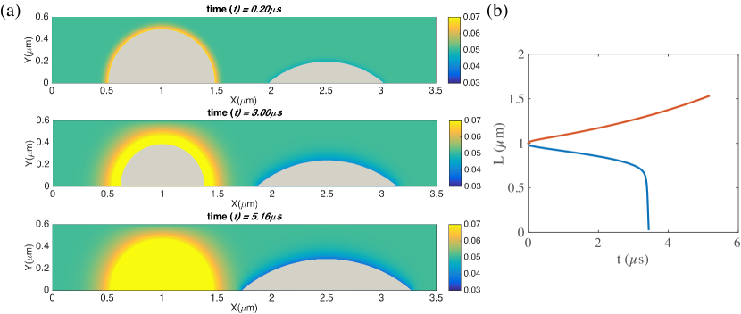
Figure 7: (a) Snapshots of the time evolution of two unpinned neighbouring bubbles and the surrounding gas concentration field. The parameters are the same as in the case of figure 6(a). In the absence of pinning the pair of bubbles undergoes Ostwald ripening, i.e., one bubble grows and the other ones dissolves. (b) Contact diameters of the two bubbles as function of time. The red curve shows the contact diameter of the growing right bubble, and the blue one that of the shrinking left bubble, which is fully dissolved in the end. In the simulations here, the domain size is $6\mu$m$\times$$3\mu$m$\times$$6\mu$m. The resolution is of the computational domain is $301\times 151\times 301$. The corresponding videos are shown as supplementary material.

For the bubbles with unpinned contact line, Ostwald ripening indeed diffusively destabilizes the two neighboring bubble. In figure 7 we show two bubbles with the same condition as in figure 6(a)(b), but now unpinned and with constant contact angles. It can be seen that the two bubbles diffusively interact with each other, leading to Ostwald ripening: Therefore one bubbles dissolves and the other one grows.

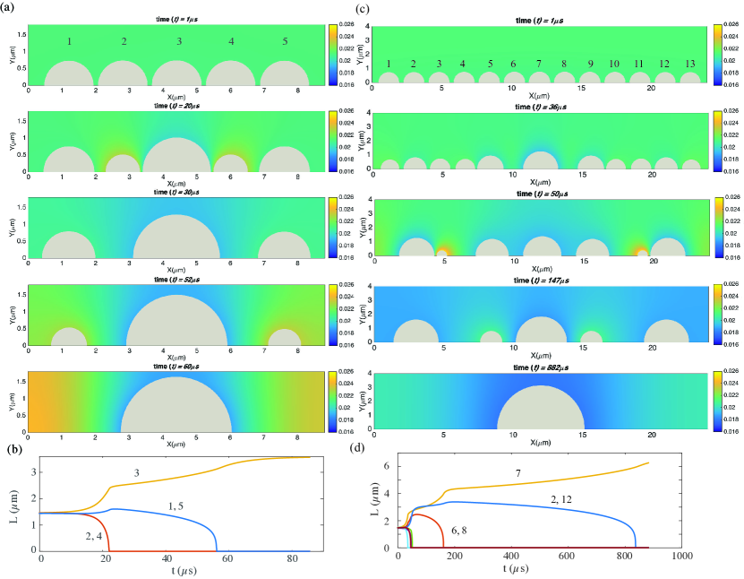
Figure 8: (a) Coarsening processes for five neighboring bubbles in a row. The oversaturation is $\zeta=1$. The five bubbles have slightly different initial contact diameters, i.e. bubble 1 and bubble 5 have 1.44 $\mu$m, bubble 2 and bubble 4 have 1.45 $\mu$m, and bubble 3 has 1.46 $\mu$m. The bubbles are in the constant contact angle mode. (b) The time evolution of the contact diameters for the 5 bubbles. (c) and (d): The same as (a) and (b), but now for thirteen initial bubbles. Bubble contact diameters are from 1.44 $\mu$m to 1.5 $\mu$m, with an increase of 0.01 $\mu$m for each from bubble 1 to bubble 7. Then from bubble 7 to bubble 13, the contact diameter decreases 0.01 $\mu$m for each. Here we can use the two-dimensional axis-symmetric simulations because the contact angle is $90^{\circ}$. For (a), the domain size is $8.8\mu$m$\times$$3\mu$m. The resolution is is $881\times 301$. For (c), the domain size is $24\mu$m$\times$$4\mu$m. The resolution is is $2401\times 401$. The corresponding videos are shown as supplementary material.

V Diffusive coarsening process for an one-dimensional array of bubbles

Finally, we look at the coarsening process for an one-dimensional array of bubbles. In figure 8(a), we show an array of 5 bubbles. The bubbles all have a constant contact angle of $90^{\circ}$. Initially, bubble 1 and bubble 5 have contact diameters of 1.44 $\mu$m, bubble 2 and bubble 4 have contact diameters of 1.45 $\mu$m, and bubble 3 has a contact diameter of 1.46 $\mu$m. Because of the Henry’s law, smaller bubble will have a higher surface concentration while bigger one lower. Thus a concentration gradient between different bubbles is formed and the coarsening process starts. Interestingly, it is not bubble 1 and 5, which have the lowest surface concentration that are eaten by other bubbles, but bubble 2 and 4, which are in between. We see after the disappearance of bubbles 2 and 4, all other three bubbles become bigger, however with time advancing, the even bigger bubble 3 finally eats all the other bubbles and the coarsening process ends. Similar effects can be found for more bubbles, in figure 8(c), we show an array of 13 bubbles. In this case, bubble contact diameters are from 1.44 $\mu$m to 1.5 $\mu$m, with an increase of 0.01 $\mu$m for each from bubble 1 to bubble 7. Then from bubble 7 to bubble 13, the contact diameter decreases 0.01 $\mu$m for each. Analogous to the coarsening process of shaken compartimentalized granular matter of Ref. meer2004 , here for nanobubbles we find that with time passing by and thus the distance between the bubbles growing, the coarsening process also slows down, as shown in figures 8(b,d).

VI Conclusions and outlook

Simulations of finite difference combined with the immersed boundary methods were performed to study the stability and instability of nanobubbles. Four difference configurations were considered, a bulk bubble, a surface bubble, two close surface bubbles, and an array of surface bubbles. For bulk bubbles, the simulated time evolution of the bubble radius shows excellent agreements with Epstein & Plesset’s analytical results epstein1950 , validating our scheme and code. For single surface nanobubbles, our simulations confirm that pinning and oversaturation can indeed stabilize the surface nanobubble, and the equilibrium contact angle perfectly agrees with the analytical result Eq. (1) of Lohse and Zhang lohse2015 . Thus a consistent picture between our prior theoretical calculations and the present numerical simulations has emerged. For two neighbouring nanobubbles, we find that pinning and oversaturation can stabilize the nanobubble pair against Ostwald ripening, even when the bubbles are very close to each other. Finally, we show the coarsening process for a row of nanobubbles. The coarsening slows down with advancing time and increasing nanobubble distance, similar to the coarsening process as seen in shaken compartimentalized granular matter meer2004 .

We note that though here we give the results only for surface nanobubbles, corresponding results should also hold for surface nanodroplets. We also note that for the parameters of this study here, the dominant coarsening process is Ostwald ripening, i.e., mass exchange by diffusion, but for other parameters (e.g. larger oversaturation) the dominant process can also be bubble coalescence. To map out the parameter space when Ostwald ripening will be dominant and when bubble coalescence will be the subject of future work. Correspondingly, in future work we also want to extend this study from surface bubbles or surface droplets in a row to those in a two-dimensional array as experimentally done in e.g. Refs. bao2016 ; german2014 or to randomly distributed surface bubbles or droplets as in Ref. zhang2015pnas . Future work can also address how heterogeneities on the gas-water interfaces through e.g. local surfactant accumulation can affect the overall dynamics of the bubble ensemble.

Finally, we caution the reader: Our results are based on continuum theory and hydrodynamic equations. However, at very short length scales the continuum approximation will break down. In very recent molecular dynamics (MD) simulations, Maheshwari et al. maheswari2018 have revealed that in certain cases (very strong attraction between the dissolved gas molecules and the surface) surface nanobubbles very close to each other can communicate through a “new channel”, namely diffusion of gas from one surface bubble to the other along the surface, and not through the bulk. If this is the case, some sort of ripening process of neighboring surface bubbles may be possible in spite of hydrodynamic stability against Ostwald ripening.

Conflicts of interest

There are no conflicts to declare.

References

- (1) D. Lohse and X. Zhang, Surface nanobubble and surface nanodroplets, Rev. Mod. Phys. 87, 981 (2015).
- (2) J. L. Parker, P. M. Claesson, and P. Attard, Bubbles, cavities and the long-ranged attraction between hydrophobic surfaces, J. Phys. Chem. 98, 8468 (1994).
- (3) N. Ishida, T. Inoue, M. Miyahara, and K. Higashitani, Nano bubbles on a hydrophobic surface in water observed by tapping-mode atomic force microscopy, Langmuir 16, 6377 (2000).
- (4) J. W. G. Tyrrell and P. Attard, Images of nanobubbles on hydrophobic surfaces and their interactions, Phys. Rev. Lett. 87, 176104 (2001).
- (5) S.-T. Lou, Z.-Q. Ouyang, Y. Zhang, X.-J. Li, J. Hu, M.-Q. Li, and F.-J. Yang, Nanobubbles on solid surface imaged by atomic force microscopy, J. Vac. Sci. Technol. B 18, 2573 (2000).
- (6) V. S. J. Craig, Very small bubbles at surfaces – the nanobubble puzzle, Soft Matter 7, 40 (2011).
- (7) X. Zhang, D. Y. C. Chan, D. Wang, and N. Maeda, Stability of Interfacial Nanobubbles, Langmuir 29, 1017 (2013).
- (8) Y. Liu and X. Zhang, Nanobubble stability induced by contact line pinning, J. Chem. Phys. 138, 014706 (2013).
- (9) Y. Liu and X. Zhang, A unified mechanism for the stability of surface nanobubbles: Contact line pinning and supersaturation, J. Chem. Phys. 141, 134702 (2014).
- (10) D. Lohse and X. Zhang, Pinning and gas oversaturation imply stable single surface nanobubble, Phys. Rev. E 91, 031003(R) (2015).
- (11) S. Maheshwari, M. van der Hoef, X. Zhang, and D. Lohse, Stability of Surface Nanobubbles: A Molecular Dynamics Study, Langmuir 32, 11116 (2016).
- (12) E. A. Fadlun, R. Verzicco, P. Orlandi, and J. Mohd-Yusof, Combined immersed boundary/finite-difference methods for three-dimensional complex flow simulations, J. Comp. Phys. 161, 35 (2000).
- (13) C. S. Peskin, The immersed boundary method, Acta Numer. 11, 479 (2002).
- (14) R. Mittal and G. Iaccarino, Immersed boundary methods, Annu. Rev. Fluid Mech. 37, 239 (2005).
- (15) B. Song, W. Walczyk, and H. Schönherr, Contact Angles of Surface Nanobubbles on Mixed Self-Assembled Monolayers with Systematically Varied Macroscopic Wettability by Atomic Force Microscopy, Langmuir 27, 8223 (2011).
- (16) S. Peng, T. L. Mega, and X. Zhang, Collective Effects in Microbubble Growth by Solvent Exchange, Langmuir 32, 11265 (2016).
- (17) S. R. German, X. Wu, H. An, V. S. J. Craig, T. L. Mega, and X. Zhang, Interfacial Nanobubbles Are Leaky: Permeability of the Gas/Water Interface, ACS Nano 8, 6193 (2014).
- (18) B. Dollet and D. Lohse, Pinning Stabilizes Neighboring Surface Nanobubbles against Ostwald Ripening, Langmuir 32, 11335 (2016).
- (19) P. W. Voorhees, The theory of Ostwald ripening, J. Stat. Phys. 38, 231 (1985).
- (20) S. Peng, D. Lohse, and X. Zhang, Spontaneous Pattern Formation of Surface Nanodroplets from Competitive Growth, ACS Nano 9, 11916 (2015).
- (21) D. van der Meer, K. van der Weele, and D. Lohse, Coarsening dynamics in a vibrofluidized compartmentalized granular gas, Journal of Statistical Mechanics: Theory and Experiment 2004, P04004 (2004).
- (22) X. Zhang, Z. Lu, H. Tan, L. Bao, Y. He, C. Sun, and D. Lohse, Formation of surface nanodroplets under controlled flow conditions, Proc. Nat. Acad. Sci. 112, 9253 (2015).
- (23) H. Tan, C. Diddens, P. Lv, J. G. M. Kuerten, X. Zhang, and D. Lohse, Evaporation-triggered microdroplet nucleation and the four life phases of an evaporating Ouzo drop, Proc. Nat. Acad. Sci. 113, 8642 (2016).
- (24) D. Beysens and C. M. Knobler, Growth of Breath figures, Phys. Rev. Lett. 57, 1433 (1986).
- (25) F. Family and P. Meakin, Kinetics of droplet growth processes: Simulations, theory, and experiments, Phys. Rev. A 40, 3836 (1989).
- (26) J. W. Rose, Dropwise condensation theory and experiment: a review, Proc. Inst. Mech. Eng. A 216, 115 (2002).
- (27) R. N. Leach, F. Stevens, S. C. Langford, and J. T. Dickinson, Dropwise condensation: Experiments and simulations of nucleation and growth of water drops in a cooling system, Langmuir 22, 8864 (2006).
- (28) L. Stricker and J. Vollmer, Impact of microphysics on the growth of one-dimensional breath figures, Phys. Rev. E 92, 042406 (2015).
- (29) P. S. Epstein and M. S. Plesset, On the stability of gas bubbles in liquid-gas solutions, J. Chem. Phys. 18, 1505 (1950).
- (30) A. M. Cazabat and G. Guéna, Evaporation of macroscopic sessile droplets, Soft Matter 6, 2591 (2010).
- (31) Y. O. Popov, Evaporative deposition patterns: Spatial dimensions of the deposit, Phys. Rev. E 71, 036313 (2005).
- (32) H. Gelderblom, A. G. Marin, H. Nair, A. van Houselt, L. Lefferts, J. H. Snoeijer, and D. Lohse, How water droplets evaporate on a superhydrophobic substrate, Phys. Rev. E 83, 026306 (2011).
- (33) L. Bao, Z. Werbiuk, D. Lohse, and Z. Zhang, Controlling the growth modes of femtoliter sessile droplets nucleating on chemically patterned surfaces, J. Phys. Chem. Lett. 7, 1055 (2016).
- (34) S. Maheshwari, M. van der Hoef, J. Rodriguez-Rodriguez, and D. Lohse, Leakiness of pinned neighboring surface nanobubbles induced by strong gas-surface interaction, ACS Nano 12, 2603 (2018).