Metric preheating and radiative decay in single-field inflation

Abstract

At the end of inflation, the inflaton oscillates at the bottom of its potential and these oscillations trigger a parametric instability for scalar fluctuations with wavelength $\lambda$ comprised in the instability band $(3Hm)^{-1/2}<\lambda<H^{-1}$, where $H$ is the Hubble parameter and $m$ the curvature of the potential at its minimum. This “metric preheating” instability, which proceeds in the narrow resonance regime, leads to various interesting phenomena such as early structure formation, production of gravitational waves and formation of primordial black holes. In this work we study its fate in the presence of interactions with additional degrees of freedom, in the form of perturbative decay of the inflaton into a perfect fluid. Indeed, in order to ensure a complete transition from inflation to the radiation-dominated era, metric preheating must be considered together with perturbative reheating. We find that the decay of the inflaton does not alter the instability structure until the fluid dominates the universe content. As an application, we discuss the impact of the inflaton decay on the production of primordial black holes from the instability. We stress the difference between scalar field and perfect fluid fluctuations and explain why usual results concerning the formation of primordial black holes from perfect fluid inhomogeneities cannot be used, clarifying some recent statements made in the literature.

1 Introduction

Cosmic inflation [1, 2, 3, 4, 5] is presently the most promising paradigm to describe the physical conditions that prevailed in the very early universe. It consists of two stages. First, there is a phase of accelerated expansion. In the simplest models, it is driven by a scalar field, the inflaton, slowly rolling down its potential, and the background spacetime almost exponentially expands. Second, there is the reheating epoch [6, 7, 8, 9, 10, 11, 12] (see Refs. [13, 14] for reviews) during which the inflaton field oscillates around the minimum of its potential and decays into other degrees of freedom it couples to. Then, after thermalisation of these decay products, the radiation-dominated era of the hot big-bang phase starts.

One of the main successes of the inflationary scenario is that it provides a convincing mechanism for the origin of the structures in our universe [15, 16]. According to the inflationary paradigm, they stem from quantum fluctuations born on sub-Hubble scales and subsequently amplified by gravitational instability and stretched to super-Hubble distances by cosmic expansion. During this process, which occurs in the slow-roll phase, cosmological perturbations acquire an almost scale-invariant power spectrum, which is known to provide an excellent fit to the astrophysical data at our disposal [17, 18].

In the simplest models where inflation is driven by a single scalar field with canonical kinetic term, on large scales, the curvature perturbation is conserved [15, 16], which implies that the details of the reheating process do not affect the inflationary predictions or, in other words, that “metric preheating” is inefficient on those scales. Since these models are well compatible with the data [19, 20, 21, 22], the stage of reheating is usually not considered as playing an important role in the evolution of cosmological perturbations [23]. For the scales observed in the Cosmic Microwave Background (CMB), the only effect of reheating is through the amount of expansion that proceeds during this epoch, which relates physical scales as we observe today to the time during inflation when they emerge. This thus determines the part of the inflationary potential that we probe with the CMB. In practice, there is a single combination [24] of the reheating temperature and of the mean equation-of-state parameter, that sets the location of the observational window along the inflationary potential. Given the restrictions on the shape of the potential now available [20, 25], this can be used to constrain the kinematics of reheating [26, 27, 28, 29]. In multiple-field scenarios, on the contrary, large-scale curvature perturbations can be strongly distorted by the reheating process [30, 31, 32, 33, 34], which means that metric preheating can be important and, thus, can have more impact on CMB observations.

The situation is very different for scales smaller than those observed in the CMB, more precisely for scales crossing back in the Hubble radius during reheating (or never crossing out the Hubble radius during inflation). In particular, it was shown in LABEL:Jedamzik:2010dq (see also LABEL:Easther:2010mr) that the density contrast of the scalar field fluctuations can grow on small scales during preheating, due to a parametric instability sourced by the oscillations of the inflaton at the bottom of its potential. This mechanism demonstrates that metric preheating can be important even in single-field inflation, although not on large scales. It can give rise to different interesting phenomena such as early structure formation [35], gravitational waves production [37] and even Primordial Black Holes (PBHs) [38, 39] formation [40] (PBHs formation from scalar fields was considered in LABEL:Khlopov:1985jw, in the case of two-fields models in LABEL:Bassett:2000ha and in the case of single-field tachyonic preheating in LABEL:Suyama:2006sr).

These phenomena can lead to radical shifts in the standard picture of how reheating proceeds. Indeed, in LABEL:Martin:2019nuw, it was shown that the production of light PBHs from metric preheating is so efficient that they can quickly come to dominate the universe content, such that reheating no longer occurs because of the inflaton decay, as previously described, but rather through PBHs Hawking evaporation. This conclusion, however, was reached by neglecting the decay products of the inflaton throughout the instability phase, and by simply assuming that they would terminate the instability abruptly at the time when they dominate the energy budget (if PBHs have not come to dominate the universe before then). However, as will be made explicit below, the instability of metric preheating proceeds in the narrow resonance regime. One may therefore be concerned that it requires a delicate balance in the dynamics of the system, and that even a small amount of produced radiation could be enough to distort or jeopardise the instability mechanism. The goal of this paper is therefore to investigate how the presence of inflaton decay products (modelled as a perfect fluid), produced by perturbative reheating, affects the metric preheating instability.

The paper is organised as follows. In Sec. 2, we briefly review metric preheating, which leads to the growth of the inflaton density contrast at small scales. Then, in Sec. 3, we study whether a small amount of radiation, originating from the inflaton decay, can modify this growth. For this purpose, we introduce a covariant coupling model between the inflaton scalar field and a perfect fluid, leading to equations of motion at the background (see Sec. 3.1) and perturbative (see Sec. 3.2) levels that feature no substantial change in the instability structure until the fluid dominates. In Sec. 3.3, we discuss the application of the previous results to the production of PBHs during reheating, which, we stress, cannot be described as originating from perfect fluid inhomogeneities, contrary to what is sometimes argued. Finally, in Sec. 4, we briefly summarise our main results and present our conclusions.

2 Preheating in single-field inflation

In this work, we consider single scalar field models of inflation, with a canonical kinetic term. In these models, a homogeneous inflaton field $\phi(t)$ drives the expansion of a flat Friedmann-Lemaître-Robertson-Walker (FLRW) space-time, described by the metric $\mathrm{d}s^{2}=-\mathrm{d}t^{2}+a^{2}(t)\mathrm{d}{\bm{x}}^{2}$, where $a(t)$ is the FLRW scale factor. The corresponding equations of motion are the Friedmann and Klein-Gordon equations, namely

$$H^{2}=\frac{1}{3M_{\scriptscriptstyle{\mathrm{Pl}}}^{2}}\left[\frac{\dot{\phi}^{2}}{2}+V(\phi)\right],\quad\ddot{\phi}+3H\dot{\phi}+V_{\phi}\left(\phi\right)=0\,,$$ (2.1)

where $H=\dot{a}/a$ is the Hubble parameter, $V_{\phi}$ the derivative of the potential with respect to $\phi$, $M_{\scriptscriptstyle{\mathrm{Pl}}}$ the reduced Planck mass and a dot denotes a derivative with respect to cosmic time $t$. The inflaton field potential $V(\phi)$ must be such that the potential energy dominates over the kinetic energy of the inflaton, and inflation ($\ddot{a}>0$) ends when they become comparable, that is to say when the first slow-roll parameter $\epsilon_{1}\equiv-\dot{H}/H^{2}$ reaches one. This usually happens in the vicinity of a local minimum of the potential. There, most potentials can be approximated by a quadratic function, $V(\phi)\sim m^{2}\phi^{2}/2$, where $m$ is the curvature of the potential at its minimum. In fact, this expression can be seen as a leading-order Taylor expansion of the potential around its minimum, and it is not valid only for potentials having an exactly vanishing mass at their minimum, for which the leading term is of higher order. When the inflaton reaches this region of the potential, it oscillates according to $\phi(t)\propto a^{-3/2}\sin\left(mt\right)$, the expansion becomes, on average, decelerated, and similar to that of a matter-dominated universe [9], i.e. $\langle\rho\rangle\propto a^{-3}$ (where $\langle\cdot\rangle$ denotes averaging over one oscillation).

2.1 Perturbative reheating

These considerations however ignore the possible coupling of the inflaton with other degrees of freedom. In order to incorporate it, several descriptions are possible. A simple way, which corresponds to “perturbative reheating”, consists in introducing a term “$\Gamma\dot{\phi}$” (where $\Gamma$ is a decay rate) in the Klein-Gordon equation to account for the decay of the inflaton into a perfect fluid (typically radiation) [6, 7, 8, 12]. In this case, the friction term becomes $(3H+\Gamma/2)\dot{\phi}$. Initially, $H\gg\Gamma$ and the effect of the inflaton decay is negligible, until $H$ crosses down $\Gamma$, at a time around which most of the decay of the inflaton occurs. In the next section, we explain how to introduce $\Gamma$ covariantly, thus allowing us to perform a consistent treatment both at the background and perturbative levels. Microscopically, if one considers for instance that $\phi$ is coupled to another scalar field $\chi$ through the interaction Lagrangian ${\cal L}_{\mathrm{int}}=-2g^{2}\sigma\phi\chi^{2}$, where $g$ is a dimensionless coupling constant and $\sigma$ a new mass scale, the corresponding decay rate can be calculated within perturbation theory and one finds $\Gamma=g^{4}\sigma^{2}/(4\pi m)$ [12]. If this process occurs at sufficiently high energy, the mass of the $\chi$-particles are small compared to the Hubble parameter at decay and, effectively, the inflaton field decays into relativistic matter or radiation.

2.2 Non-perturbative preheating

The above perturbative description is however not sufficient since non-perturbative effects can also play an important role [10, 11, 12]. This can be simply illustrated if one considers the case where the interaction Lagrangian reads ${\cal L}_{\mathrm{int}}=-g^{2}\phi^{2}\chi^{2}/2$. If one denotes the monotonously decreasing amplitude of the inflaton oscillations as $\phi_{0}(t)$, such that $\phi\simeq\phi_{0}(t)\sin(mt)$, then the equation of motion of the Fourier transform $\chi_{\bm{k}}$ of the field $\chi$ reads

$$\ddot{\chi}_{\bm{k}}+3H\dot{\chi}_{\bm{k}}+\left[\frac{k^{2}}{a^{2}(t)}+m_{\chi}^{2}+g^{2}\phi_{0}^{2}(t)\sin^{2}(mt)\right]\chi_{\bm{k}}=0\,,$$ (2.2)

where $m_{\chi}$ is the mass of $\chi$ and ${\bm{k}}$ the wavenumber of the mode under consideration. Writing $X_{\bm{k}}=a^{3/2}\chi_{\bm{k}}$ and using the variable $z\equiv mt$, the above equation can also be written under the following form

$$\frac{\mathrm{d}^{2}X_{\bm{k}}}{\mathrm{d}z^{2}}+\left[A_{\bm{k}}-2q\cos\left(2z\right)\right]X_{\bm{k}}=0,$$ (2.3)

where the quantities $A_{\bm{k}}$ and $q$ are defined by

$$A_{\bm{k}} =\frac{k^{2}}{a^{2}m^{2}}+\frac{m_{\chi}^{2}}{m^{2}}-\frac{3}{2}\frac{H^{2}}{m^{2}}\left(\frac{3}{2}-\epsilon_{1}\right)+2q,\quad q=\frac{g^{2}\phi_{0}^{2}}{4m^{2}}.$$ (2.4)

As a first step, in order to gain intuition about the behaviour of the solutions, it is convenient to analyse the above equation in the Minkowski space-time (for simplicity, we also consider the massless case $m_{\chi}=0$). In that situation, the coefficients $A_{\bm{k}}=k^{2}/m^{2}+2q$ and $q$ are constant and Eq. (2.3) is a Mathieu equation [44]. This equation possesses unstable, exponentially growing solutions $\chi_{\bm{k}}\propto\exp(\mu_{\bm{k}}z)$. In Fig. 1, known as the Mathieu instability chart, we display the value of $\mu_{\bm{k}}$, the so-called Floquet index of the unstable mode (namely the maximum of the two Floquet indices), as a function of $A_{\bm{k}}$ and $q$. Unstable regions correspond to where $\mu_{\bm{k}}>0$, and are organised in several “bands”, which can be identified as the non dark-blue regions in Fig. 1. Since $A_{\bm{k}}=k^{2}/m^{2}+2q$, the parameter space of interest is such that $A_{\bm{k}}>2q$, which corresponds to the region above the white line in Fig. 1. At a given $q$, one can see in Fig. 1 that there are several ranges of values of $A_{\bm{k}}$, hence several ranges of wavenumbers $k$, where an instability develops. One also notices that the band with the smallest value of $A_{\bm{k}}$ is the most pronounced one. When $q\gg 1$, the range of excited modes is large, which corresponds to being in the “broad-resonance” regime. When $q\ll 1$, on the contrary, there is only a small range of values of $k$ being excited, which correspond to the “narrow-resonance” regime. In that limit, the boundaries of the first band correspond to $1-q\lesssim A_{\bm{k}}\lesssim 1+q$.

Then, space-time dynamics must be restored and its impact on the previous considerations discussed. In that case, three time scales play a role in Eq. (2.2): the inflaton oscillation period $m^{-1}$, the Hubble time $H^{-1}$, and the $\bm{k}$-mode period, $a/k$. The quantities $A_{\bm{k}}$ and $q$ now become functions of time [notice that the oscillating phase starts when $m\sim H$, and since $H$ decreases afterwards, one quickly reaches the regime where $H\ll m$ and, as a consequence, the term $\propto H^{2}/m^{2}$ in the definition (2.4) of $A_{\bm{k}}$ can be neglected]. This means that Eq. (2.3) is no longer a Mathieu equation: a given mode $\bm{k}$ now follows a certain path in the map of Fig. 1. What is then the fate of the two regimes (narrow and broad resonance) identified before? Since more time is being spent in the wide bands than in the narrow ones, the broad resonance regime is the most important one to amplify the $\chi$ field. However, this regime is also crucially modified by space-time expansion and gives rise to the so-called “stochastic-resonance regime”, discovered in LABEL:Kofman:1997yn. Preheating effects have also been studied in other contexts, for instance when the curvature of (some region of) the inflationary potential is negative, as it is the case, for instance, in small-field inflation, leading to tachyonic preheating [45, 46].

Figure 1: Instability chart of the Mathieu equation. The colour code (see the colour bar on the right hand side of the plot) represents the value of the Floquet exponent $\mu_{\bm{k}}$ of the unstable mode. In the present case, stable solutions corresponds to $\mu_{\bm{k}}=0$ and are represented by the dark blue regions. The other regions, structured in different bands, correspond to unstable solutions.

2.3 Metric preheating

So far we have discussed preheating at the background level only, without including the inflaton and metric perturbations. They however play an important role, in a mechanism known as “metric preheating” [23, 30, 31, 32, 33, 34]. Including scalar fluctuations only, in the longitudinal gauge, the perturbed metric can be written as $\mathrm{d}s^{2}=a^{2}(\eta)\left[-\left(1+2\Phi\right)\mathrm{d}\eta^{2}+\left(1-2\Phi\right)\delta_{ij}\mathrm{d}x^{i}\mathrm{d}x^{j}\right]$, where $\eta$ is the conformal time related to the cosmic time by $\mathrm{d}t=a\mathrm{d}\eta$. As is apparent in the previous expression, the scalar perturbations are described by a single quantity, namely the Bardeen potential $\Phi$. Matter perturbations, which, in the context of inflation, boil down to scalar field perturbations, are also characterised by a single quantity, the perturbed scalar field $\delta\phi^{\mathrm{(gi)}}$, where the “gi” indicates that this is a gauge-invariant quantity ($\delta\phi^{\mathrm{(gi)}}=\delta\phi$ in the longitudinal gauge and is mapped by gauge transformations otherwise). Using the perturbed Einstein equations, the whole scalar sector can in fact be described by a single quantity, which is a combination of metric and matter perturbations. This single quantity is the Mukhanov-Sasaki variable [15, 16] $v\equiv a\left[\delta\phi^{\mathrm{(gi)}}+\phi^{\prime}\Phi/{\cal H}\right]$, where ${\cal H}=a^{\prime}/a$ (a prime denotes a derivative with respect to conformal time) is the conformal Hubble parameter, and is directly related to the comoving curvature perturbation $\mathcal{R}$ by $v=Z\mathcal{R}$, where $Z\equiv\mathchoice{{\hbox{$\displaystyle\sqrt{2\epsilon_{1}\,}$}\lower 0.4pt\hbox{\vrule height=6.44444pt,depth=-5.15558pt}}}{{\hbox{$\textstyle\sqrt{2\epsilon_{1}\,}$}\lower 0.4pt\hbox{\vrule height=6.44444pt,depth=-5.15558pt}}}{{\hbox{$\scriptstyle\sqrt{2\epsilon_{1}\,}$}\lower 0.4pt\hbox{\vrule height=4.51111pt,depth=-3.6089pt}}}{{\hbox{$\scriptscriptstyle\sqrt{2\epsilon_{1}\,}$}\lower 0.4pt\hbox{\vrule height=3.22221pt,depth=-2.57779pt}}}aM_{\scriptscriptstyle{\mathrm{Pl}}}$. The Fourier component $v_{\bm{k}}$ evolves according to the equation of a parametric oscillator where the time dependence of the frequency is determined by the dynamics of the background [47]

$$v_{\bm{k}}^{\prime\prime}+\left(k^{2}-\frac{Z^{\prime\prime}}{Z}\right)v_{\bm{k}}=0,$$ (2.5)

with

$$\frac{Z^{\prime\prime}}{Z}=a^{2}H^{2}\left[\left(1+\frac{\epsilon_{2}}{2}\right)\left(2-\epsilon_{1}+\frac{\epsilon_{2}}{2}\right)+\frac{\epsilon_{2}\epsilon_{3}}{2}\right]\,,$$ (2.6)

where $\epsilon_{2}\equiv\mathrm{d}\ln\epsilon_{1}/\mathrm{d}N$ and $\epsilon_{3}\equiv\mathrm{d}\ln\epsilon_{2}/\mathrm{d}N$ are the second and the third slow-roll parameters respectively.

The question is then whether Eq. (2.5) allows for parametric resonance when the inflaton field oscillates at the bottom of its potential. One might indeed expect that the oscillations in $\phi(t)$ induce oscillations in the Hubble parameter $H$, hence in the slow-roll parameters, hence in $Z^{\prime\prime}/Z$. In this case, Eq. (2.5) could be of the Mathieu type, or more generally of the Hill type, and could lead to parametric resonance. This was first thought not to be the case, the main argument being that, despite the oscillations in $Z^{\prime\prime}/Z$, the curvature perturbation has to remain constant and, as a consequence, there cannot be any growth of scalar perturbations [23]. It has also been stressed that the situation can be drastically different in multiple-field inflation [33], where entropy fluctuations source the evolution of curvature perturbations. If the entropy fluctuations are parametrically amplified, they can also cause a parametric amplification of adiabatic perturbations. This is the reason why metric preheating was first mostly studied in the context of multiple-field (and in practice, mostly two-field) inflation, see for instance LABEL:Finelli:2000ya.

It was then realised in LABEL:Jedamzik:2010dq (see also LABEL:Easther:2010mr) that Eq. (2.5) can be put under the form

$$\frac{\mathrm{d}^{2}}{\mathrm{d}z^{2}}\left(\mathchoice{{\hbox{$\displaystyle\sqrt{a\,}$}\lower 0.4pt\hbox{\vrule height=4.30554pt,depth=-3.44446pt}}}{{\hbox{$\textstyle\sqrt{a\,}$}\lower 0.4pt\hbox{\vrule height=4.30554pt,depth=-3.44446pt}}}{{\hbox{$\scriptstyle\sqrt{a\,}$}\lower 0.4pt\hbox{\vrule height=3.01389pt,depth=-2.41113pt}}}{{\hbox{$\scriptscriptstyle\sqrt{a\,}$}\lower 0.4pt\hbox{\vrule height=2.15277pt,depth=-1.72223pt}}}v_{\bm{k}}\right)+\left[A_{\bm{k}}-2q\cos(2z)\right]\left(\mathchoice{{\hbox{$\displaystyle\sqrt{a\,}$}\lower 0.4pt\hbox{\vrule height=4.30554pt,depth=-3.44446pt}}}{{\hbox{$\textstyle\sqrt{a\,}$}\lower 0.4pt\hbox{\vrule height=4.30554pt,depth=-3.44446pt}}}{{\hbox{$\scriptstyle\sqrt{a\,}$}\lower 0.4pt\hbox{\vrule height=3.01389pt,depth=-2.41113pt}}}{{\hbox{$\scriptscriptstyle\sqrt{a\,}$}\lower 0.4pt\hbox{\vrule height=2.15277pt,depth=-1.72223pt}}}v_{\bm{k}}\right)=0,$$ (2.7)

with

$$A_{\bm{k}}=1+\frac{k^{2}}{m^{2}a^{2}},\quad q=\frac{\mathchoice{{\hbox{$\displaystyle\sqrt{6\,}$}\lower 0.4pt\hbox{\vrule height=6.44444pt,depth=-5.15558pt}}}{{\hbox{$\textstyle\sqrt{6\,}$}\lower 0.4pt\hbox{\vrule height=6.44444pt,depth=-5.15558pt}}}{{\hbox{$\scriptstyle\sqrt{6\,}$}\lower 0.4pt\hbox{\vrule height=4.51111pt,depth=-3.6089pt}}}{{\hbox{$\scriptscriptstyle\sqrt{6\,}$}\lower 0.4pt\hbox{\vrule height=3.22221pt,depth=-2.57779pt}}}}{2}\frac{\phi_{\mathrm{end}}}{M_{\scriptscriptstyle{\mathrm{Pl}}}}\left(\frac{a_{\mathrm{end}}}{a}\right)^{3/2},$$ (2.8)

where $a_{\mathrm{end}}$ is the scale factor at the end of inflation and $z\equiv mt+\pi/4$. Although, strictly speaking, this equation is not of the Mathieu type because of the time dependence of the parameters $A_{\bm{k}}$ and $q$, it was shown in LABEL:Jedamzik:2010dq that this time dependence is sufficiently slow so that Eq. (2.7) can be analysed using Mathieu equations techniques. At the end of inflation and at the onset of the oscillations, $\phi_{0}(t_{\mathrm{end}})=\phi_{\mathrm{end}}$ is of the order of the Planck mass, so Eq. (2.8) indicates that $q$ starts out being of order one and quickly decreases afterwards. In contrast to the situation of non-perturbative preheating discussed in Sec. 2.2, the narrow-resonance regime $q\ll 1$ is therefore always the relevant one for metric preheating. In that regime, and contrary to the case of broad resonance, space-time expansion does not blur the resonance but, on the contrary, reinforces its effectiveness, in a sense that we will explain below. As mentioned above, in the $q\ll 1$ limit, the boundaries of the first instability band are given by $1-q<A_{\bm{k}}<1+q$, which here translates into

$$k<a\mathchoice{{\hbox{$\displaystyle\sqrt{3Hm\,}$}\lower 0.4pt\hbox{\vrule height=6.83331pt,depth=-5.46667pt}}}{{\hbox{$\textstyle\sqrt{3Hm\,}$}\lower 0.4pt\hbox{\vrule height=6.83331pt,depth=-5.46667pt}}}{{\hbox{$\scriptstyle\sqrt{3Hm\,}$}\lower 0.4pt\hbox{\vrule height=4.78333pt,depth=-3.82668pt}}}{{\hbox{$\scriptscriptstyle\sqrt{3Hm\,}$}\lower 0.4pt\hbox{\vrule height=3.41666pt,depth=-2.73334pt}}}.$$ (2.9)

One notices the appearance of a new scale in the problem, namely $\textstyle\sqrt{3Hm\,}$ . Since the universe behaves as matter dominated during the oscillations of the inflaton, $a\mathchoice{{\hbox{$\displaystyle\sqrt{H\,}$}\lower 0.4pt\hbox{\vrule height=6.83331pt,depth=-5.46667pt}}}{{\hbox{$\textstyle\sqrt{H\,}$}\lower 0.4pt\hbox{\vrule height=6.83331pt,depth=-5.46667pt}}}{{\hbox{$\scriptstyle\sqrt{H\,}$}\lower 0.4pt\hbox{\vrule height=4.78333pt,depth=-3.82668pt}}}{{\hbox{$\scriptscriptstyle\sqrt{H\,}$}\lower 0.4pt\hbox{\vrule height=3.41666pt,depth=-2.73334pt}}}\propto a^{1/4}$, and the upper bound (2.9) increases with time. This means that the range of modes subject to the instability widens up as time proceeds, hence the above statement that space-time expansion strengthens the resonance effect.

Figure 2: Evolution of the physical scales appearing in Eq. (2.12), with time parameterised by the number of $e$-folds (counted from the end of inflation). The orange solid line represents the Hubble radius $1/H$, the solid green line the new length scale $1/\mathchoice{{\hbox{$\displaystyle\sqrt{3Hm\,}$}\lower 0.4pt\hbox{\vrule height=6.83331pt,depth=-5.46667pt}}}{{\hbox{$\textstyle\sqrt{3Hm\,}$}\lower 0.4pt\hbox{\vrule height=6.83331pt,depth=-5.46667pt}}}{{\hbox{$\scriptstyle\sqrt{3Hm\,}$}\lower 0.4pt\hbox{\vrule height=4.78333pt,depth=-3.82668pt}}}{{\hbox{$\scriptscriptstyle\sqrt{3Hm\,}$}\lower 0.4pt\hbox{\vrule height=3.41666pt,depth=-2.73334pt}}}$ and the solid blue line the physical wavelength of a mode of interest, which enters the instability band from above. In all figures of this work, we study the comoving scale $k/a_{\mathrm{ini}}=0.002M_{\scriptscriptstyle{\mathrm{Pl}}}$, where the initial time of integration is set 6 $e$-folds before the end of inflation, in a quadratic potential model $V(\phi)=m^{2}\phi^{2}/2$ with $m=10^{-5}M_{\scriptscriptstyle{\mathrm{Pl}}}$. The inflaton decay constant (the definition of which is detailed in Sec. 3.1) is given by $\Gamma=10^{-7}M_{\scriptscriptstyle{\mathrm{Pl}}}$. Here, we consider the case where the inflaton decays into a radiation fluid, with equation-of-state parameter $w_{\mathrm{f}}=1/3$.

Inside the first instability band, the Floquet index of the unstable mode is given by $\mu_{\bm{k}}\simeq q/2$, so $v_{\bm{k}}\propto a^{-1/2}\exp(\int\mu_{\bm{k}}\mathrm{d}z)\propto a$ [23, 35]. The comoving curvature perturbation, $\mathcal{R}_{\bm{k}}=v_{\bm{k}}/(M_{\scriptscriptstyle{\mathrm{Pl}}}a\mathchoice{{\hbox{$\displaystyle\sqrt{2\epsilon_{1}\,}$}\lower 0.4pt\hbox{\vrule height=6.44444pt,depth=-5.15558pt}}}{{\hbox{$\textstyle\sqrt{2\epsilon_{1}\,}$}\lower 0.4pt\hbox{\vrule height=6.44444pt,depth=-5.15558pt}}}{{\hbox{$\scriptstyle\sqrt{2\epsilon_{1}\,}$}\lower 0.4pt\hbox{\vrule height=4.51111pt,depth=-3.6089pt}}}{{\hbox{$\scriptscriptstyle\sqrt{2\epsilon_{1}\,}$}\lower 0.4pt\hbox{\vrule height=3.22221pt,depth=-2.57779pt}}})$, is thus conserved for modes satisfying Eq. (2.9). Notice that, since $H\ll m$ during the oscillatory phase, this comprises super-Hubble modes, $k<aH$, for which the conservation of $\mathcal{R}$ is a well-known result [15, 16]. However, the conservation of $\mathcal{R}$ also applies for those sub-Hubble modes having $k<a\mathchoice{{\hbox{$\displaystyle\sqrt{3Hm\,}$}\lower 0.4pt\hbox{\vrule height=6.83331pt,depth=-5.46667pt}}}{{\hbox{$\textstyle\sqrt{3Hm\,}$}\lower 0.4pt\hbox{\vrule height=6.83331pt,depth=-5.46667pt}}}{{\hbox{$\scriptstyle\sqrt{3Hm\,}$}\lower 0.4pt\hbox{\vrule height=4.78333pt,depth=-3.82668pt}}}{{\hbox{$\scriptscriptstyle\sqrt{3Hm\,}$}\lower 0.4pt\hbox{\vrule height=3.41666pt,depth=-2.73334pt}}}$, and for which this leads to an increase of the density contrast. Indeed, if $\mathcal{R}$ is constant, and given that the pressure vanishes on average, the fractional energy density perturbation $\delta_{\bm{k}}=\delta\rho_{\bm{k}}/\rho$ (where $\rho$ is the background energy density of the scalar field) in the Newtonian gauge is related to the curvature perturbation via [35]

$$\delta_{\bm{k}}=-\frac{2}{5}\left(\frac{k^{2}}{a^{2}H^{2}}+3\right)\mathcal{R}_{\bm{k}}\,.$$ (2.10)

On super-Hubble scales, the first term in the braces can be neglected, hence $\delta_{\bm{k}}$ is constant as $\mathcal{R}_{\bm{k}}$. On sub-Hubble scales however, the first term becomes the dominant one, and since $a^{2}H^{2}\propto a^{-1}$, the density contrast grows like

$$\delta_{\bm{k}}\propto a\,.$$ (2.11)

This corresponds to a physical instability (notice that, at sub-Hubble scales, there are no gauge ambiguities in the definition of the density contrast), which therefore operates at scales

$$aH<k<a\mathchoice{{\hbox{$\displaystyle\sqrt{3Hm\,}$}\lower 0.4pt\hbox{\vrule height=6.83331pt,depth=-5.46667pt}}}{{\hbox{$\textstyle\sqrt{3Hm\,}$}\lower 0.4pt\hbox{\vrule height=6.83331pt,depth=-5.46667pt}}}{{\hbox{$\scriptstyle\sqrt{3Hm\,}$}\lower 0.4pt\hbox{\vrule height=4.78333pt,depth=-3.82668pt}}}{{\hbox{$\scriptscriptstyle\sqrt{3Hm\,}$}\lower 0.4pt\hbox{\vrule height=3.41666pt,depth=-2.73334pt}}}.$$ (2.12)

The scales appearing in this relation are displayed in Fig. 2. An instability is triggered if the physical wavelength of a mode (blue line) is smaller than the Hubble radius (orange line) during the oscillatory phase and larger than the new scale $1/\mathchoice{{\hbox{$\displaystyle\sqrt{3Hm\,}$}\lower 0.4pt\hbox{\vrule height=6.83331pt,depth=-5.46667pt}}}{{\hbox{$\textstyle\sqrt{3Hm\,}$}\lower 0.4pt\hbox{\vrule height=6.83331pt,depth=-5.46667pt}}}{{\hbox{$\scriptstyle\sqrt{3Hm\,}$}\lower 0.4pt\hbox{\vrule height=4.78333pt,depth=-3.82668pt}}}{{\hbox{$\scriptscriptstyle\sqrt{3Hm\,}$}\lower 0.4pt\hbox{\vrule height=3.41666pt,depth=-2.73334pt}}}$ (green line). This implies that the instability only concerns modes that are inside the Hubble radius at the end of the oscillatory phase, which is not the case for the scales probed in the CMB. It is therefore true that metric preheating does not operate at CMB scales, although it plays a crucial role at smaller scales (typically those crossing out the Hubble radius a few $e$-folds before the end of inflation) where it triggers an instability in the narrow-resonance regime. The growth of the density contrast along Eq. (2.11) may have several important consequences such as early structure formation [35], emission of gravitational waves [37] and, as recently studied in LABEL:Martin:2019nuw, formation of PBHs that may themselves contribute to the reheating process, via Hawking evaporation.

As already mentioned, preheating effects cannot by themselves ensure a complete transition to the hot big-bang phase [12, 13, 48, 49] (except if reheating occurs by Hawking evaporation of the very light primordial black holes produced from the instability if they come to dominate the universe content [40]), which also requires perturbative decay of the inflaton to complete. Metric preheating has however been investigated only in the context of purely single-field setups, and it is not clear whether or not the narrow resonant structure of metric preheating is immune to the decay of the inflaton into other degrees of freedom. This is why in the next sections, we study metric preheating and perturbative reheating altogether, in order to determine if and how the later can spoil the former.

3 Metric preheating and radiative decay

We have seen before that perturbations entering the instability band (2.12) undergo a growth of their density contrast proportional to the FLRW scale factor, see Eq. (2.11), and that this can lead to a variety of interesting phenomena. At some stage, however, the inflaton field decays and the growth of the density contrast, sourced by the oscillations of the inflaton condensate, should come to an end. In LABEL:Martin:2019nuw this was simply modelled by abruptly stopping the oscillating phase at a certain time (e.g., when $H$ becomes smaller than a certain value that can be identified with the decay rate $\Gamma$) and by assuming instantaneous production of radiation at that time. However, clearly, the inflaton decay should proceed continuously. Although it is true that the production of radiation becomes sizeable when the Hubble parameter becomes of the order of the decay rate, tiny amounts of radiation are present before and one may wonder whether or not they can destroy the delicate balance which is responsible for the presence of the modes in the instability band. Indeed, the instability proceeds in the narrow resonance regime, which means that the instability band spans a small, fine-tuned volume of parameter space. In this section, we investigate these questions.

3.1 Setup and background

In order to study the influence of fluid production, we must first modify the equations of motion of the system and introduce an explicit coupling between the inflaton field and a perfect fluid, both at the background and perturbative levels. This poses non-trivial problems at the technical level and we now review the formalism that can be used in order to tackle them. Let us consider a collection of fluids in interaction. The presence of interactions break the energy-momentum conservation for each fluid. On very general grounds, their non-conservations can be described non-perturbatively by detailed balance equations of the form [50, 51, 52, 53, 54, 55, 56]

$$\nabla_{\nu}T^{\mu\nu}_{(\alpha)}=\sum_{\beta}\left[Q^{\mu}_{(\alpha)\rightarrow(\beta)}-Q^{\mu}_{(\beta)\rightarrow(\alpha)}\right],$$ (3.1)

where the transfer coefficients $Q^{\mu}_{(\alpha)\rightarrow(\beta)}$ are responsible for the non-conservation of energy-momentum originating from the interaction between the fluids. The indices between parenthesis [such as “$(\alpha)$”] label the different fluid components. The term $Q^{\mu}_{(\alpha)\rightarrow(\beta)}$ describes a loss due to the decay of the fluid $\alpha$ into the fluids $\beta$ while, on the contrary, the term $Q^{\mu}_{(\beta)\rightarrow(\alpha)}$ corresponds to a gain originating from the decay of the fluids $\beta$ into $\alpha$. The evolution of the stress-energy tensor of the fluid $\alpha$, which is denoted $T^{\mu\nu}_{(\alpha)}$, is then controlled by the detailed balance between those two effects. The transfer coefficient $Q^{\mu}_{(\alpha)\rightarrow(\beta)}$ can always be decomposed as

$$Q^{\mu}_{(\alpha)\rightarrow(\beta)}=Q_{(\alpha)\rightarrow(\beta)}u^{\mu}+f^{\mu}_{(\alpha)\rightarrow(\beta)},$$ (3.2)

where $Q_{(\alpha)\rightarrow(\beta)}$ is a scalar quantity and $f^{\mu}_{(\alpha)\rightarrow(\beta)}$ a vector orthogonal to the matter flow, that is to say $f^{\mu}_{(\alpha)\rightarrow(\beta)}u_{\mu}=0$ where $u^{\mu}$ is the total velocity of matter. In an FLRW universe it is given by $u^{\mu}=(1/a,{\bm{0}})$, $u_{\mu}=(-a,{\bm{0}})$, which immediately implies that $f^{0}_{(\alpha)\rightarrow(\beta)}=0$ at the background level. Furthermore, in an homogeneous and isotropic background, one must have $f^{i}_{(\alpha)\rightarrow(\beta)}=0$ to respect the symmetries of space-time, hence $f^{\mu}_{(\alpha)\rightarrow(\beta)}=0$. This allows us to write $Q^{0}_{(\alpha)\rightarrow(\beta)}=Q_{(\alpha)\rightarrow(\beta)}/a$ and $Q^{i}_{(\alpha)\rightarrow(\beta)}=0$. At the background level, the energy transfer is therefore entirely specified by the scalar $Q_{(\alpha)\rightarrow(\beta)}$.

Let us now apply these considerations to a system made of one scalar field (the inflaton field) and a perfect fluid assumed to be the inflaton decay product. In order to consistently couple the scalar field $\phi$ with the fluid, one must view the scalar field as a collection of two fictitious fluids, the “kinetic” one, with energy density and pressure given by $\rho_{K}=p_{K}=\phi^{\prime 2}/(2a^{2})$, and the “potential” one, with $\rho_{V}=-p_{V}=V(\phi)$, each of them having a constant equation-of-state, one and minus one, respectively. The energy density and pressure of the scalar field are just the sums of the energy densities and pressures of the two fluids, namely $\rho_{\phi}=\rho_{K}+\rho_{V}$ and $p_{\phi}=p_{K}+p_{V}$. In order to recover the standard equations for a scalar field, one must also consider that the fictitious kinetic and potential fluids are coupled, the coupling being described by [50]

$$aQ_{K\rightarrow V} =-\phi^{\prime}V_{\phi},\quad aQ_{V\rightarrow K}=0.$$ (3.3)

Figure 3: Evolution of the different energy density contributions as a function of the number of $e$-folds. The solid orange line represents the contribution of the fictitious kinetic fluid, the solid blue line the contribution of the fictitious potential fluid and the solid green line the contribution of the physical scalar field which is the sum of those two. The solid red line corresponds to the contribution of radiation. Before the end of inflation, the scalar field dominates the energy budget and, then, when its decay becomes effective, radiation takes over. The parameter values are the same as in Fig. 2.

Then, we consider the “real” interaction between the scalar field and the perfect fluid (in practice radiation). The crucial idea [50, 57] is that it is obtained by coupling the fluid only to the fictitious kinetic fluid related to $\phi$ and introduced above (and not to the potential fluid). This implies that $Q^{\mu}_{V\rightarrow\mathrm{f}}=Q^{\mu}_{\mathrm{f}\rightarrow V}=0$. In practice, we consider the case where the covariant interaction between “$K$” and “f” can be described non-perturbatively by the following energy four-momentum transfer:

$$Q^{\mu}_{K\rightarrow\mathrm{f}}=\Gamma\,T^{\mu\nu}_{K}u_{\nu}^{K},\quad Q^{\mu}_{\mathrm{f}\rightarrow K}=0,$$ (3.4)

where $\Gamma$ is the decay rate and is the only new parameter introduced in order to account for the interaction. Note that this description should be understood as a phenomenological parametrisation of the decays of scalar fields in cosmological fluids, and not as a concrete microphysical model. At the background level, one recovers the picture described in Sec. 2.1, since the equations of motion (3.1) of the system (namely the energy conservation equation, since the momentum conservation equation is trivial) can be written as

$$\phi^{\prime\prime}+2{\cal H}\phi^{\prime}+\frac{a\Gamma}{2}\phi^{\prime}+a^{2}V_{\phi} =0,$$ (3.5)

$$\rho_{\mathrm{f}}^{\prime}+3{\cal H}(1+w_{\mathrm{f}})\rho_{\mathrm{f}}-\frac{\Gamma}{2a}\phi^{\prime 2} =0.$$ (3.6)

The first equation is the modified Klein-Gordon equation while the second one is the modified conservation equation for the fluid with equation-of-state parameter $w_{\mathrm{f}}$ (in practical applications, unless stated otherwise, we take $w_{\mathrm{f}}=1/3$). These equations are usually introduced in a phenomenological way. The fact that we are able to derive them from a covariant formulation, Eq. (3.1), will allow us to describe perturbations in the same framework, by assuming that Eq. (3.1) also holds at the perturbative (and in principle, even non-perturbative) level, see Sec. 3.2.

We have numerically integrated Eqs. (3.5) and (3.6) for $V(\phi)=m^{2}\phi^{2}/2$ with $m=10^{-5}M_{\scriptscriptstyle{\mathrm{Pl}}}$, $w_{\mathrm{f}}=1/3$ and $\Gamma=10^{-7}M_{\scriptscriptstyle{\mathrm{Pl}}}$. For a quadratic potential, inflation stops when $\phi_{\mathrm{end}}/M_{\scriptscriptstyle{\mathrm{Pl}}}\simeq\mathchoice{{\hbox{$\displaystyle\sqrt{2\,}$}\lower 0.4pt\hbox{\vrule height=6.44444pt,depth=-5.15558pt}}}{{\hbox{$\textstyle\sqrt{2\,}$}\lower 0.4pt\hbox{\vrule height=6.44444pt,depth=-5.15558pt}}}{{\hbox{$\scriptstyle\sqrt{2\,}$}\lower 0.4pt\hbox{\vrule height=4.51111pt,depth=-3.6089pt}}}{{\hbox{$\scriptscriptstyle\sqrt{2\,}$}\lower 0.4pt\hbox{\vrule height=3.22221pt,depth=-2.57779pt}}}$ and the (slow-roll) trajectory reads $\phi(N)/M_{\scriptscriptstyle{\mathrm{Pl}}}\simeq\mathchoice{{\hbox{$\displaystyle\sqrt{2-4(N-N_{\mathrm{end}})\,}$}\lower 0.4pt\hbox{\vrule height=7.5pt,depth=-6.00003pt}}}{{\hbox{$\textstyle\sqrt{2-4(N-N_{\mathrm{end}})\,}$}\lower 0.4pt\hbox{\vrule height=7.5pt,depth=-6.00003pt}}}{{\hbox{$\scriptstyle\sqrt{2-4(N-N_{\mathrm{end}})\,}$}\lower 0.4pt\hbox{\vrule height=5.25pt,depth=-4.20003pt}}}{{\hbox{$\scriptscriptstyle\sqrt{2-4(N-N_{\mathrm{end}})\,}$}\lower 0.4pt\hbox{\vrule height=3.75pt,depth=-3.00002pt}}}$ where $N$ is the number of $e$-folds. Here, we want to focus on the last $e$-folds of inflation and, therefore, the initial conditions are chosen such that the evolution is started on the slow-roll attractor at $\phi_{\mathrm{ini}}/M_{\scriptscriptstyle{\mathrm{Pl}}}\simeq 5$, corresponding to $N_{\mathrm{end}}-N_{\mathrm{ini}}\simeq 6$, and $\rho_{\mathrm{f}}^{\mathrm{ini}}=0$ (as we will show below, the precise choice of the time at which we set $\rho_{\mathrm{f}}=0$ does not matter since $\rho_{\mathrm{f}}$ quickly reaches an attractor during inflation). The result is represented in Figs. 3 and 4, where inflation ends when $N-N_{\mathrm{end}}=0$. Then starts the oscillation phase. In Fig. 3, $\Omega_{K}\equiv\rho_{K}/(\rho_{\phi}+\rho_{\mathrm{f}})$, $\Omega_{V}\equiv\rho_{V}/(\rho_{\phi}+\rho_{\mathrm{f}})$, $\Omega_{\phi}\equiv\Omega_{K}+\Omega_{V}$ and $\Omega_{\mathrm{f}}\equiv\rho_{\mathrm{f}}/(\rho_{\phi}+\rho_{\mathrm{f}})$ are displayed as a function of time. Initially, we have $\Omega_{\phi}\simeq\Omega_{V}\simeq 1$ and $\Omega_{\mathrm{f}}\simeq\Omega_{K}\simeq 0$. Indeed, in the slow-roll phase, the potential energy largely dominates over the kinetic energy, since the first slow-roll parameter can be expressed as $\epsilon_{1}=3[(1+w_{\mathrm{f}})\Omega_{\mathrm{f}}+2\Omega_{K}]/2$, hence both $\Omega_{\mathrm{f}}$ and $\Omega_{K}$ need to be very small. In this regime, we also have $H\gg\Gamma$ and the amount of radiation being produced is very small. Then, inflation stops and $\Omega_{K}$ and $\Omega_{V}$ become of comparable magnitude and start oscillating. During that phase, radiation still provides a small, though non-vanishing, contribution. Finally, when $H\simeq\Gamma$, at the time $N\equiv N_{\Gamma}$, radiation starts to be produced in a sizeable amount and cannot be neglected anymore. After the end of inflation, the universe expands, on average, as in a matter-dominated era, for which $H\propto a^{-3/2}$, that is to say $H\propto H_{\mathrm{end}}\exp[-3(N-N_{\mathrm{end}})/2]$. Writing the condition $H=\Gamma$ thus leads to an estimate of $N_{\Gamma}$, namely

$$N_{\Gamma}-N_{\mathrm{end}}\simeq\frac{2}{3}\ln\left(\frac{\mathchoice{{\hbox{$\displaystyle\sqrt{2\,}$}\lower 0.4pt\hbox{\vrule height=6.44444pt,depth=-5.15558pt}}}{{\hbox{$\textstyle\sqrt{2\,}$}\lower 0.4pt\hbox{\vrule height=6.44444pt,depth=-5.15558pt}}}{{\hbox{$\scriptstyle\sqrt{2\,}$}\lower 0.4pt\hbox{\vrule height=4.51111pt,depth=-3.6089pt}}}{{\hbox{$\scriptscriptstyle\sqrt{2\,}$}\lower 0.4pt\hbox{\vrule height=3.22221pt,depth=-2.57779pt}}}}{2}\frac{m}{\Gamma}\right).$$ (3.7)

With the values used in Fig. 3, one obtains $N_{\Gamma}-N_{\mathrm{end}}\simeq 2.8$, which is in good agreement with what can be observed in this figure. Then, within a few $e$-folds, radiation takes over and the radiation-dominated era starts.

Figure 4: Evolution of the instantaneous (transparent blue line) and time-averaged equation-of-state parameters as a function of the number of $e$-folds, in the same setup as in Fig. 3. The averaging procedure consists in convolving the instantaneous signal with a Gaussian kernel of constant standard deviation given by $0.2$ $e$-folds (orange line) and $0.1$ $e$-folds (green line), such that oscillations on shorter time scales are averaged out. The analytical approximation Eq. (3.12) is also displayed (red line), and the inset plot zooms in its regime of validity (i.e. at the onset of the oscillating phase).

In Fig. 4, the transparent blue line displays the total equation-of-state parameter for the background, namely $w_{\mathrm{bg}}=(p_{\phi}+p_{\mathrm{f}})/(\rho_{\phi}+\rho_{\mathrm{f}})$. The same remarks as in Fig. 3 apply. Initially, $w_{\mathrm{bg}}\simeq-1$ and inflation proceeds in the slow-roll regime, until $w_{\mathrm{bg}}$ crosses $-1/3$ and inflation stops. After inflation, $w_{\mathrm{bg}}$ oscillates, and finally asymptotes $1/3$ when the transition towards the radiation-dominated era is completed. In order to factor out the effect of oscillations and only study their envelope, we also display the averaged value of $w_{\mathrm{bg}}$, i.e. $\langle w_{\mathrm{bg}}\rangle$, for two different time scales of averaging. The orange curve corresponds to $w_{\mathrm{bg}}$ convolved with a Gaussian kernel of standard deviation given by $0.2$ $e$-fold, while the green one follows the same procedure but with standard deviation $0.1$ $e$-fold. Interestingly, right after the onset of the oscillatory phase, $\langle w_{\mathrm{bg}}\rangle$ is close to zero, which confirms that the background expands on average as in a matter-dominated era, until the production of radiation becomes effective.

The behaviour of $\langle w_{\mathrm{bg}}\rangle$ when radiation is still subdominant (i.e. during inflation and during the first stage of the oscillating phase) can be described analytically as follows. A first remark is that Eq. (3.6) can be solved exactly,

$$\rho_{\mathrm{f}}(t)=\frac{\Gamma}{2}\int_{t_{\mathrm{in}}}^{t}\dot{\phi}^{2}(\tilde{t})\left[\frac{a(\tilde{t})}{a(t)}\right]^{3(1+w_{\mathrm{f}})}\mathrm{d}\tilde{t}\,.$$ (3.8)

This expression can be cast as a perturbative expansion in $\Gamma$. At leading order, the integrand should be evaluated with $\Gamma=0$, i.e. using the background dynamics in the absence of the radiation fluid, which we know how to describe.

During inflation, using the formula given above for the slow-roll trajectory, one can compute Eq. (3.8) explicitly in terms of error functions. The resulting expression is not particularly illuminating so we do not reproduce it here, but we note that if the initial time is chosen sufficiently far in the past, it converges to

$$\rho_{\mathrm{f}}\simeq\frac{mM_{\scriptscriptstyle{\mathrm{Pl}}}^{2}\Gamma}{3}\mathchoice{{\hbox{$\displaystyle\sqrt{\frac{\pi}{2\left(1+w_{\mathrm{f}}\right)}\,}$}\lower 0.4pt\hbox{\vrule height=9.30554pt,depth=-7.44447pt}}}{{\hbox{$\textstyle\sqrt{\frac{\pi}{2\left(1+w_{\mathrm{f}}\right)}\,}$}\lower 0.4pt\hbox{\vrule height=6.51389pt,depth=-5.21114pt}}}{{\hbox{$\scriptstyle\sqrt{\frac{\pi}{2\left(1+w_{\mathrm{f}}\right)}\,}$}\lower 0.4pt\hbox{\vrule height=4.72221pt,depth=-3.77779pt}}}{{\hbox{$\scriptscriptstyle\sqrt{\frac{\pi}{2\left(1+w_{\mathrm{f}}\right)}\,}$}\lower 0.4pt\hbox{\vrule height=4.72221pt,depth=-3.77779pt}}}e^{\frac{3}{2}\left(1+w_{\mathrm{f}}\right)\left[1-2\left(N-N_{\mathrm{end}}\right)\right]}\mathrm{erfc}\left\{\mathchoice{{\hbox{$\displaystyle\sqrt{\frac{3}{2}\left(1+w_{\mathrm{f}}\right)\left[1-2\left(N-N_{\mathrm{end}}\right)\right]\,}$}\lower 0.4pt\hbox{\vrule height=9.66666pt,depth=-7.73337pt}}}{{\hbox{$\textstyle\sqrt{\frac{3}{2}\left(1+w_{\mathrm{f}}\right)\left[1-2\left(N-N_{\mathrm{end}}\right)\right]\,}$}\lower 0.4pt\hbox{\vrule height=7.5pt,depth=-6.00003pt}}}{{\hbox{$\scriptstyle\sqrt{\frac{3}{2}\left(1+w_{\mathrm{f}}\right)\left[1-2\left(N-N_{\mathrm{end}}\right)\right]\,}$}\lower 0.4pt\hbox{\vrule height=5.25pt,depth=-4.20003pt}}}{{\hbox{$\scriptscriptstyle\sqrt{\frac{3}{2}\left(1+w_{\mathrm{f}}\right)\left[1-2\left(N-N_{\mathrm{end}}\right)\right]\,}$}\lower 0.4pt\hbox{\vrule height=4.83331pt,depth=-3.86667pt}}}\right\}\,.$$ (3.9)

At the end of inflation, $\rho_{\mathrm{f}}$ is therefore of order $mM_{\scriptscriptstyle{\mathrm{Pl}}}^{2}\Gamma$, hence $\Omega_{\mathrm{f}}$ is of order $\Gamma/H_{\mathrm{end}}$, so radiation can indeed be neglected when the decay rate is much smaller than the Hubble scale during inflation. For instance, with the parameter values used in Fig. 3, Eq. (3.9) gives $\Omega_{\mathrm{f}}(t_{\mathrm{end}})\simeq 8.1\times 10^{-4}$ while the numerical integration performed in Fig. 3 gives $\Omega_{\mathrm{f}}(t_{\mathrm{end}})\simeq 9.8\times 10^{-4}$, which allows us to check the validity of our approach (the small difference between these two values is explained by the fact that the slow-roll approximation breaks down towards the end of inflation).

During the oscillating phase, in the absence of fluid, as explained above $\phi(t)\propto\sin(mt)a^{-3/2}$. Plugging this formula into Eq. (3.8), and after averaging over the oscillating term, one obtains

$$\Omega_{\mathrm{f}} \simeq\Omega_{\mathrm{f}}(t_{\mathrm{end}})e^{-3w_{\mathrm{f}}\left(N-N_{\mathrm{end}}\right)}+\frac{\Gamma}{12H_{\mathrm{end}}}\frac{\phi_{\mathrm{end}}^{2}}{M_{\scriptscriptstyle{\mathrm{Pl}}}^{2}}\left\{\frac{3}{4\left(w_{\mathrm{f}}-\frac{1}{2}\right)}\left[e^{-\frac{3}{2}\left(N-N_{\mathrm{end}}\right)}-e^{-3w_{\mathrm{f}}\left(N-N_{\mathrm{end}}\right)}\right]\right.$$

$$\quad\quad\quad\quad\quad\quad\left.+\frac{m^{2}}{3\left(w_{\mathrm{f}}+\frac{1}{2}\right)H_{\mathrm{end}}^{2}}\left[e^{\frac{3}{2}\left(N-N_{\mathrm{end}}\right)}-e^{-3w_{\mathrm{f}}\left(N-N_{\mathrm{end}}\right)}\right]\right\}\,.$$ (3.10)

After a few $e$-folds, if $w_{\mathrm{f}}>-1/2$, the first term on the second line is the dominant one, which leads to

$$\Omega_{\mathrm{f}}\simeq\frac{1}{18\left(2w_{\mathrm{f}}+1\right)}\frac{\phi_{\mathrm{end}}^{2}m^{2}}{M_{\scriptscriptstyle{\mathrm{Pl}}}^{2}H_{\mathrm{end}}^{2}}\frac{\Gamma}{H}\,.$$ (3.11)

In a quadratic potential, using the slow-roll formula $\phi_{\mathrm{end}}\simeq\mathchoice{{\hbox{$\displaystyle\sqrt{2\,}$}\lower 0.4pt\hbox{\vrule height=6.44444pt,depth=-5.15558pt}}}{{\hbox{$\textstyle\sqrt{2\,}$}\lower 0.4pt\hbox{\vrule height=6.44444pt,depth=-5.15558pt}}}{{\hbox{$\scriptstyle\sqrt{2\,}$}\lower 0.4pt\hbox{\vrule height=4.51111pt,depth=-3.6089pt}}}{{\hbox{$\scriptscriptstyle\sqrt{2\,}$}\lower 0.4pt\hbox{\vrule height=3.22221pt,depth=-2.57779pt}}}M_{\scriptscriptstyle{\mathrm{Pl}}}$, one has $H_{\mathrm{end}}\simeq m/\mathchoice{{\hbox{$\displaystyle\sqrt{2\,}$}\lower 0.4pt\hbox{\vrule height=6.44444pt,depth=-5.15558pt}}}{{\hbox{$\textstyle\sqrt{2\,}$}\lower 0.4pt\hbox{\vrule height=6.44444pt,depth=-5.15558pt}}}{{\hbox{$\scriptstyle\sqrt{2\,}$}\lower 0.4pt\hbox{\vrule height=4.51111pt,depth=-3.6089pt}}}{{\hbox{$\scriptscriptstyle\sqrt{2\,}$}\lower 0.4pt\hbox{\vrule height=3.22221pt,depth=-2.57779pt}}}$ and the equation-of-state parameter $w_{\mathrm{bg}}\simeq w_{\mathrm{f}}\Omega_{\mathrm{f}}$ is given by

$$w_{\mathrm{bg}}\simeq\frac{2w_{\mathrm{f}}}{9\left(2w_{\mathrm{f}}+1\right)}\frac{\Gamma}{H}\,.$$ (3.12)

Because of the slow-roll violation at the end of inflation, this formula is expected to provide an accurate description only up to an overall factor of order one (for instance in $m/H_{\mathrm{end}}$), and in Fig. 4 one can check that this is indeed the case, see the inset in particular (the agreement in the case of other fluid equation-of-state parameters can be checked in Fig. 6 below). When $\Gamma$ becomes of order $H$, i.e. when $N\sim N_{\Gamma}$, the approximation breaks down and Eq. (3.12) cannot be trusted anymore.

3.2 Perturbations

Having established how the background evolves, we now turn to the behaviour of the perturbations. Since the equations we started from, Eqs. (3.1) and (3.4), have a covariant form, they can be perturbed. As stressed above, this is not the case of the background equations of motion, Eqs. (3.5) and (3.6), which explains why these two equations cannot be used as a starting point, and why it was necessary to re-derive them from a covariant principle. For more explanations about this formalism, we refer the interested reader to Refs. [50, 57]. By perturbing Eq. (3.1), one obtains

$$\delta\left[\nabla_{\nu}T^{\mu\nu}_{(\alpha)}\right]=\sum_{\beta}\left[\delta Q^{\mu}_{(\alpha)\rightarrow(\beta)}-\delta Q^{\mu}_{(\beta)\rightarrow(\alpha)}\right].$$ (3.13)

In this formula, the perturbed energy transfer $\delta Q^{\mu}_{(\alpha)\rightarrow(\beta)}$, using Eq. (3.2), can be written as

$$\delta Q^{\mu}_{(\alpha)\rightarrow(\beta)}=\delta Q_{(\alpha)\rightarrow(\beta)}u^{\mu}+Q_{(\alpha)\rightarrow(\beta)}\delta u^{\mu}+\delta f^{\mu}_{(\alpha)\rightarrow(\beta)}.$$ (3.14)

The constraint that the four-vector $f^{\mu}_{(\alpha)\rightarrow(\beta)}$ is orthogonal to the Hubble flow must also be satisfied at the perturbed level, and this leads to $\delta[f^{\mu}_{(\alpha)\rightarrow(\beta)}u_{\mu}]=0$. As a consequence, $\delta f^{0}_{(\alpha)\rightarrow(\beta)}=0$ and only $\delta f_{i}^{(\alpha)\rightarrow(\beta)}\neq 0$. Since we consider scalar perturbations, we write $\delta f_{i}^{(\alpha)\rightarrow(\beta)}=\partial_{i}\delta f_{(\alpha)\rightarrow(\beta)}$ and work in terms of the function $\delta f_{(\alpha)\rightarrow(\beta)}$.

Let us now perturb the gradient of the stress energy tensor for a scalar field in interaction with a perfect fluid. At the perturbed level, the kinetic and potential fictitious fluids associated to $\phi$ have perturbed energy density and pressure given by

$$\delta\rho_{K}^{\rm(gi)} =\delta p_{K}^{\rm(gi)}=\frac{\phi^{\prime}}{a^{2}}\delta\phi^{\rm(gi)}{}^{\prime}-\frac{\phi^{\prime}{}^{2}}{a^{2}}\Phi,$$ (3.15)

$$\delta\rho_{V}^{\rm(gi)} =-\delta p_{V}^{\rm(gi)}=V_{\phi}\delta\phi^{\rm(gi)},$$ (3.16)

and the perturbed gradient of the stress energy tensor also involves the velocity potential $v^{\mathrm{(gi)}}_{(\alpha)}$, related to the spatial component of the perturbed velocity by $v_{(\alpha),i}^{\mathrm{(gi)}}=\partial_{i}v^{\mathrm{(gi)}}_{(\alpha)}$, and the rescaled velocity $\varsigma_{(\alpha)}^{\mathrm{(gi)}}$ defined by $\varsigma_{(\alpha)}^{\mathrm{(gi)}}\equiv[\rho_{(\alpha)}+p_{(\alpha)}]v_{(\alpha)}^{\rm(gi)}$,

$$v_{K}^{\rm(gi)}=-\frac{\delta\phi^{\rm(gi)}}{\phi^{\prime}},\quad\varsigma_{K}^{\rm(gi)}=-\frac{\phi^{\prime}}{a^{2}}\delta\phi^{\rm(gi)}.$$ (3.17)

Notice that we do not need to specify $v_{V}^{\rm(gi)}$ since it does not appear in the equations. In these expressions, as already mentioned, the superscript “$(\mathrm{gi})$” means that the corresponding quantity is gauge-invariant and coincides with its value in the longitudinal gauge. At the perturbed level, the energy-momentum transfer coefficients between the kinetic and potential fluids are given by

$$a\delta Q_{K\rightarrow V} =-V_{\phi}\delta\phi^{\rm(gi)}{}^{\prime}+V_{\phi}\phi^{\prime}\Phi-V_{\phi\phi}\phi^{\prime}\delta\phi^{\rm(gi)},\quad a\delta Q_{V\rightarrow K}=0,$$ (3.18)

$$\delta f_{K\rightarrow V} =\delta f_{V\rightarrow K}=0.$$ (3.19)

As will be shown below, these formulas are indeed needed to recover the standard equation of motion for the scalar field fluctuation (i.e. the equation of motion in absence of coupling with a fluid, for which a Lagrangian formulation of the theory exists and the equation of motion is well prescribed). Regarding the interaction between the kinetic and potential fluids on one hand, and the perfect fluid on the other hand, we have from perturbing Eq. (3.4)

$$\delta Q_{K\rightarrow\mathrm{f}} =-\Gamma\delta\rho_{K}^{\mathrm{(gi)}},\quad\delta Q_{\mathrm{f}\rightarrow K}=\delta Q_{V\rightarrow\mathrm{f}}=\delta Q_{\mathrm{f}\rightarrow V}=0,$$ (3.20)

and

$$\delta f_{K\rightarrow\mathrm{f}} =a\Gamma\left[v_{\mathrm{tot}}^{\mathrm{(gi)}}-v_{K}^{\mathrm{(gi)}}\right]\rho_{K},\quad\delta f_{\mathrm{f}\rightarrow K}=\delta f_{V\rightarrow\mathrm{f}}=\delta f_{\mathrm{f}\rightarrow V}=0,$$ (3.21)

where the total velocity $v^{\rm(gi)}_{\mathrm{tot}}$ is defined by the following expression

$$v^{\rm(gi)}_{\mathrm{tot}}=\frac{1}{\rho+p}\sum_{\alpha}\left[\rho_{(\alpha)}+p_{(\alpha)}\right]v_{(\alpha)}^{\rm(gi)},$$ (3.22)

with $\rho$ and $p$ the total energy density and pressure.

Figure 5: Evolution of the modulus of the gauge invariant perturbative quantities $\delta_{k}^{\phi}$ (inflaton density contrast, blue line), $\delta_{k}^{\mathrm{f}}$ (radiation density contrast, orange line), $\delta_{k}^{\mathrm{tot}}$ (total, i.e. scalar field plus radiation, density contrast, green line) and $\mathcal{R}_{k}$ (comoving curvature perturbation, red line) as a function of the number of $e$-folds, in the same setup as the one displayed in the previous figures. Soon after perturbative reheating becomes effective (which, according to the discussion around Fig. 3, occurs when $N_{\Gamma}-N_{\mathrm{end}}\simeq 2.8$), the scalar field density contrast decreases, the curvature perturbation stops being constant and decreases as well, hence the total density contrast stops increasing, which signals the end of the instability.

Endowed with these definitions and assumptions one can then derive the perturbed equations of motion. For the scalar field, one obtains the perturbed Klein-Gordon equation

$$\delta\phi^{\mathrm{(gi)}}{}^{\prime\prime}+2{\cal H}\delta\phi^{\mathrm{(gi)}}{}^{\prime}+\frac{a\Gamma}{2}\delta\phi^{\mathrm{(gi)}}{}^{\prime}-\nabla^{2}\delta\phi^{\mathrm{(gi)}}{}+a^{2}V_{\phi\phi}\delta\phi^{\mathrm{(gi)}}=4\phi^{\prime}\Phi^{\prime}-2a^{2}V_{\phi}\Phi-\frac{a\Gamma}{2}\phi^{\prime}\Phi.$$ (3.23)

For the perfect fluid, one has two equations, namely the time and space components of the conservation equation, yielding an equation for the perturbed energy density and the perturbed velocity respectively, which read

$$\delta\rho^{\mathrm{(gi)}}{}^{\prime}+3{\cal H}(1+w_{\mathrm{f}})\delta\rho^{\mathrm{(gi)}}-3(1+w_{\mathrm{f}})\rho\Phi^{\prime}+(1+w_{\mathrm{f}})\rho\nabla^{2}v^{\mathrm{(gi)}}$$

$$-\frac{\Gamma}{a}\left[\phi^{\prime}\delta\phi^{\mathrm{(gi)}}{}^{\prime}-\frac{1}{2}\phi^{\prime 2}\Phi\right]=0,$$ (3.24)

$$\varsigma^{\mathrm{(gi)}}{}^{\prime}+4{\cal H}\varsigma^{\mathrm{(gi)}}+\rho(1+w_{\mathrm{f}})\Phi+w_{\mathrm{f}}\delta\rho^{\mathrm{(gi)}}{}+\frac{\Gamma}{2a}\phi^{\prime}\delta\phi^{\mathrm{(gi)}}=0.$$ (3.25)

One also needs an equation to track the evolution of the Bardeen potential and this is provided by the perturbed Einstein equations,

$$\Phi^{\prime}=-{\cal H}\Phi-\frac{a^{2}}{2M_{\scriptscriptstyle{\mathrm{Pl}}}^{2}}\left[-\frac{1}{a^{2}}\phi^{\prime}\delta\phi^{\mathrm{(gi)}}+\varsigma^{\mathrm{(gi)}}{}\right].$$ (3.26)

In Fig. 5, we have numerically integrated the above equations using the same parameters as in Figs. 3 and 4 and for the mode $k/a_{\mathrm{ini}}=0.002M_{\scriptscriptstyle{\mathrm{Pl}}}$, the physical wavelength of which is displayed in Fig. 2. The solid blue line in Fig. 5 represents the scalar field density contrast $k^{3}|\delta_{\bm{k}}^{\phi}|^{2}=k^{3}|\delta\rho_{\phi,\bm{k}}^{\mathrm{(gi)}}/\rho_{\phi}|^{2}$, the solid orange line corresponds to the radiation fluid density contrast $k^{3}|\delta_{\bm{k}}^{\mathrm{f}}|^{2}=k^{3}|\delta\rho_{\mathrm{f},\bm{k}}^{\mathrm{(gi)}}/\rho_{\mathrm{f}}|^{2}$, while the green line is the total density contrast $k^{3}|\delta^{\mathrm{tot}}_{\bm{k}}|^{2}=k^{3}|[\delta\rho_{\phi,\bm{k}}^{\mathrm{(gi)}}+\delta\rho_{\mathrm{f},\bm{k}}^{\mathrm{(gi)}}{}]/(\rho_{\phi}+\rho_{\mathrm{f}})|^{2}$. When the mode enters the instability band around $N-N_{\mathrm{end}}\simeq 0.5$ $e$-fold, we see that the scalar field density contrast grows and one can check that this growth is proportional to the scale factor $a(t)$. This is a first consistency check. Originally, this growth was derived from an analysis based on the Mathieu-like equation for the Mukhanov-Sasaki variable, see LABEL:Jedamzik:2010dq. Here, we recover it using the conservation equations. We also notice that, initially, the total density contrast is equal to the scalar field density contrast which is of course expected since the production of radiation has not yet started in a sizeable way. When the amount of radiation starts being substantial, the two density contrasts become different as revealed by the fact that the green and blue curves separate. Then, the scalar field density contrast strongly decreases and becomes quickly negligible. This means that the total density contrast is given by the radiation density contrast and we see that, when the transition is completed, it stays constant. In Fig. 5, we have also represented the comoving curvature perturbation ${\cal R}_{\bm{k}}=\Psi_{\bm{k}}-aHv^{\rm(gi)}_{\mathrm{tot},\bm{k}}$ with the red line. At the onset of the instability phase, it is, as expected from the above analysis, constant, and then it decreases as expected for sub-sonic perturbations in a radiation-dominated universe.

The main conclusion of this analysis is a confirmation that perturbative reheating effects do not destroy the metric preheating instability, since the instability stops only when, at the background level, the radiation fluid dominates the energy budget of the universe. The tiny amount of radiation that is initially present is not sufficient to blur the narrow-resonance regime and to remove the system from the first, and very thin, instability band of the Mathieu equation chart. Notice that this supports the treatment of LABEL:Martin:2019nuw where the instability was simply stopped at the time when the universe becomes radiation dominated. This also demonstrates the robustness of the results obtained in LABEL:Jedamzik:2010dq and the generic, unavoidable presence of an instability in single-field models of inflation at small scales.

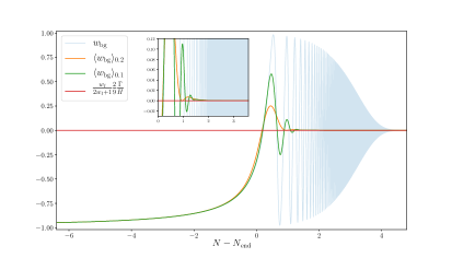
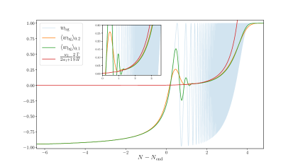
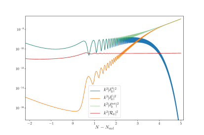
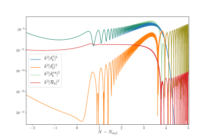
Figure 6: Time evolution of the background equations-of-state parameters (upper panels), with the insets zooming in the regime of validity of the analytical approximation (3.12), as well as scalar perturbations (lower panels), as a function of the number of $e$-folds, in the cases of decay into pressureless matter $w_{\mathrm{f}}=0$ (left panels) and into a stiff fluid $w_{\mathrm{f}}=1$ (right panels). Apart from the value of $w_{\mathrm{f}}$, the setup and parameter values are the same as in all previous figures.

Another way to test this robustness is to study whether the above conclusion is still valid when the inflaton decays into a fluid with an equation of state that differs from the one of radiation. We have therefore considered two additional cases corresponding to a decay into a fluid with $w_{\mathrm{f}}=0$ (pressureless matter) and a decay into a fluid with $w_{\mathrm{f}}=1$ (stiff matter). The results are displayed in Fig. 6 and confirm that our description of the instability generalises to arbitrary equation-of-state parameters $w_{\mathrm{f}}$. On the upper panels, we show the total equations of state $w_{\mathrm{bg}}$ and their averaged values, as well as the analytical approximation Eq. (3.12), as a function of the number of $e$-folds. One verifies that the equation-of-state parameter indeed asymptotes $w_{\mathrm{bg}}=0$ (left panel) and $w_{\mathrm{bg}}=1$ (right panel) at late time. On the lower panels, we have displayed the time evolution of the density contrasts and of the curvature perturbation. The growth $\delta_{k}\propto a$ is still observed until the universe is dominated by the fluid, regardless of its equation of state.

3.3 Radiative decay and PBH formation from metric preheating

In the covariant description developed in Sec. 3, two fluids were necessary to fully describe the scalar field fluctuations. This shows that cosmological inhomogeneities of a scalar field and of a perfect fluid are a priori two very different physical systems, featuring different properties. It is therefore rather intriguing that, during the oscillatory phase, the averaged equation of state is the one of pressureless matter, and that inside the instability band, the density contrast behaves as the one of pressureless matter too, since it grows linearly with the scale factor.

The formation of primordial black holes has mostly been studied in the context of perfect fluids, so if this correspondence between an oscillating scalar field and a pressureless perfect fluid does hold (and even in the presence of additional radiation), it would have important practical consequences [58] for studying the production of PBHs from the metric preheating instability. This is why, in this section, we compare more carefully the behaviour of the cosmological perturbations of the system at hand with those of a single perfect fluid sharing the same equation-of-state parameter.

A key concept in this comparison is the one of the equation of state “felt” by the perturbations, if they are interpreted as perturbations of a single perfect fluid. We start by recalling the behaviour of the density contrast for a perfect fluid with a given equation-of-state parameter $w$. This will allow us to extract the equation-of-state parameter from the time dependence of the density contrast, and to apply this formula to the system studied in Sec. 3 in order to derive the effective “equation of state” felt by the density perturbations. We will then compare it with the equation of state of the background.

In order to implement this program, a remark is in order regarding the definition of the density contrast. So far, we have worked in terms of the density contrast $\delta^{\mathrm{(gi)}}$ (noted $\delta_{\mathrm{g}}$ in LABEL:Bardeen:1980kt), which consists in measuring the energy density relative to the hypersurface which is as close as possible to a “Newtonian” time slicing. However, for a single perfect fluid, this density contrast usually stays constant at large scales and, as a consequence, cannot be used as a tracer of the equation-of-state parameter. Fortunately, as is well-known, there are other possible definitions, in particular $\delta_{\mathrm{com}}$ (noted $\delta_{\mathrm{m}}$ in LABEL:Bardeen:1980kt), which measures the amplitude of energy density from the point of view of matter, and corresponds to the density contrast in the comoving-orthogonal gauge. The behaviour of $\delta_{\mathrm{com}}$ does depend on $w$ on large scales and, therefore, it is a useful quantity for our purpose. The relationship between $\delta^{\mathrm{(gi)}}$ and $\delta_{\mathrm{com}}$ is given by

$$\delta^{\mathrm{(gi)}}=\delta_{\mathrm{com}}-\frac{\rho^{\prime}}{\rho}v^{(\mathrm{gi})}=\delta_{\mathrm{com}}\left[1+3\frac{a^{2}H^{2}}{k^{2}}\left(1+\frac{\Phi^{\prime}}{aH\Phi}\right)\right],$$ (3.27)

which shows that, although they behave differently on super-Hubble scales, their evolution is identical on small scales. To prove this relation, we have used that the density contrast $\delta_{\mathrm{com}}$ is related to the Bardeen potential through the Poisson equation [59]

$$\delta_{\mathrm{com}}=-\frac{2k^{2}M_{\scriptscriptstyle{\mathrm{Pl}}}^{2}}{a^{2}\rho}\Phi\,.$$ (3.28)

If the space-time expansion is driven by a perfect fluid with constant equation-of-state parameter $w$, the energy density scales as $\rho=\rho_{\mathrm{end}}(a_{\mathrm{end}}/a)^{3(1+w)}$, which leads to

$$\delta_{\mathrm{com}}=\delta_{\mathrm{com}}^{\mathrm{end}}\left(\frac{a}{a_{\mathrm{end}}}\right)^{1+3w}\frac{\Phi}{\Phi_{\mathrm{end}}},$$ (3.29)

where the Bardeen potential follows the equation of motion [47]

$$\frac{\mathrm{d}^{2}}{\mathrm{d}(k\eta)^{2}}\left[(k\eta)^{\nu}\Phi\right]+\frac{2}{k\eta}\frac{\mathrm{d}}{\mathrm{d}k\eta}\left[(k\eta)^{\nu}\Phi\right]+\left[w-\frac{\nu(\nu+1)}{\left(k\eta\right)^{2}}\right](k\eta)^{\nu}\Phi=0\,,$$ (3.30)

with $\nu=2/(1+3w)$. The solution to this equation is given by

$$\Phi_{\bm{k}}=(wk\eta)^{\alpha}\left[A_{\bm{k}}J_{\alpha}(wk\eta)+B_{\bm{k}}J_{-\alpha}(wk\eta)\right],$$ (3.31)

with $\alpha=-(5+3w)/[2(1+3w)]$, $J_{\alpha}$ being a Bessel function and $A_{\bm{k}}$, $B_{\bm{k}}$ two integration constants fixed by the initial conditions. The behaviour of this solution depends on whether $|wk\eta|\ll 1$ or $|wk\eta|\gg 1$, i.e. on whether the mode wavelength is larger or smaller than the sound horizon $w/H$.

On super-sonic scales, $|wk\eta|\ll 1$, the Bessel functions can be expanded according to $J_{\alpha}(z)\propto z^{\alpha}$. Since $\alpha<0$ for $w>-1/3$, Eq. (3.31) features a constant mode and a decaying mode. The Bardeen potential thus asymptotes to a constant, and $\delta_{\mathrm{com}}\propto a^{1+3w}$, see Eq. (3.29). If $w=0$, then $\delta_{\mathrm{com}}\propto a$, which is a well-known result.

On sub-sonic scales, $|wk\eta|\gg 1$, the Bessel functions can be expanded according to $J_{\alpha}(z)\simeq\mathchoice{{\hbox{$\displaystyle\sqrt{2/(\pi z)\,}$}\lower 0.4pt\hbox{\vrule height=7.5pt,depth=-6.00003pt}}}{{\hbox{$\textstyle\sqrt{2/(\pi z)\,}$}\lower 0.4pt\hbox{\vrule height=7.5pt,depth=-6.00003pt}}}{{\hbox{$\scriptstyle\sqrt{2/(\pi z)\,}$}\lower 0.4pt\hbox{\vrule height=5.25pt,depth=-4.20003pt}}}{{\hbox{$\scriptscriptstyle\sqrt{2/(\pi z)\,}$}\lower 0.4pt\hbox{\vrule height=3.75pt,depth=-3.00002pt}}}\cos[z-\pi(1+2\alpha)/4]$. This leads to $\delta_{\mathrm{com}}\simeq a^{-1/2+3w/2}\cos[wk\eta-\pi(1+2\alpha)/4]$. The density contrast thus oscillates as a result of the competition between gravity and pressure, and compared to the super-sonic case, the overall amplitude also scales differently with the scale factor. One also notices that this formula cannot be applied if $w=0$. Indeed, in that case, the argument of the Bessel functions vanishes. Physically, if $w=0$, there is no sound horizon anymore (since the pressure vanishes), and all scales are “super-sonic” by definition.

Figure 7: Effective equation-of-state parameters for the perturbations as a function of the number of $e$-folds. When the mode $k$ is super-sonic, its effective equation-of-state parameter is given by $w_{\mathrm{eff}}^{\mathrm{super}}$ (red line), and respectively by $w_{\mathrm{eff}}^{\mathrm{sub}}$ (green line) when it is sub-sonic. In order to facilitate the reading of the figure, the effective equation-of-state parameters are displayed with dashed lines in the regimes where they are not relevant. The instantaneous background equation of state (transparent blue line) and its averaged value (orange line) are also represented for comparison. When $\left\langle w_{\mathrm{bg}}\right\rangle\approx 0$, the sound horizon is very small and the super-sonic effective equation of state (red line) is the relevant one. As expected, it is close to $0$. However when $\left\langle w_{\mathrm{bg}}\right\rangle$ starts to depart from zero, since the physical mode $k/a$ is within the Hubble radius (see Fig. 2), the sub-sonic equation of state (green line) becomes the relevant one and, as expected, it quickly converges to $1/3$. Note however that between these two asymptotic regimes, the effective equation of state for the perturbation does not match the one of the background.

These two limiting expressions of the density contrast can be used to define an effective equation-of-state parameter “felt” by the perturbations. Since $\delta_{\mathrm{com}}\propto a^{1+3w}$ on super-sonic scales, we define

$$w_{\mathrm{eff}}^{\mathrm{super}}\equiv\frac{1}{6}\frac{\mathrm{d}\ln\left(k^{3}\left\langle\delta_{\mathrm{com}}^{2}\right\rangle\right)}{\mathrm{d}\ln a}-\frac{1}{3}\,,$$ (3.32)

where $\langle\cdot\rangle$ stands for time averaging over possible background oscillations. On sub-sonic scales, $\delta_{\mathrm{com}}\simeq a^{-1/2+3w/2}\cos[wk\eta-\pi(1+2\alpha)/4]$, so we introduce

$$w_{\mathrm{eff}}^{\mathrm{sub}}\equiv\frac{1}{3}\frac{\mathrm{d}\ln\left(k^{3}\left\langle\delta_{\mathrm{com}}^{2}\right\rangle\right)}{\mathrm{d}\ln a}+\frac{1}{3}\,.$$ (3.33)

Which of these two effective equations of state is relevant depends on whether the mode $k$ is sub-sonic and super-sonic. In Fig. 7, we display these two quantities, $w_{\mathrm{eff}}^{\mathrm{super}}$ and $w_{\mathrm{eff}}^{\mathrm{sub}}$, from the value of $\delta_{\mathrm{com}}$ numerically obtained as in the previous figures, and compare them with the (averaged) equation-of-state parameter of the background. In all cases, the time averaging is performed with a Gaussian kernel of constant standard deviation given by $0.2$ $e$-folds. Let us also stress again that, on sub-Hubble scales, the density contrast in the comoving-orthogonal gauge, $\delta_{\mathrm{com}}$, coincides with the one in the longitudinal gauge displayed in Figs. 5 and 6.

During the first oscillations, the equation-of-state parameter vanishes (on average) in the background, and recalling that all modes are super-sonic for a vanishing equation-of-state parameter, one can check that the relevant equation of state, $w_{\mathrm{eff}}^{\mathrm{super}}$, indeed vanishes, and that the red and orange curves in Fig. 7 are indeed close. This however lasts for a few $e$-folds only, after which neither of the effective equations of state correctly reproduces the behaviour of the (averaged) equation of state of the background. In addition, for the sub-sonic scales that lie inside the instability band, $\langle w_{\mathrm{bg}}\rangle$ does not coincide at all with $w_{\mathrm{eff}}^{\mathrm{sub}}$ during the oscillating phase until radiation strongly dominates the universe content and both converge to $1/3$. Therefore, despite the fact that the inflaton background effectively behaves as pressureless matter on average, and that its decay product is a perfect fluid, the perturbations of the system are not those of perfect fluids. This confirms that the system made of a decaying, oscillating scalar field has different behaviour from a pure perfect fluid, and cannot be simply modelled as such.

Let us note that this fundamental difference is even more striking in the case where the inflaton potential is quartic close to its minimum, since in that case the correspondence between the inflaton perturbations and those of a perfect fluid with the same background equation of state breaks down even in the absence of inflaton radiative decay. As shown in LABEL:Jedamzik:2010dq indeed, while $\langle w_{\mathrm{bg}}\rangle=1/3$ in such a case, the instability of metric preheating is still present, and the density contrast grows even faster than that of pressureless matter (namely, exponentially with the scale factor) in the instability band, while the density contrast for a perfect fluid having $w=1/3$ is constant on sub-sonic scales.

As mentioned above, this implies that, in order to study the production of PBHs that arises from the increase of the density contrast in the instability band, one cannot rely on techniques developed for perfect fluids. In LABEL:Carr:2018nkm for instance, it was used that an overdensity of a perfect fluid with constant equation-of-state parameter $w$ collapses into a black hole if it exceeds the critical density contrast [62, 63]

$$\delta_{\mathrm{c}}=\frac{3(1+w)}{5+3w}\sin^{2}\left(\frac{\pi\mathchoice{{\hbox{$\displaystyle\sqrt{w\,}$}\lower 0.4pt\hbox{\vrule height=4.30554pt,depth=-3.44446pt}}}{{\hbox{$\textstyle\sqrt{w\,}$}\lower 0.4pt\hbox{\vrule height=4.30554pt,depth=-3.44446pt}}}{{\hbox{$\scriptstyle\sqrt{w\,}$}\lower 0.4pt\hbox{\vrule height=3.01389pt,depth=-2.41113pt}}}{{\hbox{$\scriptscriptstyle\sqrt{w\,}$}\lower 0.4pt\hbox{\vrule height=2.15277pt,depth=-1.72223pt}}}}{1+3w}\right)\,,$$ (3.34)

in which $w$ was replaced with $w\sim\Gamma/H$ [see Eq. (3.12)]. If $w=0$, Eq. (3.34) indicates that any local overdensity ends up forming a black hole, which is indeed the case in the absence of any pressure force. The analysis of LABEL:Carr:2018nkm thus suggests that what limits the formation of PBHs from the instability of metric preheating is the presence of (even small amounts of) radiation, which provide a non-vanishing value to the equation-of-state parameter, and hence to $\delta_{\mathrm{c}}$. However, the results of the present work cast some doubt on such a treatment since we showed that an oscillating scalar field decaying into a radiation fluid cannot be treated as a collection of perfect fluids at the perturbed level [furthermore, the background equation of state for such a system is strongly time dependent, see Eq. (3.12), while Eq. (3.34) only applies to constant equation-of-state parameters].

In LABEL:Martin:2019nuw, the formation of PBHs from the overdensities of an oscillating scalar field was studied in the context of metric preheating, and it was found that what limits the formation of PBHs is rather the fact that the instability does not last for ever, since it stops when radiation takes over. Indeed, although it is true that any overdensity inside the instability band develops towards forming a black hole, the amount of time needed for a black hole to form depends on (and decreases with) the initial value of the density contrast. By requiring that it takes less time than what is available before the complete inflaton decay (which, as we have established in Sec. 3.2, signals the end of the instability phase that is otherwise not affected by the presence of radiation being produced), one obtains a lower bound on the density contrast, which however has nothing to do with Eq. (3.34).

4 Conclusions

Preheating effects are often believed to be observationally irrelevant in single-field models of inflation. Although this is true at large scales, where the curvature perturbation is merely conserved, the situation is different at small scales, namely those leaving the Hubble radius a few $e$-folds before the end of inflation. Such scales are subject to a persistent instability proceeding in the narrow-resonance regime [35], which causes the density contrast to grow, leading to various possible effects such as early structure formation or even PBHs formation [40].

In contrast to the case of background preheating, where the narrow-resonance regime is irrelevant since, in a time-dependent background, the system spends very little time in the thin instability band and the resonance effects are wiped out, in the metric preheating case, the presence of the instability is actually caused by cosmic expansion itself (see Fig. 2). This is the reason why this mechanism is both atypical and very efficient.

This fact was known to be true [35] only if the inflaton is uncoupled to other degrees of freedom. However, in order for reheating to proceed, the inflaton field must decay into radiation, and the goal of this paper was to determine whether this decay could spoil the instability. Using the formalism of cosmological perturbations in the presence of interactions between fluids, we have shown that it is not the case, and that the growth of the density contrast inside the instability band remains unaffected until the radiation fluid dominates the universe content.

We have also stressed that there is a fundamental difference between the cosmological perturbations of an oscillating scalar field and those of a perfect fluid, and that techniques developed to study the formation of PBHs from perfect fluid overdensities cannot be applied to the present context. Instead, a dedicated analysis such as the one of LABEL:Martin:2019nuw must be performed. Our results have confirmed that the presence of radiation can simply be ignored until it comes to dominate the energy budget, thus stopping the instability.

The results of this work therefore confirm that the instability of metric preheating is unavoidable in single-field models of inflation, since it only requires an oscillating scalar field in a cosmological background, which is the state of the universe at the end of most inflationary models, and given that it is robust against perturbative decay of this field.

References

- [1] A. A. Starobinsky, A New Type of Isotropic Cosmological Models Without Singularity, Phys. Lett. B91 (1980) 99–102.
- [2] A. H. Guth, The Inflationary Universe: A Possible Solution to the Horizon and Flatness Problems, Phys.Rev. D23 (1981) 347–356.
- [3] A. D. Linde, A New Inflationary Universe Scenario: A Possible Solution of the Horizon, Flatness, Homogeneity, Isotropy and Primordial Monopole Problems, Phys.Lett. B108 (1982) 389–393.
- [4] A. Albrecht and P. J. Steinhardt, Cosmology for Grand Unified Theories with Radiatively Induced Symmetry Breaking, Phys.Rev.Lett. 48 (1982) 1220–1223.
- [5] A. D. Linde, Chaotic Inflation, Phys.Lett. B129 (1983) 177–181.
- [6] A. Albrecht, P. J. Steinhardt, M. S. Turner and F. Wilczek, Reheating an Inflationary Universe, Phys. Rev. Lett. 48 (1982) 1437.
- [7] A. D. Dolgov and A. D. Linde, Baryon Asymmetry in Inflationary Universe, Phys. Lett. 116B (1982) 329.
- [8] L. F. Abbott, E. Farhi and M. B. Wise, Particle Production in the New Inflationary Cosmology, Phys. Lett. 117B (1982) 29.
- [9] M. S. Turner, Coherent Scalar Field Oscillations in an Expanding Universe, Phys. Rev. D28 (1983) 1243.
- [10] Y. Shtanov, J. H. Traschen and R. H. Brandenberger, Universe reheating after inflation, Phys. Rev. D51 (1995) 5438–5455, [hep-ph/9407247].
- [11] L. Kofman, A. D. Linde and A. A. Starobinsky, Reheating after inflation, Phys. Rev. Lett. 73 (1994) 3195–3198, [hep-th/9405187].
- [12] L. Kofman, A. D. Linde and A. A. Starobinsky, Towards the theory of reheating after inflation, Phys. Rev. D56 (1997) 3258–3295, [hep-ph/9704452].
- [13] B. A. Bassett, S. Tsujikawa and D. Wands, Inflation dynamics and reheating, Rev. Mod. Phys. 78 (2006) 537–589, [astro-ph/0507632].
- [14] M. A. Amin, M. P. Hertzberg, D. I. Kaiser and J. Karouby, Nonperturbative Dynamics Of Reheating After Inflation: A Review, Int. J. Mod. Phys. D24 (2014) 1530003, [1410.3808].
- [15] V. F. Mukhanov and G. Chibisov, Quantum Fluctuation and Nonsingular Universe., JETP Lett. 33 (1981) 532–535.
- [16] H. Kodama and M. Sasaki, Cosmological Perturbation Theory, Prog. Theor. Phys. Suppl. 78 (1984) 1–166.
- [17] Planck collaboration, Y. Akrami et al., Planck 2018 results. I. Overview and the cosmological legacy of Planck, 1807.06205.
- [18] Planck collaboration, Y. Akrami et al., Planck 2018 results. X. Constraints on inflation, 1807.06211.
- [19] J. Martin, C. Ringeval and V. Vennin, Encyclopaedia Inflationaris, Phys. Dark Univ. 5-6 (2014) 75–235, [1303.3787].
- [20] J. Martin, C. Ringeval, R. Trotta and V. Vennin, The Best Inflationary Models After Planck, JCAP 1403 (2014) 039, [1312.3529].
- [21] J. Martin, The Observational Status of Cosmic Inflation after Planck, Astrophys. Space Sci. Proc. 45 (2016) 41–134, [1502.05733].
- [22] D. Chowdhury, J. Martin, C. Ringeval and V. Vennin, Inflation after Planck: Judgment Day, 1902.03951.
- [23] F. Finelli and R. H. Brandenberger, Parametric amplification of gravitational fluctuations during reheating, Phys. Rev. Lett. 82 (1999) 1362–1365, [hep-ph/9809490].
- [24] J. Martin and C. Ringeval, Inflation after WMAP3: Confronting the Slow-Roll and Exact Power Spectra to CMB Data, JCAP 0608 (2006) 009, [astro-ph/0605367].
- [25] V. Vennin, J. Martin and C. Ringeval, Cosmic Inflation and Model Comparison, Comptes Rendus Physique (2015) .
- [26] J. Martin and C. Ringeval, First CMB Constraints on the Inflationary Reheating Temperature, Phys.Rev. D82 (2010) 023511, [1004.5525].
- [27] J. Martin, C. Ringeval and V. Vennin, Observing Inflationary Reheating, Phys. Rev. Lett. 114 (2015) 081303, [1410.7958].
- [28] J. Martin, C. Ringeval and V. Vennin, Information Gain on Reheating: the One Bit Milestone, 1603.02606.
- [29] R. J. Hardwick, V. Vennin, K. Koyama and D. Wands, Constraining Curvatonic Reheating, JCAP 1608 (2016) 042, [1606.01223].
- [30] B. A. Bassett and F. Viniegra, Massless metric preheating, Phys. Rev. D62 (2000) 043507, [hep-ph/9909353].
- [31] B. A. Bassett, F. Tamburini, D. I. Kaiser and R. Maartens, Metric preheating and limitations of linearized gravity. 2., Nucl. Phys. B561 (1999) 188–240, [hep-ph/9901319].
- [32] K. Jedamzik and G. Sigl, On metric preheating, Phys. Rev. D61 (2000) 023519, [hep-ph/9906287].
- [33] F. Finelli and R. H. Brandenberger, Parametric amplification of metric fluctuations during reheating in two field models, Phys. Rev. D62 (2000) 083502, [hep-ph/0003172].
- [34] R. Allahverdi, R. Brandenberger, F.-Y. Cyr-Racine and A. Mazumdar, Reheating in Inflationary Cosmology: Theory and Applications, Ann. Rev. Nucl. Part. Sci. 60 (2010) 27–51, [1001.2600].
- [35] K. Jedamzik, M. Lemoine and J. Martin, Collapse of Small-Scale Density Perturbations during Preheating in Single Field Inflation, JCAP 1009 (2010) 034, [1002.3039].
- [36] R. Easther, R. Flauger and J. B. Gilmore, Delayed Reheating and the Breakdown of Coherent Oscillations, JCAP 1104 (2011) 027, [1003.3011].
- [37] K. Jedamzik, M. Lemoine and J. Martin, Generation of gravitational waves during early structure formation between cosmic inflation and reheating, JCAP 1004 (2010) 021, [1002.3278].
- [38] B. J. Carr and S. W. Hawking, Black holes in the early Universe, Mon. Not. Roy. Astron. Soc. 168 (1974) 399–415.
- [39] B. J. Carr, The Primordial black hole mass spectrum, Astrophys. J. 201 (1975) 1–19.
- [40] J. Martin, T. Papanikolaou and V. Vennin, Primordial black holes from the preheating instability, 1907.04236.
- [41] M. Khlopov, B. Malomed and I. Zeldovich, Gravitational instability of scalar fields and formation of primordial black holes, Mon. Not. Roy. Astron. Soc. 215 (1985) 575–589.
- [42] B. A. Bassett and S. Tsujikawa, Inflationary preheating and primordial black holes, Phys. Rev. D63 (2001) 123503, [hep-ph/0008328].
- [43] T. Suyama, T. Tanaka, B. Bassett and H. Kudoh, Black hole production in tachyonic preheating, JCAP 0604 (2006) 001, [hep-ph/0601108].
- [44] M. Abramowitz and I. A. Stegun, Ch. 20 in Handbook of mathematical functions with formulas, graphs, and mathematical tables. National Bureau of Standards, Washington, US, ninth ed., 1970.
- [45] G. N. Felder, J. Garcia-Bellido, P. B. Greene, L. Kofman, A. D. Linde and I. Tkachev, Dynamics of symmetry breaking and tachyonic preheating, Phys. Rev. Lett. 87 (2001) 011601, [hep-ph/0012142].
- [46] M. Desroche, G. N. Felder, J. M. Kratochvil and A. D. Linde, Preheating in new inflation, Phys. Rev. D71 (2005) 103516, [hep-th/0501080].
- [47] V. F. Mukhanov, H. Feldman and R. H. Brandenberger, Theory of cosmological perturbations. Part 1. Classical perturbations. Part 2. Quantum theory of perturbations. Part 3. Extensions, Phys. Rept. 215 (1992) 203–333.
- [48] K. D. Lozanov and M. A. Amin, Self-resonance after inflation: oscillons, transients and radiation domination, Phys. Rev. D 97 (2018) 023533, [1710.06851].
- [49] D. Maity and P. Saha, (P)reheating after minimal Plateau Inflation and constraints from CMB, JCAP 07 (2019) 018, [1811.11173].
- [50] K. A. Malik and D. Wands, Adiabatic and entropy perturbations with interacting fluids and fields, JCAP 0502 (2005) 007, [astro-ph/0411703].
- [51] K.-Y. Choi, J.-O. Gong and D. Jeong, Evolution of the curvature perturbation during and after multi-field inflation, JCAP 0902 (2009) 032, [0810.2299].
- [52] K. A. Malik and D. Wands, Cosmological perturbations, Physics Reports 475 (May, 2009) 1–51.
- [53] G. Leung, E. R. M. Tarrant, C. T. Byrnes and E. J. Copeland, Reheating, Multifield Inflation and the Fate of the Primordial Observables, JCAP 1209 (2012) 008, [1206.5196].
- [54] G. Leung, E. R. M. Tarrant, C. T. Byrnes and E. J. Copeland, Influence of Reheating on the Trispectrum and its Scale Dependence, JCAP 1308 (2013) 006, [1303.4678].
- [55] I. Huston and A. J. Christopherson, Isocurvature Perturbations and Reheating in Multi-Field Inflation, 1302.4298.
- [56] L. Visinelli, Cosmological perturbations for an inflaton field coupled to radiation, JCAP 1501 (2015) 005, [1410.1187].
- [57] J. Martin and L. Pinol, In preparation, .
- [58] B. Carr, K. Dimopoulos, C. Owen and T. Tenkanen, Primordial Black Hole Formation During Slow Reheating After Inflation, Phys. Rev. D97 (2018) 123535, [1804.08639].
- [59] J. M. Bardeen, Gauge Invariant Cosmological Perturbations, Phys. Rev. D22 (1980) 1882–1905.
- [60] C.-M. Yoo, T. Harada, J. Garriga and K. Kohri, Primordial black hole abundance from random Gaussian curvature perturbations and a local density threshold, PTEP 2018 (2018) 123E01, [1805.03946].
- [61] S. Young, C. T. Byrnes and M. Sasaki, Calculating the mass fraction of primordial black holes, JCAP 1407 (2014) 045, [1405.7023].
- [62] T. Harada, C.-M. Yoo and K. Kohri, Threshold of primordial black hole formation, Phys. Rev. D88 (2013) 084051, [1309.4201].
- [63] T. Harada, C.-M. Yoo, K. Kohri and K.-I. Nakao, Spins of primordial black holes formed in the matter-dominated phase of the Universe, Phys. Rev. D 96 (2017) 083517, [1707.03595].