Using expectile regression for classification ratemaking

Abstract

Calculating the risk premium is a prime objective in non-life actuarial science. This paper examines an application of expectile regression to determine risk premium rates for tariff classes. A so-called Expectile Premium Principle that inherits the good statistical properties of the expectile regression is investigated. This new premium principle as a coherent risk measure can give more information about the shape of the entire loss distribution. For model comparison, we consider the conventional GLMs and three quantile regression models discussed in Heras et al. (2018) and Baione and Biancalana (2019, 2020) as the benchmarks. A simulation study is designed to evaluate the model performance. Based on a real world automobile insurance data set, our experimental result reveals the expectile regression with Expectile Premium Principle has the advantage of better differentiating the heterogeneity among tariff classes and also has a greater ability to distinguish high risks from low risks.

Keywords: risk loading; expectile regression; quantile regression; Expectile Premium Principle; coherent risk measure


Compiled date: March 13, 2024

1 Introduction

In a highly competitive insurance market, one of the most important objectives for actuaries is to determine appropriate risk premiums for tariff classes (the policyholders with similar risks are classified into the same tariff class based on various risk factors). The risk premium usually involves a separate analysis of two parts: pure premium and risk loading. The former corresponds to the expected value of future losses and the latter is supporting the insurer’s ability to cover additional losses caused by the unfavorable deviation. While a rich variety of literature on classification ratemaking methods has proposed how to predict the pure premium (Yang et al. (2018), Smyth and Jørgensen (2002), Henckaerts et al. (2018), among others), the statistical estimation of the risk loading has received much less attention, especially in the presence of additional covariate information. To estimate the risk loading correctly and at the same time allow classification by tariff features, we develop a new statistical framework to predict risk premiums of individual policies based on an arbitrary set of risk factors.

In order to determine the risk premium for a individual risk, many different premium principles have been proposed in actuarial science. The most common approach in ratemaking for tariff classes is to apply the Expected Value Premium Principle (EVPP) or the Standard Deviation Premium Principle (SDPP), in which the pure premium is based on conventional generalized linear models (GLMs) and the risk loading can be expressed as a certain percentage of the expectation or the standard deviation of the losses. An alternative method is to apply a distortion function as a premium principle, from which the risk premium is calculated on the basis of the loss distribution, e.g., Wang Premium Principle (Wang, 2000) and Value-at-risk (VaR) Premium Principle (Kudryavtsev, 2009). The VaR Premium Principle is based on quantile regression model when a set of risk factors are considered. It explains the needs of risk loading quite well, as it estimates the maximum possible losses that an individual policy may incur with a given probability $1-\tau$ during the forecasting period, in which the risk loading is expressed as the difference between the $\tau$-th quantile and $50\%$-th quantile. Compared with GLMs used in the EVPP and SDPP, quantile regression used in VaR Premium Principle shows excellent statistical properties and can better explain the tail characteristics of a response variable’s conditional distribution given the values of one or more covariates (Koenker and Bassett Jr, 1978). The parameter estimation is less affected by outliers, and the estimation result is more robust (Gilchrist, 2000). More recently, Heras et al. (2018) propose a so-called Quantile Premium Principle (QPP) based on quantile regression, in which the risk loading is adjusted by a risk loading parameter compared with the VaR Premium Principle. Baione and Biancalana (2019) propose an alternative quantile regression by using a Two-Part Quantile Premium Principle (TSQPP) . However, the drawback is that the traditional quantile regression may suffer from the problem of quantile crossing, which may particularly occur at extreme quantiles when the data are rare (Dong et al., 2015). To obviate this problem, Baione and Biancalana (2020) suggest applying a more parsimonious approach to calculate the risk premium based on the parametric quantile regression (PQR) model introduced by Frumento and Bottai (2016, 2017). PQR models the regression coefficients as parametric functions of the quantile level, which expands the potential of quantile modelling and avoids the problem of over-parameterization and time-consumption. Table 1 gives an overview of model specifications and various premium principles discussed in existing classification ratemaking research.

Quantile regression is still quite limiting in the ratemaking process, since the use of VaR as a risk measure is not without criticism (Xie et al., 2014). First, it lacks subadditivity, which contradicts the conventional rule of risk diversification. Second, VaR is insensitive to the magnitude of the loss as it depends only on the probabilities of extreme events but not on their values. This suggests that VaR with a given tail probability may not always be an appropriate risk measure when insurers and regulators are concerned with extreme claims. Third, VaR conveys only a small slice of the loss distribution information as it focuses exclusively on the upper tail of the distribution. To avoid the aforementioned problems with VaR, Kuan et al. (2009) propose an expectile-based VaR as an alternative to the VaR as a downside risk measure in the stock market. The $\tau$-th expectile is defined as the solution to the minimization of asymmetrically weighted mean squared errors, with the weights $\tau$ and $1-\tau$ assigned to positive and negative deviations, respectively. Comparing to the $L_{1}$ norm used in quantile, expectile which utilizes the $L_{2}$ norm is more sensitive to extreme values of the loss distribution. Meanwhile, the expectile provides a more smooth surface in the direction of $\tau$, which leads to expectile estimates behaving more stable even for very small or very large values of $\tau$. The estimator in expectile is also asymptotically unbiased and normal while the properties of asymptotic unbiasedness and normality are not guaranteed in quantile (Waltrup et al., 2015). Moreover, expectile is determined by tail expectations rather than tail probabilities, thus providing more information about the tails. Considering expectile as an example of shortfall risk measures is also known as zero-utility premia in the actuarial literature (Föllmer and Schied, 2002), expectile can be regarded as a perfectly reasonable alternative to quantile as it depends on both the tail realizations and their probabilities and defines a coherent risk measure for $\tau\geq\frac{1}{2}$ (Bellini et al., 2014). In addition, when dealing with heterogeneous data in regression, different types of covariates can be introduced in expectile regression models via parametric, semiparametric and nonparametric method which are fully discussed in statistical and financial literature (Kuan et al. (2009), Yao and Tong (1996), Sobotka et al. (2013), Xie et al. (2014), among others) Thus, this regression setting can provide a very nice statistical modelling framework for classification ratemaking in non-life actuarial science.

Combining insights from both expectile regression and the actuarial science literature, our main contribution is the design of an efficient premium principle called Expectile Premium Principle (EPP) based on expectile regression, suitable for determining appropriate tariff class risk premium rates . The EPP is similar to the QPP discussed in Heras et al. (2018) and Baione and Biancalana (2020), but can satisfy all four properties of a coherent risk measure (i.e., translation invariance, monotonicity, positive homogeneity and subadditivity). Besides the GLMs and several quantile regressions used as the benchmarks, including QR (Heras et al., 2018), QRII (Baione and Biancalana, 2019) and PQR models (Baione and Biancalana, 2020), we design a simulation study to evaluate the model performance of all competing models. Based on a real world automobile insurance data set, our empirical result shows the proposed method can overcome quantile regression drawbacks and prevent efficiency loss in the estimation of risk premiums. It also has the advantage of better differentiating the heterogeneity among tariff classes and also has a greater ability to distinguish high risks from low risks. To the best of our knowledge, this is the first time that the expectile regression has been implemented into the process of classification ratemaking.

The remainder of the article is structured as follows. Section 2 provides a brief description of the standard GLMs and several quantile regressions for classification ratemaking. Section 3 describes the proposed Expectile Premium Principle based on expectile regression. A simulation study is conducted in Section 4. A numerical application and comparative study are discussed in Section 5. Section 6 concludes this study with suggestions for further research. The data and R code can be found at https://github.com/lizhengxiao/expectile-regression-risk-loading.

[b] Ratemaking models Premium Principle Risk premium References Risk loading Risk loading parameter GLMs Expected value Premium Principle (EVPP) $H\left({{Y}_{i}}\right)=\mathbb{E}\left({{Y}_{i}}\right)+\varphi\mathbb{E}\left({{Y}_{i}}\right)$ Heras et al. (2018) $\varphi\mathbb{E}\left({{Y}_{i}}\right)$ $\varphi$ GLMs Standard deviation Premium Principle (SDPP) $H\left({{Y}_{i}}\right)=\mathbb{E}\left({{Y}_{i}}\right)+\varphi\sqrt{\text{Var}\left({{Y}_{i}}\right)}$ Heras et al. (2018) $\varphi\sqrt{\text{Var}\left({{Y}_{i}}\right)}$ $\varphi$ QR* VaR Premium Principle $H\left({{Y}_{i}}\right)={{Q}_{{{Y}_{i}}}}\left(\tau\right)=\inf\left\{u\in\mathbb{R}:\ {{F}_{{{Y}_{i}}}}\left(u\right)\geq\tau\right\}$ Kudryavtsev (2009) ${{Q}_{{{Y}_{i}}}}\left(\tau\right)-\mathbb{E}\left({{Y}_{i}}\right)$ $\tau$ QR Quantile Premium Principle (QPP) $H\left({{Y}_{i}}\right)=\mathbb{E}\left({{Y}_{i}}\right)+\varphi\left[{{Q}_{{{Y}_{i}}}}\left(\tau\right)-\mathbb{E}\left({{Y}_{i}}\right)\right]$ Heras et al. (2018) $\varphi\left[{{Q}_{{{Y}_{i}}}}\left(\tau\right)-\mathbb{E}\left({{Y}_{i}}\right)\right]$ $\varphi(\tau=95\%)$ QRII Two-part quantile Premium Principle (TSQPP) $H\left({{Y}_{i}}\right)=\left(1-{{p}_{i}}\right){{Q}_{Y_{i}^{*}}}\left(\tau\right)$ Baione and Biancalana (2019) $\left(1-{{p}_{i}}\right){{Q}_{Y_{i}^{*}}}\left(\tau\right)-\mathbb{E}\left({{Y}_{i}}\right)$ $\tau$ PQR Quantile Premium Principle (QPP) $H\left({{Y}_{i}}\right)=\mathbb{E}\left({{Y}_{i}}\right)+\varphi\left[{{Q}_{{{Y}_{i}}}}\left(\tau\right)-\mathbb{E}\left({{Y}_{i}}\right)\right]$ Baione and Biancalana (2020) $\varphi\left[{{Q}_{{{Y}_{i}}}}\left(\tau\right)-\mathbb{E}\left({{Y}_{i}}\right)\right]$ $\varphi(\tau=95\%)$

• Notes: Assuming that random variable ${{Y}_{i}}$ denotes the aggregate claim amount for individual policy $i,i=1,\dots,N$, the risk premium of policy $i$ can be expressed as a distortion function $H\left({{Y}_{i}}\right)$ of the random variable ${{Y}_{i}}$.

• In the EVPP, the risk premium equals the pure premium plus a percentage of the pure premium. $\varphi>0$ denotes the risk loading parameter and $\varphi\mathbb{E}\left({{Y}_{i}}\right)$ denotes the corresponding risk loading.

• In the SDPP, the risk premium equals the pure premium plus a percentage of the standard deviation, $\varphi>0$ denotes the risk loading parameter and $\varphi\sqrt{\text{Var}\left({{Y}_{i}}\right)}$ denotes the corresponding risk loading.

• In the VaR Premium Principle, ${{Q}_{{{Y}_{i}}}}\left(\tau\right)$ denotes the $\tau$-th quantile of the aggregate claim amount, thus the risk premium is calculated as a quantile of the aggregate claim amount of an individual policy. $\tau$ denotes the risk loading parameter.

• In the QPP, $\varphi$ is the risk loading parameter, and $\varphi\left[{{Q}_{{{Y}_{i}}}}\left(\tau\right)-\mathbb{E}\left({{Y}_{i}}\right)\right]$ represents the risk loading, which is the difference between the $\tau$-th quantile of the aggregate claim amount and the pure premium. The main difference between the VaR Premium Principle and the QPP is that the risk loading in the QPP is adjusted by risk loading parameter $\varphi$. In the QPP, the authors use the pre-determined $\tau=95\%$ and remain $\varphi$ to be estimated.

• In the TSQPP, $1-{{p}_{i}}$ denotes the probability of incurring at least one claim. The estimation of risk premium is decomposed between a claim probability that indicates whether the policy has claimed, and a quantile of the claim that has incurred at least one claim $Q_{Y_{i}^{*}(\tau)}$, where $Y_{i}^{*}=Y_{i}|Y_{i}>0$.

• In the PQR, parametric quantile regression is used instead of quantile regression model.

Table 1: Literature review about risk premium prediction based on various Premium Principles.

2 The existing ratemaking approaches

This section gives an overview of current classification ratemaking literature, including GLMs and three quantile regression models.

Suppose an insurance portfolio contains $N$ policies, ${{R}_{i}}$ indicates whether or not policy $i$ has a claim submitted, ${{Y}_{i}}$ represents its aggregate claim amount, ${{w}_{i}}$ denotes its exposure, and ${{\bm{x}}_{i}}$ stands for a vector of covariates $(i=1,\cdots,N)$.

2.1 Risk premium estimation via GLMs

To set the premium for individual policyholders, it is a common practice to separate claim probability and non-zero aggregate claim amount, in which the claim probability component models the probability that a given policy incurs claims, and the non-zero component models the aggregate claim amount given that at least one claim has been incurred (Frees, 2009, Frees et al., 2013). Such a decomposition method is commonly called the two-part GLMs framework. In two-part GLMs, for claim probability we assume that $R_{i}$ follows the binomial distribution with parameter $1-p_{i}$, and consider the conventional logistic regression model:

$$\text{logit}\left[\frac{1-{{p}_{i}}}{{{w}_{i}}}\right]=\bm{x}^{\prime}_{i}\bm{\alpha},$$ (1)

where $R_{i}=0$ denotes the policy having no claims with probability $p_{i}$, $\text{logit}(t)=\log\left({t}/{(1-t)}\right)$ is the logit function, $\bm{x}_{i}=(1,x_{i1},\cdots,x_{ik})$ represents the $(k+1)$-dimensional vector of covariates, and $\bm{\alpha}=({{\alpha}_{0}},{{\alpha}_{1}},\cdots,{{\alpha}_{k}}{)}$ denotes the corresponding regression coefficients to be estimated. The left-hand side of (1) is the log odds ratio per exposure, and is corrected for risk exposure ${{w}_{i}}$ (De Jong et al., 2008). Correspondingly, the probability of at least one claim occurring can be obtained by $1-{{p}_{i}}={{w}_{i}}\frac{\exp(\bm{x}^{\prime}_{i}\bm{\alpha})}{1+\exp(\bm{x}^{\prime}_{i}\bm{\alpha})}$. For the non-zero aggregate claim amount, we employ Gamma (GA) regression to model the skewness and heavy tail. The log link function is considered (Kudryavtsev, 2009), and the expected claim amount can be obtained by

$$\log({{\mu}_{i}})=\bm{x}^{\prime}_{i}\bm{\beta},$$ (2)

where $\bm{\beta}=({{\beta}_{0}},{{\beta}_{1}},\cdots,{{\beta}_{k}}{)}$ denotes the corresponding regression coefficients to be estimated in the non-zero claim amount component.

The pure premium of policy $i$ in the two-part GLMs is expressed as the expected value of the aggregate claim amount, which is given by

$$\mathbb{E}\left[{{Y}_{i}}|\bm{x}_{i}\right]=\left(1-{{p}_{i}}\right){{\mu}_{i}}$$ (3)

thus resulting in the risk premium by applying the EVPP and SDPP given respectively by:

$$H\left({Y}_{i}|\bm{x}_{i}\right) =\mathbb{E}\left({{Y}_{i}}|\bm{x}_{i}\right)+\varphi\mathbb{E}\left({{Y}_{i}}|\bm{x}_{i}\right),$$ (4)

$$H\left({{Y}_{i}}|\bm{x}_{i}\right) =\mathbb{E}\left({{Y}_{i}}|\bm{x}_{i}\right)+\varphi\sqrt{\text{Var}\left({{Y}_{i}}|\bm{x}_{i}\right)},$$ (5)

where $\varphi$ is the risk loading parameter.

2.2 Risk premium estimation via QR, QRII and PQR

Similar to the two-part GLMs, an alternative method for modelling the non-zero aggregate claim amount is to apply quantile regression. As aforementioned, three models (i.e., QR, QRII and PQR) are discussed in existing literature, where two different premium principles (i.e., QPP and TSQPP) are employed, see Table 1 for more details.

For QR model, we follow the general guidelines for classification analysis in the risk premium prediction context as proposed in Heras et al. (2018) based on QPP, thus resulting in the risk premium of policy $i$ simply given by

$$H\left({{Y}_{i}}|\bm{x}_{i}\right)=\mathbb{E}(Y_{i}|\bm{x}_{i})+\varphi\left[{{Q}_{{{Y}_{i}}}}\left(\tau|\bm{x}_{i}\right)-\mathbb{E}\left({{Y}_{i}}|\bm{x}_{i}\right)\right],$$ (6)

where ${{\bm{x}}_{i}}$ stands for a vector of covariates, $\mathbb{E}(Y_{i}|\bm{x}_{i})$ is the pure premium obtained by GLMs, and ${{Q}_{{{Y}_{i}}}}\left(\tau|\bm{x}_{i}\right)$ represents the VaR with $\tau$-level. (6) refers to the Quantile Premium Principle (QPP), in which the individual risk premium is a weighted average of pure premium and the $\tau$-level quantile of $Y_{i}$. In Heras et al. (2018), $\tau$ is set to be $95\%$ and $\varphi$ is denoted by the risk loading parameter. In order to estimate the $\tau$-quantile of $Y_{i}$, we can estimate the $\tau_{i}^{*}$-th quantile of $Y_{i}^{*}$, where $Y_{i}^{*}={{Y}_{i}}|{{Y}_{i}}>0$ represents the non-zero aggregate claim amount given that policy $i$ incurs at least one claim, with the following relationship: $\tau_{i}^{*}=({\tau-{{p}_{i}}})/({1-{{p}_{i}}})$ . This ratemaking framework refers to a two-part quantile regression because the probability of having no claim is estimated using the logistic regression model; the non-zero claim amount is modeled by quantile regression. Considering the log link function is quite popular as it is well connected with the multiplicative framework, the covariates can be introduced into log-transformed quantile as follows:

$$\log{{Q}_{Y_{i}^{*}}}\left({{\tau_{i}^{*}}}\left|\bm{x}_{i}\right.\right)=\bm{x}^{\prime}_{i}{{\bm{\gamma}}^{\tau_{i}^{*}}}.$$ (7)

Here we refer ${{Q}_{Y_{i}^{*}}}\left({{\tau_{i}^{*}}}\left|\bm{x}_{i}\right.\right)$ to the VaR at quantile level ${\tau_{i}^{*}}$. In their studies, the response variable is the log-transformed non-zero aggregate claim amounts of individual policies that submit at least one claim. The vectors of regression coefficients $\bm{\gamma}^{\tau_{i}^{*}}=(\gamma_{0}^{\tau_{i}^{*}},\gamma_{1}^{\tau_{i}^{*}},\cdots,\gamma_{k}^{\tau_{i}^{*}})$ are not the same for tariff classes because of their different quantile levels, which indicates its application requires the calibration of a number of quantile regression models on different quantile levels equal to the number of risk classes. Regression coefficients estimation can be derived by solving the following minimization problem with R package quantreg: Quantile Regression; see Koenker and Hallock (2001) for more details.

PQR as the second model considered in our analysis expresses the regression coefficients as some parametric functions of the quantile level (Baione and Biancalana, 2020). This model has several advantages, including parsimony, efficiency, and simple interpretation. PQR results are associated with the choice of the quantile level function. In practice, the choice of the function must ensure that the quantile is monotonically increasing. For instance, polynomials, splines, trigonometric functions, and quantile functions of standard normal distributions could be used. Here we choose a polynomial function to capture the relationship between quantile levels and the coefficients of the quantile regression model. The covariates can be introduced into a log-transformation quantile given by

$$\log{{Q}_{Y_{i}^{*}}}\left({\tau_{i}^{*}}|\bm{x}_{i}\right) =\bm{x}_{i}^{\prime}\bm{\gamma}\left({\tau_{i}^{*}}\left|\bm{\theta}\right.\right),$$

$${{\gamma}_{j}}({\tau_{i}^{*}}|\bm{\theta}) ={{\theta}_{0j}}+{{\theta}_{1j}}{\tau_{i}^{*}}+{{\theta}_{2j}}{\tau_{i}^{*}}^{2},\quad j=0,1,\cdots,k,$$ (8)

where $\bm{\gamma}\left({\tau_{i}^{*}}\left|\bm{\theta}\right.\right)={{\left({{\gamma}_{0}}\left({\tau_{i}^{*}}\left|\bm{\theta}\right.\right),\cdots,{{\gamma}_{k}}\left({\tau_{i}^{*}}\left|\bm{\theta}\right.\right)\right)}}$ denotes the corresponding vector as a function of quantile level ${\tau_{i}^{*}}$ conditioning on finite-dimensional parameters $\bm{\theta}$, and ${{\gamma}_{j}}\left({\tau_{i}^{*}}\right)$ is a polynomial function. We also refer ${{Q}_{Y_{i}^{*}}}\left({\tau_{i}^{*}}|\bm{x}_{i}\right)$ to the VaR at ${\tau_{i}^{*}}$-level. The estimation procedure can be implemented with R package qrcm: quantile regression coefficients modelling; see Gilchrist (2000) and Frumento and Bottai (2016, 2017) for more details. The advantage of this model is that it enables the estimation of the conditional quantile of the response variable, given a set of covariates, for each quantile level in a single run.

The third model is an alternative quantile regression model (QRII) based on TSQPP proposed by Baione and Biancalana (2019), resulting in the risk premium of policy $i$ simply given by

$$H\left({{Y}_{i}|\bm{x}_{i}}\right)=\left(1-{{p}_{i}}\right){{Q}_{Y_{i}^{*}}}\left(\tau\left|{{\bm{x}}_{i}}\right.\right),$$ (9)

where the quantile level $\tau$ denotes the risk loading parameter and ${{Q}_{Y_{i}^{*}}}\left(\tau\left|{{\bm{x}}_{i}}\right.\right)$ denotes the VaR of non-zero aggregate claim amount $Y_{i}^{*}$ at $\tau$-level. The risk premium calibration is assessed by means of a conventional quantile regression model using a single quantile level for each risk class. However, the drawback of this approach is that it is not possible to obtain a unique quantile level of the aggregate claim amount for each tariff class by fixing a single quantile level $\tau$.

3 The proposed ratemaking approach

3.1 General model for expectile regression (ER)

To overcome the drawbacks of quantile regression, it is possible to adopt expectile regression to model the aggregate claim amount $Y_{i}$ for $i=1,...,N$ based on a set of covariates (or risk factors) $\bm{x}_{i}$. We let the $\tau$-th conditional expectile ${{v}_{Y_{i}}}\left({\tau}\left|\bm{x}_{i}\right.\right)$ of $Y_{i}$ be modeled by the linear specification $\bm{x}_{i}^{\prime}{{\bm{\gamma}}^{\tau}}$

$${{v}_{Y_{i}}}\left({\tau}\left|\bm{x}_{i}\right.\right)=\bm{x}_{i}^{\prime}{{\bm{\gamma}}^{\tau}},$$ (10)

where $\bm{\gamma}^{\tau}=(\gamma_{0}^{\tau},\gamma_{1}^{\tau},\cdots,\gamma_{k}^{\tau})$ denotes the corresponding regression coefficients to be estimated at $\tau$-level .

In statistical practice, the distribution-free approach is often used for estimation (Newey and Powell, 1987). For a given value of $\tau$, the estimates $\hat{\bm{\gamma}}^{\tau}$ from (10) can be obtained by minimizing the asymmetric least squares function

$$\min_{\bm{\gamma}^{\tau}}\sum_{i=1}^{N}\left[\lvert\tau-I_{\left\{y_{i}-\bm{x}_{i}^{\prime}\bm{\gamma}^{\tau}\leq 0\right\}}\rvert\cdot\lvert y_{i}-\bm{x}_{i}^{\prime}\bm{\gamma}^{\tau}\rvert^{2}\right],$$ (11)

where $\tau\in\left[0,1\right]$ determines the degree of asymmetry of the loss function. If $\tau=0.5$, (11) reduces to the standard least-squares objective function, and $v_{Y_{i}}(0.5|\bm{x}_{i})$ is just the conditional mean of $Y_{i}|\bm{x}_{i}$. It is known as the mean regression.

According to Newey and Powell (1987) and Sobotka et al. (2013) among others, the estimates can be derived fairly easily based on iteratively reweighted least squares (IRLS), that is, as the solution to the equation

$${\bm{\gamma}}^{\tau}=\left[\sum_{i=1}^{N}\lvert\tau-I_{\left\{y_{i}-\bm{x}_{i}^{\prime}{\bm{\gamma}}^{\tau}\leq 0\right\}}\rvert\bm{x}_{i}\bm{x}^{\prime}_{i}\right]^{-1}\sum_{i=1}^{N}\lvert\tau-I_{\left\{y_{i}-\bm{x}_{i}^{\prime}\bm{\gamma}^{\tau}\leq 0\right\}}\rvert\bm{x}_{i}{y}_{i}.$$

The asymptotic distribution of $\hat{\bm{\gamma}}^{\tau}$ is given by

$$\sqrt{N}\left(\hat{\bm{\gamma}}^{\tau}-{\bm{\gamma}}^{\tau}\right)\stackrel{{\scriptstyle D}}{{\longrightarrow}}\mathbf{\text{N}}\left(\bm{0},\bm{W}^{-1}\bm{V}\bm{W}^{-1}\right)$$

where

$$\bm{W}=\mathbb{E}\left[w_{i}(\tau)\bm{x}_{i}\bm{x}^{\prime}_{i}\right],$$

$$\bm{V}=\mathbb{E}\left[w_{i}^{2}(\tau)u_{i}^{2}(\tau)\bm{x}_{i}\bm{x}^{\prime}_{i}\right],$$

with the residuals $u_{i}(\tau)=y_{i}-\bm{x}^{\prime}_{i}\bm{\gamma}^{\tau}$, and the weights $w_{i}(\tau)=\left|\tau-I_{\left\{u_{i}(\tau)<0\right\}}\right|$. $\bm{V}$ is partitioned conformably with $\bm{\gamma}^{\tau}$. The asymptotic covariance matrix of the vector $\bm{\gamma}^{\tau}$ can be constructed using the residuals $\hat{u}_{i}(\tau)$ and the estimated weights $\hat{w}_{i}(\tau)=\left|\tau-I_{\left\{\hat{u}_{i}(\tau)<0\right\}}\right|$, which is given by

$$\widehat{\text{Var}}\left(\bm{\gamma}^{\tau}\right)=\hat{\bm{W}}^{-1}\hat{\bm{V}}\hat{\bm{W}}^{-1}.$$

where

$$\hat{\bm{W}} =\sum_{i=1}^{N}\hat{w}_{i}(\tau)\bm{x}_{i}\bm{x}^{\prime}_{i}\big{/}N,$$

$$\hat{\bm{V}} =\sum_{i=1}^{N}\hat{w}_{i}^{2}(\tau)\hat{u}_{i}^{2}(\tau)\bm{x}_{i}\bm{x}^{\prime}_{i}\big{/}N.$$

The square root of the diagonal elements of $\bm{D}\left(\bm{\hat{\gamma}}^{\tau}\right)=\hat{\bm{W}}^{-1}\hat{\bm{V}}\hat{\bm{W}}^{-1}$ yield the standard errors of the estimates of the parameters, leading to asymptotic $100(1-p)\%$ confidence intervals for $\gamma_{j}^{\tau}$ for $j=0,1,...,k$ given by:

$$\left(\gamma_{j}^{\tau}-z_{q/2}\sqrt{D_{jj}(\bm{\hat{\gamma}}^{\tau})},\gamma_{j}^{\tau}+z_{q/2}\sqrt{D_{jj}(\bm{\hat{\gamma}}^{\tau})}\right),$$

where $z_{q/2}$ denotes the upper $q/2$ quantile of the standard normal distribution. The parameter estimation procedure of expectile regression model is implemented with R package expectreg: expectile regression.

3.2 The Expectile Premium Principle

As a reasonable alternative risk measure, we propose using the distance between some pre-established $\tau$-th expectile of the aggregate claim amount, $v_{Y_{i}}(\tau|\bm{x}_{i})$ and its expected value, $\mathbb{E}(Y_{i}|\bm{x}_{i})$, to calculate the risk loading. The resulting risk premium is calculated as a convex combination of $v_{Y_{i}}(\tau|\bm{x}_{i})$ and $\mathbb{E}(Y_{i}|\bm{x}_{i})$:

$$H\left({{Y}_{i}}|\bm{x}_{i}\right)=\mathbb{E}(Y_{i}|\bm{x}_{i})+\varphi\left[{{v}_{{{Y}_{i}}}}\left(\tau|\bm{x}_{i}\right)-\mathbb{E}\left({{Y}_{i}}|\bm{x}_{i}\right)\right],$$ (12)

where $\varphi$ is risk loading parameter and ${{v}_{{{Y}_{i}}}}\left(\tau|\bm{x}_{i}\right)$ can be estimated by applying expectile regression. The proposed premium principle has some advantages over the QPP used in (6), as for $\tau\geq\frac{1}{2}$ , ${{v}_{{{Y}_{i}}}}\left(\tau|\bm{x}_{i}\right)$ is a coherent risk measure because it satisfies the well-known axioms introduced by Artzner et al. (1999). Indeed, it is easy to see that

• $H\left({{Y}_{i}}+h|\bm{x}_{i}\right)=H\left({{Y}_{i}}|\bm{x}_{i}\right)+h$, for $h\in\mathbb{R}$ (translation invariance)

• $U_{i}\leq Y_{i}$ a.s. $\Rightarrow H\left({{U}_{i}}|\bm{x}_{i}\right)\leq H\left({{Y}_{i}}|\bm{x}_{i}\right)$ (monotonicity)

• $H\left(\lambda{{Y}_{i}}|\bm{x}_{i}\right)=\lambda H\left({{Y}_{i}}|\bm{x}_{i}\right)$, for $\lambda\geq 0$ (positive homogeneity)

• $H\left(U_{i}+{{Y}_{i}}|\bm{x}_{i}\right)\leq H\left({{U}_{i}}|\bm{x}_{i}\right)+H\left({{Y}_{i}}|\bm{x}_{i}\right)$ (subadditivity).

Thus, we will call it the Expectile Premium Principle (EPP).

The expectile in (12) can also be interpreted an average that balances between a conditional downside mean and conditional upside mean (Kuan et al., 2009) that is,

$$v_{Y_{i}}(\tau|\bm{x}_{i})=\eta\mathbb{E}\left[{Y_{i}|\bm{x}_{i},Y_{i}>v_{Y_{i}}(\tau)}\right]+(1-\eta)\mathbb{E}\left[{Y_{i}|\bm{x}_{i},Y_{i}\leq v_{Y_{i}}(\tau)}\right],$$

where $\eta=\tau\left[1-F_{Y_{i}}(v_{Y_{i}}(\tau))\right]/\left\{\tau\left[1-F_{Y_{i}}(v_{Y_{i}}(\tau))\right]+(1-\tau)F_{Y_{i}}(v_{Y_{i}}(\tau))\right\}$. This property distinguishes the expectile from the expected shortfall because the former is determined both by the upper and lower tails of distribution. The level $\tau$ can be understood as the relative cost of the expected margin shortfall. Moreover, the proposed QPP is a more conversational risk measure for the insurers and regulators, because for large $\tau$, expectiles are more conservative than the usual quantiles (Bellini et al., 2014).

4 Simulation study

To investigate what the optimal ratemaking methods for predicting the risk premium for individual polices in non-life insurance are, we performed a simulation study where different values of the true risk loading are considered. All simulations and calculations are performed with the help of R version 4.0.2.

The simulation study is based on a series of generated data sets. Each data set consists of $N=5,000$ observations of aggregate claim amount $Y_{i}$ and three covariates $\bm{x}_{i}=(1,x_{i1},x_{i2},x_{i3})$ for $i=1,...,N$. $Y_{i}$ is generated from the Tweedie distribution with the mean $\mu_{i}=\exp(\bm{x}^{\prime}_{i}\bm{\beta})$ and variance $\phi\mu_{i}^{p}$, where $\phi$ is the dispersion parameter and $p$ is the power parameter. We consider three binary variables $x_{i1},x_{i2},x_{i3}$ being generated from the Bernoulli distribution with probability $\bm{\theta}=(0.5,0.6,0.8)$, and the regression coefficient $\bm{\beta}=(5,0.5,0.5,0.5)$. This results in a total number of 8 tariff classes in one simulated data set. For the sake of brevity, we set the risk exposure $w_{i}=1$ for all observations. Thus, the true pure premium of each observation can be denoted by $\mathbb{E}(Y_{i}|\bm{x}_{i})=\mu_{i}$ for $i=1,...,N$. Following Heras et al. (2018) approach, we also assume that the true risk premium of each observation can be expressed as $\mu_{i}+\varphi\mu_{i}$, resulting in the true total risk premium of the whole portfolio being $C=\sum_{i=1}^{N}(\mu_{i}+\varphi\mu_{i}$) with different values of $\varphi$ from 0 to 0.15. A larger value of $\varphi$ indicates higher risk loading. Given the fact that the aggregate claim amount data is usually highly right-skewed with a point mass at zero in non-life insurance, the power parameter in Tweedie distribution is assumed to be $p=1.65$ and the dispersion parameter $\phi=120$.

In order to estimate risk premium rates for 8 tariff classes, the first step is to use two-part GLMs to obtain the estimate of pure premium for individual policies. Then, we apply the ratemaking methods discussed in Section 2 and Section 3 to obtain the risk loading prediction in QR, PQR, QRII and ER models. Specifically, the risk loading parameter used in various premium principle must be pre-determined by distributing the total risk premium $C$ to individual policies by solving the following equation :

$$\sum_{i=1}^{N}{H\left({{Y}_{i}}|\bm{x}_{i},w_{i}=1\right)}=C,$$ (13)

where $H\left({{Y}_{i}}|\bm{x}_{i},w_{i}=1\right)$ denotes the risk premium prediction with the risk exposure set to 1 for the premium priciple by using QR, PQR, QRII and ER models.

For each parameter setting, we repeat this procedure $T=5,000$ times and compute the mean square error (MSE) to evaluate model performance. Let $t=1,...,T$ be the number of data sets, $j=1,...,J$ be the number of ratemaking models (i.e., QR, PQR , QRII and ER models with $J=4$), $s=1,...,S$ be the number of tariff classes with $S=8$, $z_{s}^{(t)}$ and $\hat{z}_{sj}^{(t)}$ be the true risk premium and the predicted risk premium for $s$-th tariff class in $t$-th simulated data set using $j$-th ratemaking model. In the $t$-th simulated data set, we obtain an estimate of MSE of the $j$-th model (Krämer et al., 2013) via

$$\widehat{\text{MSE}}_{j}^{(t)}:=\frac{1}{S}\sum_{s=1}^{S}(z_{s}^{(t)}-\hat{z}_{sj}^{(t)})^{2}.$$

Then, we compare the mean MSE of the $j$-th model

$$\overline{\text{MSE}}_{j}:=\frac{1}{T}\sum_{t=1}^{T}\widehat{\text{MSE}}_{j}^{(t)}$$ (14)

computed over all $T$ simulation runs. Note that its variance can be estimated via

$$S_{\overline{\text{MSE}}_{j}}^{2}=\frac{1}{T}\cdot\frac{1}{T-1}\sum_{t=1}^{T}\left(\widehat{\text{MSE}}_{j}^{(t)}-\overline{\text{MSE}}_{j}\right)^{2}.$$

In addition, we are also interested in the bias, sample variance and MSE of the risk premium estimated in each tariff class, which is defined as

$$\widehat{\text{Bias}}_{sj}:=\frac{1}{T}\sum_{t=1}^{T}\left(z_{s}^{(t)}-\hat{z}_{sj}^{(t)}\right),\quad\quad\widehat{\text{MSE}}_{sj}:=\frac{1}{T}\sum_{t=1}^{T}\left(z_{s}^{(t)}-\hat{z}_{sj}^{(t)}\right)^{2},$$ (15)

and the sample variance

$$S_{{sj}}^{2}=\widehat{\text{MSE}}_{sj}+\widehat{\text{Bias}}_{sj}^{2},\quad\text{for}\quad s=1,...,S.$$ (16)

Table 2: Simulation procedures.

Input: $\bm{\theta}$, $\bm{\beta}$, $\phi$, $p$, $\varphi$, $N$, $T$, $J$, $S$.

Output: $S^{2}_{sj}$, $\widehat{\text{MSE}}_{sj}$ and $\overline{\text{MSE}}_{j}$ for $s=1,...,S(S=8)$ and $j=1,...,J(J=4)$.

For $t=1$ to $T$ do.

(1) Generated three covariates $x_{i1}^{(t)},x_{i2}^{(t)},x_{i3}^{(t)}$ from the Bernoulli distribution with probability $\bm{\theta}=(0.5,0.6,0.8)$ for $i=1,...,N$.

(2) Generated the aggregate claim amount $Y_{i}^{(t)}$ from the Tweedie distribution $(\mu_{i}^{(t)},p,\phi)$ with $\mu_{i}^{(t)}=\exp(\bm{x}_{i}^{(t)}{{}^{\prime}}\bm{\beta})$, $\phi=120$ and $p=1.65$, where $\bm{x}_{i}^{(t)}=(1,x_{i1}^{(t)},x_{i2}^{(t)},x_{i3}^{(t)})$ and $\bm{\beta}=(5,0.5,0.5,0.5)$, for $i=1,...,N$.

(3) Calculated the true risk premium of individual policies $z_{i}^{(t)}$ and of tariff classes $z_{s}^{(t)}$, where $z_{i}^{(t)}=\mu_{i}^{(t)}+\varphi\mu_{i}^{(t)}$ and $z_{s}^{(t)}=\mu_{s}^{(t)}+\varphi\mu_{s}^{(t)}$ for $i=1,...,N$ and $s=1,...,S$ with values of $\varphi\in[0,0.15]$.

(4) Generated the true total risk premium of the whole portfolio: $C^{(t)}=\sum_{i=1}^{N}z_{i}^{(t)}$.

(5) Estimated the pure premium $\hat{\mu}_{i}^{(t)}$ and $\hat{\mu}_{s}^{(t)}$, the probability $\hat{p}_{i}$ and $\hat{p}_{s}$ using two-part GLMs for $i=1,...,N$ and $s=1,...,S$.

(6) Estimated the risk loading parameters and the regression coefficients in QR, PQR, QRII and ER models based on premium allocation method, thus resulting in the risk premium prediction $\hat{z}_{sj}^{(t)}$ for $s=1,...,S$ and $j=1,...,J$. Specifically,

(6.1) In QR model, estimated the risk loading parameter $\hat{\varphi}_{\text{QR}}^{(t)}$ by using (6) and (13), and $\hat{z}_{s1}^{(t)}=\hat{\mu}_{s}^{(t)}+\hat{\varphi}_{\text{QR}}^{(t)}\left[Q_{Y_{i}^{(t)}}(0.95|\bm{x}_{s}^{(t)})-\hat{\mu}_{s}^{(t)}\right].$

(6.2) In PQR model, estimated the risk loading parameter $\hat{\varphi}_{\text{PQR}}^{(t)}$ by using (8) and (13), and $\hat{z}_{s2}^{(t)}=\hat{\mu}_{s}^{(t)}+\hat{\varphi}_{\text{PQR}}^{(t)}\left[Q_{Y_{i}^{(t)}}(0.95|\bm{x}_{s}^{(t)})-\hat{\mu}_{s2}^{(t)}\right].$

(6.3) In QRII model, estimated the risk loading parameter $\hat{\tau}_{\text{QRII}}^{(t)}$ by using (9) and (13), and $\hat{z}_{s3}^{(t)}=\left(1-{\hat{p}_{s}^{(t)}}\right){{Q}_{Y_{i}^{*(t)}}}\left(\hat{\tau}^{(t)}_{\text{QRII}}\left|{{\bm{x}}_{i}^{(t)}}\right.\right)$.

(6.4) In ER model, estimated the risk loading parameter $\hat{\varphi}_{\text{ER}}^{(t)}$ by using (12) and (13), and $\hat{z}_{s4}^{(t)}=\hat{\mu}_{s}^{(t)}+\hat{\varphi}_{\text{ER}}^{(t)}\left[v_{Y_{i}^{(t)}}(0.95|\bm{x}_{s}^{(t)})-\hat{\mu}_{s}^{(t)}\right].$

End for.

Return $S^{2}_{sj}$, $\widehat{\text{MSE}}_{sj}$ and $\overline{\text{MSE}}_{j}$ for $s=1,...,S$ and $j=1,...,J$ using (14), (15) and (16).

The simulation procedures are summarized in Table 2. Table 3 reports the MSE and the sample variance for the QR, PQR, QRII and ER models with respect to the values of $\varphi$. The results are obtained by averaging out $T=5,000$ data sets. In Table 3, we observe that the MSE of the ER model is lower than other three models in all cases and this improvement becomes more pronounced for higher values of $\varphi$. The sample variance for the ER model is smaller than other three models, indicting the estimates of the risk premium are stable with the lower range of the confidence interval. To investigate the predictive performance among the tariff classes, Table 4 reports the MSE and the sample variance for 8 tariff classes when the true risk loading is set to be low, medium and high, e.g., $\varphi=0.05,0.10,0.15$. It can be seen that in all three cases, ER shows the smallest MSE for predicting risk premium in all tariff classes expect the class with the lowest risk (Class_000) and the class with the highest risk (Class_111).

Table 3: MSE and sample variance of the estimated risk premium with respect to the values of $\varphi$.

$\varphi$	QR		PQR		QRII		ER
	$\overline{\text{MSE}}_{1}$	$S_{\overline{\text{MSE}}_{1}}^{2}$	$\overline{\text{MSE}}_{2}$	$S_{\overline{\text{MSE}}_{2}}^{2}$	$\overline{\text{MSE}}_{3}$	$S_{\overline{\text{MSE}}_{3}}^{2}$	$\overline{\text{MSE}}_{4}$	$S_{\overline{\text{MSE}}_{4}}^{2}$
0.02	361.51	36.16	360.91	36.03	435.41	72.75	358.29	35.49
0.04	373.78	43.27	372.54	43.07	429.03	69.21	367.57	41.97
0.06	379.10	42.74	377.62	42.63	447.44	81.84	370.32	41.14
0.08	392.06	45.58	388.98	45.01	476.18	89.61	377.90	41.80
0.10	403.41	47.01	398.64	46.32	473.18	87.49	384.42	43.38
0.12	427.02	54.48	421.43	53.31	498.18	89.84	405.02	49.11
0.14	444.63	63.44	436.40	61.70	507.09	104.13	412.92	54.30

• Notes: The smallest value is in boldface.

Table 4: MSE and sample variance of the estimated risk premium for 8 tariff classes in the case of $\varphi=0.05,0.10,0.15$.

Cases	Traif Classes	QR		PQR		QRII		ER
		$\widehat{\text{MSE}}_{s1}$	$S_{\hat{z}_{s1}}^{2}$	$\widehat{\text{MSE}}_{s2}$	$S_{\hat{z}_{s2}}^{2}$	$\widehat{\text{MSE}}_{s3}$	$S_{\hat{z}_{s3}}^{2}$	$\widehat{\text{MSE}}_{s4}$	$S_{\hat{z}_{s4}}^{2}$
Low risk loading $\varphi=0.05$	Class_000	122.29	120.64	122.90	121.65	197.79	197.66	129.29	127.36
	Class_001	312.93	311.73	312.61	311.83	480.75	480.44	309.81	309.78
	Class_010	151.48	151.24	150.96	150.89	230.59	230.45	150.08	149.95
	Class_011	401.49	401.49	398.00	397.99	486.41	486.40	388.02	387.60
	Class_100	298.48	297.67	297.42	296.96	447.28	446.52	293.37	293.32
	Class_101	751.21	750.64	745.01	744.51	1022.79	1022.18	715.89	715.87
	Class_110	294.80	294.77	292.88	292.82	331.60	331.39	287.23	286.78
	Class_111	713.38	713.38	712.08	711.91	451.70	450.13	704.46	699.54
Medium risk loading $\varphi=0.10$	Class_000	153.25	149.92	153.22	150.95	217.13	217.07	169.93	165.53
	Class_001	374.04	372.70	371.76	371.25	521.01	520.66	367.09	365.39
	Class_010	178.00	176.75	176.06	175.64	242.34	242.31	173.14	172.74
	Class_011	426.94	426.94	420.54	420.52	483.85	483.85	400.45	398.77
	Class_100	329.62	328.47	327.83	327.39	449.54	449.15	323.33	322.18
	Class_101	811.47	811.46	802.39	802.39	1035.35	1034.75	746.70	744.05
	Class_110	320.93	320.91	316.72	316.62	355.94	355.82	301.91	300.58
	Class_111	729.27	728.19	721.87	721.82	494.19	493.46	703.28	691.95
High risk loading $\varphi=0.15$	Class_000	164.02	156.47	165.21	160.12	241.37	241.30	193.22	183.59
	Class_001	395.15	392.43	393.90	392.91	562.78	562.42	386.94	382.35
	Class_010	202.52	199.44	197.83	196.75	274.43	274.35	194.58	193.96
	Class_011	458.26	458.24	448.35	448.25	532.89	532.87	415.47	411.33
	Class_100	352.95	350.06	349.32	348.25	490.51	490.14	337.49	334.68
	Class_101	884.55	884.45	868.81	868.58	1163.47	1162.73	783.64	774.65
	Class_110	327.06	327.06	320.44	320.36	358.63	358.57	301.07	298.66
	Class_111	766.33	760.70	759.63	758.33	538.33	537.46	734.76	716.74

• Notes: Class_000 represents the tariff class for $x_{1}=0,x_{2}=0,x_{3}=0$ with the smallest pure premium, and Class_111

• represents represents $x_{1}=1,x_{2}=1,x_{3}=1$ with the largest pure premium.

5 Case study: Australian automobile insurance

This section will explore the plausibility of the ER model by providing deeper insights into the model performance comparison.

5.1 Data description

This study’s data set contains information on full comprehensive Australian automobile insurance policies between years 2004 and 2005, which comes from De Jong et al. (2008); the same data set is analyzed in Heras et al. (2018) and Baione and Biancalana (2019, 2020). The insurance portfolio contains 67,856 policies, of which 4,624 have at least one claim. Each claim record consists of an aggregate claim amount (Claimcst0), claim numbers (Numclaims), occurrence of claim (Clm), risk exposure, and several covariates, such as age of policyholder, age of vehicle, value of vehicle, area of residence, and body type of vehicle. For simplification and comparative purposes, we consider the same covariates as Heras et al. (2018) in the following application: age of vehicle (Veh_age) and age of driver (Agecat).

The variables in the data set are listed in Table 5. For each policy, we define the aggregate claim amount as the sum of the cost of all claims submitted by each policyholder, assuming that the aggregate amount is zero if the policy has no claim. A histogram of the (positive) aggregate claim amount is given in the left panel of Figure 1. A bar-plot of the claim numbers for those policies that have one or more claims is given in right panel of Figure 1. In this portfolio, most of the policies, up to 93.19%, have only one claim each and only 0.002947% have four claims each.

Table 5: Description of Variables.

Variables	Type	Description
Agecat	Categorical	Driver’s age category: 1 (youngest), 2, 3, 4, 5, 6
Veh_age	Categorical	Age of vehicle: 1 (youngest), 2, 3, 4
Exposure	Continuous	Policy years (between 0 and 1)
Clm	Discrete	Occurrence of claim (0 = no, 1 = yes)
Claimcst0	Continuous	Aggregate claim amount of a policy (0 if no claim)

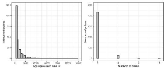
Figure 1: Histogram of the (positive) aggregate claim amount of individual polices (left panel) and bar-plot of the claim numbers for those policies that have one or more claims (right panel) .

5.2 Calculation of the individual risk premium

The first step of the proposed method concerns the estimate of the pure premium. This can be easily performed by a two-part GLMs assuming a binomial distribution with a logistic link function for the claim probability that is corrected for risk exposure, and a Gamma distribution with a log link function for the non-zero claim amount. Table 6 shows the parameter estimates and standard errors for the two-part GLMs with the two most important risk factors, Veh_age and Agecat, and with four and six levels respectively. For the logistic regression part, all the parameters are highly significant (i.e. p-values less than 0.05), except for the first level of Veh_age and the sixth level of Agecat. Although most of risk factor levels are significant in the logistic regression, some of them are not significant in modelling the non-zero claim amount.

The second step concerns the estimate of the risk loading. It can be performed by an expectile regression. Table 7 reports the parameter estimates and standard errors for expectile regression where a 95%-level expectile is considered. While all the levels of Veh_age are not significant in modelling the 95%-level expectile, all the levels of Agecat are highly significant (i.e., p-values less than 0.05), except for the sixth level of Agecat. Figure 2 shows the trend of the parameters in expectile regression over the entire range of expectile levels from 0.05 to 0.95. In each graph, the central continuous line represents the parameter estimates, the external dashed lines represent the upper and lower confidence interval at level 95% estimated by the ER. The linear combination with the intercept parameter allows the estimation of the conditional expectile of the reference tariff: agecat_5 and veg_age_2. In Figure 2, we can observe that intercept and agecat parameters increase as the expectile level increases, while veh_age parameters decrease as the expectile increases. In particular, the veh_age parameters show a slight decrease until 0.75 and a slop afterwards.

Table 6: Parameter estimates of two-part GLMs for modelling claim probability and non-zero claim amount.

Models	Parameters	Estimates	StdError	Z-value	P-value
Logistic regression	(Intercept)	-1.91	0.05	-36.86	0.00
	veh_age_1	-0.03	0.05	-0.62	0.54
	veh_age_3	-0.13	0.04	-2.89	0.00
	veh_age_4	-0.22	0.05	-4.88	0.00
	agecat_1	0.53	0.07	7.80	0.00
	agecat_2	0.33	0.06	5.81	0.00
	agecat_3	0.27	0.06	4.92	0.00
	agecat_4	0.23	0.06	4.15	0.00
	agecat_6	0.00	0.07	-0.04	0.97
GA regression	(Intercept)	7.46	0.08	89.33	0.00
	veh_age_1	-0.14	0.08	-1.90	0.06
	veh_age_3	0.11	0.07	1.53	0.13
	veh_age_4	0.25	0.07	3.30	0.00
	agecat_1	0.57	0.12	4.94	0.00
	agecat_2	0.18	0.09	1.89	0.06
	agecat_3	0.14	0.09	1.53	0.13
	agecat_4	0.09	0.09	0.98	0.33
	agecat_6	0.04	0.11	0.38	0.70

• Notes: The log link function is used in the GA regression model.

Table 7: Parameter estimates of expectile regression model for modelling the aggregate claim amount data ($\tau=0.95$).

Parameters	Estimates	StdError	Z-value	P-value
(Intercept)	1521.26	47.34	32.14	0.00
veh_age_1	-205.14	170.58	-1.20	0.23
veh_age_3	-120.43	129.99	-0.93	0.35
veh_age_4	-72.35	133.56	-0.54	0.59
agecat_1	1260.92	223.62	5.64	0.00
agecat_2	570.65	157.55	3.62	0.00
agecat_3	341.32	123.95	2.75	0.01
agecat_4	337.29	133.25	2.53	0.01
agecat_6	63.69	164.83	0.39	0.70

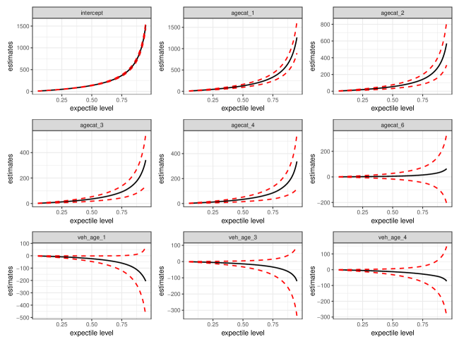
Figure 2: The estimates of parameters in ER model for expectile level varying from $\tau=0.05$ to $\tau=0.95$. The 95% confidence interval are provided by the red dashed curves. .

Table 8 and Table 9 present the risk premiums and the risk loadings for 24 tariff classes predicted using the ER model, along with the GLMs, QR reported in Heras et al. (2018), PQR reported in Baione and Biancalana (2020) and QRII reported in Baione and Biancalana (2019). Five premium principles (i.e., EVPP, SDPP, QPP, TSQPP, EPP) are used to calculate the individual policy risk premiums in existing studies. For ease of comparison with the results of the other studies, we use the same estimation result of quantile regression models (i.e., QR and PQR) as given in Heras et al. (2018) and Baione and Biancalana (2020) when the quantile level $\tau=95\%$ . The same total risk premium of the whole portfolio that the insurer should charge $C=\$22,206,147$ is considered in the following.

For the given $C=\$22,206,147$, it allows us to estimate the risk loading parameter $\varphi$ in the EVPP, SDPP, QPP and EPP using (13). The result of QRII is reported for the risk loading parameter $\tau=79.08\%$ in Baione and Biancalana (2019). We also observe that the risk loading in GLMs is expressed as 11.97% of the pure premium using the EVPP, and 2.31% of the deviation using the SDPP, as well as 3.00% and 3.09% of the distance between VaR and pure premium in QR and PQR using QPP, respectively. Although the PQR describes the regression coefficients’ functional form parametrically depending on the order of the quantile level, QR and PQR yield similar estimates of the risk loading parameter around 3.00%, whereas the estimate of risk loading parameter is 2.85% in the ER model. A possible explanation is that the expectile is considered as the basis of risk loading in EPP, which yields larger prediction than the quantile as it gives more information about both the lower and upper tails of the distribution. From the results we have obtained in Table 8 and Table 9, we conclude:

1. Although two different quantile regressions (i.e. QR and PQR) are employed, the pattern of these two results is similar due to use of the same premium principle.

2. Quantile regressions (i.e. QR and PQR) overestimate the risk loadings for high-risk classes (i.e, class 1, 2 and 3), and underestimate them for low-risk classes (i.e. class 19, 21, 23), while it does not happen in the ER and GLMs.

3. Larger predictions are observed in QRII. Moreover, a negative value of risk loading is also observed in class 20. The presence of negative risk loading might be a drawback when the TSQPP is used for classification ratemaking.

For a graphical comparison that confirms the results in Table 8, we show the predictive risk loading ratios for the 24 tariff classes based on the Figure 3’s competing models. The risk loading ratio is defined as the risk loading divided by the predictive pure premium. The risk loading ratio in GLMs (EVPP) is constant among tariff classes. While it shows the similar pattern in ER and GLMs (SDPP), more variation among tariff classes in ER is observed than in GLMs (SDPP), which indicates the proposed model has the advantage of better differentiating the heterogeneity among tariff classes. QR model has a poor model performance in sense that a opposite trend is observed.

Table 8: Classification risk premiums predicted by different models.

Tariff Class	$\hat{p}_{i}$	Pure premium	ER	GLMs		QR	PQR	QRII
			EPP $\varphi=2.85\%$	EVPP $\varphi=11.97\%$	SDPP $\varphi=2.31\%$	QPP $\varphi=3.00\%$	QPP $\varphi=3.09\%$	TSQPP $\tau=79.08\%$
1-V2A1	0.798	522.88	578.98	585.45	575.97	603.63	602.93	728.58
2-V1A1	0.803	484.58	535.93	542.56	534.43	546.13	550.16	585.84
3-V3A1	0.818	484.98	538.73	543.01	536.93	557.52	562.59	771.13
4-V2A2	0.828	355.42	396.64	397.95	394.69	396.57	396.55	415.44
5-V4A1	0.831	491.20	546.14	549.98	546.00	564.34	570.14	784.62
6-V1A2	0.833	329.07	365.21	368.45	365.94	361.44	362.93	333.73
7-V2A3	0.837	302.31	338.52	338.49	336.62	339.95	339.79	381.75
8-V1A3	0.841	279.83	310.84	313.31	312.03	311.27	310.90	306.58
9-V2A4	0.843	296.12	332.39	331.56	330.36	327.68	329.20	346.93
10-V3A2	0.846	328.44	367.01	367.75	366.80	369.35	367.72	438.08
11-V1A4	0.847	274.05	305.11	306.84	306.18	300.14	301.50	278.58
12-V3A3	0.853	279.08	312.52	312.47	312.57	315.36	314.73	402.14
13-V4A2	0.857	331.81	371.65	371.52	372.21	373.98	371.19	444.62
14-V3A4	0.859	273.17	306.67	305.86	306.58	303.50	304.56	365.21
15-V4A3	0.865	281.74	316.47	315.45	316.99	317.41	317.31	407.84
16-V4A4	0.87	275.65	310.44	308.63	310.80	306.74	306.85	370.22
17-V2A5	0.871	215.94	244.89	241.78	243.59	239.92	238.77	273.48
18-V2A6	0.871	234.28	264.52	262.31	264.32	261.66	259.32	257.69
19-V1A5	0.874	199.67	223.25	223.57	225.60	218.81	219.07	219.41
20-V1A6	0.875	216.63	241.53	242.55	244.80	238.56	238.00	206.73
21-V3A5	0.884	198.53	224.55	222.28	225.45	220.03	219.79	286.91
22-V3A6	0.885	215.38	242.73	241.15	244.62	240.96	239.05	270.33
23-V4A5	0.894	199.86	227.21	223.77	228.15	220.55	220.20	290.16
24-V4A6	0.894	216.82	245.49	242.76	247.55	242.19	239.68	273.39

• Notes: All the results are obtained for one risk exposure (i.e. one policy year). 24 tariff classes have been subdivided according to the two risk factor: Veh_age and Agecat. The symbol V1A1 in Column 1 denotes the policyholder with Veh_age and Agecate both in the level 1. Column 2 reports the predicted probability of incurring no claim. Column 3 reports the predicted pure premium. QR and PQR denote two quantile regressions discussed in Heras et al. (2018) and Baione and Biancalana (2020) respectively. QRII represents the two-stage quantile regression proposed in Baione and Biancalana (2019). ER denotes the expectile regression model. EVPP, SDPP, QPP, EPP, and TSQPP denote various premium principles listed in Table 1.

Table 9: Classification risk loadings predicted by different models.

Tariff Class	$\hat{p}_{i}$	Pure premium	ER	GLMs		QR	PQR	QRII
			EPP $\varphi=2.85\%$	EVPP $\varphi=9.73\%$	SDPP $\varphi=2.31\%$	QPP $\varphi=3.00\%$	QPP $\varphi=3.09\%$	TSQPP $\tau=79.08\%$
1-V2A1	0.798	522.88	56.10	62.57	53.09	80.75	80.05	205.70
2-V1A1	0.803	484.58	51.35	57.99	49.85	61.55	65.58	101.26
3-V3A1	0.818	484.98	53.75	58.03	51.96	72.54	77.61	286.15
4-V2A2	0.828	355.42	41.22	42.53	39.28	41.15	41.13	60.02
5-V4A1	0.831	491.20	54.94	58.78	54.80	73.14	78.95	293.42
6-V1A2	0.833	329.07	36.13	39.38	36.86	32.37	33.86	4.66
7-V2A3	0.837	302.31	36.21	36.18	34.31	37.64	37.48	79.43
8-V1A3	0.841	279.83	31.01	33.49	32.20	31.44	31.07	26.76
9-V2A4	0.843	296.12	36.27	35.43	34.24	31.56	33.08	50.81
10-V3A2	0.846	328.44	38.56	39.30	38.36	40.90	39.27	109.64
11-V1A4	0.847	274.05	31.06	32.79	32.13	26.09	27.45	4.53
12-V3A3	0.853	279.08	33.44	33.40	33.49	36.28	35.65	123.06
13-V4A2	0.857	331.81	39.83	39.71	40.40	42.17	39.37	112.80
14-V3A4	0.859	273.17	33.49	32.69	33.40	30.33	31.39	92.04
15-V4A3	0.865	281.74	34.73	33.71	35.25	35.67	35.57	126.11
16-V4A4	0.870	275.65	34.79	32.98	35.16	31.09	31.21	94.57
17-V2A5	0.871	215.94	28.95	25.84	27.65	23.98	22.83	57.54
18-V2A6	0.871	234.28	30.24	28.03	30.04	27.38	25.05	23.41
19-V1A5	0.874	199.67	23.58	23.89	25.93	19.14	19.40	19.73
20-V1A6	0.875	216.63	24.91	25.92	28.17	21.93	21.38	-9.89
21-V3A5	0.884	198.53	26.02	23.76	26.92	21.50	21.26	88.38
22-V3A6	0.885	215.38	27.35	25.77	29.25	25.58	23.67	54.95
23-V4A5	0.894	199.86	27.35	23.92	28.29	20.69	20.34	90.31
24-V4A6	0.894	216.81	28.68	25.94	30.74	25.38	22.86	56.57

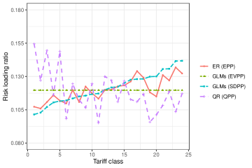
Figure 3: Risk loading ratio estimation based on the ER model, along with the results of existing studies.

5.3 Performance Comparison

For model comparison, the frequently used loss functions, e.g., the root mean square error or mean square error, are not quite informative enough to capture the difference between the predictive values and the corresponding outcomes for individual claim data, due to the high proportions of zeros and the highly right-skewed features. For this reason, we consider the ordered Lorenz curve and the associated Gini index as a statistical measure of the association between the premium and loss distributions in non-life insurance, through which different predictive models can be compared (Frees et al., 2011, Yang et al., 2018, Shi and Yang, 2018).

The ordered Lorenz curve is a plot with the ordered loss distribution on the vertical axis and the ordered premium distribution on the horizontal axis both sorted based on the relative premium (“competing premium”/“base premium” ), where “base premium” is calculated using an existing premium prediction model and “competing premium” is calculated using an alternative premium prediction. The associated Gini index is defined as twice the area between the ordered Lorenz curve and the line of equality. The logic behind this idea is that a score with a greater Gini index produces a greater separation among the observations. In other words, a higher Gini index indicates greater ability to distinguish good risks from bad risks. Following Frees et al. (2011) and Yang et al. (2018), the key to selecting the most favorable model is first to specify the prediction from each model as a base premium and use the prediction from the remaining models as the competing premium.

We calculate the risk premium for each individual policyholder based on GLMs, QR, QRII, PQR and ER models, taking the actual exposure and risk factors of insured $i$ into account . In Table 8, the Gini indices and standard errors are reported by averaging the results from 20 random samples splitting when specifying different combinations of base premium and competing premium. The “mini-max” strategy is usually used to select the “best” model, that is, we first select the model that provides the largest Gini index for each base premium, and then the smallest one taking over competing premiums. We observe that the maximal Gini index is 9.68, 8.33, 11.58, 11.64, and 0 when using the GLMs (i.e., EVPP and SDPP), QR, PQR, ER, and QRII as the base premium. ER with the proposed EPP has the smallest maximum Gini index at 0, hence it is most robust to the alternative model . Figure 4 displays the ordered Lorenz curves of the proposed models. It is obvious that when the ER model is selected as the base premium, the area between the line of equality and the ordered Lorentz curve is smaller than the competing models, indicating that the ER model represents the most favorable choice again.

Table 10: The averaged Gini indices and standard errors in the automobile claim data example based on 20 random splits.

Base premium	Competing premium						Mini-max
	GLMs (EVPP)	GLMs (SDPP)	QR	PQR	ER	QRII
GLMs (EVPP)	0 (0)	8.86 (1.94)	-9.64 (1.90)	-10.06 (1.92)	9.68 (2.04)	-1.95 (1.97)	9.68
GLMs (SDPP)	-7.65 (1.94)	0 (0)	-8.41 (1.91)	-8.51 (1.92)	8.33 (2.08)	-3.41 (1.93)	8.33
QR	11.29 (1.90)	11.25 (1.90)	0 (0)	-0.78 (2.07)	11.58 (1.97)	0.98 (2.06)	11.58
PQR	11.62 (1.92)	11.26 (1.92)	1.1 (2.07)	0 (0)	11.64 (1.98)	1.03 (2.07)	11.64
ER	-6.36 (2.03)	-6.11 (2.07)	-6.65 (1.98)	-6.78 (1.98)	0 (0)	-5.15 (1.91)	0.00
QRII	8.62 (1.97)	10.3 (1.92)	5.66 (2.06)	5.54 (2.07)	12.83 (1.90)	0 (0)	12.83

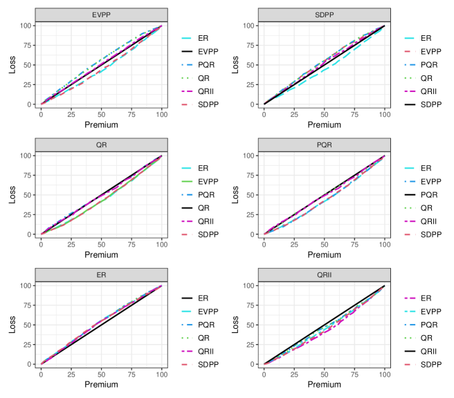
Figure 4: The ordered Lorenz curves for the automobile claim data.

6 Conclusion

In this paper, we propose the expectile regression based on a new Expectile Premium Principle as an important complement to the conventional GLMs as well as quantile regression in the ratemaking mechanism. Our approach has the following advantages: (1) The proposed EPP is a coherent risk measure, thus overcoming the drawbacks of QPP discussed in the recent literature. (2) The risk premium obtained in EPP depends on the shape of the entire distribution and contains more information about both upper and lower tails of distribution. (3) The proposed ratemaking method is computationally efficient. It enables the estimation of the conditional expectile of the aggregate claim amount for all expectile levels in one run, thus allowing us not to lose efficiency in the risk premium estimations. (4) The simulation and empirical result both suggest that expectile regression outperforms the conventional GLMs and quantile regressions, since it can better differentiate the heterogeneity among tariff classes and has a greater ability to distinguish high risks from low risks for the insurers.

It is worth mentioning that the applications of the expectile regressions can go beyond the insurance premium prediction and be of interest to researchers in many other fields including capital allocation, catastrophe risk modelling, and loss reserve assessment in actuarial science. Some extensions of this method with expectile regressions for modelling multivariate loss data could be studied in future research.

Declaration of interest

We declare that there is no potential conflict of interest in the paper.

References

- Artzner et al. (1999) Philippe Artzner, Freddy Delbaen, Jean-Marc Eber, and David Heath. Coherent measures of risk. Mathematical finance, 9(3):203–228, 1999.
- Baione and Biancalana (2019) Fabio Baione and Davide Biancalana. An individual risk model for premium calculation based on quantile: A comparison between generalized linear models and quantile regression. North American Actuarial Journal, 23:1–18, 2019.
- Baione and Biancalana (2020) Fabio Baione and Davide Biancalana. An application of parametric quantile regression to extend the two-stage quantile regression for ratemaking. Scandinavian Actuarial Journal, pages 1–15, 2020.
- Bellini et al. (2014) Fabio Bellini, Bernhard Klar, Alfred Müller, and Emanuela Rosazza Gianin. Generalized quantiles as risk measures. Insurance: Mathematics and Economics, 54:41–48, 2014.
- De Jong et al. (2008) Piet De Jong, Gillian Z Heller, et al. Generalized linear models for insurance data. Cambridge University Press, 2008.
- Dong et al. (2015) Alice XD Dong, Jennifer SK Chan, and Gareth W Peters. Risk margin quantile function via parametric and non-parametric bayesian approaches. ASTIN Bulletin: The Journal of the IAA, 45(3):503–550, 2015.
- Föllmer and Schied (2002) Hans Föllmer and Alexander Schied. Convex measures of risk and trading constraints. Finance and Stochastics, 6(4):429–447, 2002.
- Frees (2009) Edward W Frees. Regression modeling with actuarial and financial applications. Cambridge University Press, 2009.
- Frees et al. (2011) Edward W Frees, Glenn Meyers, and A David Cummings. Summarizing insurance scores using a gini index. Journal of the American Statistical Association, 106(495):1085–1098, 2011.
- Frees et al. (2013) Edward W Frees, Xiaoli Jin, and Xiao Lin. Actuarial applications of multivariate two-part regression models. Annals of Actuarial Science, 7(2):258–287, 2013.
- Frumento and Bottai (2016) Paolo Frumento and Matteo Bottai. Parametric modeling of quantile regression coefficient functions. Biometrics, 72(1):74–84, 2016.
- Frumento and Bottai (2017) Paolo Frumento and Matteo Bottai. An estimating equation for censored and truncated quantile regression. Computational Statistics & Data Analysis, 113:53–63, 2017.
- Gilchrist (2000) Warren Gilchrist. Statistical modelling with quantile functions. Chapman and Hall/CRC, 2000.
- Henckaerts et al. (2018) Roel Henckaerts, Katrien Antonio, Maxime Clijsters, and Roel Verbelen. A data driven binning strategy for the construction of insurance tariff classes. Scandinavian Actuarial Journal, 2018(8):681–705, 2018.
- Heras et al. (2018) Antonio Heras, Ignacio Moreno, and José L Vilar-Zanón. An application of two-stage quantile regression to insurance ratemaking. Scandinavian Actuarial Journal, pages 1–17, 2018.
- Koenker and Bassett Jr (1978) Roger Koenker and Gilbert Bassett Jr. Regression quantiles. Econometrica: Journal of the Econometric Society, pages 33–50, 1978.
- Koenker and Hallock (2001) Roger Koenker and Kevin F Hallock. Quantile regression. Journal of Economic Perspectives, 15(4):143–156, 2001.
- Krämer et al. (2013) Nicole Krämer, Eike C Brechmann, Daniel Silvestrini, and Claudia Czado. Total loss estimation using copula-based regression models. Insurance: Mathematics and Economics, 53(3):829–839, 2013.
- Kuan et al. (2009) Chung-Ming Kuan, Jin-Huei Yeh, and Yu-Chin Hsu. Assessing value at risk with care, the conditional autoregressive expectile models. Journal of Econometrics, 150(2):261–270, 2009.
- Kudryavtsev (2009) Andrey A Kudryavtsev. Using quantile regression for rate-making. Insurance: Mathematics and Economics, 45(2):296–304, 2009.
- Newey and Powell (1987) Whitney K Newey and James L Powell. Asymmetric least squares estimation and testing. Econometrica: Journal of the Econometric Society, pages 819–847, 1987.
- Shi and Yang (2018) Peng Shi and Lu Yang. Pair copula constructions for insurance experience rating. Journal of the American Statistical Association, 113(521):122–133, 2018.
- Smyth and Jørgensen (2002) Gordon K Smyth and Bent Jørgensen. Fitting tweedie’s compound poisson model to insurance claims data: dispersion modelling. ASTIN Bulletin: The Journal of the IAA, 32(1):143–157, 2002.
- Sobotka et al. (2013) Fabian Sobotka, Göran Kauermann, Linda Schulze Waltrup, and Thomas Kneib. On confidence intervals for semiparametric expectile regression. Statistics and Computing, 23(2):135–148, 2013.
- Waltrup et al. (2015) Linda Waltrup, Fabian Otto-Sobotka, Thomas Kneib, and Goeran Kauermann. Expectile and quantile regression–david and goliath? Statistical Modelling, 15:433–456, 10 2015. doi: 10.1177/1471082X14561155.
- Wang (2000) Shaun S Wang. A class of distortion operators for pricing financial and insurance risks. Journal of Risk and Insurance, pages 15–36, 2000.
- Xie et al. (2014) Shangyu Xie, Yong Zhou, and Alan TK Wan. A varying-coefficient expectile model for estimating value at risk. Journal of Business & Economic Statistics, 32(4):576–592, 2014.
- Yang et al. (2018) Yi Yang, Wei Qian, and Hui Zou. Insurance premium prediction via gradient tree-boosted tweedie compound poisson models. Journal of Business & Economic Statistics, 36(3):456–470, 2018.
- Yao and Tong (1996) Qiwli Yao and Howell Tong. Asymmetric least squares regression estimation: a nonparametric approach. Journal of Nonparametric Statistics, 6(2-3):273–292, 1996.