PMC_∞: Infinite-Order Scale-Setting using the Principle of Maximum Conformality A Remarkably Efficient Method for Eliminating Renormalization Scale Ambiguities for Perturbative QCD

Abstract

We identify a property of renormalizable SU(N)/U(1) gauge theories, the Intrinsic Conformality ($iCF$), which underlies the scale invariance of physical observables and leads to a remarkably efficient method to solve the conventional renormalization scale ambiguity at every order in pQCD: the PMC_∞. This new method reflects the underlying conformal properties displayed by pQCD at NNLO, eliminates the scheme dependence of pQCD predictions and is consistent with the general properties of the PMC (Principle of Maximum Conformality). We introduce a new method to identify conformal and $\beta$-terms which can be applied either to numerical or to theoretical calculations. We illustrate the PMC_∞ for the thrust and C-parameter distributions in $e^{+}e^{-}$ annihilation and then we show how to apply this new method to general observables in QCD. We point out how the implementation of the PMC_∞ can significantly improve the precision of pQCD predictions; its implementation in multi-loop analysis also simplifies the calculation of higher orders corrections in a general renormalizable gauge theory.

.1 Introduction

A key issue in making precise predictions in QCD is the uncertainty in setting the renormalization scale $\mu_{R}$ in order to determine the correct running coupling $\alpha_{s}(\mu_{R}^{2})$ in the perturbative expansion of a scale invariant quantity. The Conventional practice of simply guessing the scale $\mu_{R}$ of the order of a typical momentum transfer Q in the process, and then varying the scale over a range Q/2 and 2Q, gives predictions which depend on the renormalization scheme, retains dependence on the initial scale choice, leads to a non-conformal series which diverges as $\sim\alpha_{s}^{n}\beta_{0}^{n}n!$, and is even invalid for QEDmaitre:2009xp . In fact, a physical process will depend on many invariants and thus have multiple renormalization scales which depend on the dynamics of the process. Other proposals for renormalization scale setting such as PMS stevenson or FAC grunberg not only have the same difficulties, but they also lead to incorrect and unphysical results kramer . It has been shown recently how all the theoretical constraints can be satisfied at once, leading to accurate results by using the PMC (the Principle of Maximum Conformality) PMC1 ; PMC2 ; PMC3 . The primary purpose of the PMC method is to solve the scale-setting ambiguity, it has been extended to all orders mojaza1 ; mojaza2 and it determines the correct running coupling and the correct momentum flow accordingly to the RGE invariance xing1 ; xing2 . This leads to results that are invariant respect to the initial renormalization scale in agreement with the requirement of scale invariance of an observable in pQCD xing3 .
We show here, how the implementation at all orders of the PMC simplifies in many cases by identifying only the $\beta_{0}$-terms at each order of accuracy due to the presence of a new property of the perturbative corrections. First we recall that there is no ambiguity in setting the renormalization scale in QED. The standard Gell-Mann-Low scheme determines the correct renormalization scale identifying the scale with the virtuality of the exchanged photon qed . For example, in electron-muon elastic scattering, the renormalization scale is the virtuality of the exchanged photon, i.e. the spacelike momentum transfer squared $\mu_{R}^{2}=q^{2}=t$. Thus

$$\alpha(t)={\alpha(t_{0})\over 1-\Pi(t,t_{0})}$$ (1)

where

$$\Pi(t,t_{0})={\Pi(t)-\Pi(t_{0})\over 1-\Pi(t_{0})}$$

From Eq.1 it follows that the renormalization scale $\mu_{R}=t$ can be determined by the $\beta_{0}$-term at the lowest order. This scale is sufficient to sum all the vacuum polarization contributions into the dressed photon propagator, both proper and improper at all orders. Again in QED, considering the case of two photon exchange a new different scale is introduced in order to absorb all the $\beta$-terms related to the new subset/subprocess into the scale. Also in this case the scale can be determined by identifying the lowest order $\beta_{0}$-term alone. This term identifies the virtuality of the exchanged momenta causing the running of the scale in that subprocess. This scale again would sum all the contributions related to the $\beta$-function into the renormalization scale and no further corrections need to be introduced to the scale at higher orders. Given that the pQCD and pQED predictions match analytically in the $N_{C}\to 0$ limit where $C_{F}\alpha_{QCD}\to\alpha_{QED}$ (see ref. huet ) we extend the same procedure to pQCD. In fact in many cases in QCD the $\beta_{0}$ terms alone can determine the pQCD renormalization scale at all orders padeapp eliminating the renormalon contributions $\alpha_{s}^{n}\beta_{0}^{n}n!$. Though in non-Abelian theories other diagrams related to the three- and four-gluon vertices arise, these terms do not necessarily spoil this procedure. In fact, in QCD, the $\beta_{0}$ terms arising from the renormalization of the three-gluon or four-gluon vertices as well as from gluon wavefunction renormalization determine the renormalization scales of the respective diagrams and no further corrections to the scales need to be introduced at higher orders. In conclusion, if we focus on a particular class of diagrams we can fix the PMC scale by determining the $\beta_{0}$-term alone and we show this to be connected to the general scale invariance of an observable in a gauge theory. We introduce in this article a parametrization of the observables which stems directly from the analysis of the perturbative QCD corrections and which reveals interesting properties like scale invariance independently from the process or from the kinematics. We point out that this parametrization can be an intrinsic general property of gauge theories and we define this property as Intrinsic Conformality (iCF). We also show how this property directly indicates what is the correct renormalization scale $\mu_{R}$ at each order of calculation and we define this new method PMC_∞:Infinite-Order Scale-Setting using the Principle of Maximum Conformality. We discuss the iCF property and the PMC_∞ for the case of the thrust and C-parameter distributions in $e^{+}e^{-}\rightarrow 3jets$ and we show the results.

In general a normalized IR safe single variable observable, such as the thrust distribution for the $e^{+}e^{-}\rightarrow 3jets$ thrust1 ; thrust2 , is the sum of pQCD contributions calculated up to NNLO at the initial renormalization scale $\mu_{0}$:

$$\frac{1}{\sigma_{0}}\!\frac{Od\sigma(\mu_{0})}{dO}\! \!\!=\!\! \!\left\{\!\frac{\alpha_{s}(\mu_{0})}{2\pi}\!\frac{OdA_{\mathit{O}}(\mu_{0})}{dO}\!+\!\!\left(\!\frac{\alpha_{s}(\mu_{0})}{2\pi}\!\right)^{\!\!2}\!\!\frac{OdB_{\mathit{O}}(\mu_{0})}{dO}\right.$$ (2)

$$+\left.\left(\frac{\alpha_{s}(\mu_{0})}{2\pi}\right)^{\!\!3}\!\frac{OdC_{\mathit{O}}(\mu_{0})}{dO}\!+\!{\cal O}(\alpha_{s}^{4})\right\},$$

where the $\sigma_{0}$ is tree-level hadronic cross section, the $A_{O},B_{O},C_{O}$ are respectively the LO, NLO and NNLO coefficients, $O$ is the selected non-integrated variable. For sake of simplicity we will refer to the differential coefficients as to implicit coefficients and we drop the derivative symbol, i.e.

$$A_{O}(\mu_{0})~{}\!\! \equiv ~{}~{}\frac{OdA_{O}(\mu_{0})}{dO},\,B_{O}(\mu_{0})~{}\equiv~{}~{}\frac{OdB_{O}(\mu_{0})}{dO},$$

$$C_{O}(\mu_{0})~{}\!\! \equiv ~{}\frac{OdC_{O}(\mu_{0})}{dO}.$$ (3)

We define here the Intrinsic Conformality as the property of a renormalizable SU(N)/U(1) gauge theory, like QCD, which yields to a particular structure of the perturbative corrections that can be made explicit representing the perturbative coefficients using the following parametrization:

$$A_{O}(\mu_{0})\!\!\! = \!\!\!A_{\mathit{Conf}},$$

$$B_{O}(\mu_{0})\!\!\! = \!\!\!B_{\mathit{Conf}}+\frac{1}{2}\beta_{0}\ln\left(\frac{\mu_{0}^{2}}{\mu_{I}^{2}}\right)A_{\mathit{Conf}},$$

$$C_{O}(\mu_{0})\!\!\! = \!\!\!C_{\mathit{Conf}}+\beta_{0}\ln\left(\frac{\mu_{0}^{2}}{\mu_{II}^{2}}\right)B_{\mathit{Conf}}+$$

$$\!\!\!+\frac{1}{4}\left[\beta_{1}+\beta_{0}^{2}\ln\left(\frac{\mu_{0}^{2}}{\mu_{I}^{2}}\right)\right]\ln\left(\frac{\mu_{0}^{2}}{\mu_{I}^{2}}\right)A_{\mathit{Conf}}$$

where the $A_{\mathit{Conf}},B_{\mathit{Conf}},C_{\mathit{Conf}}$ are the scale invariant Conformal Coefficients (i.e. the coefficients of each perturbative order not depending on the scale $\mu_{0}$) while we define the $\mu_{N}$ as Intrinsic Conformal Scales and $\beta_{0},\beta_{1}$ are the first two coefficients of the $\beta$-function. We remind that the implicit coefficients are defined at the scale $\mu_{0}$ and that they change according to the standard RG equations under a change of the renormalization scale according to :

$$A_{O}(\mu_{R})\!\!\! = \!\!\!A_{O}(\mu_{0}),$$

$$B_{O}(\mu_{R})\!\!\! = \!\!\!B_{O}(\mu_{0})+\frac{1}{2}\beta_{0}\ln\left(\frac{\mu_{R}^{2}}{\mu_{0}^{2}}\right)A_{O}(\mu_{0}),$$

$$C_{O}(\mu_{R})\!\!\! = \!\!\!C_{O}(\mu_{0})+\beta_{0}\ln\left(\frac{\mu_{R}^{2}}{\mu_{0}^{2}}\right)B_{O}(\mu_{0})+$$

$$\!\!\!+\frac{1}{4}\left[\beta_{1}+\beta_{0}^{2}\ln\left(\frac{\mu_{R}^{2}}{\mu_{0}^{2}}\right)\right]\ln\left(\frac{\mu_{R}^{2}}{\mu_{0}^{2}}\right)A_{O}(\mu_{0})$$

It can be shown that the form of Eq.LABEL:newevolution is scale invariant and it is preserved under a change of the renormalization scale from $\mu_{0}$ to $\mu_{R}$ by standard RG equations Eq.LABEL:standardevolution, i.e.:

$$A_{O}(\mu_{R})\!\!\! = \!\!\!A_{\mathit{Conf}},$$

$$B_{O}(\mu_{R})\!\!\! = \!\!\!B_{\mathit{Conf}}+\frac{1}{2}\beta_{0}\ln\left(\frac{\mu_{R}^{2}}{\mu_{I}^{2}}\right)A_{\mathit{Conf}},$$

$$C_{O}(\mu_{R})\!\!\! = \!\!\!C_{\mathit{Conf}}+\beta_{0}\ln\left(\frac{\mu_{R}^{2}}{\mu_{II}^{2}}\right)B_{\mathit{Conf}}+$$ (6)

$$\!\!\!+\frac{1}{4}\left[\beta_{1}+\beta_{0}^{2}\ln\left(\frac{\mu_{R}^{2}}{\mu_{I}^{2}}\right)\right]\ln\left(\frac{\mu_{R}^{2}}{\mu_{I}^{2}}\right)A_{\mathit{Conf}}$$

We notice that the form of Eq. LABEL:newevolution is invariant and that the initial scale dependence is exactly removed by $\mu_{R}$. Extending this parametrization to all orders we achieve a scale invariant quantity: the iCF-parametrization is a sufficient condition in order to obtain a scale invariant observable.

In order to show this property we collect together the terms identified by the same conformal coefficient, we name each set as conformal subset and we extend the property to the order $n$:

$$\sigma_{I} \!\!=\!\!\left\{\left(\frac{\alpha_{s}(\mu_{0})}{2\pi}\right)+\frac{1}{2}\beta_{0}\ln\left(\frac{\mu_{0}^{2}}{\mu_{I}^{2}}\right)\left(\frac{\alpha_{s}(\mu_{0})}{2\pi}\right)^{2}\right.$$ (7)

$$\!\!\!\!\!+\!\!\!\!\! \!\!\!\left.\!\!\!\!\frac{1}{4}\!\left[\beta_{1}\!+\!\beta_{0}^{2}\ln\left(\frac{\mu_{0}^{2}}{\mu_{I}^{2}}\right)\right]\ln\left(\frac{\mu_{0}^{2}}{\mu_{I}^{2}}\right)\!\!\left(\frac{\alpha_{s}(\mu_{0})}{2\pi}\right)^{3}\!\!\!+\ldots\!\!\right\}\!\!A_{\mathit{Conf}}$$

$$\sigma_{II} \!\!=\!\!\left\{\left(\frac{\alpha_{s}(\mu_{0})}{2\pi}\right)^{2}\!\!\!\!+\!\beta_{0}\ln\!\left(\!\frac{\mu_{0}^{2}}{\mu_{II}^{2}}\right)\!\!\left(\frac{\alpha_{s}(\mu_{0})}{2\pi}\right)^{3}\!\!\!+\ldots\!\!\right\}\!B_{\mathit{Conf}}$$

$$\sigma_{III} \!\!=\!\!\left\{\left(\frac{\alpha_{s}(\mu_{0})}{2\pi}\right)^{3}+\ldots\right\}C_{\mathit{Conf}},$$

$$\vdots \qquad\qquad.^{.^{.}}$$

$$\sigma_{n} \!\!=\!\!\left\{\left(\frac{\alpha_{s}(\mu_{0})}{2\pi}\right)^{n}\right\}\mathcal{L}_{n\mathit{Conf}},$$

in each subset we have only one intrinsic scale and only one conformal coefficient and the subsets are disjoint, then no mixing terms among the scales or the coefficients are introduced in this parametrization. Besides the structure of the subsets remains invariant under a global change of the renormalization scale as shown from Eq.6. The structure of each conformal set $\sigma_{I},\sigma_{II},\sigma_{III},...$ and consequently the iCF are preserved also if we fix a different renormalization scale for each conformal subset, i.e.:

$$\left(\mu^{2}\frac{\partial}{\partial\mu^{2}}+\beta(\alpha_{s})\frac{\partial}{\partial\alpha_{s}}\right)\sigma_{n}=0.$$ (8)

We define here this property of Eq. 7 of separating an observable in the union of ordered scale invariant disjoint subsets $\sigma_{I},\sigma_{II},\sigma_{III},...$ as ordered scale invariance.

In order to extend the iCF to all orders we first define a partial limit $J_{/n}\rightarrow\infty$ as the limit obtained including the higher order corrections relative only to those $\beta_{0},\beta_{1},\beta_{2},...,\beta_{n-2}$ terms that have been determined already at the order $n$ for each subset and then we perform the complementary $\bar{n}$ limit which consists in including all the remaining terms. For the $J_{/n}$ limit we have:

$$\lim_{J_{/n}\rightarrow\infty} \sigma_{I} \rightarrow\left(\frac{\left.\alpha_{s}(\mu_{I})\right|_{n-2}}{2\pi}\right)A_{\mathit{Conf}}$$

$$\lim_{J_{/n}\rightarrow\infty} \sigma_{II} \rightarrow\left(\frac{\left.\alpha_{s}(\mu_{II})\right|_{n-3}}{2\pi}\right)^{2}B_{\mathit{Conf}}$$

$$\lim_{J_{/n}\rightarrow\infty} \sigma_{III} \rightarrow\left(\frac{\left.\alpha_{s}(\mu_{\mathit{III}})\right|_{n-4}}{2\pi}\right)^{3}C_{\mathit{Conf}}$$

$$\vdots \qquad\qquad\vdots$$

$$\lim_{J_{/n}\rightarrow\infty} \sigma_{n} \equiv\left(\frac{\alpha_{s}(\mu_{0})}{2\pi}\right)^{n}\mathcal{L}_{n\mathit{Conf}}$$ (9)

where the $\left.\alpha_{s}(\mu_{I})\right|_{n-2}$ is the coupling calculated up to the $\beta_{n-2}$ at the intrinsic scale $\mu_{I}$. Given the particular ordering of the powers of the coupling, in each conformal subset we have the coefficients of the $\beta_{0},...,\beta_{n-k-1}$ terms, where $k$ is the order of the conformal subset and the $n$ is the order of the highest subset with no $\beta$-terms. We notice that the limit of each conformal subset is finite and scale invariant up to the $\sigma_{n-1}$. The remaining scale dependence is confined in the coupling of the $n^{th}$ term. Any combination of the $\sigma_{I},...,\sigma_{n-1}$ subsets is finite and scale invariant. We can now extend the iCF to all orders performing the $\bar{n}$ limit. In this limit we include all the remaining higher order corrections. For the calculated conformal subsets this leads to define the coupling at the same scales but including all the missing $\beta$ terms. Thus each conformal subset remains scale invariant. We point out that we are not making any assumption on the convergence of the series for this limit. Then we have:

$$\lim_{\bar{n}\rightarrow\infty} \sigma_{I} \rightarrow\left(\frac{\alpha_{s}(\mu_{I})}{2\pi}\right)A_{\mathit{Conf}}$$

$$\lim_{\bar{n}\rightarrow\infty} \sigma_{II} \rightarrow\left(\frac{\alpha_{s}(\mu_{II})}{2\pi}\right)^{2}B_{\mathit{Conf}}$$

$$\lim_{\bar{n}\rightarrow\infty} \sigma_{III} \rightarrow\left(\frac{\alpha_{s}(\mu_{\mathit{III}})}{2\pi}\right)^{3}C_{\mathit{Conf}}$$

$$\vdots \qquad\qquad\vdots$$

$$\lim_{\bar{n}\rightarrow\infty} \sigma_{n}\!\! \!\!\equiv\!\!\lim_{n\rightarrow\infty}\left(\frac{\alpha_{s}(\mu_{0})}{2\pi}\right)^{n}\!\!\mathcal{L}_{n\mathit{Conf}}\!\!\rightarrow\hbox{Conformal Limit}$$

where here now $\alpha_{s}(\mu_{I})$ is the complete coupling determined at the same scale $\mu_{I}$. The Eq.LABEL:nlimit shows that the whole renormalization scale dependence has been completely removed. In fact both the intrinsic scales $\mu_{N}$ and the conformal coefficients $A_{\mathit{Conf}},B_{\mathit{Conf}},C_{\mathit{Conf}},...,\mathcal{L}_{n\mathit{Conf}},...$ are not depending on the particular choice of the initial scale. The only term with a residual $\mu_{0}$ dependence is the n-term, but this dependence cancels in the limit $n\rightarrow\infty$. The scale dependence is totally confined in the coupling $\alpha_{s}(\mu_{0})$ and its behavior doesn’t depend on the particular choice of any scale $\mu_{0}$ in the perturbative region, i.e. $\lim_{n\rightarrow\infty}\alpha_{s}(\mu_{0})^{n}\sim a^{n}$ with $a<1$. Hence the limit of $\lim_{n\rightarrow\infty}\sigma_{n}$ depends only on the properties of the theory and not on the scale of the coupling in the perturbative regime. The proof given here shows that the iCF is sufficient to have a scale invariant observable and it is not depending on the particular convergence of the series. In order to show the necessary condition we separate the two cases of a convergent series and an asymptotic expansion. For the first case the necessary condition stems directly from the uniqueness of the iCF form, since given a finite limit and the scale invariance any other parametrization can be reduced to the iCF by means of appropriate transformations in agreement with the RG equations. For the second case, we have that an asymptotic expansion though not convergent, can be truncated at a certain order $n$, which is the case of Eq.7. Given the particular structure of the iCF we can perform the first partial limit $J_{/n}$ and we would achieve a finite and scale invariant prediction , $\sigma_{N-1}=\Sigma_{i=1}^{n-1}\sigma_{i}$, for a truncated asymptotic expansion, as shown in Eq. 9. Given the truncation of the series in the region of maximum of convergence the n-th term would be reduced to lowest value and so the scale dependence of the observable would reach its minimum. Given the finite and scale invariant limit $\sigma_{N-1}$ we conclude that the iCF is unique and then necessary for an ordered scale invariant truncated asymptotic expansion up to the $n^{th}$ order. We point out that in general the iCF form is the most general and irreducible parametrization which leads to the scale invariance, other parametrization are forbidden since if we introduce more scales in the logarithms of one subset we would spoil the invariance under the RG transformation and we could not achieve Eq. 6, while on the other hand no scale dependence can be introduced in the intrinsic scales since it would remain in the observable already in the first partial limit $J_{/n}$ and it could not be eliminated. The conformal coefficients are conformal by definition at each order, thus they don’t depend on the renormalization scale and they don’t have a perturbative expansion. Hence the iCF is a necessary and sufficient condition for scale invariance.

.2 The iCF and the ordered scale invariance

The iCF-parametrization can stem either from an inner property of the theory, the iCF, or from direct parametrization of the scale-invariant observable. In both cases the iCF-parametrization makes the scale dependence of the observable explicit and it exactly preserves the scale invariance. Once we have defined an observable in the iCF-form, we have not only the scale invariance of the entire observable, but also the ordered scale invariance (i.e. the scale invariance of each subset $\sigma_{n}$ or $\sigma_{N-1}$). The latter property is crucial in order to obtain scale invariant observables independently from the particular kinematical region and independently from the starting order of the observable or the order of the truncation of the series. Since in general, a theory is blind respect to the particular observable/process that we are going to investigate, the theory should preserve the ordered scale invariance in order to define always scale invariant observables. Hence if the iCF is an inner property of the theory, it leads to implicit coefficients that are neither independent nor conformal. This is made explicit in the Eq.LABEL:newevolution, but it is hidden in the perturbative calculations in case of the implicit coefficients. For instance the presence of the iCF clearly reveals when a particular kinematical region is approached and the $A_{O}$ becomes null. This would cause a break of the scale invariance since a residual initial scale dependence would remain in the observable in the higher orders coefficients. The presence of the iCF solves this issue by leading to the correct redefinition of all the coefficients at each order preserving the correct scale invariance exactly. Thus in the case of a scale invariant observable $O$ defined, according to the implicit form (Eq.2), by the coefficients $\{A_{O},B_{O},C_{O},..,O_{O},...\}$ , it cannot simply undergo the change $\rightarrow\{0,B_{O},C_{O},..,O_{O},...\}$ , since this would break the scale invariance. In order to preserve the scale invariance we must redefine the coefficients $\{\tilde{A}_{O}=0,\tilde{B}_{O},\tilde{C}_{O},..,\tilde{O}_{O},...\}$ cancelling out all the initial scale dependence originated from the LO coefficient $A_{O}$ at all orders. This is equivalent to subtract out a whole invariant conformal subset $\sigma_{I}$ related to the coefficient $A_{\mathit{Conf}}$ from the scale invariant observable $O$. This mechanism is clear in the case of the explicit form of the iCF, Eq. LABEL:newevolution, where if $A_{\mathit{Conf}}=0$ then the whole conformal subset is null and the scale invariance is preserved. We underline that the conformal coefficients can acquire all the possible values without breaking the scale invariance, they contain the essential information on the physics of the process, while all the correlation factors can be reabsorbed in the renormalization scales as shown by the PMC method PMC1 ; PMC2 ; PMC3 ; mojaza1 ; mojaza2 . Hence if a theory has the property of the ordered scale invariance it preserves exactly the scale invariance of observables independently from the process, the kinematics and the starting order of the observable. We put forward that if a theory has the Intrinsic Conformality all the renormalized quantities, such as cross sections, can be parametrized with the iCF-form. This property should be preserved by the renormalization scheme or by the definition of IR safe quantities and it should be preserved also in observables defined in effective theories.

.3 The PMC_∞

We introduce here a new method to eliminate the scale-setting ambiguity in single variable scale invariant distributions named PMC_∞. This method is based on the original PMC principle  PMC1 ; PMC2 ; PMC3 ; mojaza1 ; mojaza2 and agrees with all the PMC different formulations for the PMC-scales at the lowest order. Essentially the core of the PMC_∞ is the same of all the BLM-PMC prescriptionsblm , i.e. the correct running coupling value and hence its renormalization scale at the lowest order is identified by the $\beta_{0}$-term at each order, or equivalently by the intrinsic conformal scale $\mu_{N}$. The PMC_∞ preserves the iCF and then the scale invariance absorbing an infinite set of $\beta$-terms at all orders. This method differs from the other PMC prescriptions since, due to the presence of the Intrinsic Conformality, no perturbative correction in $\alpha_{s}$ needs to be introduced at higher orders in the PMC-scales. Given that all the $\beta$-terms of a single conformal subset are included in the renormalization scale already with the definition at lowest order, no initial scale or scheme dependence are left due to the unknown $\beta$-terms in each subset. The PMC_∞-scale of each subset can be unambiguously determined by $\beta_{0}$-term of each order, we underline that all logarithms of each subset have the same argument and all the differences arising at higher orders have to be included only in the conformal coefficients. Reabsorbing all the $\beta$-terms into the scale also the $\beta_{0}^{n}n!$ terms (related to the renormalons renormalons1 ) are eliminated, thus the precision is improved and the perturbative QCD predictions can be extended to a wider range of values. The initial scale dependence is totally confined in the unknown PMC_∞ scale of the last order of accuracy (i.e. up to NNLO case in the $\alpha_{s}(\mu_{0})^{3}$). Thus if we fix the renormalization scale independently to the proper intrinsic scale for each subset $\mu_{N}$, we end up with a perturbative sum of totally conformal contributions up to the order of accuracy:

$$\!\!\!\!\!\!\!\!\frac{1}{\sigma_{0}}\frac{Od\sigma(\mu_{I},\mu_{II},\mu_{III})}{dO}\!\!\! = \left\{\frac{\alpha_{s}(\mu_{I})}{2\pi}\frac{OdA_{\mathit{Conf}}}{dO}+\!\!\right.$$

$$\!\!\!\!\left(\frac{\alpha_{s}(\mu_{II})}{2\pi}\right)^{2}\!\!\frac{OdB_{\mathit{Conf}}}{dO}\!\! + \!\!\left.\left(\frac{\alpha_{s}(\mu_{III})}{2\pi}\right)^{3}\!\!\frac{OdC_{\mathit{Conf}}}{dO}\right\}$$ (11)

$$\qquad\qquad\qquad\,+{\cal O}(\alpha_{s}^{4}),$$

at this order $\mu_{III}=\mu_{0}$.

.4 iCF coefficients and scales

We describe here how all the coefficients of Eq. LABEL:newevolution can be identified from a numerical either theoretical perturbative calculation. We will use as template the NNLO thrust distribution results calculated in Refs. weinzierl1 ; weinzierl2 . Since the leading order is already ($A_{\mathit{Conf}}$) void of $\beta$-terms we start with NLO coefficients. A general numerical/theoretical calculation keeps tracks of all the color factors and the respective coefficients:

$$B_{O}(N_{f})=C_{F}\left[C_{A}B_{O}^{N_{c}}+C_{F}B_{O}^{C_{F}}+T_{F}N_{f}B_{O}^{N_{f}}\right]$$ (12)

where $C_{F}=\frac{\left(N_{c}^{2}-1\right)}{2N_{c}}$, $C_{A}=N_{c}$ and $T_{F}=1/2.$ The dependence on $N_{f}$ is made explicit here for sake of clarity. We can determine the conformal coefficient $B_{\mathit{Conf}}$ of the NLO order straightforwardly, by fixing the number of flavors $N_{f}$ in order to kill the $\beta_{0}$ term:

$$B_{\mathit{Conf}} = B_{O}\left(N_{f}\equiv\frac{33}{2}\right),$$

$$B_{\beta_{0}}\equiv\log\frac{\mu_{0}^{2}}{\mu_{I}^{2}} = 2\frac{B_{O}-B_{\mathit{Conf}}}{\beta_{0}A_{\mathit{Conf}}}$$ (13)

we would achieve the same results in the usual PMC way, i.e. identifying the $N_{f}$ coefficient with the $\beta_{0}$ term and then determining the conformal coefficient. Both methods are consistent and results for the intrinsic scales and the coefficients are in perfect agreement. At the NNLO a general coefficient is made of the contribution of six different color factors:

$$C_{O}(N_{f}) = \frac{C_{F}}{4}\left\{N_{c}^{2}C_{O}^{N_{c}^{2}}+C_{O}^{N_{c}^{0}}+\frac{1}{N_{c}^{2}}C_{O}^{\frac{1}{N_{c}^{2}}}\right.$$ (14)

$$\!\!\!\!\!\!\!\!\!\!\!\!\!\!\!\!\!\!\!\!\left.\!\!\!\!\!+N_{f}N_{c}\cdot C_{O}^{N_{f}N_{c}}+\frac{N_{f}}{N_{c}}C_{O}^{N_{f}/N_{c}}+N_{f}^{2}C_{O}^{N_{f}^{2}}\right\}.$$

In order to identify all the terms of Eq.LABEL:newevolution we notice first that the coefficients of the terms $\beta_{0}^{2}$ and $\beta_{1}$ are already given by the NLO coefficient $B_{\beta_{0}}$, then we need to determine only the $\beta_{0}$- and the conformal $C_{\mathit{Conf}}$-terms. In order to determine the latter coefficients we use the same procedure we used for the NLO , i.e. we set the number of flavors $N_{f}\equiv 33/2$ in order to drop off all the $\beta_{0}$ terms. We have then:

$$C_{\mathit{Conf}} = C_{O}\left(N_{f}\equiv\frac{33}{2}\right)-\frac{1}{4}\overline{\beta}_{1}B_{\beta_{0}}A_{\mathit{Conf}},$$

$$C_{\beta_{0}}\equiv\log\left(\frac{\mu_{0}^{2}}{\mu_{II}^{2}}\right) = \frac{1}{\beta_{0}B_{\mathit{Conf}}}{\bigg{(}}C_{O}-C_{\mathit{Conf}}$$

$$\!\!\!\!-\left.\frac{1}{4}\beta_{0}^{2}B_{\beta_{0}}^{2}A_{\mathit{Conf}}-\frac{1}{4}\beta_{1}B_{\beta_{0}}A_{\mathit{Conf}}\!\right)\!\!,$$

with $\overline{\beta}_{1}\equiv\beta_{1}(N_{f}=33/2)=-107$. This procedure can be extended at every order and one may decide whether to cancel the $\beta_{0}$, $\beta_{1}$ or $\beta_{2}$ by fixing the appropriate number of flavors. The results can be compared leading to determine exactly all the coefficients. We point out that extending the Intrinsic Conformality to all orders we can predict at this stage the coefficients of all the color factors of the higher orders related to the $\beta$-terms except those related to the higher order conformal coefficients and $\beta_{0}$-terms (e.g. at NNNLO the $D_{\mathit{Conf}}$ and $D_{\beta_{0}}$). The $\beta$-terms are coefficients that stem from UV-divergent diagrams connected with the running of the coupling constant and not from UV-finite diagrams. UV-finite $N_{F}$ terms may arise but would not contribute to the $\beta$-terms. While $N_{f}$ terms coming from UV-divergent diagrams, depending dynamically on the virtuality of the underlying quark and gluon subprocesses have to be considered as $\beta$-terms and they would determine the intrinsic conformal scales. In general, each $\mu_{N}$ is an independent function of the $\sqrt{s}$, of the selected variable $O$ and it varies with the number of colors $N_{c}$ mainly due to $ggg$- and $gggg$-vertices. The latter terms arise at higher orders only in non-Abelian theory but they do not spoil the iCF-form. We underline that iCF applies to scale invariant single variable distributions, in case one is interested in the renormalization of a particular diagram, e.g. the $ggg$-vertex, contributions from different $\beta$-terms should be singled out in order to identify the respective intrinsic conformal scale consistently with the renormalization of the non-Abelian $ggg$-vertex, as shown in binger .

.5 The PMC_∞ scales at LO and NLO

According to the PMC_∞ prescription we fix the renormalization scale to $\mu_{N}$ at each order absorbing all the $\beta$ terms into the coupling. We notice a small mismatch between the zeroes of the conformal coefficient $B_{\mathit{Conf}}$ and those of the remainder $\beta_{0}$-term at the numerator (formula is shown in Eq. LABEL:Cconf). Due to our limited knowledge of the strong coupling at low energies, in order to avoid singularities in the NLO-scale $\mu_{II}$, we introduce a regularization which leads to a finite scale $\tilde{\mu}_{II}$. These singularities stem from a rather logarithmic behavior of the conformal coefficients when low values of the variable $1-T$ are approached. Large logarithms arise from the IR divergences cancellation procedure and they can be resummed in order to restore a predictive perturbative regimeresummation0 ; resummation1 ; resummation2 ; resummation3 ; resummation5 ; resummation6 . We point out that IR cancellation should not spoil the iCF property and a IR cancellation Monte Carlo technique consistent with the iCF would be required. Whether this is an actual deviation from the iCF-form has to be further investigated. However since the discrepancies between the coefficients are rather small, we introduce a regularization method based on redefinition of the norm of the coefficient $B_{\mathit{Conf}}$ in order to cancel out these singularities in the $\mu_{II}$-scale. This regularization is consistent with the PMC principle and up to the accuracy of the calculation it does not introduce any bias effect in the results and no ambiguity in the NLO-PMC_∞ scale. All the differences introduced by the regularization would start at the NNNLO order of accuracy and they can be absorbed after in the higher order PMC_∞ scales. Thus the first two PMC_∞ scales result:

$$\large{\mu}_{\mathit{I}} = \sqrt{s}\cdot e^{-\frac{1}{2}B_{\beta_{0}}},\hskip 54.06006pt{\scriptstyle(1-T)<0.33}$$ (16)

$$\large{\tilde{\mu}}_{\mathit{II}} = \left\{\begin{array}[]{lr}\sqrt{s}\cdot e^{-\frac{1}{2}C_{\beta_{0}}\cdot\frac{B_{\mathit{Conf}}}{B_{\mathit{Conf}}+\eta\cdot A_{\mathit{tot}}A_{\mathit{Conf}}}},\\ \hskip 99.58464pt{\scriptstyle(1-T)<0.33}\\ \sqrt{s}\cdot e^{-\frac{1}{2}\left(\frac{C_{1}}{11B_{1}-\frac{2}{3}B_{0}}\right)},\\ \hskip 99.58464pt{\scriptstyle(1-T)>0.33}\\ \end{array}\right.$$ (21)

where $\sqrt{s}=M_{Z_{0}}$, and the value of $\eta=3.51$ has been fixed by matching the zeroes of numerator and denominator of $C_{\beta_{0}}$. We have to point out that in the region $(1-T)>0.33$ we have a clear example of Intrinsic Conformality-iCF where the kinematical constraints set the $A_{\mathit{Conf}}=0$. According to the Eq.6 setting the $A_{\mathit{Conf}}=0$ the whole conformal subset $\sigma_{I}$ becomes null. In this case all the $\beta$ terms at NLO and NNLO disappear except the $\beta_{0}$-term at NNLO which determines the $\mu_{II}$ scale. The surviving $N_{f}$ terms at NLO or the $N_{f}^{2}$ at NNLO are related to the finite $N_{F}$-term at NLO and to the mixed $N_{f}\cdot N_{F}$ term arising from $B_{O}\cdot\beta_{0}$ at NNLO. Using the following parametrization:

$$A_{O} = 0,$$

$$B_{O} = B_{0}+B_{1}\cdot N_{f},$$

$$C_{O} = C_{0}+C_{1}\cdot N_{f}+C_{2}\cdot N_{f}^{2}.$$ (22)

we can determine the $\tilde{\mu}_{II}$ for the region $(1-T)>0.33$ as shown in Eq.21:

$$\tilde{\mu}_{II}=\sqrt{s}e^{-\frac{1}{2}\left(\frac{C_{1}}{11B_{1}-\frac{2}{3}B_{0}}\right)}$$ (23)

by identifying the $\beta_{0}$-term at NNLO. The LO and NLO PMC_∞ scales are shown in Fig.1.

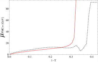
Figure 1: The LO-PMC_∞ (Solid Red) and the NLO-PMC_∞ (Dashed Black) scales for thrust.

We notice that the two PMC_∞ scale have similar behaviors in the range $(1-T)<0.33$ and the LO-PMC_∞ scale agrees with the PMC scale used in shengquan . This method totally eliminates both the ambiguity in the choice of the renormalization scale and the scheme dependence at all orders in QCD.

.6 NNLO Thrust distribution results

We use here the results of Ref. weinzierl1 ; weinzierl2 and for the running coupling $\alpha_{s}(Q)$ we use the RunDec program rundec . In order to normalize consistently the thrust distribution we expand the denominator in $\alpha_{0}\equiv\alpha_{s}(\mu_{0})$ while the numerator has the couplings renormalized at different PMC_∞-scales $\alpha_{I}\equiv\alpha_{s}(\mu_{I})$, $\alpha_{II}\equiv\alpha_{s}(\tilde{\mu}_{II})$. We point out here that the proper normalization would be given by the integration of the total cross section after renormalization with the PMC_∞ scales, nonetheless since the PMC_∞ prescription involves only absorption of higher order terms into the scales the difference would be within the accuracy of the calculations, i.e. $\sim\mathcal{O}(\alpha_{s}^{4}(\mu_{0}))$. The experimentally measured thrust distribution is normalized to the total hadronic cross section $\sigma_{tot}$ as follows:

$$\frac{1}{\sigma_{tot}}\!\frac{Od\sigma(\mu_{I},\mu_{II},\mu_{0})}{dO}=\left\{\overline{\sigma}_{I}+\overline{\sigma}_{II}+\overline{\sigma}_{III}+{\cal O}(\alpha_{s}^{4})\right\},$$ (24)

where

$$\sigma_{tot}=\sigma_{0}\left(1+\frac{\alpha_{s}(\mu_{0})}{2\pi}A_{tot}+\left(\frac{\alpha_{s}(\mu_{0})}{2\pi}\right)^{2}B_{tot}+O\left(\alpha_{s}^{3}\right)\right)$$

is the total integrated cross section and the $A_{\mathit{tot}},B_{\mathit{tot}}$ are:

$$A_{\mathit{tot}} = \frac{3}{2}C_{F};$$ (25)

$$B_{\mathit{tot}} = \frac{C_{F}}{4}N_{c}+\frac{3}{4}C_{F}\frac{\beta_{0}}{2}(11-8\zeta(3))-\frac{3}{8}C_{F}^{2}.$$ (26)

The normalized subsets in the region $(1-T)<0.33$ are then:

$$\overline{\sigma}_{I} = A_{\mathit{Conf}}\frac{\alpha_{I}}{2\pi}$$

$$\overline{\sigma}_{II} = \!\!\!\left(B_{\mathit{Conf}}+\eta A_{\mathit{tot}}A_{\mathit{Conf}}\right)\!\!\left(\frac{\alpha_{II}}{2\pi}\right)^{\!2}\!\!\!-\!\eta A_{\text{tot}}A_{\mathit{Conf}}\!\left(\frac{\alpha_{0}}{2\pi}\!\right)^{\!2}$$

$$-A_{\text{tot}}A_{\mathit{Conf}}\frac{\alpha_{0}}{2\pi}\frac{\alpha_{I}}{2\pi}$$

$$\overline{\sigma}_{III} = \!\!\left(C_{\mathit{Conf}}\!-\!A_{\text{tot}}\!B_{\mathit{Conf}}\!-\!(B_{\text{tot}}\!-\!A_{\text{tot}}^{2})A_{\mathit{Conf}}\!\right)\!\!\left(\!\frac{\alpha_{0}}{2\pi}\!\right)^{\!3}$$

Normalized subsets for the region $(1-T)>0.33$ can be achieved simply by setting $A_{\mathit{Conf}}\equiv 0$ in the Eq. LABEL:normalizedcoeff. Within the numerical precision of these calculations there is no evidence of the presence of spurious terms, such as UV-finite $N_{f}$ terms up to NNLO monni . These terms must be rather small or comparable with numerical fluctuations. Besides we notice a small rather constant difference between the iCF-predicted and the calculated coefficient for the $N_{f}^{2}$-color factor of Ref. weinzierl1 which might be addressed to a $N_{f}^{2}$ UV-finite coefficient or possibly to statistics. This small difference must be included in the conformal coefficient and it has a complete negligible impact on the total thrust distribution.

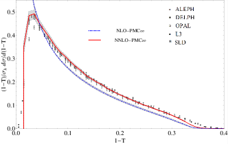
Figure 2: The thrust distribution under the PMC_∞ at NLO (DotDashed Blue) and at NNLO (Solid Red). The experimental data points are taken from the ALEPH, DELPHI,OPAL, L3, SLD experiments aleph ; delphi ; opal ; l3 ; sld . The shaded area shows theoretical errors for the PMC_∞ predictions at NLO and at NNLO.

In Fig.2 we show the thrust distribution at NLO and at NNLO with the use of the PMC_∞ method. Theoretical errors for the thrust distribution at NLO and at NNLO are also shown (the shaded area). Conformal quantities are not affected by a change of renormalization scale. Thus the errors shown give an evaluation of the level of conformality achieved up to the order of accuracy and they have been calculated using standard criteria, i.e. varying the remaining initial scale value in the range $\sqrt{s}/2\leq\mu_{0}\leq 2\sqrt{s}$. Using the same definition of the parameter $\bar{\delta}$ as in Ref. gehrmannthrust , we have in the interval $0.<(1-T)<0.33$ an average error of $\bar{\delta}\simeq 3.54\%$ and $1.77\%$ for the thrust at NLO and at NNLO respectively. A larger improvement has been calculated in the range $0.<(1-T)<0.42$ from $\bar{\delta}\simeq 7.36\%$ to $1.95\%$ from NLO to the NNLO accuracy with the PMC_∞.

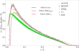
Figure 3: The thrust distribution at NNLO under the Conventional (Dashed Black), the PMC($\mu$_LO) (DotDashed Blue) and the PMC_∞ (Solid Red). The experimental data points are taken from the ALEPH, DELPHI,OPAL, L3, SLD experiments aleph ; delphi ; opal ; l3 ; sld . The shaded areas show theoretical errors predictions at NNLO and they have been calculated varying the remaining initial scale value in the range $\sqrt{s}/2\leq\mu_{0}\leq 2\sqrt{s}$.

In Fig.3 a direct comparison of the PMC_∞ with the the Conventional Scale Setting results (obtained in weinzierl1 and gehrmannthrust gehrmannshapes1 ) is shown. In addition we have shown also the results of the first PMC approach used in shengquan that we indicate as PMC($\mu$_LO) extended to the NNLO accuracy. In this approach the last unknown PMC scale $\mu$_NLO of the NLO has been set to the last known PMC scale $\mu$_LO of the LO, while the NNLO scale $\mu$_NNLO$\equiv\mu_{0}$ has been left unset and varied in the range $\sqrt{s}/2\leq\mu_{0}\leq 2\sqrt{s}$. This analysis has been performed in order to show that the procedure of setting the last unknown scale to the last known one leads to stable and precise results and is consistent with proper PMC method in a wide range of values of the $(1-T)$ variable.

$\bar{\delta}[\%]$	Conv.	PMC($\mu$LO)	PMC∞
$0.10<(1-T)<0.33$	6.03	1.41	1.31
$0.21<(1-T)<0.33$	6.97	2.19	0.98
$0.33<(1-T)<0.42$	8.46	-	2.61
$0.00<(1-T)<0.33$	5.34	1.33	1.77
$0.00<(1-T)<0.42$	6.00	-	1.95

Table 1: Average error, $\bar{\delta}$, for NNLO Thrust distribution under Conventional, PMC($\mu$_LO) and PMC_∞ scale settings calculated in different ranges of values of the $(1-T)$ variable.

Average errors calculated in different regions of the spectrum are reported in Table 1. From the comparison with the Conventional Scale Setting we notice that the PMC_∞ prescription significantly improves the theoretical predictions. Besides, results are in remarkable agreement with the experimental data in a wider range of values ( $0.015\leq 1-T\leq 0.33$) and they show an improvement of the PMC$(\mu_{LO})$ results when the two-jets and the multi-jets regions are approached, i.e. the region of the peak and the region $(1-T)>0.33$ respectively. The use of the PMC_∞ approach on perturbative thrust QCD-calculations restores the correct behavior of the thrust distribution in the region $(1-T)>0.33$ and this is a clear effect of the iCF property. Comparison with the experimental data has been improved all over the spectrum and the introduction of the $N^{3}LO$ order correction would improve this comparison especially in the multi-jet $1-T>0.33$ region. In the PMC_∞ method theoretical errors are given by the unknown intrinsic conformal scale of the last order of accuracy. We expect this scale not to be significantly different from that of the previous orders. In this particular case, as shown in Eq.LABEL:normalizedcoeff, we have also a dependence on the initial scale $\alpha_{s}(\mu_{0})$ left due to the normalization and to the regularization terms. These errors represent the 12.5% and 1.5% respectively of the whole theoretical errors in the range $0<(1-T)<0.42$ and they could be improved by means of a correct normalization.

.7 NNLO C-parameter distribution results

The same analysis applies straightforwardly to the C-parameter distribution including the regularizing $\eta$ parameter which has been set to the same value $3.51$. The same scales of Eq.16 and Eq.21 apply to the C-parameter distribution in the region $0<C<0.75$ and in the region $0.75<C<1$. In fact, due to kinematical constraints that set the $A_{\mathit{Conf}}=0$, we have the same iCF effect also for the C-parameter. Results for the C-parameter scales and distributions are shown in Fig.4 and Fig.5 respectively.

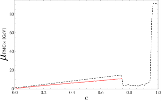
Figure 4: The LO-PMC_∞ (Solid Red) and the NLO-PMC_∞ (Dashed Black) scales for C-parameter.

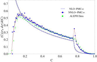
Figure 5: The C-parameter distribution under the PMC_∞ at NLO (DotDashed Blue) and at NNLO (Dashed Red). Blue points indicate the NNLO-PMC_∞ thrust distribution obtained with $\mu_{III}=\mu_{0}=M_{Z_{0}}$. The experimental data points (Green) are taken from the ALEPH experiment aleph . Dashed lines of the NNLO distribution show fits of the theoretical calculations with interpolating functions for the values of the remaining initial scale $\mu_{0}=2M_{Z_{0}}$ and $M_{Z_{0}}/2$. The shaded area shows theoretical errors for the PMC_∞ predictions at NLO and at NNLO calculated varying the remaining initial scale value in the range $\sqrt{s}/2\leq\mu_{0}\leq 2\sqrt{s}$.

Theoretical errors have been calculated, as in the previous case, using standard criteria and results indicate an average error over the whole spectrum $0<(C)<1$ of the C-parameter distribution at NLO and at NNLO of $\bar{\delta}\simeq 7.26\%$ and $2.43\%$ respectively.

$\bar{\delta}$[%]	Conv.	PMC($\mu$LO)	PMC∞
$0.00<(C)<0.75$	4.77	0.85	2.43
$0.75<(C)<1.00$	11.51	3.68	2.42
$0.00<(C)<1.00$	6.47	1.55	2.43

Table 2: Average error ,$\bar{\delta}$, for NNLO C-parameter distribution under Conventional, PMC($\mu$_LO) and PMC_∞ scale settings calculated in different ranges of values of the $(C)$ variable.

A comparison of average errors according to the different methods is shown in Table2. Results show that the PMC_∞ improves the NNLO QCD predictions for the C-parameter distribution all over the spectrum.

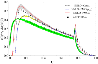
Figure 6: The NNLO C-parameter distribution under the Conventional Scale Setting (Dashed Black), the PMC($\mu$_LO) (DotDashed Blue ) and the PMC_∞ (Solid Red). The experimental data points (Black) are taken from the ALEPH experiment aleph . The shaded area shows theoretical errors predictions at NNLO calculated varying the remaining initial scale value in the range $\sqrt{s}/2\leq\mu_{0}\leq 2\sqrt{s}$.

Comparison of the distributions calculated with the Conventional Scale Setting, the PMC($\mu$_LO) and the PMC_∞ is shown in Fig.6. Results for the PMC_∞ show a remarkable agreement with the experimental data away from the regions $C<0.05$ and $C\simeq 0.75$. The errors due to the normalization and to the regularization terms (Eq.LABEL:normalizedcoeff) are respectively the $8.8\%$ and $0.7\%$ of the whole theoretical errors. The perturbative calculations could be further improved using a correct normalization and also by introducing the large logarithms resummation technique in order to extend the perturbative regime.

.8 Comment on the last PMC_∞ scale

We have shown in this article a property of the perturbative QCD corrections which is consistent with the MC results of single variable distributions for $e^{+}e^{-}\rightarrow 3jets$. This property leads to the PMC_∞ : an infinite-order scale setting based on the Principle of Maximum Conformality method. The PMC_∞ method preserves the iCF form and is void of ambiguities. The absence of ambiguities in PMC_∞ is clearly shown hereby simply noticing that the new scale at a each order is fixed by considering the $\beta_{0}$- i.e. $N_{f}$-term and no other term is needed in agreement with the iCF parametrization. Thus PMC_∞ scale fixing procedure is constrained by the iCF form and the choice of the scales is totally free of any ambiguity. The only unknown scale which remains unfixed apparently, is the one given by the last order of accuracy. In this article this scale has been fixed to the $\mu_{III}=\mu_{0}=M_{Z_{0}}$ for sake of a consistent comparison with the Conventional method. We remark that the last ”unknown” PMC scale can be fixed to the last known one. In fact, as we have also shown in this article, in general the differences between two consecutive scales are not only rather small, but the use of the method PMC($\mu$_LO) leads to precise and consistent results in a wide range of the perturbative region as reported in Table 1 and 2 of the previous sections. In the case of the thrust and C-parameter distributions calculated at NNLO with the PMC_∞, the differences between the $\mu_{III}=M_{Z_{0}}$ or $\mu_{III}=\tilde{\mu}_{II}$ are also negligible and these differences are totally confined within the errors shown for the distributions in the perturbative region. Given the Conformal Limit of the Eq. LABEL:nlimit, the last term in the iCF determines the level of conformality reached by the expansion and the whole scale dependence is confined in the coupling. As previously shown, this term is the main source of the uncertainties (as also reported in the Ref.Chawdhry:2019uuv ) and a further investigation regarding the regularization method applied here would be necessary in order to extend the procedure to all orders.

I Conclusions

We have introduced here the iCF Intrinsic Conformality, a parametrization which preserves exactly the scale invariance of an observable. We have shown a new method to solve the conventional renormalization scale ambiguity in QCD named PMC_∞ which preserves the iCF and leads to conformal renormalization scales. This method agrees with the PMC at LO and and it applies to abservables especially in cases of a clearly manifested iCF, as for example in the case of the event shape variables. We have presented a new procedure to identify the iCF/PMC_∞-coefficients at all orders which can be applied to either numerical or analytical calculations. The PMC_∞ has been applied to the NNLO thrust and C-parameter distributions and the results show perfect agreement with the experimental data. The evaluation of theoretical errors using standard criteria show that the PMC_∞ significantly improves the theoretical predictions all over the spectra of the shape variables. The PMC_∞ method eliminates the renormalon growth $\alpha_{s}^{n}\beta_{0}^{n}n!$, the scheme dependence and all the uncertainties related to the scale ambiguity up to the order of accuracy. The iCF/PMC_∞ scales are identified by the lowest order logarithm related to the $\beta_{0}$-term at each order and all the physics of the process is contained in the conformal coefficients. This is in complete agreement with QED and with the Gell-Mann and Low scheme qed ; huet . We have discussed why iCF should be considered a strict requirement for a theory in order to preserve the scale invariance of the observables and we have shown that iCF is consistent with the single variable thrust and C-parameter distributions. We point out that other conformal aspects of QCD resulting from different sectors such as Commensurate Scale Relations-CSR csr or dual theories as AdS/CFT ads1 might also be related to the Intrinsic Conformality. We underline that the iCF property in a theory would have two main remarkable consequences: first, it shows what is the correct coupling constant at each order as a function of the conformal intrinsic scale $\mu_{N}$, and second, since only the conformal and the $\beta_{0}$ coefficients need to be identified in the observables at each order, by means of the PMC_∞ method the iCF would reveal its predictive feature for the coefficients of the higher order color factors. We point out that in many cases the implementation of the iCF in a multi-loop calculations procedure would lead to a significant reduction of the color factors coefficients and it would speed up the calculations for higher order corrections.

Acknowledgements: We thank Francesco Sannino for useful discussions. L.D.G. wants to thank the SLAC theory group for its kind hospitality and support. This work was also supported by the Department of Energy Contract No. DE-AC02-76SF00515.
SLAC-PUB-17511.

References

- (1) D. Maitre et al., PoS E PS-HEP2009, 367 (2009) [arXiv:0909.4949 [hep-ph]].
- (2) P. M. Stevenson, Phys. Rev. D 23, 2916 (1981).
- (3) G. Grunberg, Phys. Lett. B 95, 70 (1980).
- (4) G. Kramer and B. Lampe, Z. Phys. A 339, 189-193 (1991).
- (5) S. J. Brodsky and L. Di Giustino, Phys. Rev. D 86, 085026 (2012).
- (6) S. J. Brodsky and X. G. Wu, Phys. Rev. D 85, 034038 (2012).
- (7) S. J. Brodsky and X. G. Wu, Phys. Rev. Lett. 109, 042002 (2012).
- (8) M. Mojaza, S. J. Brodsky and X. G. Wu, Phys. Rev. Lett. 110, 192001 (2013).
- (9) S. J. Brodsky, M. Mojaza and X. G. Wu, Phys. Rev. D 89, 014027 (2014).
- (10) X. G. Wu, J. M. Shen, B. L. Du, X. D. Huang, S. Q. Wang and S. J. Brodsky, Prog. Part. Nucl. Phys. 108, 103706 (2019)
- (11) X. G. Wu, Y. Ma, S. Q. Wang, H. B. Fu, H. H. Ma, S. J. Brodsky and M. Mojaza, Rept. Prog. Phys. 78, 126201 (2015)
- (12) X. G. Wu, S. J. Brodsky and M. Mojaza, Prog. Part. Nucl. Phys. 72, 44 (2013)
- (13) M. Gell-Mann and F. E. Low, Phys. Rev. 95, 1300 (1954).
- (14) S. J. Brodsky and P. Huet, Phys. Lett. B 417, 145 (1998).
- (15) S. J. Brodsky, J. R. Ellis, E. Gardi, M. Karliner and M. A. Samuel, Phys.Rev. D56, 6980-6992 (1997).
- (16) V. Del Duca, C. Duhr, A. Kardos, G. Somogyi, Z. Ször, Z. Tröcsanyi and Z. Tulipánt, Phys. Rev. D 94, 074019 (2016).
- (17) V. Del Duca, C. Duhr, A. Kardos, G. Somogyi and Z. Tröcsanyi, Phys. Rev. Lett. 117, 152004 (2016).
- (18) S. J. Brodsky, G. P. Lepage and P. B. Mackenzie, Phys.Rev. D 28, 228(1983).
- (19) M. Beneke, Phys. Rept. 317, 1 (1999).
- (20) S. Weinzierl, JHEP 0906, 041 (2009).
- (21) S. Weinzierl, Phys. Rev. Lett. 101, 162001 (2008).
- (22) M. Binger, S. J. Brodsky, Phys.Rev. D 74, 054016 (2006)
- (23) S. Catani, G. Turnock, B.R. Webber and L. Trentadue, Phys. Lett. B 263, 491 (1991).
- (24) S. Catani, L. Trentadue, G. Turnock and B.R. Webber, Nucl. Phys. B 407, 3 (1993).
- (25) S. Catani, M. L. Mangano, P. Nason, L. Trentadue, Nucl.Phys. B478, 273-310 (1996).
- (26) U. Aglietti, L. Di Giustino, G. Ferrera, L. Trentadue, Phys.Lett. B651 275-292 (2007).
- (27) A. Banfi, H. McAslan, P. F. Monni and G. Zanderighi, JHEP 1505, 102 (2015).
- (28) R. Abbate, M. Fickinger, A. H. Hoang, V. Mateu and I. W. Stewart, Phys. Rev. D 83, 074021 (2011).
- (29) S. Q. Wang, S. J. Brodsky, X. G. Wu, L. Di Giustino, Phys.Rev. D 99, 114020 (2019).
- (30) K. G. Chetyrkin, J. H. Kuhn and M. Steinhauser, Comput. Phys. Commun. 133, 43 (2000).
- (31) T. Gehrmann, N. H fliger and P. F. Monni, Eur.Phys.J. C 74, n.6 2896 (2014)
- (32) A. Gehrmann-De Ridder, T. Gehrmann, E. W. N. Glover and G. Heinrich, Phys. Rev. Lett. 99, 132002 (2007).
- (33) A. Gehrmann-De Ridder, T. Gehrmann, E. W. N. Glover and G. Heinrich, JHEP 0712, 094 (2007).
- (34) H. A. Chawdhry and A. Mitov, Phys. Rev. D 100, no. 7, 074013 (2019).
- (35) H. J. Lu and S. J. Brodsky, Nucl.Phys.Proc.Suppl. 39BC , 309-311 (1995).
- (36) A. Heister et al. [ALEPH Collaboration], Eur. Phys. J. C 35, 457 (2004).
- (37) J. Abdallah et al. [DELPHI Collaboration], Eur. Phys. J. C 29, 285 (2003).
- (38) G. Abbiendi et al. [OPAL Collaboration], Eur. Phys. J. C 40, 287 (2005).
- (39) P. Achard et al. [L3 Collaboration], Phys. Rept. 399, 71 (2004).
- (40) K. Abe et al. [SLD Collaboration], Phys. Rev. D 51, 962 (1995).
- (41) S. Q. Wang, S. J. Brodsky, X. G. Wu, J. M. Shen, L. Di Giustino, Phys. Rev. D 100, 094010 (2019).
- (42) S. J. Brodsky and G. F. de T ramond, Phys. Lett. B582 , 211-221 (2004).