Plasmoid formation in global GRMHD simulations and AGN flares
Abstract
One of the main dissipation processes acting on all scales in relativistic jets is thought to be governed by magnetic reconnection. Such dissipation processes have been studied in idealized environments, such as reconnection layers, which evolve in merging islands and lead to the production of “plasmoids”, ultimately resulting in efficient particle acceleration. In accretion flows onto black holes, reconnection layers can be developed and destroyed rapidly during the turbulent evolution of the flow. We present a series of two-dimensional general-relativistic magnetohydrodynamic simulations of tori accreting onto rotating black holes focusing our attention on the formation and evolution of current sheets. Initially, the tori are endowed with a poloidal magnetic field having a multi-loop structure along the radial direction and with an alternating polarity. During reconnection processes, plasmoids and plasmoid chains are developed leading to a flaring activity and hence to a variable electromagnetic luminosity. We describe the methods developed to track automatically the plasmoids that are generated and ejected during the simulation, contrasting the behaviour of multi-loop initial data with that encountered in typical simulations of accreting black holes having initial dipolar field composed of one loop only. Finally, we discuss the implications that our results have on the variability to be expected in accreting supermassive black holes.
keywords:
black hole physics, accretion, accretion discs, magnetic reconnection1 Introduction
Relativistic jets are observed in high-energy sources, from gamma-ray bursts (GRB) to active galactic nuclei (AGNs). They can be launched from magnetic processes around black holes (Blandford & Znajek, 1977; Blandford & Payne, 1982) and the numerical simulation of these processes has now reached significant maturity (see, e.g., Rezzolla et al. 2011; Event Horizon Telescope Collaboration et al. 2019). The magnetic-field topology plays a central role in determining the structure of the outflows from these systems and is fundamental for energy dissipation through various magnetohydrodynamic (MHD) instabilities and magnetic reconnection.
Accretion in magnetized disks is believed to be driven by the magneto-rotational instability (MRI) (Balbus & Hawley, 1991), where the advection of plasma and magnetic fields provides the main ingredients to launch magnetized winds and jets. Magnetically dominated jets accelerate efficiently the bulk of the plasma while keeping much of the energy stored into the field itself (Komissarov et al., 2009; Lyubarsky, 2009; Tchekhovskoy et al., 2009). Under these conditions, magnetic reconnection represents an efficient way to dissipate some of this magnetic energy and it has been proposed to explain GRB and AGN emission (di Matteo, 1998; Zhang & Shu, 2011; Giannios & Sironi, 2013; Dionysopoulou et al., 2015)
Large-scale magnetized jets that are produced from accretion flows around black holes tend to have a variable electromagnetic power. This is due to the intrinsically turbulent nature of the accretion process that, in turn, produces and advects onto the black hole magnetic-field loops of different polarity, whose interaction provides the sites for formation of current sheets. These magnetic loops can emerge in the surface of the disk due to buoyancy like the Rayleigh-Taylor instability (Parker, 1966), and can change the topology of the magnetic field throughout the jet. Furthermore, because of their turbulent genesis, these will not respect any symmetry across the equatorial plane and may therefore lead to differences in the wind properties above and below the equatorial plane (Kadowaki et al., 2018).
Previous studies have established the importance of the magnetic-field configuration for the production of a steady outflow and more specifically its power. The nested-loop poloidal magnetic-field structure, which is the one normally adopted as initial data to model magnetized accretion onto black holes (Gammie et al., 2004; De Villiers et al., 2005; McKinney, 2006), has been shown to produce relativistic jets. Depending on the initial strength of the magnetic field, the efficiency of the energy extraction from the black hole can go beyond efficiency, thus producing very powerful outflows in the case of magnetically arrested disks (MAD, Igumenshchev et al. 2003; Narayan et al. 2003; Tchekhovskoy et al. 2011).
In addition to the nested-loops, different magnetic-field configurations have also been studied, leading to a picture in which jet launching is especially sensitive to the initial magnetic-field geometry (Beckwith et al., 2008, 2009). More specifically, the outflows resulting from the accretion can vary depending on the the initial magnetic-field configuration, going from jets that are weak and mostly turbulent, to powerful and collimated ones (Beckwith et al., 2008; McKinney & Blandford, 2009; McKinney et al., 2012; Narayan et al., 2012; Liska et al., 2018; Event Horizon Telescope Collaboration et al., 2019). A particularly interesting configuration that has been studied recently is one in which loops of alternating polarity are periodically advected to the black hole (Parfrey et al., 2015). Such configurations with a region of alternating polarity can be also produced naturally in accretion flows around black holes (Contopoulos & Kazanas, 1998; Contopoulos et al., 2015, 2018), and lead rather naturally to the development of regions of alternating magnetic-field polarity.
Recent observations of rapid variability of X-ray/gamma-ray flares in blazars with timescales from several minutes to a few hours pose severe constraints on the particle acceleration timescale and the size of the emission region (e.g., Aharonian et al. 2007; Albert et al. 2007). From observations, fast variable flares may come from a small region with a size of the order of a few Schwarzschild radii, launching fast moving “needles” within a slower jet or from jet within a jet (Levinson, 2007; Begelman et al., 2008; Ghisellini & Tavecchio, 2008; Giannios et al., 2009). Flares also require very rapid particle acceleration.
Throughout the jet, instabilities – and the associated turbulence – can can provide rather naturally the sites for the generation of current sheets and hence for the occurrence of magnetic reconnection. These configurations of current sheets structured by large sheets of alternating magnetic-field polarity have been studied and found to be very efficient in particle acceleration (see, e.g., Kagan et al. 2015 for a review). Quite generically the initial configuration fragments at the current sheet layer and produces chains of magnetic “plasmoids” (or “magnetic islands”) (Loureiro et al., 2007; Uzdensky et al., 2010; Fermo et al., 2010; Huang & Bhattacharjee, 2012; Loureiro et al., 2012; Takamoto, 2013). We recall that plasmoids are quasi-spherical regions that contain relativistic particles and have a large magnetization, that is a large ratio between the magnetic and rest-mass energies. Magnetic reconnection and plasmoid formation has been extensively studied in Particle-in-Cell (PIC) simulations, which have confirmed that magnetic reconnection in relativistic regimes to be very efficient in accelerating charged particles (Sironi & Spitkovsky, 2014; Guo et al., 2014, 2015; Werner et al., 2016; Sironi et al., 2016; Li et al., 2017b; Kagan et al., 2018; Petropoulou et al., 2019). Plasmoids produced from magnetic reconnection events can be studied systematically in a statistical manner (Petropoulou et al., 2018) and have been introduced to explain flaring activity and AGN emission (Petropoulou et al., 2016; Zhang et al., 2018; Christie et al., 2019).
In view of the potential importance of plasmoid formation and evolution in the dynamics and energetics of relativistic jets, we have here carried out the first steps to asses and measure such properties in rather realistic general-relativistic conditions of accretion flows around black hole. The main goal of this work is, therefore, is to build and explore those magnetic-field geometries that are more likely to lead to the formation of current sheets and therefore to magnetic reconnection.
To this scope, we have performed a series of two-dimensional general-relativistic ideal-MHD simulations exploring initial magnetic fields having different coherence length and topology, and assessing the impact that these initial conditions have on the production rate of plasmoids in each case. More specifically, we initialize the accretion torus with a varying number of poloidal magnetic loops of alternating polarity and contrast the results of the corresponding simulations with those obtained with the nested-loop setup typically used in the literature. Special attention is paid to the formation of current sheets, to the occurrence of magnetic reconnection, and to the consequent production of plasmoids and plasmoid chains. Overall, we find that reconnection layers are rapidly developed and destroyed in the vicinity of the black hole. In such reconnection layers, plasmoids are generated and, in some cases, accelerated to large energies, thus becoming candidates to explain the flaring activity in AGNs.
This paper is organized as follows: in Section 2 we present the overview of the simulations, the numerical setup 2.1, a brief comparison of the initial models 2.2 and the specifics of the models where reconnection occurs 2.3. Section 3 discussed in more detail the production of plasmoids through the reconnection layers and their evolution. Finally, we summarize and present a discussion about the results in Section 4.
2 Numerical details and model comparison
2.1 Numerical setup
For our simulations, we employ BHAC (Porth et al., 2017), which solves the equations of general-relativistic ideal MHD using second-order high-resolution shock-capturing finite-volume methods. The code has been employed in a number of investigations, e.g., (Mizuno et al., 2018; Nathanail et al., 2019), and has been carefully tested and compared with codes with similar capabilities Porth et al. (2019). BHAC solves the general-relativistic MHD equations
| (1) | ||||
| (2) | ||||
| (3) |
where is the rest-mass density, the fluid -velocity, the energy momentum tensor and is the dual of the Faraday tensor. Our simulations are performed in two spatial dimensions. The code makes uses of fully adaptive mesh-refinement (AMR) techniques and of the constrained-transport method (Del Zanna et al., 2007) to preserve a divergence-free magnetic field (Olivares et al., 2019).
As initial data we consider an axisymmetric equilibrium torus with constant specific angular momentum (Fishbone & Moncrief, 1976) around a Kerr black hole with a dimensionless spin of , where and are the angular momentum and mass, respectively. The inner radius of the torus is set to be and the outer radius , where is the gravitational radius (we use units in which ).
As mentioned above, the initial magnetic field is buried in the torus and purely poloidal, but chosen so as to have four different topologies consisting of a series of nested loops with varying polarity along the radial direction. This is achieved by making use of a vector potential with the form
| (4) | |||
where is the maximum rest-mass density in the torus and the parameters and set the number and the characteristic lengthscale (and hence the polarity) of the poloidal loops inside the torus respectively and thus are varied to produce the desirable initial magnetic-field topologies.
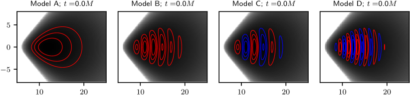
Overall, we have considered four different models whose initial magnetic-field structure is reported in Fig. 1. In most of the runs we use a logarithmic grid in the radial direction so that the domain extends to . The various parameters used are summarized in Table 1, where the last three columns refer to the resolution of the simulations, which is different for the various setups because of the varying characteristic lengthscales in the. Most of the figures discussed hereafter will refer to simulations performed with the highest resolution: i.e., at the base resolution for B, at the base resolution for Models A, C and D.
| model | |||||||
|---|---|---|---|---|---|---|---|
| (base res.) | (2 base res.) | (4 base res.) | (6 base res.) | ||||
| Model A | |||||||
| Model B | |||||||
| Model C | |||||||
| Model D |
The first model, Model A, includes the typical nested loop magnetic-field topology. Model B consists of a multi-loop structure where all loops have the same polarity. The last two models have a multi-loop structure where each loop has an alternate polarity. The loops of Model B and Model C have a similar width, whereas in Model D the loops have a smaller size. For the last two models, several resolutions where used to check the impact on the activation and saturation of the MRI, these are discussed in the Appendix B. Furthermore, for the two models with alternate polarity loops, Model C and Model D, we run a set of simulations. The simulation runs are evolved up to . Such a timescale is sufficiently long to capture all the important and distinctive features of each simulation and is sufficiently short that the we need not to be concerned about the decaying poloidal magnetic field, which takes place in axisymmetry as a consequence of the decay of turbulence (Cowling, 1933; Sa̧dowski et al., 2015).
2.2 Model comparison
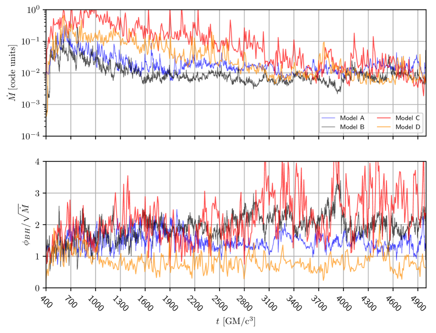
Since our focus here is to determine and highlight those features in the plasma dynamics that emerge when considering different initial magnetic-field topologies, we first discuss the main differences among the four models. A particularly useful quantity in this respect are the amount of rest-mass and magnetic field accreted onto the black hole, namely, the mass-accretion rate and the accreted magnetic flux. The former is measured as
| (5) |
and is shown for all models in the upper panel of Fig. 2. Note that after a time of , the accretion rate in all models relaxes to a roughly constant value. In Model C and D the mass-accretion rate remains roughly constant till , in the high-resolution runs, thus reflecting an essentially stationary turbulent state in the torus.
Similarly, we define magnetic flux accreted across the event horizon as
| (6) |
and show its normalized value in the lower panel of Fig. 2 for all of the models considered. Note that for Model A the normalized magnetic flux is roughly constant in time and it is far below the saturation limit that is normally taken for a MAD configuration (within the units adopted here Tchekhovskoy et al. (2011)). This net magnetic flux is a prerequisite for energy extraction from the black hole (Blandford & Znajek, 1977). What the simulations reveal is that magnetic flux of one polarity is brought towards the horizon of the black hole but also that magnetic flux of the opposite polarity reaches the vicinity of the horizon, thus annihilating the previous one and reducing the overall flux across the horizon. Fluctuations in this overall behaviour are stronger in the two cases where the initial loops have larger width, i.e., Models B and C. In these cases, the evolution of the magnetic flux shows both a short dynamical timescale – as magnetic flux is brought to the horizon – but also a longer timescale reflecting the amount of time needed for the whole loop to be partly annihilated and as a result reduce the magnetic flux on the horizon. Overall, the magnetic flux in Models B and C is at all times higher than in the other two cases. It is important to note here that even if the magnetic flux in Model C is three or four times larger than Model A, a magnetic funnel is never produced due to the continuous magnetic flux annihilation.
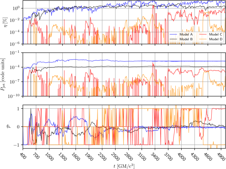
All models considered produce outflows that give off energy at infinity. This can be measured through the energy flux that passes through a 2-sphere placed at
| (7) |
where the integrand in (7) is set to zero if everywhere on the integrating surface . The efficiency of the jet is then defined as
| (8) |
and can become larger than unity. Lastly, in order to measure the contribution, and difference in the power from the upper and the lower jet we introduce the jet asymmetry
| (9) |
where and are the powers of the upper and lower jets, respectively. Clearly, when the upper jet dominates, for power releases dominated by the lower jet, while refers to a symmetric jet emission. Note that we set when the power of both the upper and the lower jets are zero because nowhere on the integrating surface is the condition satisfied.
All of these quantities are shown in the three panels of Fig. 3 for the various models considered. In particular, it is possible to note that Models A and B produce steady jet structures where the efficiency of the jet and the power of the jet are roughly constant in time (see upper and middle panels of Fig. 3). Furthermore, the difference of the upper and lower jet is at all times close to zero (lower panel of Fig. 3), which means that both jets contribute equally to the overall power. Models A and B are quite similar in jet power and efficiency. This is because the small-scale field between the loops of Model B reconnect and yield a topology similar to Model A. The magnetic field in Models C and D, on the other hand, do not reconnect so efficiently and the long-term dynamics is governed by the small-scale seed fields. Furthermore, for Models C and D there is a strong variability in the power of the outflows and as we will see below they do not even form steady structures. It is important to note that even if they do not produce jets, in the usual form, they exhibit an intense flaring activity. It is tempting to relate the timescale of the flaring activity in Models C and D with the characteristic lengthscale of the initial magnetic loops. In the case of Model C, the loops have a larger coherence lengthscale which is then imprinted on the subsequent turbulent flow and leads to typical times between flares to be longer (Fig. 3). Similarly, for Model D, where the loops are smaller the power is highly variable and changes in a smaller timescale.
Using the mass estimate for Sgr A∗ coming from Boehle et al. (2016), this flaring activity has a time span from minutes to tens of minutes, and could therefore be correlate with the recent observations of the X-ray activity of Sgr A∗ (Haggard et al., 2019). Some variability is seen in well structured jets, however in the case of Models C and D variability is very intense and the power during the flare can vary up to two orders of magnitude in a time span of tens of minutes for Sgr A∗ (Do et al., 2019).
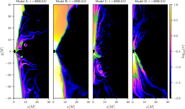
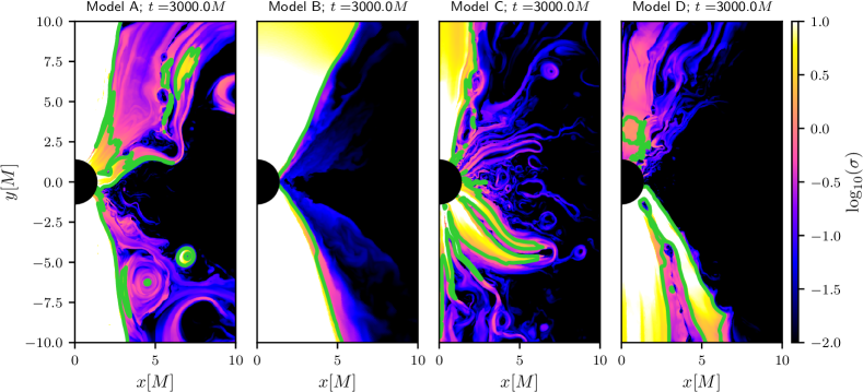
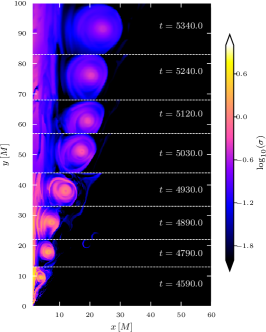
In order to delimit and visualize the region representing the jet, we use the magnetization parameter, , and define as jet the low-density, strong magnetic-field region with . In Fig. 4 we plot for all models in a logarithmic colorcode and at time . Note that the jet is well structured in Model A and that this structure is stationary throughout the simulation. This is not particularly surprising and has been shown to occur in numerous simulations over the last decade, (see, e.g., De Villiers et al., 2003; McKinney & Gammie, 2004; Porth et al., 2019).
Similarly, in the case of Model B, where the initial magnetic loops are of the same polarity, a similar magnetized region is observed, which however has a reduced magnetization and a slightly different shape. The magnetization is less than the previous model, with , but clearly forms a jet structure. On the other hand, in the other two case for Models C and D, no stationary magnetized structure is produced during the timescale of the simulations. At all times, in fact, the funnel structure varies due as reflected by the variability in the magnetic flux on the black-hole horizon. Furthermore, the advection of magnetic loops of varying polarity from the turbulent disc does no longer show a symmetry across the equatorial plane. As a consequence, at some times a magnetized region can be seen in the upper hemisphere, whereas at other times in the lower hemisphere. Another important feature that can be identified in these plots, is the formation of “plasmoids”, whose properties we will discuss in more detail below. magnetization.
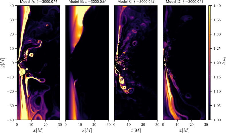
Because of the very large magnetization reached in models Model A and B the fluid in these funnel regions is expected to be accelerated and to become gravitationally unbound. In order to ascertain whether this is the case, we employ the Bernoulli criterion, according to which a fluid element is defined to be unbound if it has , where is the specific enthalpy of the fluid (Rezzolla & Zanotti, 2013)111A discussion between different definitions for the unbound criterion and their comparison has been discussed by Bovard et al. (2017). Other contributions can be added to this criterion e.g., magnetic and radiative (Narayan et al., 2012; Chael et al., 2018). The hydrodynamic prescription that we use effectively underestimates the amount of unbound/outgoing material, so that the material that we identify as unbound is actually going to reach a distant observer..
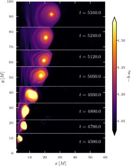
Figure 5 reports the value of the quantity for the four models considered and clearly highlights that for Models A and B, a large portion of the material in the funnel is unbound and especially the one in the jet sheath. On the other hand, when considering Models C and D, it is clear that the unbound material is not uniformly distributed, but appears in chains of plasmoids that move outwards. In particular, while Model C exhibits a larger number of out-going unbound plasmoids, which could be responsible of a subsequent flaring activity, Model D shows fewer plasmoids which are also accompanied by a uniform ejection of matter. These distinct features will be further explored in the coming sections.
2.3 Magnetized regions of alternating polarity
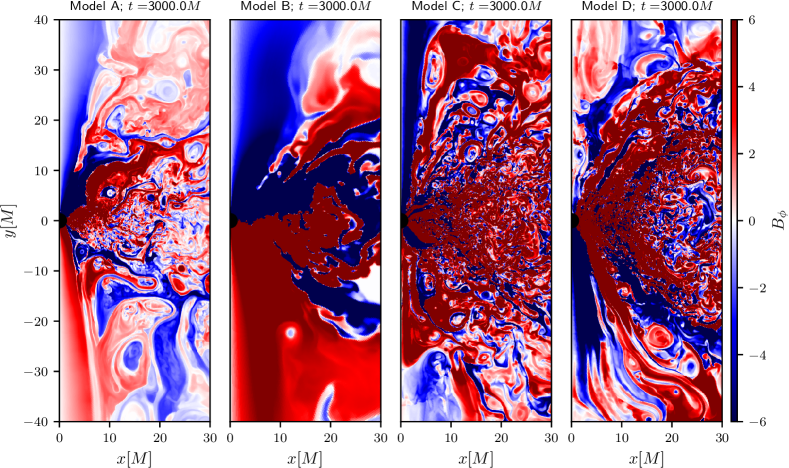
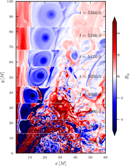
One of the most useful quantities to monitor here is the toroidal component of the magnetic field, which is initially zero but amplified exponentially by the development of the MRI. In particular, and as we will comment later on, the changes in polarity that the toroidal field experience in regions of low rest-mass density – or, equivalently, in regions of high magnetization – are closely connected to reconnection and hence to the generation of plasmoids.
To highlight the role played by the toroidal magnetic field, we show In Fig. 6 the toroidal component of the magnetic field, . The rapid change of polarity, which is highlighted in the figure by adjacent regions in blue/red, will lead to the formation of current sheets. Figure 6 shows quite remarkably how Model A and Model B differ considerably from Model C and Model D. The first two, in fact, have large regions in the torus where the toroidal magnetic field has the same polarity, while clear change of polarity lies at the limit of the torus (this is similar to the current sheet discussed and shown by Ball et al. 2018a). This phenomenology is very different from the one shown in the latter two models, where the toroidal magnetic field inside the torus has a typical coherence lengthscale of a few only. More importantly, Models C and D show that current sheets form also on the outer edges of the torus and hence close to the jet sheath. This phenomenology is absent in models A and B, and is responsible for the generation and launching of the plasmoids222Also the interior of the torus is highly turbulent region with changes of polarities that have even smaller lengthscales. However, because of the high density in the torus and and the very low magnetization, the acceleration of plasmoids via reconnection is expected to be suppressed in these regions (Li et al., 2017b).
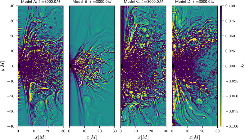
The presence of current sheets in the toroidal direction can also be appreciated through the distribution of the toroidal current , which we report in Fig. 7 for the four models and at a representative time. Note that for Model A and B, the funnel regions are essentially devoid of current sheets and exhibit almost constant and essentially zero toroidal currents. This is in contrast to what happens for Model C and D, whose funnel regions show highly variable regions of toroidal currents with changing polarities.
Combining the information from Figs. 6 and 7 with that on the unbound material in Fig. 5), it appears clear that as consecutive loops of alternating polarity are advected from the torus near the black hole, current sheets are constantly generated above and below the black hole. The conversion of magnetic energy into internal energy result from the reconnection, accelerates this material up to energies that make it become unbound.
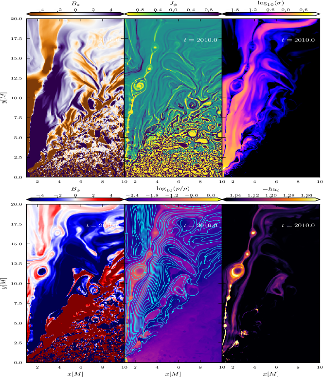
In order to have a closer look on such a region, we focus in Fig. 8 on Model D at time , where current sheets are clearly visible and easily identified. More specifically, the six panels of the figure report from left to right: , , , , , and . Poloidal magnetic-field lines in the middle panel of the second row panels, although such lines are not shown in the dense torus region for clarity. Overall, the various panels show that when going from the equatorial plane towards the polar axis, regions of different polarity appear both in the poloidal and in the toroidal magnetic field. Due to the accretion process, these regions are progressively pushed together and forced to reconnect in different sites. The reconnection layers that lie inside the torus can contribute to electron heating, but because the magnetization in such regions is very low, this material is not expected to contribute to any flaring activity. On the other hand, the reconnection layers in the polar (funnel) region, where the density is low and the magnetization is high, can be expected to be accelerate and unbind matter more efficiently (see last panel of the second row in Fig. 8) and hence represent the optimal sites to produce a flaring activity.
In the central panel of the bottom row, we report the ratio , as a guide to distinguish regions of different temperature and over-plotted in cyan, are the poloidal magnetic-field lines. Combining information from the poloidal and toroidal magnetic-field strengths it is possible to reconstruct the various regions where magnetic-field lines change polarity, thus indicating the presence of a reconnection layer. These layers can also be tracked through the azimuthal current (central panel of the upper row in Fig. 8). Plasmoids are generically formed in these reconnection layers, but a clear distinction should be made between those that eventually become unbound and the ones that do not leave the black-hole–torus system. In particular, in regions with high magnetization and high Alfvèn speed (right panel in the upper row of Fig. 8), the process of acceleration is more efficient and plasmoids generated in such regions are energized becoming unbound (right panel in the lower row of Fig. 8). On the other hand, if the magnetization is not sufficiently high, the plasmoid produced fail to be launched, as shown in the in the upper-left corners of the various panels in Fig. 8, where a reconnection layer can be clearly seen in the panels for and , but not in the panel for the Bernoulli constant . Since the magnetization in this region is almost two orders of magnitude smaller, the efficiency of the conversion of magnetic energy to internal energy is much smaller and hence does not lead to a plasmoid launching. This is also reflected by the absence in this region of an extra heating and can be clearly appreciated from the central panel in the lower row of Fig. 8, whose upper-left corner is about one order of magnitude colder.
Figure 8 shows that there are several plasmoids of various sizes that can be clearly found across the six panels. However, the large magnetic field in the main reconnection layer in the central region of Fig. 8 (i.e., at , ), one able to produce and energize a whole series of plasmoids along the current sheet, i.e., a “plasmoid chain”. By looking at the magnetization parameter (top right panel) we see that main reconnection layer responsible for the plasmoid chain lies in a region with high magnetization where and is never smaller than . This is in agreement with the results of Li et al. 2017b; Ball et al. 2018b, and highlights that reconnection layers with low magnetization, i.e., , are not efficient in producing highly energized pockets of plasma.
It is also worth remarking about the reconnection layers that are developed in Model A between the torus and the low-density regions above and below the torus. These are clearly visible in Fig. 6 and 7 (leftmost panels), where reconnection layers of alternating polarity develop further out from the funnel-jet region. The reconnection processes taking place in these regions could contribute to the heating of the local material. Also in this case, however, we do not expect these plasmoids to contribute to any flaring activity because of the low magnetization in these regions, which is .
Before closing this section, we briefly discuss the conditions for the activation of the Blandford & Znajek (1977) (BZ) mechanism to power the jet and extract energy from the rotating black hole. Following Komissarov & Barkov (2009), the critical condition for the activation of the BZ mechanism is for the Alfvèn velocity to exceed the free-fall velocity at the ergosphere. This condition, which is not straightforward to validate, effectively translates into requiring that the magnetization is at the ergosphere. Furthermore, this condition is clearly always fullfilled for Models A and B, for which the magnetization in the jet is always very high, but this is less clear for Models C and D, for which , close to the black hole, thus implying that the BZ mechanism could be quenched at times. Conversely, there are times in the dynamics of models Models C and D when the funnel region accumulates enough magnetic flux of a single polarity to exceed . This is shown, for example, in Fig. 4, which shows that the upper funnel of Model C and the lower funnel of Model D are both highly magnetized, thus with a potentially active BZ mechanism. However, because the accumulated magnetic flux varies continuously and magnetic field with opposite polarities is regularly accreted, it is difficult to build a steady jet and hence generate the physical conditions necessary for the development of a stationary BZ mechanism. This behaviour is also reflected in Fig. 2 and in particular in the upper panel, which clearly shows how the jet efficiency if always less than unity in Models C and D.
3 Dynamics of the plasmoids
Thus far we have described models where reconnection layers naturally develop as a result of the initial magnetic-field configuration embedded in the torus. These reconnection layers result in the formation of plasmoids and plasmoid chains. These quasi-spherical blobs are sometimes energized and eventually outgoing. However, this is not always the case. Other times some of these blobs are either advected and accreted by the black hole or are bound to the torus. Since unbound plasmoids are conjectured to be filled with high-energy particles and may be at the origin of flares in AGNs (Yuan et al., 2009; Giannios, 2013; Younsi & Wu, 2015; Li et al., 2017a), it is interesting to track their evolution both in terms of kinematics, (via spacetime diagrams) but also in terms of their of their thermodynamics (via the evolution of the magnetization and temperature). Note that this interest goes beyond a mere question of plasma dynamics, since, as discussed by Younsi & Wu (2015), the evolution of the physical properties of a plasmoid is essential to assess its role and contribution to a flare. For compactness, we postpone a more detailed discussion of this point to a forthcoming future study.
Finding and tracking plasmoids is however far from trivial, especially if one wants to rely on a fully automated identification and classification pipeline. To this scope, we next describe two different ways to identify individual plasmoids and track them during their evolution. A more detailed discussion on the tracking procedure can be found in the Appendix A. To this scope, hereafter our attention will be focused on a specific large plasmoid that develops in Model D at time .
The two methods are based on the different properties of the outgoing plasmoids, with the first method being based on the Bernoulli constant, whereas the second one on magnetic properties such as , the Alfvèn speed , and the magnetic energy. Due to the essentially circular shape in which plasmoid are produced (see Figs. 4, 5 and 8), we search the data for plasma regions that have such a shape and that, additionally, are characterised by a non-negligible magnetization, i.e., and with a large Bernoulli constant, i.e., . The use of these cut-offs in the magnetization and binding energy essentially remove from our search the whole torus, but also considerable portions of the regions above and below it.
Leaving the details to Appendix A, below are briefly listed the main steps we have followed in detecting and tracking plasmoids:
-
1.
detect a plasmoid using the Bernoulli constant and then the difference of two images produced deconvolving with a Gaussian kernel of increasing standard deviation to identify bright blobs (this is also known as the “difference of Gaussians” method).
-
2.
isolate a squared region of plasma including the center of the plasmoid found and with size set by the radius estimate from the previous step.
-
3.
apply the Canny-edge detector algorithm to the Bernoulli constant distribution so as to determine the boundary of the plasmoid.
-
4.
if the result of the previous step is not one closed curve, we use the resulting curve/curves from the previous step to find its convex hull (i.e., the smallest convex set comprising the plasmoid).
Most of the time, the detection procedure ends successfully at step (iii) and in this way we have been able to isolate and track accurately the plasmoid in Fig. 9. While this procedure could be applied to determine also other plasmoids and thus explore their statistical properties, it is also computationally intensive and we therefore decided to postpone this investigation to a subsequent work. At the same time, since the detected plasmoids are produced in regions with high magnetization, we assess the impact of the numerical resolution on the statistics of plasmoid production by measuring the volume fraction of regions of a given magnetization (i.e., with ) over a time window of and study how this changes with resolution. In this way, we find the volume fraction of highly magnetized regions (i.e., with ) does not change considerably with resolution (see discussion in Appendix C and Fig. 15 for a visual impression).
Particularly interesting are of course the largest plasmoids as these are the most energetics and hence directly related to a possible flaring activity in AGNs; besides, the largest plasmoids are also those that are not significantly affected by the chosen resolution (see Appendix C for a discussion). Once a plasmoid is found, it can be tracked in its time evolution as shown in Fig. 9, which reports in a spacetime fashion the kinematics of a large and unbound plasmoid in its outward motion. More specifically, the left and right panels of Fig. 9 report the appearance of the plasmoid in terms of the Bernoulli constant (which is particularly effective in detecting the plasmoid) and of the magnetization (which is particularly effective in determining the boundary of the plasmoid), respectively [In all snapshots except one, the boundary is found at step (iii)]. In the middle panel of Fig. 9, on the other hand, we show the spacetime evolution of the plasmoid in terms of the toroidal magnetic field, highlighting its motion from regions of very strong toroidal magnetic field near the black hole, over to much weaker areas near the jet.
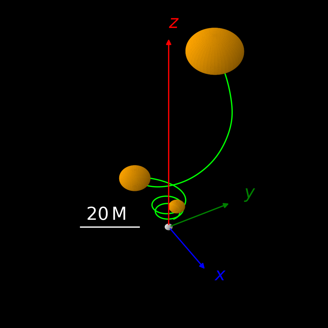
Note that as the plasmoid leaves the central regions near the black hole and moves outwards in regions of decreasing density and pressure, it expands because of the increased internal energy and accelerates moving outwards. Assuming the plasmoid is quasi-spherical and hence has a limited extent in the azimuthal direction, the reconstructed plasmoid trajectory is obtained after integrating in time the velocity of its core, including the azimuthal component. This is shown in Fig. 10 where it is seen that the expanding plasmoid performs orbits from its formation close to the black hole at to the end of the track at . When scaled to the mass of Sgr A*, the orbital period of the helical trajectory ranges from to . It is an intriguing possibility to consider the orbiting plasmoid discussed here in the context of the astrometrically resolved flares recently observed by the GRAVITY collaboration (Abuter et al., 2018).
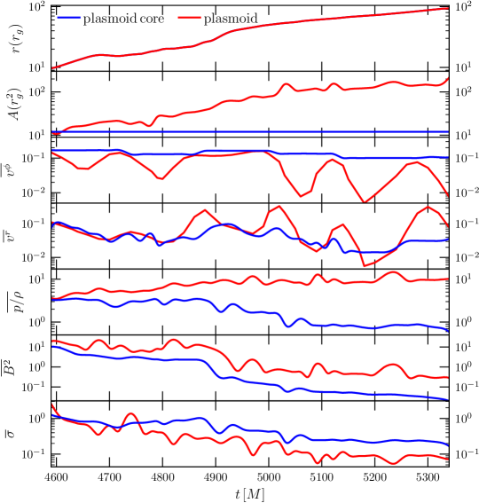
A more quantitative assessment of the dynamical and thermodynamical evolution of the plasmoid is presented in Fig. 11, where we show several quantities relative to the plasmoid, either when spatially averaged or when referring to the core of the plasmoid, which we define as a circle of radius centered at the plasmoid’s center. In the upper panel of Fig. 11, we monitor the distance of the plasmoid from the black hole, whereas in the second row we show the evolution of the size of the plasmoid by measuring its surface area. Note that the plasmoid’s size increases continuously, reaching a size of after from its formation. Through the third and fourth row of Fig. 11, where we plot the azimuthal component and the radial velocity, we can reconstruct the plasmoid’s kinematics. Note that the average velocity of the plasmoid fluctuates considerably (red line in Fig. 11) and is quite distinct from the evolution of the average velocity of the core of plasmoid (blue line). More specifically, while the latter remains almost constant at a velocity of , the former varies quasi-periodically, oscillating between and .
Another important quantity characterising the properties of the plasmoid is its temperature, which we measure through the ratio . Interestingly, the core of the plasmoid cools significantly, namely, by almost an order of magnitude over the time the plasmoid is followed, essentially because of the decrease in pressure as it moves outwards. On the other hand, the whole plasmoid’s temperature increases steadily over time as a result of the interaction of the plasmoid with the surrounding matter and its dynamics. Finally, the average magnetic-field strength (sixth row) is decreasing, together with the magnetization (seventh row).
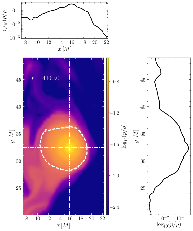
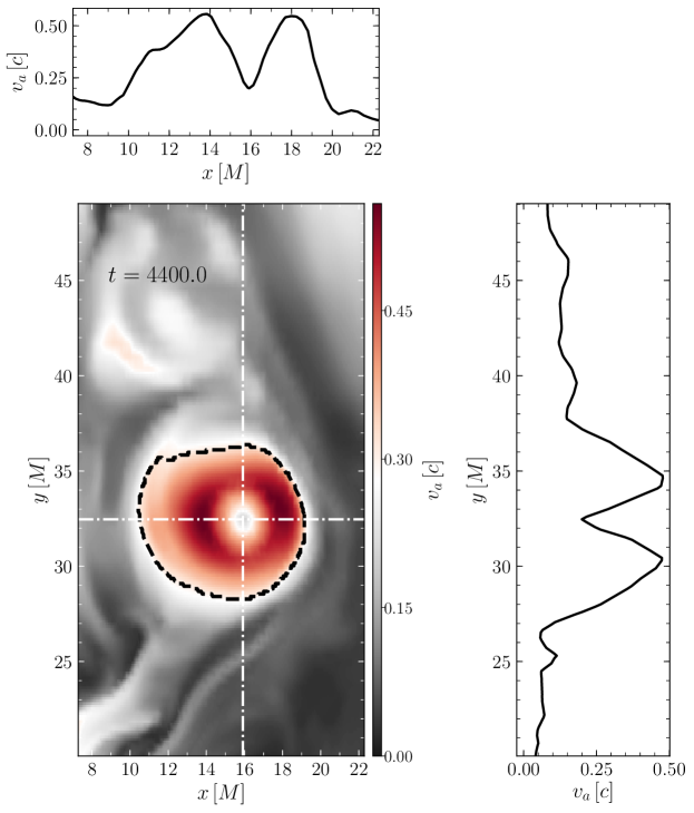
Any single plasmoid that can be isolated and tracked, can then be studied in detail in all of its interesting quantities. As an example, we report in Fig. 12 one-dimensional cuts for a single plasmoid and in terms of the quantities and . The two subplots show the vertical and horizontal cuts through the center of the plasmoid. In the right panel of Fig. 12, the shape of the plasmoid (which remains unchanged when shown in terms of the magnetization) provides a representative example about the use of the second method for the detection of a plasmoid, in which we first determine the center of the plasmoid as a local minimum and then detect the boundary of the plasmoid by finding first the local maxima. At the same time, the same panel shows how falls off by two orders of magnitude when reaching the outer layers of the plasmoid. A similar structure is evident also in the Bernoulli constant , as is seen in the right panel Fig. 12.
4 Conclusions
We have performed a series of GRMHD simulations of accreting tori onto a rotating black hole employing different topologies for the initial magnetic field. One goal of these simulations was to illustrate and confirm that when employing an initial magnetic-field configuration that does not consist of the standard single poloidal-field loop, a stationary jet configuration does not form.
We have observed that the evolution of toris with initial magnetic loops with alternating polarity (multi-loop initial topology; Models C and D) differs dramatically from the dynamics of small scale loops of the same polarity (Model B). Same-polarity loops quickly reconnect to form a large loop with resulting flow similar to the single loop setup (Model A). On the other hand, opposite-polarity loops preserve their small coherence length, giving rise to copious plasmoids in the ensuing turbulent evolution. These magnetic fields with small coherence lengths are advected to the black hole and give rise to fluctuating jets of low average power ( times the jet power with tori having the same polarity) but large variability. On rare occasions, the fluctuating jet power can reach or exceed the typical jet power in the same polarity cases which amounts to of the accretion power in our Model A scenario. In addition, tori having a multi-loop initial topology produce an accretion flow that does not produce a stationary magnetized jet, but a series of regions of poloidal and toroidal magnetic fields with alternating polarities. At the boundaries of these regions, reconnection can take place and generate plasmoids with large magnetization.
Most of the plasmoids are either accreted to the black hole or remain in the high-density torus. However, those plasmoids generated in reconnection layers with relatively high magnetization, i.e., , are outward moving in the funnel region and gravitationally unbound.
While the appearance of plasmoids generated during the simulations is rather straighforward, their automatic detection and characterization is far more complex. To handle this processs we have devised two different methods to detect the plasmoids at any given time during the simulation. In essence, we detect the center of a plasmoid in terms of a “blob-detector” algorithm and then define the boundary of the plasmoid either as an edge (usually in terms of the Bernoulli constant or of the temperature ) or as local maxima (usually in terms of the Alfvèn velocity or the magnetization ). In this manner, plasmoids can be tracked in the most interesting regions of the domain and their dynamics studied individually.
Recent observations of flaring activity and variability from AGNs hint that very rapid particle acceleration is required and that the emission region is relatively compact, few Schwarzschild radii (Levinson, 2007; Begelman et al., 2008; Ghisellini & Tavecchio, 2008; Giannios et al., 2009). Magnetic reconnection in the vicinity of a black hole can provide both rapid particle acceleration and a compact emission region. Our simulations have therefore shown that the models with an initial (opposite polarity) multi-loop magnetic geometry exhibit an intense variability in the power lost via outflows. This is ultimately the result of the accretion process, which forces small scale loops to be transported near the black hole – in particular in the polar regions, where the magnetization is larger – and reconnect. The consequent release of magnetic energy in these plasma regions and the formation of plasmoid are then responsible for the intense variability in the emitted power. Hence, the generic behaviour found in these simulations can have implications on the observed variability of AGNs, even when they are experiencing low accretion rates, such as Sgr A∗.
Furthermore, the episodic reconnection that occurs close to the black hole produces plasmoid chains filled with relativistic particles. These plasmoids can represent an additional source of variability in the vicinity of the black hole. The production of large plasmoid chains also has a considerable impact on the emitted power of the outflow, which is observed to increases of more than two orders of magnitude at times (Ponti et al., 2017; Do et al., 2019). Finally, the evidence that these plasmoids have nonzero angular momentum and hence an orbital motion, makes them potentially related to the observations of orbiting material recently made near the galactic center (Abuter et al., 2018).
Despite the absence of physical resistivity in our mathematical formulation of the GRMHD equations, magnetic reconnection is produced during the simulations and is generated entirely by the finite numerical resolution. As a result, the numerical methods employed in this study could be considered as inadequate for a detailed description of the generation and evolution of energetic plasmoids. However, as shown through the comparison of simulations carried out at different and increasing resolutions (see Appendix C), the main qualitative features discussed here are robustly produced across all different resolutions. This provides convincing evidence that the basic resistive features discussed here are qualitatively correct and that reconnection occurring in magnetically dominated regions can produce energized plasmoids that are outgoing and gravitationally unbound.
There are several and natural extensions of this work. First, by carrying out a more detailed investigation of the statistical properties of the plasmoids. This involves not only the processes leading to their formation, but also to the factors that determine their evolution and emission. Second, and more importantly, by investigating the phenomenology discussed here when employing a fully resistive formulation of the GRMHD equations (see, e.g., Palenzuela et al. 2009; Dionysopoulou et al. 2013; Ripperda et al. 2019a), so as to assess the properties of the plasmoids when different and resolution-independent values of the physical resistivity are considered. A complete description of the MHD properties of the plasmoids will allow the study of particle acceleration and radiation signatures due to the plasmoid evolution in such a turbulent environment around black holes (Bacchini et al., 2019).
Acknowledgements
AN is supported in part via an Alexander von Humboldt Fellowship. Additional support comes in part from HGS-HIRe for FAIR, the LOEWE-Program in HIC for FAIR, “PHAROS”, COST Action CA16214, the ERC Synergy Grant “BlackHoleCam: Imaging the Event Horizon of Black Holes” (Grant No. 610058). The simulations were performed on SuperMUC at LRZ in Garching, on the GOETHE-HLR cluster at CSC in Frankfurt, and on the HazelHen cluster at HLRS in Stuttgart.
References
- Abuter et al. (2018) Abuter R., et al., 2018, Astron. Astrophys., 615, L15
- Aharonian et al. (2007) Aharonian F., et al., 2007, Astron. Astrophys., 470, 475
- Albert et al. (2007) Albert J., et al., 2007, Astrophys. J., 663, 125
- Bacchini et al. (2019) Bacchini F., Ripperda B., Porth O., Sironi L., 2019, Astrophys. J., Supp., 240, 40
- Balbus & Hawley (1991) Balbus S. A., Hawley J. F., 1991, Astrophys. J., 376, 214
- Ball et al. (2018a) Ball D., Özel F., Psaltis D., Chan C.-K., Sironi L., 2018a, Astrophys. J., 853, 184
- Ball et al. (2018b) Ball D., Sironi L., Özel F., 2018b, Astrophys. J., 862, 80
- Bay et al. (2006) Bay H., Tuytelaars T., Van Gool L., 2006, in Leonardis A., Bischof H., Pinz A., eds, Computer Vision – ECCV 2006. Springer Berlin Heidelberg, Berlin, Heidelberg, pp 404–417
- Beckwith et al. (2008) Beckwith K., Hawley J. F., Krolik J. H., 2008, Astrophys. J., 678, 1180
- Beckwith et al. (2009) Beckwith K., Hawley J. F., Krolik J. H., 2009, Astrophys. J., 707, 428
- Begelman et al. (2008) Begelman M. C., Fabian A. C., Rees M. J., 2008, Mon. Not. R. Astron. Soc., 384, L19
- Blandford & Payne (1982) Blandford R. D., Payne D. G., 1982, Mon. Not. R. Astron. Soc., 199, 883
- Blandford & Znajek (1977) Blandford R. D., Znajek R. L., 1977, Mon. Not. R. Astron. Soc., 179, 433
- Boehle et al. (2016) Boehle A., et al., 2016, Astrophys. J., 830, 17
- Bovard et al. (2017) Bovard L., Martin D., Guercilena F., Arcones A., Rezzolla L., Korobkin O., 2017, Phys. Rev. D, 96, 124005
- Canny (1986) Canny J., 1986, IEEE Transactions on Pattern Analysis and Machine Intelligence, PAMI-8, 679
- Chael et al. (2018) Chael A., Rowan M., Narayan R., Johnson M., Sironi L., 2018, Mon. Not. R. Astron. Soc., 478, 5209
- Christie et al. (2019) Christie I. M., Petropoulou M., Sironi L., Giannios D., 2019, Mon. Not. R. Astron. Soc., 482, 65
- Contopoulos & Kazanas (1998) Contopoulos I., Kazanas D., 1998, Astrophys. J., 508, 859
- Contopoulos et al. (2015) Contopoulos I., Nathanail A., Katsanikas M., 2015, Astrophys. J., 805, 105
- Contopoulos et al. (2018) Contopoulos I., Nathanail A., Sa̧dowski A., Kazanas D., Narayan R., 2018, Mon. Not. R. Astron. Soc., 473, 721
- Cowling (1933) Cowling T. G., 1933, Mon. Not. R. Astron. Soc., 94, 39
- De Villiers et al. (2003) De Villiers J.-P., Hawley J. F., Krolik J. H., 2003, Astrophys. J., 599, 1238
- De Villiers et al. (2005) De Villiers J.-P., Hawley J. F., Krolik J. H., Hirose S., 2005, Astrophys. J., 620, 878
- Del Zanna et al. (2007) Del Zanna L., Zanotti O., Bucciantini N., Londrillo P., 2007, Astron. Astrophys., 473, 11
- Dionysopoulou et al. (2013) Dionysopoulou K., Alic D., Palenzuela C., Rezzolla L., Giacomazzo B., 2013, Phys. Rev. D, 88, 044020
- Dionysopoulou et al. (2015) Dionysopoulou K., Alic D., Rezzolla L., 2015, Phys. Rev. D, 92, 084064
- Do et al. (2019) Do T., et al., 2019, arXiv e-prints, p. arXiv:1908.01777
- Event Horizon Telescope Collaboration et al. (2019) Event Horizon Telescope Collaboration et al., 2019, Astrophys. J. Lett., 875, L5
- Fermo et al. (2010) Fermo R. L., Drake J. F., Swisdak M., 2010, Physics of Plasmas, 17, 010702
- Fishbone & Moncrief (1976) Fishbone L. G., Moncrief V., 1976, Astrophys. J., 207, 962
- Fleming et al. (2000) Fleming T. P., Stone J. M., Hawley J. F., 2000, Astrophys. J, 530, 464
- Gammie et al. (2004) Gammie C. F., Shapiro S. L., McKinney J. C., 2004, Astrophys. J., 602, 312
- Ghisellini & Tavecchio (2008) Ghisellini G., Tavecchio F., 2008, Mon. Not. R. Astron. Soc., 386, L28
- Giannios (2013) Giannios D., 2013, Mon. Not. R. Astron. Soc., 431, 355
- Giannios & Sironi (2013) Giannios D., Sironi L., 2013, Mon. Not. R. Astron. Soc., 433, L25
- Giannios et al. (2009) Giannios D., Uzdensky D. A., Begelman M. C., 2009, Mon. Not. R. Astron. Soc., 395, L29
- Guo et al. (2014) Guo Y.-J., Lai X.-Y., Xu R.-X., 2014, Chinese Physics C, 38, 055101
- Guo et al. (2015) Guo F., Liu Y.-H., Daughton W., Li H., 2015, Astrophys. J., 806, 167
- Haggard et al. (2019) Haggard D., et al., 2019, arXiv e-prints, p. arXiv:1908.01781
- Harutyunyan et al. (2018) Harutyunyan A., Nathanail A., Rezzolla L., Sedrakian A., 2018, preprint, (arXiv:1803.09215)
- Huang & Bhattacharjee (2012) Huang Y.-M., Bhattacharjee A., 2012, Phys. Rev. Lett., 109, 265002
- Igumenshchev et al. (2003) Igumenshchev I. V., Narayan R., Abramowicz M. A., 2003, Astrophys. J., 592, 1042
- Kadowaki et al. (2018) Kadowaki L. H. S., De Gouveia Dal Pino E. M., Stone J. M., 2018, Astrophys. J., 864, 52
- Kagan et al. (2015) Kagan D., Sironi L., Cerutti B., Giannios D., 2015, Space Science Reviews, 191, 545
- Kagan et al. (2018) Kagan D., Nakar E., Piran T., 2018, Mon. Not. R. Astron. Soc., 476, 3902
- Komissarov & Barkov (2009) Komissarov S. S., Barkov M. V., 2009, Mon. Not. R. Astron. Soc., 397, 1153
- Komissarov et al. (2009) Komissarov S. S., Vlahakis N., Königl A., Barkov M. V., 2009, Mon. Not. R. Astron. Soc., 394, 1182
- Levinson (2007) Levinson A., 2007, Astrophys. J. Letters, 671, L29
- Li et al. (2017a) Li Y.-P., Yuan F., Wang Q. D., 2017a, Mon. Not. R. Astron. Soc., 468, 2552
- Li et al. (2017b) Li X., Guo F., Li H., Li G., 2017b, Astrophys. J., 843, 21
- Liska et al. (2018) Liska M. T. P., Tchekhovskoy A., Quataert E., 2018, arXiv e-prints, p. arXiv:1809.04608
- Loureiro et al. (2007) Loureiro N. F., Schekochihin A. A., Cowley S. C., 2007, Physics of Plasmas, 14, 100703
- Loureiro et al. (2012) Loureiro N. F., Samtaney R., Schekochihin A. A., Uzdensky D. A., 2012, Physics of Plasmas, 19, 042303
- Lyubarsky (2009) Lyubarsky Y., 2009, Astrophys. J., 698, 1570
- McKinney (2006) McKinney J. C., 2006, Mon. Not. R. Astron. Soc., 368, L30
- McKinney & Blandford (2009) McKinney J. C., Blandford R. D., 2009, Mon. Not. R. Astron. Soc., 394, L126
- McKinney & Gammie (2004) McKinney J. C., Gammie C. F., 2004, Astrophys. J, 611, 977
- McKinney et al. (2012) McKinney J. C., Tchekhovskoy A., Blandford R. D., 2012, Mon. Not. R. Astron. Soc., 423, 3083
- Mizuno et al. (2018) Mizuno Y., et al., 2018, Nature Astronomy,
- Narayan et al. (2003) Narayan R., Igumenshchev I. V., Abramowicz M. A., 2003, Publications of the ASJ, 55, L69
- Narayan et al. (2012) Narayan R., SÄ dowski A., Penna R. F., Kulkarni A. K., 2012, Mon. Not. R. Astron. Soc., 426, 3241
- Nathanail et al. (2019) Nathanail A., Porth O., Rezzolla L., 2019, Astrophys. J. Lett, 870, L20
- Obergaulinger et al. (2009) Obergaulinger M., Cerdá-Durán P., Müller E., Aloy M. A., 2009, Astron. Astrophys., 498, 241
- Olivares et al. (2019) Olivares H., Porth O., Davelaar J., Most E. R., Fromm C. M., Mizuno Y., Younsi Z., Rezzolla L., 2019, arXiv e-prints, p. arXiv:1906.10795
- Palenzuela et al. (2009) Palenzuela C., Lehner L., Reula O., Rezzolla L., 2009, Mon. Not. R. Astron. Soc., 394, 1727
- Parfrey et al. (2015) Parfrey K., Giannios D., Beloborodov A. M., 2015, Mon. Not. R. Astron. Soc., 446, L61
- Parker (1966) Parker E. N., 1966, Astrophys. J., 145, 811
- Petropoulou et al. (2016) Petropoulou M., Giannios D., Sironi L., 2016, Mon. Not. R. Astron. Soc., 462, 3325
- Petropoulou et al. (2018) Petropoulou M., Christie I. M., Sironi L., Giannios D., 2018, Mon. Not. R. Astron. Soc., 475, 3797
- Petropoulou et al. (2019) Petropoulou M., Sironi L., Spitkovsky A., Giannios D., 2019, Astrophys. J., 880, 37
- Ponti et al. (2017) Ponti G., et al., 2017, Mon. Not. R. Astron. Soc., 468, 2447
- Porth et al. (2017) Porth O., Olivares H., Mizuno Y., Younsi Z., Rezzolla L., Moscibrodzka M., Falcke H., Kramer M., 2017, Computational Astrophysics and Cosmology, 4, 1
- Porth et al. (2019) Porth O., et al., 2019, arXiv e-prints, p. arXiv:1904.04923
- Rezzolla & Zanotti (2013) Rezzolla L., Zanotti O., 2013, Relativistic Hydrodynamics. Oxford University Press, Oxford, UK, doi:10.1093/acprof:oso/9780198528906.001.0001
- Rezzolla et al. (2011) Rezzolla L., Giacomazzo B., Baiotti L., Granot J., Kouveliotou C., Aloy M. A., 2011, Astrophys. J. Letters, 732, L6
- Ripperda et al. (2019a) Ripperda B., et al., 2019a, ApJS, 244, 10
- Ripperda et al. (2019b) Ripperda B., Porth O., Sironi L., Keppens R., 2019b, Mon. Not. R. Astron. Soc., 485, 299
- Sano et al. (2004) Sano T., Inutsuka S.-i., Turner N. J., Stone J. M., 2004, Astrophys. J., 605, 321
- Sa̧dowski et al. (2015) Sa̧dowski A., Narayan R., Tchekhovskoy A., Abarca D., Zhu Y., McKinney J. C., 2015, Mon. Not. R. Astron. Soc., 447, 49
- Siegel et al. (2013) Siegel D. M., Ciolfi R., Harte A. I., Rezzolla L., 2013, Phys. Rev. D R, 87, 121302
- Sironi & Spitkovsky (2014) Sironi L., Spitkovsky A., 2014, Astrophys. J.l, 783, L21
- Sironi et al. (2016) Sironi L., Giannios D., Petropoulou M., 2016, Mon. Not. R. Astron. Soc., 462, 48
- Takahashi (2008) Takahashi R., 2008, Mon. Not. R. Astron. Soc., 383, 1155
- Takamoto (2013) Takamoto M., 2013, Astrophys. J., 775, 50
- Tchekhovskoy et al. (2009) Tchekhovskoy A., McKinney J. C., Narayan R., 2009, Astrophys. J., 699, 1789
- Tchekhovskoy et al. (2011) Tchekhovskoy A., Narayan R., McKinney J. C., 2011, Mon. Not. R. Astron. Soc., 418, L79
- Uzdensky et al. (2010) Uzdensky D. A., Loureiro N. F., Schekochihin A. A., 2010, Phys. Rev. Lett., 105, 235002
- Werner et al. (2016) Werner G. R., Uzdensky D. A., Cerutti B., Nalewajko K., Begelman M. C., 2016, Astrophys. J. Let., 816, L8
- Younsi & Wu (2015) Younsi Z., Wu K., 2015, Mon. Not. R. Astron. Soc., 454, 3283
- Yuan et al. (2009) Yuan F., Lin J., Wu K., Ho L. C., 2009, Mon. Not. R. Astron. Soc., 395, 2183
- Zhang & Shu (2011) Zhang X., Shu C.-W., 2011, Proceedings of the Royal Society A: Mathematical, Physical and Engineering Sciences, 467, 2752
- Zhang et al. (2018) Zhang H., Li X., Guo F., Giannios D., 2018, Astrophys. J. Lett., 862, L25
- di Matteo (1998) di Matteo T., 1998, Mon. Not. R. Astron. Soc., 299, L15
- van der Walt et al. (2014) van der Walt S., et al., 2014, PeerJ, 2, e453
Appendix A Plasmoid Tracking
In this Appendix we discuss in more detail the methods we use to detect and track plasmoids and follow their evolution. The study of their dynamics, expansion and cooling, represents a first step towards modeling flares emerging from the vicinity of the black hole in AGNs.
More specifically, in tracking the plasmoid we have made use of the python package scikit-image (van der Walt et al., 2014). In order to identify blob structures, we use the difference of Gaussians method (Bay et al., 2006). In this approach, the data-image is successively convolved with a Gaussian kernel with increasing standard deviation (essentially blurred). The difference between the two new images is used to identify higher-intensity regions against a lower-intensity background. In this first step, the identification is done through the Bernoulli constant , since it has turned out to yield more robust results. After a plasmoid is identified, the coordinates of its center are determined. Usually, this comes with an estimation of the radius of the plasmoid. However, most of the plasmoids during the simulation are not completely spherical, so the radius alone cannot define the boundary of the plasmoid. In most cases, the plasmoid-structure has several irregularities, so that we divide the domain into squares whose number is proportional to the number of plasmoids that have been found. For every plasmoid, we cut a neighbourhood around it that includes the radius estimation from the previous step. In this way, in every square there is only one plasmoid, whose boundary is found using the Canny edge-detector algorithm (Canny, 1986). The algorithm is applied In the case when the plasmoid has an irregular boundary, we are left with a curve which is not closed or with two or more smaller curves. In this case, then we continue by finding the convex hull of the resulting curve or curves from the previous step. In all tests, at this point the boundary of the plasmoid was adequately described.
In the second method used, after detecting the plasmoid with the same way as discussed before, we then cut the domain into squares that include the center of the plasmoid and its radius estimation. Next, we focus on the magnetization parameter (or the Alfvèn speed), which normally exhibits a local minimum at the center of the plasmoid. We then find around the center the local maxima and in that way define the boundary of the plasmoid. Measuring in such a way the distance between the center of the plasmoid and the local maxima, we can define the boundary in terms of this distance. Finally, as a validation check, we calculate the convex hull of these contours to verify that the center of the plasmoid is indeed surrounded by the configuration we have found.
In the three panels of Fig. 9 we have presented the tracking of a single plasmoid in terms of the Bernoulli constant, of the toroidal magnetic field, and of the magnetization. In all snapshots except one, the boundary is found after applying the Canny-edge detector algorithm. However, in the snapshot with time , the plasmoid boundary is not easily identified, which make it difficult to define a closed boundary from the edges; in this case, the calculation of convex hull was used. As a result, that for this specific snapshot, the shape of the boundary of the plasmoid resembles a polygon.
Appendix B On the sustainability of MRI turbulence in the torus
We here provide evidence that the MRI is properly resolved throughout the simulations by focussing only in the runs with the multi-loop magnetic field structure with the alternating polarity, i.e., Model D at the three resolutions in Table 1. A well-resolved MRI is essential, since it provides a sustained source of turbulence and – in turn – a quasi-stationary accretion process with an accretion rate that is roughly constant in time.
As customary in these cases, we evaluate the so-called “quality factor” in terms of the ration between the grid spacing in a given direction , (e.g., the -direction) and the wavelength of the fastest growing MRI mode in that direction (i.e., ), where both quantities are evaluated in the tetrad basis of the fluid frame (see Takahashi 2008; Siegel et al. 2013; Porth et al. 2019, for details)
| (10) |
where
| (11) |
is the angular velocity of the fluid and the corresponding grid resolution is .
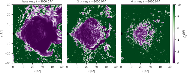
The spatial distributions of the quality factor for three different resolutions , , and the base resolution are shown in the various panels of Fig. 13 at time . The left and middle panels, which refer to low and middle resolutions, show that in these cases and at the time considered the turbulence has started to decay and indeed the MRI is under-resolved in the torus, as shown by the fact that it appears as mostly filled in purple. On the other hand, the high-resolution run (right panel in Fig. 13) shows that the MRI is in this case well resolved, matching the expectation that with at least six cells covering , the MRI is effectively resolved (Sano et al., 2004). Furthermore, at this resolution, the accretion rate maintains a rather constant value till time , which is much longer than the typical timescale investigated here (i.e., ).
Appendix C Dependence on resolution and numerical resistivity
Although resistivity plays a very important role in astrophysical scenarios in general and in accretion disks in particular, its precise value and dependence on the properties of the plasma (e.g., temperature and density) is still poorly known (Fleming et al., 2000; Harutyunyan et al., 2018). In this Appendix we discuss the dependence of our results on resolution, since in our simulations – which solve the equations of ideal-MHD – the resistivity is purely numerical. At the same time, we recall that previous work has explored the effect of resistivity on the formation and growth rate of plasmoids and at which specific values the “plasmoid regime” – i.e., the regime where plasmoid growth is exponentially rapid – takes place (Ripperda et al., 2019b). Furthermore, it has been argued that in ideal-MHD, numerical resistivity yields results comparable with the analytic expectations (Obergaulinger et al., 2009).
It is important to note that plasmoids in Model D exist at all resolutions that we have tested, which are relatively high for GRMHD simulations (Porth et al., 2019; Event Horizon Telescope Collaboration et al., 2019).
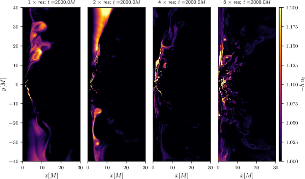
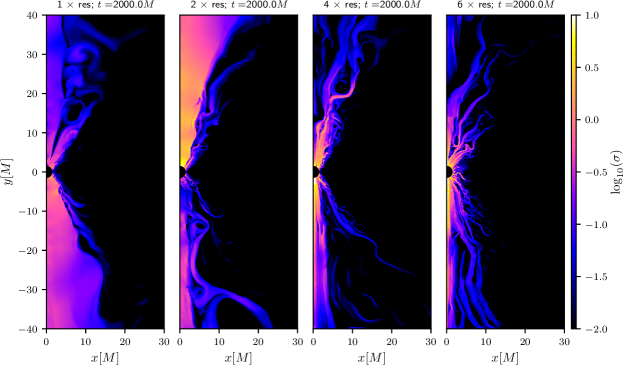
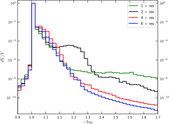
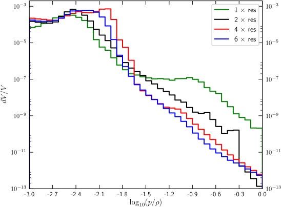
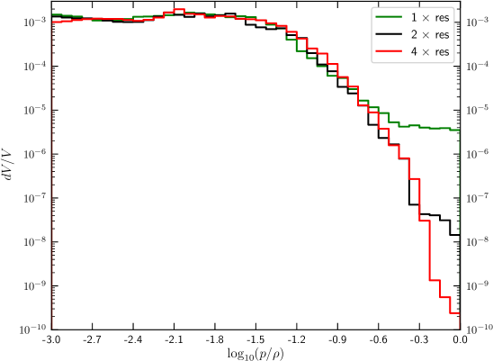
In the lower panels of Fig. 14 we plot the magnetization parameter for the all four resolution for Model D at a time . As expected, from the previous discussion, the first two runs show a much different distribution of magnetization. In the two high resolution runs the magnetization has a very similar structure. This structure seems to be affected by the plasmoid production and the actual size of the plasmoids. At later times a difference in magnetization is also evident for the high resolution runs. However, due to the turbulent nature of the processes leading to reconnection and thus to the production of plasmoids, a single snapshot at a given time cannot fully illustrate and capture any differences in magnetization due to resolution.
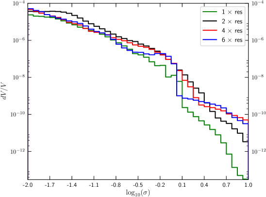
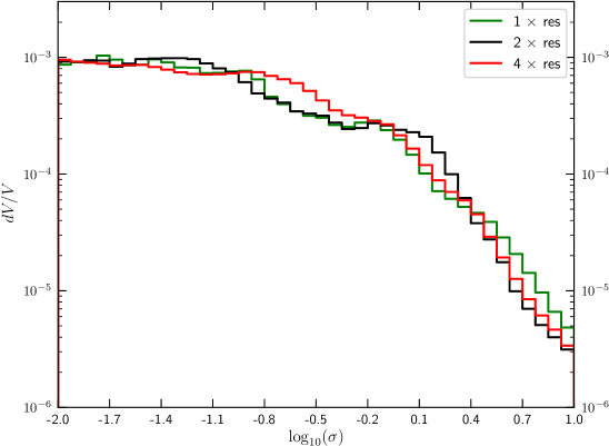
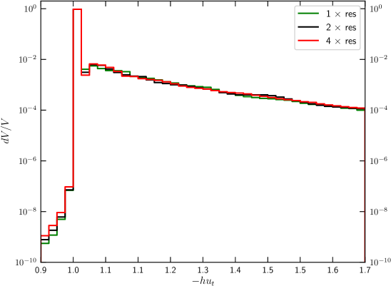
For a quantitative comparison of the whole evolution of magnetization and the effective heating of the plasmoids, we have computed the distribution functions of the volume fraction as a function of those quantities that are more sensitive to changes in resolution, namely, and . Figure 15 reports these distributions for Model D, over the timeframe , and shows that for the two runs with lower resolution, the distribution of the volume fractions are very different for all quantities. This is not the case for the two runs with higher resolution, where both results agree well in highly magnetized regions. This shows that the resolutions used are sufficient, not only for resolving the MRI, but also for a robust description of the plasmoid production and evolution. Similar distributions are shown in Fig. 16 for Model A, where it is possible to appreciate that the plasma is well described already with the base resolution and that tori with single nested loops generically produce flows with larger magnetization, stronger outflows and higher internal energies.