USTC-ICTS/PCFT-20-03

Perturbative string theory from Newtonian limit of string geometry theory

Matsuo Sato^∗ and Yuji Sugimoto^†,‡

^∗Graduate School of Science and Technology, Hirosaki University
Bunkyo-cho 3, Hirosaki, Aomori 036-8561, Japan

^†Interdisciplinary Center for Theoretical Study, University of Science and Technology of China, Hefei, Anhui 230026, China

^‡Peng Huanwu Center for Fundamental Theory, Hefei, Anhui 230026, China

String geometry theory is one of the candidates of the non-perturbative formulation of string theory. In [1], the perturbative string theory is reproduced from a string geometry model coupled with a $u(1)$ gauge field on string manifolds. In this paper, we generalize this result and we show that the perturbative string theory is reproduced from any string geometry model by taking a Newtonian limit.

1 Introduction

String geometry theory is one of the candidates of non-perturbative formulation of string theory [1]. Especially, from a sting geometry model coupled with a $u(1)$ gauge field, one can derive the all-order perturbative scattering amplitudes that possess the super moduli in IIA, IIB and SO(32) I superstring theories, by considering fluctuations around fixed perturbative IIA, IIB and SO(32) I vacuum background, respectively as in [1].

Then, a natural question arises as to whether a perturbative string theory can be reproduced if a string geometry model couples with other fields. Is the $u(1)$ gauge field special? Or, can it be reproduced from any string geometry model?

To answer this question, let us reconsider how the perturbative string theory is reproduced from the string geometry model coupled with the $u(1)$ gauge field. In this case, it is derived from fluctuations around a background including a potential that satisfies the harmonic equation on the flat background. A low-velocity limit is also taken. These facts indicate Newtonian limit. Then, we examine all the string geometry models by taking a Newtonian limit in this paper.

The organization of the paper is as follows. In section 2, we shortly review the framework of string geometry theory. In section 3, we show that a Newtonian limit of any string geometry model reproduces the perturbative string theory. In section 4, we conclude and discuss our results. In appendix A, we clarify the relation between the results of this paper and of the previous paper in case of coupling with a $u(1)$ gauge field on string manifolds. In appendix B, we display an explicit form of the Lagrangian up to the second order in the fluctuations.

2 String geometry theory

In this paper, we discuss only the closed bosonic sector of string geometry theory [1]. One can generalize the result in this paper to the full string geometry theory in the same way as in [1]. The closed bosonic sector is described by a partition function

$$Z=\int\mathcal{D}G\mathcal{D}Ce^{-S},$$ (2.1)

where the action in general is given by

$$S=\frac{1}{G_{N}}\int\mathcal{D}h\mathcal{D}X(\bar{\tau})\mathcal{D}\bar{\tau}\sqrt{G}(-R+(\mbox{tensor and higher derivative terms})),$$ (2.2)

where $G_{N}$ is a constant. The action consists of a metric $G_{IJ}$ and tensor fields $C$ including scalar fields defined on an infinite dimensional manifold, so-called string manifold. String manifold is constructed by patching open sets in string model space $E$, whose definition is summarized as follows. First, a global time $\bar{\tau}$ is defined canonically and uniquely on a Riemann surface $\bar{\Sigma}$ by the real part of the integral of an Abelian differential uniquely defined on $\bar{\Sigma}$ [3, 4]. We restrict $\bar{\Sigma}$ to a $\bar{\tau}$ constant line and obtain $\bar{\Sigma}|_{\bar{\tau}}$. An embedding of $\bar{\Sigma}|_{\bar{\tau}}$ to $\mathbb{R}^{d}$ represents a many-body state of strings in $\mathbb{R}^{d}$, and is parametrized by coordinates $(\bar{h},X(\bar{\tau}),\bar{\tau})$ where $\bar{h}$ is a metric on $\bar{\Sigma}$ and $X(\bar{\tau})$ is a map from $\bar{\Sigma}|_{\bar{\tau}}$ to $\mathbb{R}^{d}$. String model space $E$ is defined by the collection of the string states by considering all the $\bar{\Sigma}$, all the values of $\bar{\tau}$, and all the $X(\bar{\tau})$. How near the two string states is defined by how near the values of $\bar{\tau}$ and how near $X(\bar{\tau})$. By this definition, arbitrary two string states on a connected Riemann surface in $E$ are connected continuously. Thus, there is an one-to-one correspondence between a Riemann surface in $\mathbb{R}^{d}$ and a curve parametrized by $\bar{\tau}$ from $\bar{\tau}=-\infty$ to $\bar{\tau}=\infty$ on $E$. That is, curves that represent asymptotic processes on $E$ reproduce the right moduli space of the Riemann surfaces in $\mathbb{R}^{d}$. Therefore, a string geometry model possesses all-order information of string theory.

We use the Einstein notation for the index $I$, where $I=\{d,(\mu\bar{\sigma})\}$. The cotangent space is spanned by $dX^{d}:=d\bar{\tau}$ and $dX^{(\mu\bar{\sigma})}:=dX^{\mu}\left(\bar{\sigma},\bar{\tau}\right)$ for $\mu=0,1,\dots,d-1$, while $d\bar{h}_{mn}$ with $m,n=\bar{\tau},\bar{\sigma}$ cannot be a part of the basis because $\bar{h}_{mn}$ is treated as a discrete valuable in the string topology. The summation over $\bar{\sigma}$ is defined by $\int d\bar{\sigma}\bar{e}(\bar{\sigma},\bar{\tau})$, where $\bar{e}:=\sqrt{\bar{h}_{\bar{\sigma}\bar{\sigma}}}$. This summation is transformed as a scalar under $\bar{\tau}\mapsto\bar{\tau}^{\prime}(\bar{\tau},X(\bar{\tau}))$, and invariant under $\bar{\sigma}\mapsto\bar{\sigma}^{\prime}(\bar{\sigma})$.

From these definitions, we can write down the general form of the metric of the string geometry as follows.

$$ds^{2} (\bar{h},X(\bar{\tau}),\bar{\tau})$$

$$= G_{dd}(\bar{h},X(\bar{\tau}),\bar{\tau})(d\bar{\tau})^{2}+2d\bar{\tau}\int d\bar{\sigma}\bar{e}(\bar{\sigma},\bar{\tau})\sum_{\mu}G_{d\;(\mu\bar{\sigma})}(\bar{h},X(\bar{\tau}),\bar{\tau})dX^{\mu}(\bar{\sigma},\bar{\tau})$$

$$+\int d\bar{\sigma}\bar{e}(\bar{\sigma},\bar{\tau})\int d\bar{\sigma}^{\prime}\bar{e}(\bar{\sigma}^{\prime},\bar{\tau})\sum_{\mu,\mu^{\prime}}G_{\;(\mu\bar{\sigma})\;(\mu^{\prime}\bar{\sigma}^{\prime})}(\bar{h},X(\bar{\tau}),\bar{\tau})dX^{\mu}(\bar{\sigma},\bar{\tau})dX^{\mu^{\prime}}(\bar{\sigma}^{\prime},\bar{\tau}).$$

In this way, string geometry theory is a field theory on a loop space. Thus, we can expect that the theory includes non-perturbative effects as string field theory.

3 Newtonian limit of string geometry theory

In this section, we show that a Newtonian limit of the string geometry model reproduces the perturbative string theory.

The Newtonian limit of string geometry theory is defined by (0) low-velocity limit under three conditions:

• weak gravity condition

• stationary condition for the background

• tensor-less condition.

First, we consider the Newtonian potential background around a flat background:

$$\bar{ds}^{2} = 2\lambda\bar{\rho}(\bar{h})(1+\alpha\phi(X(\bar{\tau})))(dX^{d})^{2}$$ (3.1)

$$+\int d\bar{\sigma}\bar{e}\int d\bar{\sigma}^{\prime}\bar{e}^{\prime}(1+\frac{1}{2-D}\alpha\phi(X(\bar{\tau})))\frac{\bar{e}^{3}(\bar{\sigma},\bar{\tau})}{\sqrt{\bar{h}(\bar{\sigma},\bar{\tau})}}\delta_{(\mu\bar{\sigma})(\mu^{\prime}\bar{\sigma}^{\prime})}dX^{(\mu\bar{\sigma})}dX^{(\mu^{\prime}\bar{\sigma}^{\prime})},$$

where $\lambda$ is a constant and $\bar{\rho}(\bar{h}):=\frac{1}{4\pi}\int d\bar{\sigma}\sqrt{\bar{h}}\bar{R}_{\bar{h}}$, where $\bar{R}_{\bar{h}}$ is the scalar curvature of $\bar{h}_{mn}$. The worldsheet metric $\bar{h}_{mn}$ behaves as a constant in the solution (3.1) to the equations of motion of (2.2) because they are differential equations with respect to $X^{\mu}(\bar{\tau})$ and $\bar{\tau}$. $D$ is a volume of the index $(\mu\bar{\sigma})$, $D:=\int d\bar{\sigma}\bar{e}\delta_{(\mu\bar{\sigma})(\mu\bar{\sigma})}=2\pi d\delta(0)$.

The equations of motion reduces to the Ricci flat condition,

$$R_{IJ}=0,$$ (3.2)

because the tensor and higher derivative terms are dropped off from the limit (0) and the condition (3). In addition, the Ricci flat condition reduces to a harmonic equation,

$$\int d\bar{\sigma}\bar{e}\frac{d}{dX^{(\mu\bar{\sigma})}}\frac{d}{dX^{(\mu\bar{\sigma})}}\phi(X(\bar{\tau}))=0,$$ (3.3)

because the condition (1) implies that $\phi\ll 1$ where $\phi$ remains up to the second order in the action and up to the first order in the equations of motion, and the condition (2) implies that $\frac{d}{d\bar{\tau}}\phi=0$.

$$\phi(X(\bar{\tau}))={\rm i}\int d\bar{\sigma}\epsilon_{\mu\nu}X^{\mu}(\bar{\tau})\partial_{\bar{\sigma}}X^{\nu}(\bar{\tau})$$ (3.4)

is a solution to the harmonic equation, where

$$\epsilon_{\mu\nu}=-\epsilon_{\nu\mu}=\begin{cases}1~{}\text{ for }(\mu,\nu)=(0,1),(2,3),(4,5),...,(d-2,d-1),\\ 0~{}\text{ for others}.\end{cases}$$ (3.5)

We should note that $\bar{h}_{mn}$, $X^{\mu}(\bar{\tau})$ and $\bar{\tau}$ are all independent, and thus $\frac{\partial}{\partial\bar{\tau}}$ is an explicit derivative on functions over the string manifolds, especially, $\frac{\partial}{\partial\bar{\tau}}\bar{h}_{mn}=0$ and $\frac{\partial}{\partial\bar{\tau}}X^{\mu}(\bar{\tau})=0$.

The dependence of $\bar{h}_{mn}$ on the background (3.1) is uniquely determined by the consistency of the quantum theory of the fluctuations around the background. Namely, a propagator of the fluctuations becomes to be the path-integral of the perturbative string on the flat background as we will see in the remaining part of this paper. The dependence is uniquely determined if one assumes that the theory has the two-dimensional diffeomorphism times Weyl invariance quantum mechanically. The symmetry will be broken if one chooses the other dependence. This mechanism corresponds to the fact that a background is restricted to satisfy the equations of motion of the gravity if one supposes the two-dimensional diffeomorphism times Weyl invariance quantum mechanically in the perturbative string theory.

Let us consider fluctuations around the background (3.1), $G_{IJ}=\bar{G}_{IJ}+\tilde{G}_{IJ}$. Because of the limit (0) and the condition (3), the action (2.2) up to the quadratic order is given by

$$S = \frac{1}{G_{N}}\int\mathcal{D}h\mathcal{D}X(\bar{\tau})\mathcal{D}\bar{\tau}\sqrt{\bar{G}}\Bigl{(}-\bar{R}-(\bar{R}^{IJ}-\frac{1}{2}\bar{G}^{IJ}\bar{R})\tilde{G}_{IJ}$$ (3.6)

$$+\frac{1}{4}\bar{\nabla}_{I}\tilde{G}_{JK}\bar{\nabla}^{I}\tilde{G}^{JK}-\frac{1}{4}\bar{\nabla}_{I}\tilde{G}\bar{\nabla}^{I}\tilde{G}+\frac{1}{2}\bar{\nabla}^{I}\tilde{G}_{IJ}\bar{\nabla}^{J}\tilde{G}-\frac{1}{2}\bar{\nabla}^{I}\tilde{G}_{IJ}\bar{\nabla}_{K}\tilde{G}^{JK}$$

$$+\frac{1}{4}\bar{R}(\tilde{G}_{IJ}\tilde{G}^{IJ}-\frac{1}{2}\tilde{G}^{2})-\frac{1}{2}\bar{R}^{I}_{\;\;J}\tilde{G}_{IL}\tilde{G}^{JL}+\frac{1}{2}\bar{R}^{IJ}\tilde{G}_{IJ}\tilde{G}-\frac{1}{2}\bar{R}^{IJKL}\tilde{G}_{IK}\tilde{G}_{JL}\Bigr{)},$$

where $\tilde{G}:=\bar{G}^{IJ}\tilde{G}_{IJ}$. In order to fix the diffeomorphism symmetry, we take the harmonic gauge. If we add the gauge fixing term

$$S_{fix}=\frac{1}{G_{N}}\int\mathcal{D}h\mathcal{D}X(\bar{\tau})\mathcal{D}\bar{\tau}\sqrt{\bar{G}}\frac{1}{2}\Bigl{(}\bar{\nabla}^{J}(\tilde{G}_{IJ}-\frac{1}{2}\bar{G}_{IJ}\tilde{G})\Bigr{)}^{2},$$ (3.7)

we obtain

$$S^{\prime}+S_{fix} =\frac{1}{G_{N}}\int\mathcal{D}h\mathcal{D}X(\bar{\tau})\mathcal{D}\bar{\tau}\sqrt{\bar{G}}\Bigl{(}-\bar{R}-(\bar{R}^{IJ}-\frac{1}{2}\bar{G}^{IJ}\bar{R})\tilde{G}_{IJ}$$

$$\qquad+\frac{1}{4}\bar{\nabla}_{I}\tilde{G}_{JK}\bar{\nabla}^{I}\tilde{G}^{JK}-\frac{1}{8}\bar{\nabla}_{I}\tilde{G}\bar{\nabla}^{I}\tilde{G}+\frac{1}{4}\bar{R}(\tilde{G}_{IJ}\tilde{G}^{IJ}-\frac{1}{2}\tilde{G}^{2})-\frac{1}{2}\bar{R}^{I}_{\;\;J}\tilde{G}_{IL}\tilde{G}^{JL}$$

$$\qquad+\frac{1}{2}\bar{R}^{IJ}\tilde{G}_{IJ}\tilde{G}-\frac{1}{2}\bar{R}^{IJKL}\tilde{G}_{IK}\tilde{G}_{JL}\Bigr{)}.$$ (3.8)

We normalize the fields as $\tilde{H}_{IJ}:=Z_{IJ}\tilde{G}_{IJ}$, where $Z_{IJ}:=G_{N}^{-\frac{1}{2}}\bar{G}^{\frac{1}{4}}(\bar{\alpha}_{I}\bar{\alpha}_{J})^{-\frac{1}{2}}$. $\bar{\alpha}_{I}$ represent the background metric as $\bar{G}_{IJ}=\bar{\alpha}_{I}\delta_{IJ}$, where $\bar{\alpha}_{d}=2\lambda\bar{\rho}$ and $\bar{\alpha}_{(\mu\bar{\sigma})}=\frac{\bar{e}^{3}}{\sqrt{\bar{h}}}$. By using (3.1), we obtain

$$S^{\prime}+S_{fix}= \int\mathcal{D}h\mathcal{D}X(\bar{\tau})\mathcal{D}\bar{\tau}\left(L_{0}+L_{1}+L_{2}\right),$$ (3.9)

where $L_{0,1,2}$ are the terms of order $\mathcal{O}(\tilde{H}_{IJ}^{0,1,2})$. The explicit form is given in Appendix B.

In order to take (0) the low-velocity limit, we perform a derivative expansion of $\tilde{G}_{IJ}$. We perform (1) weak gravity expansion and the derivative expansion

$$\tilde{H}_{IJ} \to\frac{1}{\alpha}\tilde{H}_{IJ}$$ (3.10a)

$$\partial_{K}\tilde{H}_{IJ} \to\partial_{K}\tilde{H}_{IJ}$$ (3.10b)

$$\partial_{K}\partial_{L}\tilde{H}_{IJ} \to\alpha\partial_{K}\partial_{L}\tilde{H}_{IJ}$$ (3.10c)

$$G_{N} \to\alpha^{4}G_{N}$$ (3.10d)

and take the Newtonian limit

$$\alpha\to 0,$$ (3.11)

where $\alpha$ is an arbitrary constant in the solution (3.1). We have also redefined $G_{N}$. Then, (3.8) with appropriate boundary conditions reduces to

$$S^{\prime}+S_{fix}\to\int\mathcal{D}h\mathcal{D}X(\bar{\tau})\mathcal{D}\bar{\tau}\left(\tilde{L}_{0}+\tilde{L}_{1}+\tilde{L}_{2}\right),$$ (3.12)

where

$$\tilde{L}_{0}=\frac{1}{\alpha^{2}G_{N}}\left(\frac{3D^{2}-9D+10}{4(D-2)^{2}}\bar{\alpha}_{d}^{-2}\bar{\alpha}_{i}^{-1}\partial^{i}\phi\partial_{i}\phi\right),$$ (3.13)

$$\tilde{L}_{1}=\frac{1}{\alpha\sqrt{G_{N}}}\biggl{\{}-\frac{(D-1)(D-6)}{8(D-2)^{2}}\alpha^{2}\bar{\alpha}_{d}^{-2}\bar{\alpha}_{i}^{-1}\partial^{i}\phi\partial_{i}\phi\tilde{H}_{dd}+\frac{3(D-1)}{8(D-2)}\alpha^{2}\bar{\alpha}_{d}^{-2}\bar{\alpha}_{i}^{-1}\partial^{i}\phi\partial_{i}\phi\tilde{H}^{j}_{j}$$

$$\qquad\qquad\qquad+\biggl{(}-\frac{D-1}{4(D-2)}\alpha^{2}\bar{\alpha}_{d}^{-1}\partial_{i}\phi\partial_{j}\phi+\frac{D-1}{4(D-2)}\alpha^{2}\bar{\alpha}_{d}^{-1}\phi\partial_{i}\partial_{j}\phi\biggr{)}\bar{\alpha}_{d}^{-1}\bar{\alpha}_{i}^{-\frac{1}{2}}\bar{\alpha}_{j}^{-\frac{1}{2}}\tilde{H}^{ij}\biggr{\}},$$ (3.14)

$$L_{2}=\bar{\alpha}_{d}^{-1}\tilde{H}_{dd}\biggl{\{}-\frac{1}{8}\partial_{d}^{2}-\frac{1}{8}\bar{\alpha}_{i}^{-1}\partial^{i}\partial_{i}-\frac{D^{2}-7D+6}{32(D-2)^{2}}\alpha^{2}\bar{\alpha}_{d}^{-1}\bar{\alpha}_{i}^{-1}\partial^{i}\phi\partial_{i}\phi\biggr{\}}\tilde{H}_{dd}$$

$$\quad\quad+\bar{\alpha}_{d}^{-1}\tilde{H}_{di}\biggl{\{}-\frac{1}{2}\bar{\alpha}_{i}^{-1}\delta^{ij}\partial_{d}^{2}-\frac{1}{2}\bar{\alpha}_{k}^{-1}\delta^{ij}\partial^{k}\partial_{k}+\frac{1}{4(D-2)}\bar{\alpha}_{i}^{-\frac{1}{2}}\alpha_{j}^{-\frac{1}{2}}\partial^{i}\phi\partial^{j}-\frac{1}{2(D-2)}\bar{\alpha}_{i}^{-\frac{1}{2}}\alpha_{j}^{-\frac{1}{2}}\partial^{j}\phi\partial^{i}$$

$$\qquad\qquad\qquad\quad-\frac{D-3}{2(D-2)}\bar{\alpha}_{k}^{-1}\partial_{k}\phi\delta^{ij}\partial_{k}-\frac{D-9}{8(D-2)}\bar{\alpha}_{d}^{-1}\delta^{ij}\bar{\alpha}_{k}^{-1}\partial^{k}\phi\partial_{k}\phi$$

$$\qquad\qquad\qquad\quad+\frac{D-3}{2(D-2)}\bar{\alpha}_{d}^{-1}\bar{\alpha}_{i}^{-\frac{1}{2}}\bar{\alpha}_{j}^{-\frac{1}{2}}\partial_{i}\phi\partial_{j}\phi\biggr{\}}\tilde{H}_{dj}$$

$$\qquad\quad+\tilde{H}_{dd}\biggl{\{}\frac{1}{4}\bar{\alpha}_{d}^{-1}\delta^{ij}\partial_{d}^{2}+\frac{1}{4}\bar{\alpha}_{d}^{-1}\bar{\alpha}_{k}^{-1}\bar{\alpha}_{d}\bar{\alpha}_{j}\delta^{ij}\partial^{k}\partial_{k}-\frac{3D-5}{8(D-2)}\bar{\alpha}_{d}^{-1}\bar{\alpha}_{k}^{-1}\delta^{ij}\partial_{k}\phi\partial^{k}$$

$$\qquad\qquad\qquad\quad-\frac{1}{2}\bar{\alpha}_{d}^{-1}\bar{\alpha}_{i}^{-\frac{1}{2}}\bar{\alpha}_{i}^{-\frac{1}{2}}\phi\partial_{j}\phi\partial_{i}\phi\partial_{j}\phi-\frac{1}{2}\bar{\alpha}_{d}^{-1}\bar{\alpha}_{i}^{-\frac{1}{2}}\bar{\alpha}_{i}^{-\frac{1}{2}}\overset{\leftarrow}{\partial_{i}}$$

$$\qquad\qquad\qquad\quad+\frac{5D^{2}-27D+38}{16(D-2)^{2}}\bar{\alpha}_{d}^{-2}\bar{\alpha}_{j}\bar{\alpha}_{k}^{-1}\delta^{ij}\partial^{k}\phi\partial_{k}\phi+\frac{3D-7}{8(D-2)}\bar{\alpha}_{d}^{-2}\bar{\alpha}_{i}^{-\frac{1}{2}}\bar{\alpha}_{j}^{-\frac{1}{2}}\partial_{i}\phi\partial_{j}\phi\biggr{\}}\tilde{H}_{ij}$$

$$\qquad\quad+\tilde{H}_{ij}\biggl{\{}\frac{1}{8}\bar{\alpha}_{d}^{-1}\biggl{(}-2\delta^{ik}\delta^{jl}\partial_{d}^{2}+\delta^{ij}\delta^{kl}\partial_{d}^{2}\biggr{)}-\frac{1}{8(D-2)}\bar{\alpha}_{d}^{-1}\bar{\alpha}_{m}^{-1}\partial_{m}\phi\biggl{(}-2\delta^{ik}\delta^{jl}\partial^{m}+\delta^{ij}\delta^{kl}\partial^{m}\biggr{)}$$

$$\qquad\qquad\qquad\quad+\frac{1}{8}\bar{\alpha}_{m}^{-1}\biggl{(}-2\delta^{ik}\delta^{jl}\partial^{m}\partial_{m}+\delta^{ij}\delta^{kl}\partial^{m}\partial_{m}\biggr{)}+\frac{3D^{2}-9D-2}{16(D-2)^{2}}\bar{\alpha}_{d}^{-2}\bar{\alpha}_{m}^{-1}\partial^{m}\phi\partial_{m}\phi\delta^{ik}\delta^{jl}$$

$$\qquad\qquad\qquad\quad-\frac{3^{2}-9D-10}{32(D-2)^{2}}\bar{\alpha}_{d}^{-2}\bar{\alpha}_{m}^{-1}\partial^{m}\phi\partial_{m}\phi\delta^{ij}\delta^{kl}+\frac{D^{2}-3D-4}{4(D-2)^{2}}\alpha\bar{\alpha}_{d}^{-2}\bar{\alpha}_{i}^{-\frac{1}{2}}\bar{\alpha}_{j}^{-\frac{1}{2}}\partial_{i}\phi\partial_{k}\phi\delta^{jl}$$

$$\qquad\qquad\qquad\quad+\frac{D^{2}-3D-4}{4(D-2)^{2}}\bar{\alpha}_{d}^{-2}\bar{\alpha}_{i}^{-\frac{1}{2}}\bar{\alpha}_{j}^{-\frac{1}{2}}\partial_{i}\phi\partial_{j}\phi\delta^{kl}-\frac{1}{D-2}\bar{\alpha}_{d}^{-1}\bar{\alpha}_{i}^{-\frac{1}{2}}\alpha_{k}^{-\frac{1}{2}}\partial_{i}\phi\delta^{jl}\partial^{k}$$

$$\qquad\qquad\qquad\quad+\frac{1}{2(D-2)}\bar{\alpha}_{d}^{-1}\bar{\alpha}_{i}^{-\frac{1}{2}}\bar{\alpha}_{k}^{-\frac{1}{2}}\partial_{k}\phi\delta^{jl}\partial_{i}+\frac{D^{2}+3D-14}{4(D-2)^{2}}\bar{\alpha}_{d}^{-2}\bar{\alpha}_{i}^{-\frac{1}{2}}\alpha_{k}^{-\frac{1}{2}}\partial_{i}\phi\partial_{k}\phi\delta^{jl}$$

$$\qquad\qquad\qquad\quad-\frac{1}{2(D-2)}\bar{\alpha}_{d}^{-1}\bar{\alpha}_{k}^{-\frac{1}{2}}\bar{\alpha}_{l}^{-\frac{1}{2}}\partial_{l}\phi\delta^{ij}\partial_{k}-\frac{1}{2(D-2)}\bar{\alpha}_{d}^{-1}\bar{\alpha}_{i}^{-\frac{1}{2}}\bar{\alpha}_{j}^{-\frac{1}{2}}\partial_{j}\phi\delta^{ij}\partial_{i}\biggr{\}}\tilde{H}_{kl}$$ (3.15)

where we use short notation: we use indices $i$ instead of $(\mu\bar{\sigma})$ and all the indices are summed up.

In the same way as in [1], a part of the action

$$\int\mathcal{D}h\mathcal{D}X(\bar{\tau})\mathcal{D}\bar{\tau}\int_{0}^{2\pi}d\bar{\sigma}\tilde{H}^{\bot}_{d(\mu\bar{\sigma})}H\tilde{H}^{\bot}_{d(\mu\bar{\sigma})}$$ (3.16)

with

$$H =-\frac{1}{2}\frac{1}{2\lambda\bar{\rho}}(\frac{\partial}{\partial\bar{\tau}})^{2}-\frac{1}{2}\int_{0}^{2\pi}d\bar{\sigma}\frac{\sqrt{\bar{h}}}{\bar{e}^{2}}(\frac{\partial}{\partial X^{\mu}(\bar{\tau})})^{2}+\frac{1}{2}\int_{0}^{2\pi}d\bar{\sigma}\frac{\sqrt{\bar{h}}}{\bar{e}^{2}}\partial_{\bar{\sigma}}X^{\mu}(\bar{\tau})\partial_{\bar{\sigma}}X_{\mu}(\bar{\tau})$$ (3.17)

decouples from the other modes, where we have taken $D\to\infty$, and write down the summation and integration explicitly.

The following derivation is the same as in [1]. By adding following identity

$$0 = \int\mathcal{D}h\mathcal{D}X(\bar{\tau})\mathcal{D}\bar{\tau}\int_{0}^{2\pi}d\bar{\sigma}^{\prime}\tilde{H}^{\bot}_{d(\mu\bar{\sigma}^{\prime})}(\int_{0}^{2\pi}d\bar{\sigma}\bar{n}^{\bar{\sigma}}\partial_{\bar{\sigma}}X^{\mu}(\bar{\tau})\frac{\partial}{\partial X^{\mu}(\bar{\tau})})\tilde{H}^{\bot}_{d(\mu\bar{\sigma}^{\prime})}$$ (3.18)

to (3.16), we can rewrite $H$ in (3.16) as

$$H(-i\frac{\partial}{\partial\bar{\tau}},-i\frac{1}{\bar{e}}\frac{\partial}{\partial X(\bar{\tau})},X(\bar{\tau}),\bar{h})$$

$$\quad=\frac{1}{2}\frac{1}{2\lambda\bar{\rho}}(-i\frac{\partial}{\partial\bar{\tau}})^{2}$$

$$\qquad+\int_{0}^{2\pi}d\bar{\sigma}\left(\sqrt{\bar{h}}\left(\frac{1}{2}(-i\frac{1}{\bar{e}}\frac{\partial}{\partial X^{\mu}(\bar{\tau})})^{2}+\frac{1}{2}\bar{e}^{-2}(\partial_{\bar{\sigma}}X^{\mu}(\bar{\tau}))^{2}\right)+i\bar{e}\bar{n}^{\bar{\sigma}}\partial_{\bar{\sigma}}X_{\mu}(\bar{\tau})(-i\frac{1}{\bar{e}}\frac{\partial}{\partial X^{\mu}(\bar{\tau})})\right),$$

where $\bar{n}^{\bar{\sigma}}(\bar{\sigma},\bar{\tau})$ is the shift vector in the ADM formalism.

The propagator for $\tilde{H}^{\bot}_{d(\mu\bar{\sigma})}$ defined by

$$\Delta_{F}(\bar{h},X(\bar{\tau}),\bar{\tau};\;\bar{h},^{\prime}X^{\prime}(\bar{\tau}^{\prime}),\bar{\tau},^{\prime})=<\tilde{H}^{\bot}_{d(\mu\bar{\sigma})}(\bar{h},X(\bar{\tau}),\bar{\tau})\tilde{H}^{\bot}_{d(\mu\bar{\sigma})}(\bar{h},^{\prime}X^{\prime}(\bar{\tau}^{\prime}),\bar{\tau}^{\prime})>$$ (3.20)

satisfies

$$H(-i\frac{\partial}{\partial\bar{\tau}},-i\frac{1}{\bar{e}}\frac{\partial}{\partial X(\bar{\tau})},X(\bar{\tau}),\bar{h})\Delta_{F}(\bar{h},X(\bar{\tau}),\bar{\tau};\;\bar{h},^{\prime}X^{\prime}(\bar{\tau}^{\prime}),\bar{\tau},^{\prime})=\delta(\bar{h}-\bar{h}^{\prime})\delta(X(\bar{\tau})-X^{\prime}(\bar{\tau}^{\prime}))\delta(\bar{\tau}-\bar{\tau}^{\prime}).$$ (3.21)

In order to obtain a Schwinger representation of the propagator, we use the operator formalism $(\hat{\bar{h}},\hat{X}(\hat{\bar{\tau}}),\hat{\bar{\tau}})$ of the first quantization, whereas the conjugate momentum is written as $(\hat{p}_{\bar{h}},\hat{p}_{X}(\bar{\tau}),\hat{p}_{\bar{\tau}})$. The eigen state is given by $|\bar{h},X(\bar{\tau}),\bar{\tau}>$.

Since (3.21) means that $\Delta_{F}$ is an inverse of $H$, $\Delta_{F}$ can be expressed by a matrix element of the operator $\hat{H}^{-1}$ as

$$\Delta_{F}(\bar{h},X(\bar{\tau}),\bar{\tau};\;\bar{h},^{\prime}X^{\prime}(\bar{\tau}^{\prime}),\bar{\tau},^{\prime})=<\bar{h},X(\bar{\tau}),\bar{\tau}|\hat{H}^{-1}(\hat{p}_{\bar{\tau}},\hat{p}_{X}(\bar{\tau}),\hat{X}(\hat{\bar{\tau}}),\hat{\bar{h}})|\bar{h},^{\prime}X^{\prime}(\bar{\tau}^{\prime}),\bar{\tau}^{\prime}>,$$ (3.22)

On the other hand,

$$\hat{H}^{-1}=\int_{0}^{\infty}dTe^{-T\hat{H}},$$ (3.23)

because

$$\lim_{\epsilon\to 0+}\int_{0}^{\infty}dTe^{-T(\hat{H}+\epsilon)}=\lim_{\epsilon\to 0+}\left[\frac{1}{-(\hat{H}+\epsilon)}e^{-T(\hat{H}+\epsilon)}\right]_{0}^{\infty}=\hat{H}^{-1}.$$ (3.24)

This fact and (3.22) imply

$$\Delta_{F}(\bar{h},X(\bar{\tau}),\bar{\tau};\;\bar{h},^{\prime}X^{\prime}(\bar{\tau}^{\prime}),\bar{\tau}^{\prime})=\int_{0}^{\infty}dT<\bar{h},X(\bar{\tau}),\bar{\tau}|e^{-T\hat{H}}|\bar{h},^{\prime}X^{\prime}(\bar{\tau}^{\prime}),\bar{\tau}^{\prime}>.$$ (3.25)

In order to define two-point correlation functions that is invariant under the general coordinate transformations in the string geometry, we define in and out states as

$$||X_{i}\,|\,h_{f},;h_{i}>_{in}$$ (3.26)

$$:= \int_{h_{i}}^{h_{f}}\mathcal{D}h^{\prime}|\bar{h},^{\prime}X_{i}:=X^{\prime}(\bar{\tau}^{\prime}=-\infty),\bar{\tau}^{\prime}=-\infty>$$

$$<X_{f}\,|\,h_{f},;h_{i}||_{out}$$

$$:= \int_{h_{i}}^{h_{f}}\mathcal{D}h<\bar{h},X_{f}:=X(\bar{\tau}=\infty),\bar{\tau}=\infty|,$$

where $h_{i}$ and $h_{f}$ represent the metrics of the cylinders at $\bar{\tau}=\pm\infty$, respectively. When we insert asymptotic states, we integrate out $X_{f}$, $X_{i}$, $h_{f}$ and $h_{i}$ in the two-point correlation function for these states;

$$\Delta_{F}(X_{f};X_{i}|h_{f},;h_{i}):=\int_{0}^{\infty}dT<X_{f}\,|\,h_{f},;h_{i}||_{out}e^{-T\hat{H}}||X_{i}\,|\,h_{f},;h_{i}>_{in}$$ (3.27)

In the same way as in [1], by inserting completeness relations of the eigen states, we obtain

$$\Delta_{F}(X_{f};X_{i}|h_{f},;h_{i})$$

$$\qquad=\int_{h_{i}X_{i},-\infty}^{h_{f},X_{f},\infty}\mathcal{D}h\mathcal{D}X(\bar{\tau})\mathcal{D}\bar{\tau}\int\mathcal{D}T\int\mathcal{D}p_{T}\mathcal{D}p_{X}(\bar{\tau})\mathcal{D}p_{\bar{\tau}}$$

$$\qquad\qquad\exp\Biggl{(}-\int_{-\infty}^{\infty}dt\Bigr{(}-ip_{T}(t)\frac{d}{dt}T(t)-ip_{\bar{\tau}}(t)\frac{d}{dt}\bar{\tau}(t)-ip_{X}(\bar{\tau},t)\cdot\frac{d}{dt}X(\bar{\tau},t)$$

$$\qquad\qquad\qquad+T(t)H(p_{\bar{\tau}}(t),p_{X}(\bar{\tau},t),X(\bar{\tau},t),\bar{h})\Bigr{)}\Biggr{)},$$ (3.28)

where $p_{X}(\bar{\tau},t)\cdot\frac{d}{dt}X(\bar{\tau},t):=\int d\bar{\sigma}\bar{e}p_{X}^{\mu}(\bar{\tau},t)\frac{d}{dt}X_{\mu}(\bar{\tau},t)$.

By integrate out $p_{\bar{\tau}}(t)$ and $p_{X}(\bar{\tau},t)$ by using the relation of the ADM formalism, we obtain

$$\Delta_{F}(X_{f};X_{i}|h_{f};h_{i})$$

$$\quad=\int_{h_{i}X_{i},-\infty}^{h_{f},X_{f},\infty}\mathcal{D}T\mathcal{D}h\mathcal{D}X(\bar{\tau})\mathcal{D}\bar{\tau}\mathcal{D}p_{T}$$

$$\qquad\quad\exp\Biggl{(}-\int_{-\infty}^{\infty}dt\Bigl{(}-ip_{T}(t)\frac{d}{dt}T(t)+\lambda\bar{\rho}\frac{1}{T(t)}(\frac{d\bar{\tau}(t)}{dt})^{2}$$

$$\qquad\qquad\qquad+\int d\bar{\sigma}\sqrt{\bar{h}}(\frac{1}{2}\bar{h}^{00}\frac{1}{T(t)}\partial_{t}X^{\mu}(\bar{\sigma},\bar{\tau},t)\partial_{t}X_{\mu}(\bar{\sigma},\bar{\tau},t)+\bar{h}^{01}\partial_{t}X^{\mu}(\bar{\sigma},\bar{\tau},t)\partial_{\bar{\sigma}}X_{\mu}(\bar{\sigma},\bar{\tau},t)$$

$$\qquad\qquad\qquad+\frac{1}{2}\bar{h}^{11}T(t)\partial_{\bar{\sigma}}X^{\mu}(\bar{\sigma},\bar{\tau},t)\partial_{\bar{\sigma}}X_{\mu}(\bar{\sigma},\bar{\tau},t))\Bigr{)}\Biggr{)}.$$ (3.29)

We should note that the time derivative in (3.29) is in terms of $t$, not $\bar{\tau}$ at this moment. In the following, we will see that $t$ can be fixed to $\bar{\tau}$ by using a reparametrization of $t$ that parametrizes a trajectory.

By inserting $\int\mathcal{D}c\mathcal{D}be^{\int_{0}^{1}dt\left(\frac{db(t)}{dt}\frac{dc(t)}{dt}\right)},$ where $b(t)$ and $c(t)$ are $bc$-ghost, we obtain

$$\Delta_{F}(X_{f};X_{i}|h_{f};h_{i})$$

$$\quad=Z_{0}\int_{h_{i}X_{i},-\infty}^{h_{f},X_{f},\infty}\mathcal{D}T\mathcal{D}h\mathcal{D}X(\bar{\tau})\mathcal{D}\bar{\tau}\mathcal{D}p_{T}\mathcal{D}c\mathcal{D}b$$

$$\qquad\quad\exp\Biggl{(}-\int_{-\infty}^{\infty}dt\Bigl{(}-ip_{T}(t)\frac{d}{dt}T(t)+\lambda\bar{\rho}\frac{1}{T(t)}(\frac{d\bar{\tau}(t)}{dt})^{2}+\frac{db(t)}{dt}\frac{d(T(t)c(t))}{dt}$$

$$\qquad\qquad\qquad+\int d\bar{\sigma}\sqrt{\bar{h}}(\frac{1}{2}\bar{h}^{00}\frac{1}{T(t)}\partial_{t}X^{\mu}(\bar{\sigma},\bar{\tau},t)\partial_{t}X_{\mu}(\bar{\sigma},\bar{\tau},t)+\bar{h}^{01}\partial_{t}X^{\mu}(\bar{\sigma},\bar{\tau},t)\partial_{\bar{\sigma}}X_{\mu}(\bar{\sigma},\bar{\tau},t)$$

$$\qquad\qquad\qquad+\frac{1}{2}\bar{h}^{11}T(t)\partial_{\bar{\sigma}}X^{\mu}(\bar{\sigma},\bar{\tau},t)\partial_{\bar{\sigma}}X_{\mu}(\bar{\sigma},\bar{\tau},t))\Bigr{)}\Biggr{)},$$ (3.30)

where we have redefined as $c(t)\to T(t)c(t)$, and $Z_{0}$ represents an overall constant factor. In the following, we will rename it $Z_{1},Z_{2},\cdots$ when the factor changes.

The integrand variable $p_{T}(t)$ plays the role of the Lagrange multiplier providing the following condition,

$$F_{1}(t):=\frac{d}{dt}T(t)=0,$$ (3.31)

which can be understood as a gauge fixing condition. Indeed, by choosing this gauge in

$$\Delta_{F}(X_{f};X_{i}|h_{f};h_{i})$$

$$\quad=Z_{1}\int_{h_{i}X_{i},-\infty}^{h_{f},X_{f},\infty}\mathcal{D}T\mathcal{D}h\mathcal{D}X(\bar{\tau})\mathcal{D}\bar{\tau}$$

$$\qquad\quad\exp\Biggl{(}-\int_{-\infty}^{\infty}dt\Bigl{(}\lambda\bar{\rho}\frac{1}{T(t)}(\frac{d\bar{\tau}(t)}{dt})^{2}+\int d\bar{\sigma}\sqrt{\bar{h}}(\frac{1}{2}\bar{h}^{00}\frac{1}{T(t)}\partial_{t}X^{\mu}(\bar{\sigma},\bar{\tau},t)\partial_{t}X_{\mu}(\bar{\sigma},\bar{\tau},t)$$

$$\qquad\qquad\qquad+\bar{h}^{01}\partial_{t}X^{\mu}(\bar{\sigma},\bar{\tau},t)\partial_{\bar{\sigma}}X_{\mu}(\bar{\sigma},\bar{\tau},t)+\frac{1}{2}\bar{h}^{11}T(t)\partial_{\bar{\sigma}}X^{\mu}(\bar{\sigma},\bar{\tau},t)\partial_{\bar{\sigma}}X_{\mu}(\bar{\sigma},\bar{\tau},t))\Bigr{)}\Biggr{)},$$ (3.32)

we obtain (3.30). The expression (3.32) has a manifest one-dimensional diffeomorphism symmetry with respect to $t$, where $T(t)$ is transformed as an einbein [5].

Under $\frac{d\bar{\tau}}{d\bar{\tau}^{\prime}}=T(t)$, which implies

$$\bar{h}^{00} = T^{2}\bar{h}^{{}^{\prime}00}$$

$$\bar{h}^{01} = T\bar{h}^{{}^{\prime}01}$$

$$\bar{h}^{11} = \bar{h}^{{}^{\prime}11}$$

$$\sqrt{\bar{h}} = \frac{1}{T}\sqrt{\bar{h}^{\prime}}$$

$$\bar{\rho} = \frac{1}{T}\bar{\rho}^{\prime}$$

$$X^{\mu}(\bar{\sigma},\bar{\tau},t) = X^{{}^{\prime}\mu}(\bar{\sigma},\bar{\tau}^{\prime},t)$$

$$(\frac{d\bar{\tau}(t)}{dt})^{2} = T^{2}(\frac{d\bar{\tau}^{\prime}(t)}{dt})^{2},$$ (3.33)

$T(t)$ disappears in (3.32) and we obtain

$$\Delta_{F}(X_{f};X_{i}|h_{f};h_{i})$$

$$=Z_{2}\int_{h_{i}X_{i},-\infty}^{h_{f},X_{f},\infty}\mathcal{D}h\mathcal{D}X(\bar{\tau})\mathcal{D}\bar{\tau}$$

$$\qquad\exp\Biggl{(}-\int_{-\infty}^{\infty}dt\Bigl{(}\lambda\bar{\rho}(\frac{d\bar{\tau}(t)}{dt})^{2}$$

$$+\int d\bar{\sigma}\sqrt{\bar{h}}(\frac{1}{2}\bar{h}^{00}\partial_{t}X^{\mu}(\bar{\sigma},\bar{\tau},t)\partial_{t}X_{\mu}(\bar{\sigma},\bar{\tau},t)+\bar{h}^{01}\partial_{t}X^{\mu}(\bar{\sigma},\bar{\tau},t)\partial_{\bar{\sigma}}X_{\mu}(\bar{\sigma},\bar{\tau},t)$$

$$+\frac{1}{2}\bar{h}^{11}\partial_{\bar{\sigma}}X^{\mu}(\bar{\sigma},\bar{\tau},t)\partial_{\bar{\sigma}}X_{\mu}(\bar{\sigma},\bar{\tau},t))\Bigr{)}\Biggr{)}.$$ (3.34)

This action is still invariant under the diffeomorphism with respect to t if $\bar{\tau}$ transforms in the same way as $t$.

If we choose a different gauge

$$F_{2}(t):=\bar{\tau}-t=0,$$ (3.35)

in (3.34), we obtain

$$\Delta_{F}(X_{f};X_{i}|h_{f};h_{i})$$

$$\quad=Z_{3}\int_{h_{i}X_{i},-\infty}^{h_{f},X_{f},\infty}\mathcal{D}h\mathcal{D}X(\bar{\tau})\mathcal{D}\bar{\tau}\mathcal{D}\alpha\mathcal{D}c\mathcal{D}b$$

$$\qquad\quad\exp\Biggl{(}-\int_{-\infty}^{\infty}dt\Bigl{(}+\alpha(t)(\bar{\tau}-t)+b(t)c(t)(1-\frac{d\bar{\tau}(t)}{dt})+\lambda\bar{\rho}(\frac{d\bar{\tau}(t)}{dt})^{2}$$

$$\qquad\qquad\qquad+\int d\bar{\sigma}\sqrt{\bar{h}}(\frac{1}{2}\bar{h}^{00}\partial_{t}X^{\mu}(\bar{\sigma},\bar{\tau},t)\partial_{t}X_{\mu}(\bar{\sigma},\bar{\tau},t)+\bar{h}^{01}\partial_{t}X^{\mu}(\bar{\sigma},\bar{\tau},t)\partial_{\bar{\sigma}}X_{\mu}(\bar{\sigma},\bar{\tau},t)$$

$$\qquad\qquad\qquad\qquad\qquad\qquad+\frac{1}{2}\bar{h}^{11}\partial_{\bar{\sigma}}X^{\mu}(\bar{\sigma},\bar{\tau},t)\partial_{\bar{\sigma}}X_{\mu}(\bar{\sigma},\bar{\tau},t))\Bigr{)}\Biggr{)}$$

$$\quad=Z\int_{h_{i},X_{i}}^{h_{f},X_{f}}\mathcal{D}h\mathcal{D}X$$

$$\qquad\quad\exp\Biggl{(}-\int_{-\infty}^{\infty}d\bar{\tau}\int d\bar{\sigma}\sqrt{\bar{h}}(\frac{\lambda}{4\pi}\bar{R}(\bar{\sigma},\bar{\tau})+\frac{1}{2}\bar{h}^{00}\partial_{\bar{\tau}}X^{\mu}(\bar{\sigma},\bar{\tau})\partial_{\bar{\tau}}X_{\mu}(\bar{\sigma},\bar{\tau})+\bar{h}^{01}\partial_{\bar{\tau}}X^{\mu}(\bar{\sigma},\bar{\tau})\partial_{\bar{\sigma}}X_{\mu}(\bar{\sigma},\bar{\tau})$$

$$\qquad\qquad\qquad\qquad\qquad\qquad\qquad+\frac{1}{2}\bar{h}^{11}\partial_{\bar{\sigma}}X^{\mu}(\bar{\sigma},\bar{\tau})\partial_{\bar{\sigma}}X_{\mu}(\bar{\sigma},\bar{\tau}))\Biggr{)}.$$ (3.36)

The path integral is defined over all possible two-dimensional Riemannian manifolds with fixed punctures in $\mathbb{R}^{d}$ as in Fig. 1.

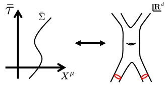
Figure 1: A path and a Riemann surface. The line on the left is a trajectory in the path integral. The trajectory parametrized by $\bar{\tau}$ from $\bar{\tau}=-\infty$ to $\bar{\tau}=\infty$, represents a Riemann surface with fixed punctures in $\mathbb{R}^{d}$ on the right.

The diffeomorphism times Weyl invariance of the action in (3.36) implies that the correlation function is given by

$$\Delta_{F}(X_{f};X_{i}|h_{f};h_{i})=Z\int_{h_{i},X_{i}}^{h_{f},X_{f}}\mathcal{D}h\mathcal{D}Xe^{-\lambda\chi}e^{-S_{s}},$$ (3.37)

where

$$S_{s}=\int_{-\infty}^{\infty}d\tau\int d\sigma\sqrt{h(\sigma,\tau)}\left(\frac{1}{2}h^{mn}(\sigma,\tau)\partial_{m}X^{\mu}(\sigma,\tau)\partial_{n}X_{\mu}(\sigma,\tau)\right),$$ (3.38)

and $\chi$ is the Euler number of the two-dimensional Riemannian manifold. For regularization, we divide the correlation function by $Z$ and the volume of the diffeomorphism and the Weyl transformation $V_{diff\times Weyl}$, by renormalizing $\tilde{H}^{\bot}_{d(\mu\bar{\sigma})}$. (3.37) is the all-order perturbative partition function of the string theory itself that possesses the moduli in the string theory. Especially, in string geometry, the consistency of the perturbation theory around the background (3.1) determines $d=26$ (the critical dimension).

4 Conclusion and Discussion

The Newtonian limit of any string geometry model around the flat background reproduces the perturbative string theory on the flat spacetime.

In case of coupling with a $u(1)$ gauge field, the perturbative vacuum solution in [1] and the Newtonian potential background in this paper coincide in the limit to reproduce the perturbative string. In this case, there exists accidentally an analytic solution that reduces to the Newtonian potential background in the limit, namely the perturbative vacuum solution. Thus, there does not exist two vacua to reproduce the perturbative string on the flat spacetime.

In general, it is natural to expect that one can reproduce the perturbative string theory on any supergravity background if one takes the Newtonian limit of any string geometry model around the corresponding background that includes the supergravity background [6].

Appendix A The relation between the perturbative vacuum background and the Newtonian potential background

The perturbative string theory is reproduced from fluctuations around a perturbative vacuum background of the Einstein-Hilbert action in string geometry theory coupled with a $u(1)$ gauge field in [1]. On the other hand, the perturbative string theory is also reproduced from fluctuations around the Newtonian potential background of an arbitrary gravitational action in string geometry theory in this paper. In this appendix, we clarify the relation between the perturbative vacuum background and the Newtonian potential background.

The background that represents the perturbative vacuum is given by

$$\bar{ds}^{2} = 2\lambda\bar{\rho}(\bar{h})N^{2}(X(\bar{\tau}))(dX^{d})^{2}+\int d\bar{\sigma}\bar{e}\int d\bar{\sigma}^{\prime}\bar{e}^{\prime}N^{\frac{2}{2-D}}(X(\bar{\tau}))\frac{\bar{e}^{3}(\bar{\sigma},\bar{\tau})}{\sqrt{\bar{h}(\bar{\sigma},\bar{\tau})}}\delta_{(\mu\bar{\sigma})(\mu^{\prime}\bar{\sigma}^{\prime})}dX^{(\mu\bar{\sigma})}dX^{(\mu^{\prime}\bar{\sigma}^{\prime})},$$

$$\bar{A}_{d} = i\sqrt{\frac{2-2D}{2-D}}\frac{\sqrt{2\lambda\bar{\rho}(\bar{h})}}{\sqrt{G_{N}}}N(X(\bar{\tau})),\qquad\bar{A}_{(\mu\bar{\sigma})}=0,$$ (A.1)

where $N(X(\bar{\tau}))=\frac{1}{1-\frac{1}{2}\alpha\phi(X(\bar{\tau}))}$. This is a solution to the equations of motion,

$$R_{IJ}=G_{N}(\frac{1}{2}F_{IK}F_{J}^{K}+\frac{1}{2(2-D)}G_{IJ}|F|^{2}),$$ (A.2)

$$\nabla_{K}F^{KI}=0.$$ (A.3)

By expanding this background metric up to the first order in $\alpha$, we obtain the Newtonian potential background (3.1). The contribution from the solution to the right-hand side of (A.2) becomes 0 in the first order because the contribution from the gauge field starts from the second order. Then, the solution satisfies (3.2). In section 3, we find that the part of the action in the second order in the fluctuations (3.16) coincides with the one obtained in [1] by rescaling an overall factor of the potential (3.4), which is a solution of (3.3), although there are contributions from the fluctuations around the background of the $u(1)$ gauge field.

Therefore, the perturbative string theory is reproduced in the case of the string geometry model coupled with the $u(1)$ gauge field by the same mechanism both in [1] and in this paper. Thus, the Newtonian limit is a natural generalization of reproducing the perturbative string theory in [1] to the case of any string geometry model.

Appendix B Explicit form of the Lagrangian up to the second order in the fluctuations.

Here we provide the explicit form of (3.9):

where we use short notation: we use indices $i$ instead of $(\mu\bar{\sigma})$ and all the indices are summed up. For an example,

$$\bar{\alpha}^{-1}_{i}\partial_{i}\phi\partial^{i}\tilde{H}_{dd}={\rm i}\int d\bar{\sigma}\bar{e}\times\frac{\sqrt{\bar{h}}}{\bar{e}^{3}}\times\left(\sum_{\mu=0}^{d-1}\partial_{\bar{\sigma}}X_{\mu}(\bar{\tau})\partial_{X^{\mu}(\bar{\tau})}\tilde{H}_{dd}\right).$$ (B.2)

References

[1]
M. Sato,
“String geometry and nonperturbative formulation of string theory,”
Int. J. Mod. Phys. A 34, no. 23, 1950126 (2019)
arXiv:1709.03506 [hep-th].
[2]
M. Sato and Y. Sugimoto,
Nucl. Phys. B 956 115019 (2020)
[arXiv:1903.05775 [hep-th]].
[3]I. M. Krichever, S. P. Novikov, “Algebras of Virasoro type, Riemann surfaces and the structure of soliton theory,” Funct. Anal. Appl. 21 (1987) 126
[4]I. M. Krichever, S. P. Novikov, “Virasoro-type algebras, Riemann surfaces and strings in Minkowsky space,” Funct. Anal. Appl. 21 (1987) 294
[5]E.S. Fradkin, D.M. Gitman, “Path integral representation for the relativistic particle propagators and BFV quantization,” Phys. Rev. D44 (1991) 3230
[6]
M. Honda and M. Sato,
Int. J. Mod. Phys. A 35, no.27, 2050176 (2020)
[arXiv:2003.12487 [hep-th]].