Online Passive-Aggressive Total-Error-Rate Minimization

Abstract

We provide a new online learning algorithm which utilizes online passive-aggressive learning (PA) and total-error-rate minimization (TER) for binary classification. The PA learning establishes not only large margin training but also the capacity to handle non-separable data. The TER learning on the other hand minimizes an approximated classification error based objective function. We propose an online PATER algorithm which combines those useful properties. In addition, we also present a weighted PATER algorithm to improve the ability to cope with data imbalance problems. Experimental results demonstrate that the proposed PATER algorithms achieves better performances in terms of efficiency and effectiveness than the existing state-of-the-art online learning algorithms in real-world data sets.

1 Introduction

Online learning has been widely studied and efficiently applied to sequentially arriving data problems that cannot be solved by batch learning (Cesa-Bianchi & Lugosi, 2006; Shalev-Shwartz, 2011; Hoi et al., 2018). In online binary classification, Perceptron (Rosenblatt, 1958) is one of the most popular algorithms based on the first-order information. The Perceptron adopts the following step loss function to minimize misclassification:

$$\ell_{step}(\boldsymbol{w})=\left\{\begin{array}[]{ c c }0&\mathbf{\boldsymbol{w}\cdot x}_{t}\geq 0\\ 1&\mathbf{\boldsymbol{w}\cdot x}_{t}<0\end{array}\right.,$$ (1)

where $\boldsymbol{w}\in\mathbb{R}^{d}$ is a parameter vector, and $\mathbf{x}_{t}\in\mathbb{R}^{d}$ is a sample vector at time $t$. In view of margin based learning, online passive-aggressive learning (PA) (Crammer et al., 2006) has been successfully developed as a notable online learning method. The PA updates their learning parameters with a large margin obtained by the following hinge loss function:

$$\ell_{hinge}(\boldsymbol{w})=\left\{\begin{array}[]{ c c }0&y_{t}\left(\mathbf{\boldsymbol{w}\cdot x}_{t}\right)\geq 1\\ 1-y_{t}\left(\mathbf{\boldsymbol{w}\cdot x}_{t}\right)&y_{t}\left(\mathbf{\boldsymbol{w}\cdot x}_{t}\right)<1\end{array}\right.,$$ (2)

where $\displaystyle y_{t}\in\{-1,1\}$ is a target label. The PA also accommodates non-separable data problems by not assuming data separability. In the use of the second-order information, the second-order perceptron (Cesa-Bianchi et al., 2005), the confidence weighted learning (Dredze et al., 2008), the adaptive regularization of weights learning (Crammer et al., 2009) have received considerable attention. Although the second-order information ensures the faster optimization convergence, the use of the first-order information is still reasonably attractive due to its simplicity.

Different from the margin based learning, Total-Error-Rate minimization (TER) based learning (Toh, 2008) has been introduced with a classification error approximation for binary classification (see Section 2.2). The TER takes two different step loss functions for false negative and false positive involved in the confusion matrix of binary classification. In order to achieve a deterministic global solution and avoid local solutions, the TER objective function adopts a quadratic approximation to the step function for the desired convexity. However, the above TER based solution has constructed a batch learning solution that has poor scalability for large-scale and real-time applications.

In this paper, we introduce a new online learning algorithm which can put in use the properties of PA and TER and overcome their individual shortcomings by combining them in which we call PATER for online binary classification. In addition, motivated by a weighted accuracy scheme (Brodersen et al., 2010), we also propose a weighted PATER (wPATER) method for data imbalance problems. Our empirical results demonstrate that the proposed methods show promising performances on 31 real-world data sets in terms of efficiency and effectiveness.

2 Preliminaries

2.1 Online Passive-Aggressive Learning (PA)

We introduce online Passive-Aggressive learning (PA) which is one of the popular online learning methods of linear classifiers for binary classification (Crammer et al., 2006). The optimization problem of the PA is as follows:

$${{\boldsymbol{w}}_{t+1}}=\arg\min\frac{1}{2}{\left\|{{\boldsymbol{w}}-{{\boldsymbol{w}}_{t}}}\right\|^{2}}\text{~{}~{}~{}}s.t.\text{~{}~{}~{}}\ell_{hinge}(\boldsymbol{w})=0,$$ (3)

By solving this optimization problem, the PA solution is given by:

$${{\boldsymbol{w}}_{t+1}}={{\boldsymbol{w}}_{t}}+\tau_{t}y_{t}\mathbf{x}_{t},$$ (4)

where $\tau_{t}=\frac{\ell_{hinge}(\boldsymbol{w})}{\left\|\mathbf{x}_{t}\right\|^{2}}$ is a Lagrange multiplier under the Karush-Khun-Tucker (KKT) condition (Boyd & Vandenberghe, 2004). The online PA solution is passively updated when the loss is close zero, whereas it is aggressively updated when it suffered from a significant loss.

2.2 Total-Error-Rate (TER) Minimization

In (Toh, 2008), a Total-Error-Rate (TER) has been utilized in an optimization problem for binary classification. The TER is defined as the sum of the False Positive Rate (FPR) and the False Negative Rate (FNR):

$$\ell_{step}^{TER}(\boldsymbol{w}) =FPR+FNR$$ (5)

$$=\frac{1}{n^{-}}\sum^{n^{-}}_{i=1}\ell_{step}^{FP}(\boldsymbol{w})+\frac{1}{n^{+}}\sum^{n^{+}}_{j=1}\ell_{step}^{FN}(\boldsymbol{w}),$$

where

$$\begin{array}[]{c}\ell_{step}^{FP}(\boldsymbol{w})=\left\{\begin{array}[]{ c c }0&-\mathbf{\boldsymbol{w}\cdot x}^{-}_{t}\geq 0\\ 1&-\mathbf{\boldsymbol{w}\cdot x}^{-}_{t}<0\end{array}\right.,\\ \\ \ell_{step}^{FN}(\boldsymbol{w})=\left\{\begin{array}[]{ c c }0&\phantom{-}\mathbf{\boldsymbol{w}\cdot x}^{+}_{t}\geq 0\\ 1&\phantom{-}\mathbf{\boldsymbol{w}\cdot x}^{+}_{t}<0\end{array}\right..\end{array}$$ (6)

$n^{-}$ and $n^{+}$ is the numbers of negative and positive samples respectively $(n=n^{-}+n^{+})$. The two superscripts, $-$ and $+$, are for indication of each class. The TER objective function has been presented based on the quadratic approximation to the two step loss functions of FP and FN as follows:

$${{\boldsymbol{w}}} =\arg\min\frac{1}{n^{-}}\sum^{n^{-}}_{i=1}\ell_{quad}^{FP}(\boldsymbol{w})+\frac{1}{n^{+}}\sum^{n^{+}}_{j=1}\ell_{quad}^{FN}(\boldsymbol{w}),$$ (7)

$$=\arg\min\frac{1}{{2n^{-}}}\sum\limits_{i=1}^{n^{-}}{{{\left({y_{i}^{-}-({\boldsymbol{w}}\cdot{\bf{x}}_{i}^{-})}\right)}^{2}}}+\frac{1}{{2n^{+}}}\sum\limits_{j=1}^{n^{+}}{{{\left({y_{j}^{+}-({\boldsymbol{w}}\cdot{\bf{x}}_{j}^{+})}\right)}^{2}}},$$

where

$$\begin{array}[]{c}\ell_{quad}^{FP}(\boldsymbol{w})={{{\left({y^{-}-({\boldsymbol{w}}\cdot{\bf{x}}^{-})}\right)}^{2}}},\\ \\ \ell_{quad}^{FN}(\boldsymbol{w})={{{\left({y^{+}-({\boldsymbol{w}}\cdot{\bf{x}}^{+})}\right)}^{2}}},\end{array}$$ (8)

which yields a closed-form solution related to weighted least-squares as

$$\boldsymbol{w}=(\mathbf{X}^{T}\mathbf{WX})^{-1}\mathbf{X}^{T}\mathbf{Wy},$$ (9)

where $\mathbf{X}=\left[\mathbf{X}^{-},\mathbf{X}^{+}\right]^{T}$ includes two sample matrices for negative and positive classes. $\mathbf{W}=diag\begin{pmatrix}\begin{bmatrix}\frac{1}{n^{-}}\,,\,\dotsc\,,\,\frac{1}{n^{-}}\,,\,\frac{1}{n^{+}}\,,\,\dotsc\,,\,\frac{1}{n^{+}}\end{bmatrix}\end{pmatrix}$ is a weight matrix that includes two different weights for the negative and positive classes. $\mathbf{y}=\begin{bmatrix}-1,\,\dotsc,\,-1,\,1,\,\dotsc,\,1\end{bmatrix}$ is the target vector. The batch mode TER solution handles binary classification problems by approximately counting the misclassified samples using the two different weights, $1\over n^{-}$ and $1\over n^{+}$.

3 Online Passive-Aggressive Total-Error-Rate Minimization (PATER)

In this section, based on the online PA learning, we present an online TER minimization algorithm (PATER). We start by addressing the two step loss functions $\ell_{step}^{FP}(\boldsymbol{w})$ and $\ell_{step}^{FN}(\boldsymbol{w})$ of TER. Similar to the hinge loss function in (2), these $\ell_{step}^{FP}(\boldsymbol{w})$ and $\ell_{step}^{FN}(\boldsymbol{w})$ can be rewritten as:

$$\begin{array}[]{c}\ell_{hinge}^{FP}(\boldsymbol{w})=\left\{\begin{array}[]{ c c }0&-\mathbf{\boldsymbol{w}\cdot x}^{-}_{t}\geq 1\\ 1+\mathbf{\boldsymbol{w}\cdot x}^{-}_{t}&-\mathbf{\boldsymbol{w}\cdot x}^{-}_{t}<1\end{array}\right.,\\ \\ \ell_{hinge}^{FN}(\boldsymbol{w})=\left\{\begin{array}[]{ c c }0&\phantom{-}\mathbf{\boldsymbol{w}\cdot x}^{+}_{t}\geq 1\\ 1-\mathbf{\boldsymbol{w}\cdot x}^{+}_{t}&\phantom{-}\mathbf{\boldsymbol{w}\cdot x}^{+}_{t}<1\end{array}\right..\end{array}$$ (10)

Based on $\ell_{hinge}^{FP}(\boldsymbol{w})$ and $\ell_{hinge}^{FN}(\boldsymbol{w})$ in (10), a new TER loss function is given by:

$$\ell_{hinge}^{TER}(\boldsymbol{w})=\frac{1}{n^{-}}\sum^{n^{-}}_{i=1}\ell_{hinge}^{FP}(\boldsymbol{w})+\frac{1}{n^{+}}\sum^{n^{+}}_{j=1}\ell_{hinge}^{FN}(\boldsymbol{w})$$ (11)

Similar to the PA objective function in (3), a new TER objective function using (11) can be written as:

$${{\boldsymbol{w}}_{t+1}}=\arg\min\frac{1}{2}{\left\|{{\boldsymbol{w}}-{{\boldsymbol{w}}_{t}}}\right\|^{2}}\text{~{}~{}~{}}s.t.\text{~{}~{}~{}}\ell_{hinge}^{TER}(\boldsymbol{w})=0.$$ (12)

The Lagrangian of optimization problem for TER minimization can then be defined as follows:

$$\mathscr{L}(\boldsymbol{w},\tau) =\frac{1}{2}\|\boldsymbol{w}-\boldsymbol{w}_{t}\|^{2}$$ (13)

$$\phantom{=}+\tau_{t}\left(\frac{1}{n^{-}_{t}}\sum^{n^{-}_{t}}_{i=1}1+\mathbf{\boldsymbol{w}\cdot x}^{-}_{i}+\frac{1}{n^{+}_{t}}\sum^{n^{+}_{t}}_{j=1}1-\mathbf{\boldsymbol{w}\cdot x}^{+}_{j}\right).$$

Taking the derivative of $\mathscr{L}(\boldsymbol{w},\tau)$ with respect to $\boldsymbol{w}$ and setting it to zero as:

$$\nabla_{\boldsymbol{w}}\mathscr{L}(\boldsymbol{w},\tau)=\boldsymbol{w}-\boldsymbol{w}_{t}+\tau_{t}\left(\frac{1}{n^{-}_{t}}\sum^{n^{-}_{t}}_{i=1}\mathbf{x}^{-}_{i}-\frac{1}{n^{+}_{t}}\sum^{n^{+}_{t}}_{j=1}\mathbf{x}^{+}_{j}\right)=0,$$ (14)

the PATER solution $\boldsymbol{w}$ is given by:

$$\boldsymbol{w}=\boldsymbol{w}_{t}-\tau_{t}\left(\frac{1}{n^{-}_{t}}\sum^{n^{-}_{t}}_{i=1}\mathbf{x}^{-}_{i}-\frac{1}{n^{+}_{t}}\sum^{n^{+}_{t}}_{j=1}\mathbf{x}^{+}_{j}\right).$$ (15)

In order to transform the two summation terms into vectorized recursive forms in (15), the PATER solution $\boldsymbol{w}$ can be rewritten as:

$$\boldsymbol{w} =\boldsymbol{w}_{t}-\tau_{t}\left(\left(\frac{n^{-}_{t-1}}{n^{-}_{t}}\sum^{n^{-}_{t-1}}_{i=1}\frac{1}{n^{-}_{t-1}}\mathbf{x}^{-}_{i}+\lambda^{-}_{t}\frac{1}{n^{-}_{t}}\mathbf{x}_{t}\right)\right.$$ (16)

$$\phantom{=}\left.-\left(\frac{n^{+}_{t-1}}{n^{+}_{t}}\sum^{n^{+}_{t-1}}_{j=1}\frac{1}{n^{+}_{t-1}}\mathbf{x}^{+}_{j}+\lambda^{+}_{t}\frac{1}{n^{+}_{t}}\mathbf{x}_{t}\right)\right)$$

$$=\boldsymbol{w}_{t}-\tau_{t}\left(\left(\frac{n^{-}_{t-1}}{n^{-}_{t}}\mathbf{z}^{-}_{t-1}+\frac{\lambda^{-}_{t}}{n^{-}_{t}}\mathbf{x}_{t}\right)-\left(\frac{n^{+}_{t-1}}{n^{+}_{t}}\mathbf{z}^{+}_{t-1}+\frac{\lambda^{+}_{t}}{n^{+}_{t}}\mathbf{x}_{t}\right)\right)$$

$$=\boldsymbol{w}_{t}-\tau_{t}\left(\mathbf{z}^{-}_{t}-\mathbf{z}^{+}_{t}\right)$$

$$=\boldsymbol{w}_{t}+\tau_{t}\mathbf{z}_{t},$$

where $\lambda^{-}_{t}=\frac{1-y_{t}}{2}$ and $\lambda^{+}_{t}=\frac{1+y_{t}}{2}$ are indicators to select one class between the two classes at time $t$. $\mathbf{z}_{t}=\mathbf{z}^{+}_{t}-\mathbf{z}^{-}_{t}$, $\mathbf{z}^{-}_{t}=\frac{n^{-}_{t-1}}{n^{-}_{t}}\mathbf{z}^{-}_{t-1}+\frac{\lambda^{-}_{t}}{n^{-}_{t}}\mathbf{x}_{t}$, and $\mathbf{z}^{+}_{t}=\frac{n^{+}_{t-1}}{n^{+}_{t}}\mathbf{z}^{+}_{t-1}+\frac{\lambda^{+}_{t}}{n^{+}_{t}}\mathbf{x}_{t}$.

Substituting the parameter vector $\boldsymbol{w}$ with (16) in (13), we get

$$\mathscr{L}(\tau) =-\frac{1}{2}\tau^{2}\left\|\mathbf{z}_{t}\right\|^{2}$$ (17)

$$\phantom{=}+\tau\left(\frac{1}{n^{-}_{t}}\sum^{n^{-}_{t}}_{i=1}1+\boldsymbol{w}_{t}\mathbf{\cdot x}^{-}_{i}+\frac{1}{n^{+}_{t}}\sum^{n^{+}_{t}}_{j=1}1-\boldsymbol{w}_{t}\mathbf{\cdot x}^{+}_{j}\right).$$

In (17), the linearly increasing computational complexity $\mathscr{O}(dn_{t})$ of the summation terms is observed and caused by the dot product of $\boldsymbol{w}_{t}\mathbf{\cdot x}$ for each sample. To avoid this computation, two different versions, namely PATER-I and PATER-II, of (17) are given by:

$$\text{PATER-I: }\mathscr{L}(\tau) =-\frac{1}{2}\tau^{2}\left\|\mathbf{z}_{t}\right\|^{2}+\tau\left(\frac{\lambda^{-}_{t}}{n^{-}_{t}}\left(1+\boldsymbol{w}_{t}\mathbf{\cdot x}_{t}\right)\right.$$ (18)

$$\phantom{=}\left.+\frac{\lambda^{+}_{t}}{n^{+}_{t}}\left(1-\boldsymbol{w}_{t}\mathbf{\cdot x}_{t}\right)\right),$$

$$\text{PATER-II: }\mathscr{L}(\tau) =-\frac{1}{2}\tau^{2}\left\|\mathbf{z}_{t}\right\|^{2}+\tau\left(\frac{n^{-}_{t-1}}{n^{-}_{t}}k^{-}_{t-1}+\frac{\lambda^{-}_{t}}{n^{-}_{t}}\left(1+\boldsymbol{w}_{t}\mathbf{\cdot x}_{t}\right)\right.$$ (19)

$$\phantom{=}\left.+\frac{n^{+}_{t-1}}{n^{+}_{t}}k^{+}_{t-1}+\frac{\lambda^{+}_{t}}{n^{+}_{t}}\left(1-\boldsymbol{w}_{t}\mathbf{\cdot x}_{t}\right)\right)$$

$$=-\frac{1}{2}\tau^{2}\left\|\mathbf{z}_{t}\right\|^{2}+\tau\left(k^{-}_{t}+k^{+}_{t}\right),$$

where $k^{-}_{0}=k^{+}_{0}=0$, $k^{-}_{t}=\frac{n^{-}_{t-1}}{n^{-}_{t}}k^{-}_{t-1}+\frac{\lambda^{-}_{t}}{n^{-}_{t}}\left(1+\boldsymbol{w}_{t}\mathbf{\cdot x}_{t}\right)$, and $k^{+}_{t}=\frac{n^{+}_{t-1}}{n^{+}_{t}}k^{+}_{t-1}+\frac{\lambda^{+}_{t}}{n^{+}_{t}}\left(1-\boldsymbol{w}_{t}\mathbf{\cdot x}_{t}\right)$.

Taking the derivative of $\mathscr{L}(\tau)$ in (18) and (19) with respect to $\tau$ and setting it zero as:

$$\text{PATER-I: }\frac{\partial\mathscr{L}(\tau)}{\partial\tau} =-\tau\left\|\mathbf{z}_{t}\right\|^{2}+\frac{\lambda^{-}_{t}}{n^{-}_{t}}\left(1+\boldsymbol{w}_{t}\mathbf{\cdot x}_{t}\right)$$ (20)

$$\phantom{=}+\frac{\lambda^{+}_{t}}{n^{+}_{t}}\left(1-\boldsymbol{w}_{t}\mathbf{\cdot x}_{t}\right)=0,$$

$$\text{PATER-II: }\frac{\partial\mathscr{L}(\tau)}{\partial\tau}=-\tau\left\|\mathbf{z}_{t}\right\|^{2}+k^{-}_{t}+k^{+}_{t}=0,$$ (21)

we get:

$$\text{PATER-I: }\tau_{t}=\frac{\frac{\lambda^{-}_{t}}{n^{-}_{t}}\left(1+\boldsymbol{w}_{t}\mathbf{\cdot x}_{t}\right)+\frac{\lambda^{+}_{t}}{n^{+}_{t}}\left(1-\boldsymbol{w}_{t}\mathbf{\cdot x}_{t}\right)}{\left\|\mathbf{z}_{t}\right\|^{2}},$$ (22)

$$\text{PATER-II: }\tau_{t}=\frac{k^{-}_{t}+k^{+}_{t}}{\left\|\mathbf{z}_{t}\right\|^{2}}.$$ (23)

Algorithm 1 Passive-Aggressive TER Minimization

  Input: a sample $\mathbf{x}_{t}\in\mathbb{R}^{d}$,           a label $y_{t}\in\{-1,+1\}$

  Initialize: $\boldsymbol{w}_{0}=\mathbf{z}_{0}^{-}=\mathbf{z}_{0}^{+}=\mathbf{0}$,               $n_{0}^{-}=n_{0}^{+}=k_{t}^{-}=k_{t}^{+}=0$

  for $t=1,\dots$  do

     Set $\lambda^{-}_{t}=\frac{1-y_{t}}{2}$ and $\lambda^{+}_{t}=\frac{1+y_{t}}{2}$

     Update $n_{t}^{-}=n_{t-1}^{-}+\lambda^{-}_{t}$,           $n_{t}^{+}=n_{t-1}^{+}+\lambda^{+}_{t}$

     Update $\mathbf{z}^{-}_{t}=\frac{n^{-}_{t-1}}{n^{-}_{t}}\mathbf{z}^{-}_{t-1}+\frac{\lambda^{-}_{t}}{n^{-}_{t}}\mathbf{x}_{t}$,           $\mathbf{z}^{+}_{t}=\frac{n^{+}_{t-1}}{n^{+}_{t}}\mathbf{z}^{+}_{t-1}+\frac{\lambda^{+}_{t}}{n^{+}_{t}}\mathbf{x}_{t}$

     Update $k^{-}_{t}=\frac{n^{-}_{t-1}}{n^{-}_{t}}k^{-}_{t-1}+\frac{\lambda^{-}_{t}}{n^{-}_{t}}\left(1+\boldsymbol{w}_{t-1}\mathbf{\cdot x}_{t}\right)$,           $k^{+}_{t}=\frac{n^{+}_{t-1}}{n^{+}_{t}}k^{+}_{t-1}+\frac{\lambda^{+}_{t}}{n^{+}_{t}}\left(1-\boldsymbol{w}_{t-1}\mathbf{\cdot x}_{t}\right)$

     Set $\mathbf{z}_{t}=\mathbf{z}^{+}_{t}-\mathbf{z}^{-}_{t}$

     Set $\tau_{t}$ as:        PATER-I: $\tau_{t}=\frac{\frac{\lambda^{-}_{t}}{n^{-}_{t}}\left(1+\boldsymbol{w}_{t-1}\mathbf{\cdot x}_{t}\right)+\frac{\lambda^{+}_{t}}{n^{+}_{t}}\left(1-\boldsymbol{w}_{t-1}\mathbf{\cdot x}_{t}\right)}{\left\|\mathbf{z}_{t}\right\|^{2}}$        PATER-II: $\tau_{t}=\frac{k^{-}_{t}+k^{+}_{t}}{\left\|\mathbf{z}_{t}\right\|^{2}}$

     Update $\boldsymbol{w}_{t}=\boldsymbol{w}_{t-1}+\tau_{t}\mathbf{z}_{t}$

  end for

3.1 Summary

The pseudo code of the proposed PATER algorithm is given in Algorithm 1. The main difference from the PA learning is that the PATER solution is given by the newly derived objective function (12) utilizing the PA and the TER learning together. The main difference between PATER-I and PATER-II is that PATER-I includes an instantaneous loss while PATER-II uses an approximately accumulated loss in $\tau_{t}$.

4 Weighted PATER Minimization (wPATER)

In this section, we present a weighted PATER algorithm (wPATER) inspired by the concept of a balanced accuracy for performance evaluation in (Brodersen et al., 2010). In order to address imbalanced data sets, a balanced accuracy is defined as $\displaystyle bAcc=\frac{1}{2}\left(\frac{TN}{n^{-}}+\frac{TP}{n^{+}}\right)$, where TN is the True Negative, and TP is the True Positive. In view of a generalized design, a weighted accuracy can be written as:

$$wAcc=\alpha^{-}\frac{TN}{n^{-}}+\alpha^{+}\frac{TP}{n^{+}},$$ (24)

where $bAcc$ is given by $\alpha^{-}=\alpha^{+}=0.5$. In a similar manner to this weighted accuracy, a weighted TER (wTER) can be defined as

$$wTER=\alpha^{-}\frac{FP}{n^{-}}+\alpha^{+}\frac{FN}{n^{+}}.$$ (25)

Based on the wTER definition, similar to (11), a new wTER loss function is given by:

$$\ell_{hinge}^{wTER}(\boldsymbol{w})=\frac{\alpha^{-}}{n^{-}}\sum^{n^{-}}_{i=1}\ell_{hinge}^{FP}(\boldsymbol{w})+\frac{\alpha^{+}}{n^{+}}\sum^{n^{+}}_{j=1}\ell_{hinge}^{FN}(\boldsymbol{w}).$$ (26)

Accordingly, the wTER objective function can be written as:

$${{\boldsymbol{w}}_{t+1}}=\arg\min\frac{1}{2}{\left\|{{\boldsymbol{w}}-{{\boldsymbol{w}}_{t}}}\right\|^{2}}\text{~{}~{}~{}}s.t.\text{~{}~{}~{}}\ell_{hinge}^{wTER}(\boldsymbol{w})=0.$$ (27)

Similar to (13), the Lagrangian of the optimization problem can then be defined as:

$$\mathscr{L}(\boldsymbol{w},\tau) =\frac{1}{2}\|\boldsymbol{w}-\boldsymbol{w}_{t}\|^{2}$$ (28)

$$\phantom{=}+\tau_{t}\left(\frac{\alpha^{-}}{n^{-}_{t}}\sum^{n^{-}_{t}}_{i=1}1+\mathbf{\boldsymbol{w}\cdot x}^{-}_{i}+\frac{\alpha^{+}}{n^{+}_{t}}\sum^{n^{+}_{t}}_{j=1}1-\mathbf{\boldsymbol{w}\cdot x}^{+}_{j}\right).$$

Similarly, the wPATER solution $\boldsymbol{w}$ is given by:

$$\boldsymbol{w}=\boldsymbol{w}_{t}+\tau_{t}\mathbf{z}_{t},$$ (29)

where $\mathbf{z}_{t}=\alpha^{+}\mathbf{z}^{+}_{t}-\alpha^{-}\mathbf{z}^{-}_{t}$. Next, similar to (17), we get:

$$\mathscr{L}(\tau) =-\frac{1}{2}\tau^{2}\left\|\mathbf{z}_{t}\right\|^{2}$$ (30)

$$\phantom{=}+\tau\left(\frac{\alpha^{-}}{n^{-}_{t}}\sum^{n^{-}_{t}}_{i=1}1+\boldsymbol{w}_{t}\mathbf{\cdot x}^{-}_{i}+\frac{\alpha^{+}}{n^{+}_{t}}\sum^{n^{+}_{t}}_{j=1}1-\boldsymbol{w}_{t}\mathbf{\cdot x}^{+}_{j}\right).$$

Algorithm 2 Weighted PATER Minimization

  Input: a sample $\mathbf{x}_{t}\in\mathbb{R}^{d}$,           a label $y_{t}\in\{-1,+1\}$

  Initialize: $\boldsymbol{w}_{0}=\mathbf{z}_{0}^{-}=\mathbf{z}_{0}^{+}=\mathbf{0}$,               $n_{0}^{-}=n_{0}^{+}=k_{t}^{-}=k_{t}^{+}=0$,               $\alpha^{-}>0,\alpha^{+}>0$

  for $t=1,\dots$  do

     Set $\lambda^{-}_{t}=\frac{1-y_{t}}{2}$ and $\lambda^{+}_{t}=\frac{1+y_{t}}{2}$

     Update $n_{t}^{-}=n_{t-1}^{-}+\lambda^{-}_{t}$,           $n_{t}^{+}=n_{t-1}^{+}+\lambda^{+}_{t}$

     Update $\mathbf{z}^{-}_{t}=\frac{n^{-}_{t-1}}{n^{-}_{t}}\mathbf{z}^{-}_{t-1}+\frac{\lambda^{-}_{t}}{n^{-}_{t}}\mathbf{x}_{t}$,           $\mathbf{z}^{+}_{t}=\frac{n^{+}_{t-1}}{n^{+}_{t}}\mathbf{z}^{+}_{t-1}+\frac{\lambda^{+}_{t}}{n^{+}_{t}}\mathbf{x}_{t}$

     Update $k^{-}_{t}=\frac{n^{-}_{t-1}}{n^{-}_{t}}k^{-}_{t-1}+\frac{\lambda^{-}_{t}}{n^{-}_{t}}\left(1+\boldsymbol{w}_{t-1}\mathbf{\cdot x}_{t}\right)$,           $k^{+}_{t}=\frac{n^{+}_{t-1}}{n^{+}_{t}}k^{+}_{t-1}+\frac{\lambda^{+}_{t}}{n^{+}_{t}}\left(1-\boldsymbol{w}_{t-1}\mathbf{\cdot x}_{t}\right)$

     Set $\mathbf{z}_{t}=\alpha^{+}\mathbf{z}^{+}_{t}-\alpha^{-}\mathbf{z}^{-}_{t}$

     Set $\tau_{t}$ as:        wPATER-I: $\tau_{t}=\frac{\frac{\alpha^{-}\lambda^{-}_{t}}{n^{-}_{t}}\left(1+\boldsymbol{w}_{t-1}\mathbf{\cdot x}_{t}\right)+\frac{\alpha^{+}\lambda^{+}_{t}}{n^{+}_{t}}\left(1-\boldsymbol{w}_{t-1}\mathbf{\cdot x}_{t}\right)}{\left\|\mathbf{z}_{t}\right\|^{2}}$        wPATER-II: $\tau_{t}=\frac{\alpha^{-}k^{-}_{t}+\alpha^{+}k^{+}_{t}}{\left\|\mathbf{z}_{t}\right\|^{2}}$

     Update $\boldsymbol{w}_{t}=\boldsymbol{w}_{t-1}+\tau_{t}\mathbf{z}_{t}$

  end for

Table 1: Summary of the 31 real-world data sets for binary classification.

	No.	Data sets	#cases(original)	#feat	Ratio	#miss	No.	Data sets	#cases(original)	#feat	Ratio	#miss
	1	Monks-3	122(423)	6	0.98	No	17	Blood-transfusion	748	4	0.31	No
	2	Monks-1	124(423)	6	1.01	No	18	Pima-diabetes	768	8	0.54	No
	3	Monks-2	169(423)	6	0.62	No	19	Mammographic	830(961)	5	0.95	131
	4	Wpbc	194(198)	33	0.31	4	20	Tic-tac-toe	958	9	0.53	No
	5	Parkinsons	195	22	3.15	No	21	Statlog-german	1,000	24	2.34	No
	6	Sonar	208	60	1.16	No	22	Ozone-eight	1,847(2,534)	72	0.07	687
	7	SPECTF-heart	267	44	3.89	No	23	Ozone-one	1,848(2,536)	72	0.03	688
	8	StatLog-heart	270	13	0.80	No	24	20News-talk	1,848	3	1.04	No
	9	BUPA-liver	345	6	1.39	No	25	20News-comp	1,937	3	0.98	No
	10	Ionosphere	351	34	0.56	No	26	20News-sci	1,971	3	1.01	No
	11	Votes	435	16	1.60	Yes	27	Spambase	4,601	57	0.65	No
	12	Musk-clean-1	476	166	0.77	No	28	Mushroom	5,644(8,124)	22	1.62	Attr#11
	13	Wdbc	569	30	1.69	No	29	Cod-rna	59,535	8	0.50	No
	14	Credit-app	653(690)	15	1.21	37	30	Ijcnn1	141,691	22	0.11	No
	15	Breast-cancer-W	683(699)	9	0.54	16	31	Skin-nonskin	245,057	3	0.26	No
	16	Statlog-australian	690	14	0.81	Yes

Table 2: Comparison of average accuracies with its standard deviations and ranks.

No.	Data sets	PE	PA	PATER-I	PATER-II	wPATER-I	wPATER-II
1	Monks-3	70.902 $\pm$ 6.446 (6)	71.066 $\pm$ 4.795 (5)	75.574 $\pm$ 4.218 (4)	75.738 $\pm$ 3.821 (3)	75.984 $\pm$ 4.297 (2)	77.295 $\pm$ 4.675 (1)
2	Monks-1	64.355 $\pm$ 6.407 (5)	64.355 $\pm$ 7.760 (6)	64.919 $\pm$ 7.454 (4)	67.177 $\pm$ 3.747 (2)	67.097 $\pm$ 5.976 (3)	69.919 $\pm$ 3.891 (1)
3	Monks-2	54.195 $\pm$ 6.741 (3)	52.426 $\pm$ 6.664 (4)	49.235 $\pm$ 4.245 (6)	50.049 $\pm$ 5.094 (5)	61.720 $\pm$ 4.682 (2)	62.132 $\pm$ 4.186 (1)
4	Wpbc	67.835 $\pm$ 5.274 (3)	65.670 $\pm$ 5.558 (4)	59.021 $\pm$ 3.899 (5)	55.309 $\pm$ 5.375 (6)	72.113 $\pm$ 4.443 (1)	69.278 $\pm$ 4.749 (2)
5	Parkinsons	76.563 $\pm$ 5.060 (3)	78.150 $\pm$ 6.388 (2)	67.586 $\pm$ 3.124 (5)	66.408 $\pm$ 2.809 (6)	82.618 $\pm$ 4.467 (1)	74.822 $\pm$ 5.296 (4)
6	Sonar	69.904 $\pm$ 5.202 (5)	72.067 $\pm$ 3.424 (4)	72.788 $\pm$ 4.335 (2)	69.615 $\pm$ 5.242 (6)	74.471 $\pm$ 3.618 (1)	72.115 $\pm$ 6.378 (3)
7	SPECTF-heart	72.361 $\pm$ 3.659 (3)	72.473 $\pm$ 4.124 (2)	55.580 $\pm$ 3.530 (5)	53.633 $\pm$ 2.681 (6)	76.405 $\pm$ 3.015 (1)	70.447 $\pm$ 3.898 (4)
8	Statlog-heart	78.667 $\pm$ 4.303 (5)	77.667 $\pm$ 5.370 (6)	81.000 $\pm$ 2.867 (4)	82.815 $\pm$ 2.704 (2)	82.111 $\pm$ 2.956 (3)	84.037 $\pm$ 2.046 (1)
9	BUPA-liver	58.233 $\pm$ 4.359 (4)	57.769 $\pm$ 3.575 (5)	59.535 $\pm$ 2.958 (2)	54.463 $\pm$ 3.414 (6)	61.161 $\pm$ 3.785 (1)	58.550 $\pm$ 4.726 (3)
10	Ionosphere	80.573 $\pm$ 4.352 (5)	84.302 $\pm$ 2.641 (2)	81.711 $\pm$ 5.333 (3)	73.478 $\pm$ 6.391 (6)	85.128 $\pm$ 3.707 (1)	81.367 $\pm$ 4.494 (4)
11	Votes	90.481 $\pm$ 3.674 (3)	91.605 $\pm$ 3.796 (2)	90.369 $\pm$ 1.994 (4)	87.999 $\pm$ 1.633 (6)	92.368 $\pm$ 1.608 (1)	88.644 $\pm$ 1.396 (5)
12	Musk-clearn-1	70.399 $\pm$ 5.390 (4)	70.546 $\pm$ 5.285 (3)	74.958 $\pm$ 3.450 (2)	62.836 $\pm$ 6.602 (6)	75.546 $\pm$ 3.032 (1)	63.592 $\pm$ 5.455 (5)
13	Wdbc	94.728 $\pm$ 2.591 (4)	95.518 $\pm$ 1.985 (3)	96.010 $\pm$ 0.963 (2)	93.145 $\pm$ 1.369 (6)	96.116 $\pm$ 0.886 (1)	93.479 $\pm$ 1.225 (5)
14	Credit-app	80.503 $\pm$ 5.775 (6)	81.682 $\pm$ 5.579 (5)	84.349 $\pm$ 1.957 (4)	85.284 $\pm$ 1.519 (2)	84.441 $\pm$ 1.818 (3)	85.376 $\pm$ 1.581 (1)
15	Breast-cancer-W	95.623 $\pm$ 2.029 (5)	95.491 $\pm$ 2.126 (6)	96.969 $\pm$ 0.858 (3)	96.881 $\pm$ 0.581 (4)	97.115 $\pm$ 0.792 (2)	97.438 $\pm$ 0.593 (1)
16	Statlog-australian	78.841 $\pm$ 5.582 (6)	79.493 $\pm$ 5.908 (5)	84.217 $\pm$ 2.009 (4)	85.507 $\pm$ 1.128 (2)	84.290 $\pm$ 1.702 (3)	85.580 $\pm$ 1.289 (1)
17	Blood-transfusion	68.436 $\pm$ 8.363 (3)	66.444 $\pm$ 11.36 (4)	59.024 $\pm$ 9.134 (6)	62.794 $\pm$ 3.059 (5)	76.377 $\pm$ 1.439 (2)	76.912 $\pm$ 1.255 (1)
18	Pima-diabetes	68.099 $\pm$ 3.994 (5)	69.505 $\pm$ 3.482 (4)	66.797 $\pm$ 5.272 (6)	72.057 $\pm$ 1.466 (2)	70.208 $\pm$ 3.635 (3)	74.740 $\pm$ 1.262 (1)
19	Mammographic	70.482 $\pm$ 16.87 (6)	72.241 $\pm$ 13.58 (5)	76.494 $\pm$ 8.903 (4)	81.349 $\pm$ 1.096 (2)	78.012 $\pm$ 6.420 (3)	81.602 $\pm$ 1.023 (1)
20	Tic-tac-toe	55.929 $\pm$ 5.301 (5)	56.013 $\pm$ 5.805 (4)	52.453 $\pm$ 4.740 (6)	56.983 $\pm$ 2.743 (3)	65.376 $\pm$ 1.731 (2)	67.056 $\pm$ 1.786 (1)
21	Statlog-german	68.470 $\pm$ 3.223 (4)	66.410 $\pm$ 4.967 (5)	63.120 $\pm$ 2.671 (6)	68.630 $\pm$ 1.454 (3)	71.910 $\pm$ 1.475 (2)	75.630 $\pm$ 1.260 (1)
22	Ozone-eight	89.924 $\pm$ 3.083 (3)	90.921 $\pm$ 3.164 (2)	52.528 $\pm$ 1.977 (6)	53.059 $\pm$ 1.154 (5)	92.534 $\pm$ 0.891 (1)	67.845 $\pm$ 5.597 (4)
23	Ozone-one	92.516 $\pm$ 5.130 (3)	95.070 $\pm$ 3.190 (2)	50.168 $\pm$ 1.519 (5)	49.800 $\pm$ 0.945 (6)	96.374 $\pm$ 0.478 (1)	79.015 $\pm$ 10.88 (4)
24	20News-talk	49.957 $\pm$ 1.196 (4)	49.854 $\pm$ 1.030 (5)	49.811 $\pm$ 1.829 (6)	50.060 $\pm$ 0.986 (3)	51.292 $\pm$ 2.147 (1)	50.838 $\pm$ 1.230 (2)
25	20News-comp	54.544 $\pm$ 4.127 (5)	53.376 $\pm$ 5.999 (6)	58.839 $\pm$ 6.779 (3)	57.495 $\pm$ 6.426 (4)	63.676 $\pm$ 6.350 (1)	59.172 $\pm$ 9.193 (2)
26	20News-sci	72.572 $\pm$ 10.24 (4)	69.980 $\pm$ 9.689 (5)	73.310 $\pm$ 9.626 (3)	65.591 $\pm$ 5.703 (6)	74.420 $\pm$ 10.16 (2)	74.425 $\pm$ 6.073 (1)
27	Spambase	87.142 $\pm$ 2.570 (5)	86.707 $\pm$ 2.714 (6)	89.961 $\pm$ 1.743 (2)	89.048 $\pm$ 0.462 (4)	90.915 $\pm$ 0.894 (1)	89.641 $\pm$ 0.411 (3)
28	Mushroom	91.357 $\pm$ 5.435 (4)	93.698 $\pm$ 3.097 (3)	93.820 $\pm$ 1.721 (2)	87.509 $\pm$ 0.593 (6)	94.341 $\pm$ 0.891 (1)	88.521 $\pm$ 0.761 (5)
29	Cod-rna	90.590 $\pm$ 1.627 (2)	90.669 $\pm$ 1.822 (1)	87.965 $\pm$ 1.843 (4)	69.606 $\pm$ 0.246 (6)	89.420 $\pm$ 2.441 (3)	77.571 $\pm$ 0.110 (5)
30	Ijcnn1	89.655 $\pm$ 1.811 (4)	90.342 $\pm$ 1.673 (3)	59.430 $\pm$ 3.303 (6)	65.847 $\pm$ 0.690 (5)	92.029 $\pm$ 0.266 (1)	90.426 $\pm$ 0.070 (2)
31	Skin-nonskin	88.917 $\pm$ 5.564 (3)	91.104 $\pm$ 4.185 (1)	89.302 $\pm$ 1.610 (2)	66.539 $\pm$ 4.338 (6)	88.209 $\pm$ 0.790 (4)	87.725 $\pm$ 0.077 (5)
	Average	75.573 $\pm$ 5.012 (4.19)	75.891 $\pm$ 4.863 (3.87)	71.511 $\pm$ 3.737 (4.06)	69.571 $\pm$ 2.757 (4.52)	79.477 $\pm$ 2.929 (1.77)	76.619 $\pm$ 3.125 (2.58)

In order to establish wPATER-I and wPATER-II, similar to (18) and (19), we get:

$$\text{wPATER-I: }\mathscr{L}(\tau) =-\frac{1}{2}\tau^{2}\left\|\mathbf{z}_{t}\right\|^{2}+\tau\left(\frac{\alpha^{-}\lambda^{-}_{t}}{n^{-}_{t}}\left(1+\boldsymbol{w}_{t}\mathbf{\cdot x}_{t}\right)\right.$$ (31)

$$\phantom{=}\left.+\frac{\alpha^{+}\lambda^{+}_{t}}{n^{+}_{t}}\left(1-\boldsymbol{w}_{t}\mathbf{\cdot x}_{t}\right)\right),$$

$$\text{wPATER-II: }\mathscr{L}(\tau) =-\frac{1}{2}\tau^{2}\left\|\mathbf{z}_{t}\right\|^{2}+\tau\left(\alpha^{-}k^{-}_{t}+\alpha^{+}k^{+}_{t}\right).$$ (32)

Taking the derivative of $\mathscr{L}(\tau)$ in (31) and (32) with respect to $\tau$ and setting it zero as:

$$\text{wPATER-I: }\frac{\partial\mathscr{L}(\tau)}{\partial\tau} =-\tau\left\|\mathbf{z}_{t}\right\|^{2}+\frac{\alpha^{-}\lambda^{-}_{t}}{n^{-}_{t}}\left(1+\boldsymbol{w}_{t}\mathbf{\cdot x}_{t}\right)$$ (33)

$$\phantom{=}+\frac{\alpha^{+}\lambda^{+}_{t}}{n^{+}_{t}}\left(1-\boldsymbol{w}_{t}\mathbf{\cdot x}_{t}\right)=0,$$

$$\text{wPATER-II: }\frac{\partial\mathscr{L}(\tau)}{\partial\tau}=-\tau\left\|\mathbf{z}_{t}\right\|^{2}+\alpha^{-}k^{-}_{t}+\alpha^{+}k^{+}_{t}=0,$$ (34)

we get:

$$\text{wPATER-I: }\tau_{t}=\frac{\frac{\alpha^{-}\lambda^{-}_{t}}{n^{-}_{t}}\left(1+\boldsymbol{w}_{t}\mathbf{\cdot x}_{t}\right)+\frac{\alpha^{+}\lambda^{+}_{t}}{n^{+}_{t}}\left(1-\boldsymbol{w}_{t}\mathbf{\cdot x}_{t}\right)}{\left\|\mathbf{z}_{t}\right\|^{2}},$$ (35)

$$\text{wPATER-II: }\tau_{t}=\frac{\alpha^{-}k^{-}_{t}+\alpha^{+}k^{+}_{t}}{\left\|\mathbf{z}_{t}\right\|^{2}}.$$ (36)

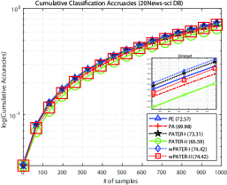
(a) 20News-sci

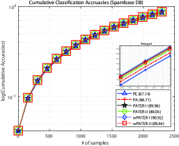
(b) Spambase

(c) Mushroom

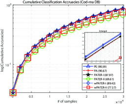
(d) Cod-rna

(e) Ijcnn1

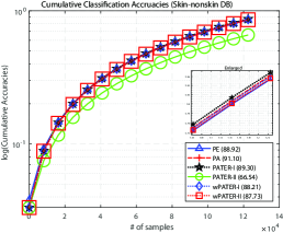
(f) Skin-nonskin

Figure 1: The cumulative classification accuracies along the online learning process. The enlarged figure is also drawn for detailed comparison. The brackets include the average accuracies.

4.1 Summary

The pseudo code of the proposed wPATER algorithm is given in Algorithm 2. The main difference from PATER is that wPATER has two weights, $\alpha^{-}$ and $\alpha^{+}$, as hyperparameters in its loss function (26) to address the imbalance data issue.

5 Experiments

In this section, we evaluate the performance of the proposed PATER and wPATER for binary classification. In terms of efficiency and effectiveness, the performance comparison is presented based on 31 real-world data sets.

5.1 Data sets and experimental settings

In our evaluation, 31 real-world data sets are obtained from UCI machine learning repository (Lichman, 2013), LIBSVM (Chang & Lin, 2011) and 20 Newsgroups which are popular in the NLP community. The description of the 31 data sets is summarized in Table 1. Each data set is conducted in a z-score normalization. The data set size ranges from 122 to 245,057 samples. The data imbalance ratio is calculated by $\frac{n^{+}}{n^{-}}$.

For comparison with competing state-of-the-arts, the following algorithms are used as baselines: the perceptron (PE) (Rosenblatt, 1958) and the online passive-aggressive algorithm (PA) (Crammer et al., 2006). The average accuracies and CPU times are recorded using 10 runs of 2-fold cross-validation for each algorithm.

In wPATER, the two weights are varied as $\alpha^{-},\alpha^{+}\in\{0.01,\ 0.1,\ 0.3,\ 0.5,\ 0.9,\ 0.99\}$. When one weight is changed, another weight is fixed at $1$ (i.e., $\alpha^{-}=0.1$, $\alpha^{+}=1$) to only address one side population of the imbalance binary classification problems.

Table 3: Evaluation of the best weights between $\alpha^{-}$ and $\alpha^{+}$ of the proposed wPATER for the data imbalance problems.

	Evaluation																															Sum
Data No.	1	2	3	4	5	6	7	8	9	10	11	12	13	14	15	16	17	18	19	20	21	22	23	24	25	26	27	28	29	30	31
Needed Weight (NW)	P	N	P	P	N	N	N	P	N	P	N	P	N	N	P	P	P	P	P	P	N	P	P	N	P	N	P	N	P	P	P
Best Weight (BW)	P	P	P	P	N	N	N	P	N	P	N	P	N	P	N	P	P	P	P	P	N	P	P	N	P	P	P	N	-	P	-
Results (BW equals NW)	1	0	1	1	1	1	1	1	1	1	1	1	1	0	0	1	1	1	1	1	1	1	1	1	1	0	1	1	0	1	0	25

Notes: ‘N’ and ‘P’ indicate the negative and posivie classes respectively. In NW, ‘N’ is given if $\frac{n^{+}}{n^{-}}\geq 1$; otherwise ‘P’ is given. $\frac{n^{+}}{n^{-}}$ is the data imbalance ratio shown in Table 1. In BW, ‘N’ is given if the best performance is obtained from the $\alpha^{-}$ variation; otherwise ‘P’ is given.

Table 4: Comparison of average CPU times in seconds.

No.	Data sets	PE	PA	PATER-I	PATER-II	wPATER-I	wPATER-II
1	Monks-3	0.0008	0.0013	0.0017	0.0019	0.0006	0.0009
2	Monks-1	0.0006	0.0006	0.0008	0.0009	0.0006	0.0008
3	Monks-2	0.0007	0.0008	0.0010	0.0012	0.0009	0.0012
4	Wpbc	0.0006	0.0008	0.0011	0.0014	0.0010	0.0014
5	Parkinsons	0.0006	0.0007	0.0010	0.0014	0.0009	0.0013
6	Sonar	0.0007	0.0009	0.0013	0.0016	0.0011	0.0015
7	SPECTF-heart	0.0008	0.0011	0.0015	0.0019	0.0014	0.0018
8	Statlog-heart	0.0008	0.0010	0.0014	0.0019	0.0012	0.0018
9	BUPA-liver	0.0011	0.0014	0.0019	0.0024	0.0016	0.0022
10	Ionosphere	0.0010	0.0012	0.0019	0.0025	0.0017	0.0024
11	Votes	0.0012	0.0013	0.0021	0.0031	0.0018	0.0029
12	Musk-clearn-1	0.0016	0.0020	0.0028	0.0036	0.0025	0.0034
13	Wdbc	0.0015	0.0015	0.0027	0.0041	0.0023	0.0038
14	Credit-app	0.0019	0.0022	0.0031	0.0046	0.0028	0.0043
15	Breast-cancer-W	0.0017	0.0017	0.0030	0.0048	0.0028	0.0045
16	Statlog-australian	0.0019	0.0023	0.0033	0.0048	0.0029	0.0046
17	Blood-transfusion	0.0022	0.0026	0.0038	0.0051	0.0038	0.0049
18	Pima-diabetes	0.0023	0.0028	0.0039	0.0054	0.0035	0.0051
19	Mammographic	0.0024	0.0028	0.0039	0.0058	0.0037	0.0054
20	Tic-tac-toe	0.0031	0.0038	0.0051	0.0065	0.0046	0.0063
21	Statlog-german	0.0031	0.0038	0.0053	0.0070	0.0046	0.0066
22	Ozone-eight	0.0056	0.0064	0.0110	0.0136	0.0086	0.0135
23	Ozone-one	0.0054	0.0061	0.0109	0.0136	0.0084	0.0135
24	20News-talk	0.0061	0.0073	0.0096	0.0119	0.0088	0.0122
25	20News-comp	0.0062	0.0075	0.0097	0.0129	0.0090	0.0123
26	20News-sci	0.0058	0.0072	0.0093	0.0132	0.0085	0.0127
27	Spambase	0.0152	0.0151	0.0238	0.0354	0.0200	0.0316
28	Mushroom	0.0171	0.0169	0.0266	0.0415	0.0222	0.0376
29	Cod-rna	0.4536	0.3357	0.4590	0.7083	0.2496	0.4397
30	Ijcnn1	2.1150	1.1109	2.0940	2.2597	0.6436	1.9357
31	Skin-nonskin	3.3478	1.9708	2.7245	3.9448	1.0431	1.9172
	Average	0.1938	0.1136	0.1752	0.2299	0.0667	0.1449

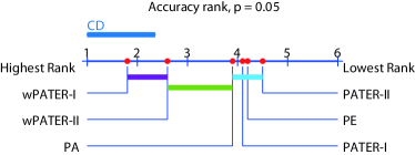
(a) Accuracy rank

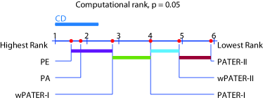
(b) Computational rank

Figure 2: The Nemenyi test to check statistical significance of the average (a) accuracies and (b) CPU times. The connected algorithms by the Critical Difference (CD) have no statistical significance.

5.2 Results and Discussion

Table 2 shows the average accuracies and its standard deviations on the 31 real-world data sets. Additionally, ranks for each algorithm are shown in brackets. In terms of the average accuracy, the proposed wPATER-I performs better accuracy performance than that of the other algorithms. Moreover, the proposed wPATER-II is also shown as the second best. In Table 2, both wPATER-I and wPATER-II achieve the best performances on the 29 data sets. In order to investigate the validity of the proposed wPATER for the data imbalance issue, in Table 3, we evaluate a best weight (BW), which gives the best accuracy, between $\alpha^{-}$ and $\alpha^{+}$ for each data set. We then present matching results between the best weights and needed weights (NW) which are given by the data imbalance ratios from Table 1. Consequently, Table 3 shows that our assumption of the proposed wPATER on addressing the data imbalance problems properly works in the 25 data sets. Figure 1 presents cumulative classification accuracies along the online learning process on the last 6 data sets (the data sets 26-31) that have large training samples. Except the ‘Ijcnn1’ data set in Figure 1(e), the PATER based algorithms maintain the best performers in terms of the cumulative accuracies. For time complexity, Table 4 shows the average CPU times on the aforementioned 31 data sets. In terms of the average CPU time, the proposed wPATER-I shows better CPU performance than that of the other algorithms.

To evaluate the statistical significance on the reported accuracy and CPU time comparisons, Friedman tests (see (Demšar, 2006)) and then Nemenyi plots are performed as a post-hoc test to statistically group connected algorithms at a confidence threshold (e.g., $p=0.05$). In terms of the accuracy rank, Fig. 2(a) has three groups of algorithms, namely 1) wPATER-I—wPATER-II, 2) wPATER-II—PA and 3) PA—PATER-I—PE—PATER-II. The proposed wPATER-I and wPATER-II are shown as the best group. In terms of the computational rank, Fig. 2(b) shows four groups of algorithms, namely 1) PE—PA—wPATER-I, 2) wPATER-I—PATER-I, 3) PATER-I—wPATER-II and 4) wPATER-II—PATER-II. The proposed wPATER-I is included in the best group, although this is shown as the third best individually. In summary, the proposed wPATER-I is seen as the best algorithm in terms of efficiency and effectiveness.

6 Conclusion

We have presented a passive-aggressive total-error-rate (PATER) minimization for online learning. Consequently, the proposed PATER had the useful properties of PA and TER together. In addition, a weighted PATER method (wPATER) has also presented to address the data imbalance problems. The proposed wPATER effectively and efficiently outperformed the state-of-the-art algorithms, including the proposed PATER on the real-world data sets. This work was based on the first-order information. We will improve this work to extend it to the second-order methods.

References

• Boyd & Vandenberghe (2004) Boyd, S. and Vandenberghe, L. Convex optimization. Cambridge University Press, 2004.
• Brodersen et al. (2010) Brodersen, K. H., Ong, C. S., Stephan, K. E., and Buhmann, J. M. The balanced accuracy and its posterior distribution. In International Conference on Pattern Recognition, pp. 3121–3124. IEEE, 2010.
• Cesa-Bianchi & Lugosi (2006) Cesa-Bianchi, N. and Lugosi, G. Prediction, learning, and games. Cambridge university press, 2006.
• Cesa-Bianchi et al. (2005) Cesa-Bianchi, N., Conconi, A., and Gentile, C. A second-order perceptron algorithm. SIAM Journal on Computing, 34(3):640–668, 2005.
• Chang & Lin (2011) Chang, C.-C. and Lin, C.-J. LIBSVM: A library for support vector machines. ACM Transactions on Intelligent Systems and Technology, 2:27:1–27:27, 2011. Software available at http://www.csie.ntu.edu.tw/~cjlin/libsvm.
• Crammer et al. (2006) Crammer, K., Dekel, O., Keshet, J., Shalev-Shwartz, S., and Singer, Y. Online passive-aggressive algorithms. Journal of Machine Learning Research, 7(Mar):551–585, 2006.
• Crammer et al. (2009) Crammer, K., Kulesza, A., and Dredze, M. Adaptive regularization of weight vectors. In Advances in neural information processing systems, pp. 414–422, 2009.
• Demšar (2006) Demšar, J. Statistical comparisons of classifiers over multiple data sets. Journal of Machine learning research, 7(Jan):1–30, 2006.
• Dredze et al. (2008) Dredze, M., Crammer, K., and Pereira, F. Confidence-weighted linear classification. In International Conference on Machine Learning, pp. 264–271. ACM, 2008.
• Hoi et al. (2018) Hoi, S. C. H., Sahoo, D., Lu, J., and Zhao, P. Online learning: A comprehensive survey. arXiv preprint arXiv:1802.02871, 2018.
• Lichman (2013) Lichman, M. UCI machine learning repository, 2013. URL http://archive.ics.uci.edu/ml.
• Rosenblatt (1958) Rosenblatt, F. The perceptron: A probabilistic model for information storage and organization in the brain. Psychological review, 65(6):386, 1958.
• Shalev-Shwartz (2011) Shalev-Shwartz, S. Online learning and online convex optimization. Foundations and Trends in Machine Learning, 4(2):107–194, 2011.
• Toh (2008) Toh, K.-A. Deterministic neural classification. Neural computation, 20(6):1565–1595, 2008.