Linking number of vortices as baryon number

Abstract

We show that the topological degree of a Skyrmion field is the same as the Hopf charge of the field under the Hopf map and thus equals the linking number of the preimages of two points on the 2-sphere under the Hopf map. We further interpret two particular points on the 2-sphere as vortex zeros and the linking of these zero lines follows from the latter theorem. Finally we conjecture that the topological degree of the Skyrmion can be interpreted as the product of winding numbers of vortices corresponding to the zero lines, summing over clusters of vortices.

1 Introduction

Skyrmions are topological solitons Manton:2004 of the texture type, i.e. they are maps from one-point compactified 3-space, $X=\mathbb{R}^{3}\cup\{\infty\}\simeq S^{3}$ to a target space $N=S^{3}$ with a nonvanishing topological degree $\pi_{3}(S^{3})=\mathbb{Z}\ni B\neq 0$. Usually the map is constructed using an SU(2) matrix $U$, where the nonlinear sigma model constraint is $\det U=1$, which forces the 4 components to live on a 3-sphere of unit radius. It is also possible to write the SU(2) matrix as an O(4) vector of unit length. In this paper, however, it proves convenient to write the SU(2) field as two complex scalar fields, $\psi_{1,2}$, living on the complexified 1-sphere ($|\psi_{1}|^{2}+|\psi_{2}|^{2}=1$). The convenience is two-fold. First of all, we would like to associate the zero lines of each complex scalar field with (deformed) vortex rings. Secondly, it proves convenient for our calculations as we will be using the Hopf map, which is naturally written in terms of two complex scalar fields.

First we prove a theorem which shows that under the Hopf map, the map $\boldsymbol{\psi}:\mathbb{R}^{3}\cup\{\infty\}\simeq S^{3}\to S^{3}$ of degree $B$ will necessarily have Hopf charge $Q=B$. This statement is known in the literature Ward:2001vi ; Manton:2004 and has been used several times to generate initial conditions for Hopfions Battye:1998pe ; Battye:1998zn in a different model, called the Faddeev-Skyrme model Faddeev:1996zj , which maps $\mathbb{R}^{3}$ to $S^{2}$ and thus naturally possesses a Hopf charge. Nevertheless, we have not found the theorem written down in the literature, and thus we shall give it here and supply a proof.

The implication of the theorem is that 2 distinct regular points under the projection of a Skyrme map to the 2-sphere have preimages in 3-space with linking number $Q=B$. We further make the interpretation of two antipodal points on the 2-sphere being vortex zeros. So far all is done with rigor. Finally, we conjecture that we can interpret the topological degree of a Skyrmion map as the product of winding numbers of two vortex lines, summing over clusters of wound vortices.

This paper is organized as follows. In sec. 2, after giving the maps, we present our theorem, corollary and conjecture. In sec. 3, we illustrate the theorem and conjecture with examples of a toroidal vortex and rational map Skyrmions. Sec. 4 is devoted to discussion and outlook.

2 The maps

2.1 Theorem and conjecture

We begin with considering a map from $U:X\to N$ where $X=\mathbb{R}^{3}\cup\,\{\infty\}\simeq S^{3}$ the one-point compactified 3-dimensional configuration space and $N=S^{3}$ is the target space, which we take to be the 3-sphere in this paper. Each space has an associated metric, that is $(X,g)$ and $(N,h)$. The map $U$ is characterized by the third homotopy group, $B\in\pi_{3}(S^{3})=\mathbb{Z}$ with $B$ the topological degree, which is usually called the baryon number.

Next, we will consider the Hopf map $H:S^{3}\to S^{2}$, which is due to the Hopf fibration $S^{1}\hookrightarrow S^{3}\overset{H}{\to}S^{2}$. The explicit form of the Hopf map is

$$H^{a}(\boldsymbol{\psi},\mkern 2.75mu\overline{\mkern-2.75mu\boldsymbol{\psi}\mkern-1.5mu}\mkern 1.5mu)=\boldsymbol{\psi}^{\dagger}\tau^{a}\boldsymbol{\psi},\qquad a=1,2,3,$$ (1)

with $\boldsymbol{\psi}$ living on the complexified 1-sphere:

$$\boldsymbol{\psi} =\begin{pmatrix}\psi_{1}\\ \psi_{2}\\ \end{pmatrix},\qquad\psi_{1,2}\in\mathbb{C},$$ (2)

$$\boldsymbol{\psi}^{\dagger}\boldsymbol{\psi}=|\psi_{1}|^{2}+|\psi_{2}|^{2}=1,$$ (3)

which is exactly a real 3-sphere and $\tau^{a}$ are the Pauli SU(2) matrices. The topological charge of the Hopf map is

$$Q\in\pi_{3}(S^{2}),$$ (4)

but it is not the degree of the mapping as it is a mapping between spaces of different dimensions.

The map $U:X\to N=S^{3}$ is given by

$$U(\mathbf{x})=\begin{pmatrix}\boldsymbol{\psi}&-\mathrm{i}\tau^{2}\mkern 2.75mu\overline{\mkern-2.75mu\boldsymbol{\psi}\mkern-1.5mu}\mkern 1.5mu\end{pmatrix}=\begin{pmatrix}\psi_{1}&-\mkern 2.75mu\overline{\mkern-2.75mu\psi\mkern-1.5mu}\mkern 1.5mu_{2}\\ \psi_{2}&\mkern 2.75mu\overline{\mkern-2.75mu\psi\mkern-1.5mu}\mkern 1.5mu_{1}\end{pmatrix},$$ (5)

which thus maps $\mathbb{R}^{3}\cup\{\infty\}=X\to S^{3}$, due to the constraint (3). The degree of the mapping $U$ from $X$ to $N$ can be calculated as the pullback of the normalized volume form on $N$, $\Omega_{N}$ by $U$:

$$B =\int_{X}U^{*}\Omega_{N}$$

$$=-\frac{1}{24\pi^{2}}\int_{X}{\rm tr}\,\left(U^{\dagger}\partial_{i}UU^{\dagger}\partial_{j}UU^{\dagger}\partial_{k}U\right){\mathrm{d}}{x}^{i}\wedge{\mathrm{d}}{x}^{j}\wedge{\mathrm{d}}{x}^{k}$$

$$=\frac{1}{4\pi^{2}}\int_{X}(\boldsymbol{\psi}^{\dagger}\partial_{i}\boldsymbol{\psi})(\partial_{j}\boldsymbol{\psi}^{\dagger}\partial_{k}\boldsymbol{\psi})\;{\mathrm{d}}{x}^{i}\wedge{\mathrm{d}}{x}^{j}\wedge{\mathrm{d}}{x}^{k}.$$ (6)

Finally, we are interested in the map $\boldsymbol{\phi}\equiv H\circ\,U:X\to S^{2}$, which is the composite map of $U$ and $H$. This takes a field configuration on $X$, maps it with degree $B$ to $N$ and then to $S^{2}$.

The Hopf charge (or Hopf index) of the above described map, $\boldsymbol{\phi}$, is given by Gladikowski:1996mb ; Faddeev:1996zj ,

$$Q=-\frac{1}{4\pi^{2}}\int_{X}A\wedge F,$$ (7)

where the field-strength tensor in terms of the coordinates on $S^{2}$ is Gladikowski:1996mb ; Faddeev:1996zj ,

$$F=\frac{1}{4}\boldsymbol{\phi}\cdot\partial_{i}\boldsymbol{\phi}\times\partial_{j}\boldsymbol{\phi}\;{\mathrm{d}}{x}^{i}\wedge{\mathrm{d}}{x}^{j},$$ (8)

and $A$ is a corresponding gauge field $F={\mathrm{d}}{A}$. However, it is not possible to write a local expression for the Chern-Simon action (7) in terms of the coordinates, $\boldsymbol{\phi}$, on $S^{2}$, because it vanishes identically, as well known.

Theorem 1.

A map $U:\mathbb{R}^{3}\cup\{\infty\}\to S^{3}$ with topological degree $B$ under the Hopf map $H:S^{3}\to S^{2}$ has Hopf charge $Q=B$ and thus distinct regular points on $S^{2}$ under the composite map $H\circ U:\mathbb{R}^{3}\cup\{\infty\}\to S^{2}$ have preimages on $\mathbb{R}^{3}\cup\{\infty\}$ that are linked $Q=B$ times.

Proof: We calculate the field-strength tensor (8) in terms of the coordinates on $S^{3}$ via the Hopf map (1) as

$$F =\frac{1}{4}\epsilon^{abc}(\boldsymbol{\psi}^{\dagger}\tau^{a}\boldsymbol{\psi})\partial_{i}(\boldsymbol{\psi}^{\dagger}\tau^{b}\boldsymbol{\psi})\partial_{j}(\boldsymbol{\psi}^{\dagger}\tau^{c}\boldsymbol{\psi})\;{\mathrm{d}}{x}^{i}\wedge{\mathrm{d}}{x}^{j}$$

$$=\mathrm{i}\left(\psi_{2}\mkern 2.75mu\overline{\mkern-2.75mu\psi\mkern-1.5mu}\mkern 1.5mu_{2}\partial_{i}\psi_{1}\partial_{j}\mkern 2.75mu\overline{\mkern-2.75mu\psi\mkern-1.5mu}\mkern 1.5mu_{1}-\psi_{2}\mkern 2.75mu\overline{\mkern-2.75mu\psi\mkern-1.5mu}\mkern 1.5mu_{1}\partial_{i}\psi_{1}\partial_{j}\mkern 2.75mu\overline{\mkern-2.75mu\psi\mkern-1.5mu}\mkern 1.5mu_{2}+\psi_{1}\mkern 2.75mu\overline{\mkern-2.75mu\psi\mkern-1.5mu}\mkern 1.5mu_{1}\partial_{i}\psi_{2}\partial_{j}\mkern 2.75mu\overline{\mkern-2.75mu\psi\mkern-1.5mu}\mkern 1.5mu_{2}-\psi_{1}\mkern 2.75mu\overline{\mkern-2.75mu\psi\mkern-1.5mu}\mkern 1.5mu_{2}\partial_{i}\psi_{2}\partial_{j}\mkern 2.75mu\overline{\mkern-2.75mu\psi\mkern-1.5mu}\mkern 1.5mu_{1}\right){\mathrm{d}}{x}^{i}\wedge{\mathrm{d}}{x}^{j}$$

$$=-\mathrm{i}\partial_{i}\boldsymbol{\psi}^{\dagger}\partial_{j}\boldsymbol{\psi}\;{\mathrm{d}}{x}^{i}\wedge{\mathrm{d}}{x}^{j},$$ (9)

where we have used the constraint (3). The above-calculated field-strength tensor can also readily be obtained from the following gauge field

$$A=-\frac{\mathrm{i}}{2}\left(\boldsymbol{\psi}^{\dagger}\partial_{i}\boldsymbol{\psi}-\partial_{i}\boldsymbol{\psi}^{\dagger}\boldsymbol{\psi}\right){\mathrm{d}}{x}^{i}.$$ (10)

We can now explicitly evaluate the Hopf charge (7) with the field-strength tensor (9) and the corresponding gauge field (10) and a simple calculation shows that it reduces to

$$Q=\frac{1}{4\pi^{2}}\int_{X}(\boldsymbol{\psi}^{\dagger}\partial_{i}\boldsymbol{\psi})(\partial_{j}\boldsymbol{\psi}^{\dagger}\partial_{k}\boldsymbol{\psi})\;{\mathrm{d}}{x}^{i}\wedge{\mathrm{d}}{x}^{j}\wedge{\mathrm{d}}{x}^{k},$$ (11)

which is exactly the same as the baryon charge (6). Since the baryon number $B$ (6) and the Hopf charge $Q$ (11) are given by the same integral expressions, then $B=Q$ follows. The final step is to use the fact that preimages of two distinct regular points on $S^{2}$ are linked $Q=B$ times under the Hopf map (1) and hence theorem 1 follows. $\square$

Now, if we pick any two regular (constant) points on $S^{2}$ as

$$\boldsymbol{\phi}_{1}\in S^{2},\qquad\boldsymbol{\phi}_{2}\in S^{2},$$ (12)

their preimages under the Hopf map composed with $U$, i.e. $\boldsymbol{\phi}=H\circ U$, have linking number $Q=B$. Since this holds for any two regular points, it also holds for the following case: Take the two points on $S^{2}$ to be

$$\boldsymbol{\phi}_{1}=H(\boldsymbol{\psi}_{1},\mkern 2.75mu\overline{\mkern-2.75mu\boldsymbol{\psi}\mkern-1.5mu}\mkern 1.5mu_{1})=(0,0,-1)^{\rm T},\qquad\boldsymbol{\phi}_{2}=H(\boldsymbol{\psi}_{2},\mkern 2.75mu\overline{\mkern-2.75mu\boldsymbol{\psi}\mkern-1.5mu}\mkern 1.5mu_{2})=(0,0,1)^{\rm T},$$ (13)

with

$$\boldsymbol{\psi}_{1}=\begin{pmatrix}0\\ 1\end{pmatrix},\qquad\boldsymbol{\psi}_{2}=\begin{pmatrix}1\\ 0\end{pmatrix}.$$ (14)

Any two regular points will have linking number $Q=B$; however, in order to interpret the preimages of the two points on $S^{2}$ as two vortex lines, we further need to require orthogonality

$$\boldsymbol{\psi}_{1}^{\dagger}\boldsymbol{\psi}_{2}=0,$$ (15)

which obviously holds for the two points in eq. (14).

Clearly it is possible that either both the points (13) or one of them are not regular points. Since the canonical mapping may not correspond to regular points under the Hopf map, we propose to rotate the 2-sphere until two regular points are found: $\boldsymbol{\phi}^{M}=M\boldsymbol{\phi}$ : $X\to S^{2}$ as

$$\boldsymbol{\phi}^{M}=MH(\boldsymbol{\psi},\bar{\boldsymbol{\psi}}).$$ (16)

The most general rotation of the 2-sphere can be done with three Euler angles and the following parametrization

$$M_{\alpha\beta\gamma} =M_{z}(\gamma)M_{x}(\beta)M_{z}(\alpha),$$ (17)

$$M_{z}(\alpha) =\begin{pmatrix}\cos\alpha&\sin\alpha&0\\ -\sin\alpha&\cos\alpha&0\\ 0&0&1\end{pmatrix},\qquad M_{x}(\beta)=\begin{pmatrix}1&0&0\\ 0&\cos\beta&\sin\beta\\ 0&-\sin\beta&\cos\beta\end{pmatrix}.$$ (18)

A particularly useful rotation brings the north and south poles to the equator of the 2-sphere:

$$M_{0\frac{\pi}{2}\gamma}=\begin{pmatrix}\cos\gamma&0&\sin\gamma\\ -\sin\gamma&0&\cos\gamma\\ 0&-1&0\end{pmatrix},$$ (19)

which yields a 1-parameter family of rotations of the north and south poles to the equator with angle $\gamma\in[0,2\pi)$:

$$\boldsymbol{\phi}_{1,2}^{M_{0\frac{\pi}{2}\gamma}}=M_{0\frac{\pi}{2}\gamma}\boldsymbol{\phi}_{1,2}=\mp\begin{pmatrix}\sin\gamma\\ \cos\gamma\\ 0\end{pmatrix},$$ (20)

where the upper sign corresponds to $\boldsymbol{\phi}_{1}$ and the lower sign $\boldsymbol{\phi}_{2}$.

Another useful rotation is

$$M_{0\beta 0}=M_{x}(\beta),$$ (21)

which yields a slightly different 1-parameter family of rotations

$$\boldsymbol{\phi}_{1,2}^{M_{0\beta 0}}=M_{0\beta 0}\boldsymbol{\phi}_{1,2}=\mp\begin{pmatrix}0\\ \sin\beta\\ \cos\beta\end{pmatrix},$$ (22)

where again the upper sign corresponds to $\boldsymbol{\phi}_{1}$ and the lower sign $\boldsymbol{\phi}_{2}$.

If we now take the parametrization of $\boldsymbol{\psi}$

$$\boldsymbol{\psi}=\begin{pmatrix}e^{\mathrm{i}\chi}\cos f\\ e^{\mathrm{i}\vartheta}\sin f\end{pmatrix},$$ (23)

we may interpret the two points, $\boldsymbol{\psi}_{1}$ and $\boldsymbol{\psi}_{2}$, of eq. (14) as the vortex zeros of the fields $\psi_{1}$ and $\psi_{2}$, respectively, see eq. (2). The composite map $\boldsymbol{\phi}:X\to S^{2}$ of eq. (23) thus reads

$$\boldsymbol{\phi}=\begin{pmatrix}\sin 2f\cos(\vartheta-\chi)\\ \sin 2f\sin(\vartheta-\chi)\\ \cos 2f\end{pmatrix},$$ (24)

from which it is clear that the two points $\boldsymbol{\phi}_{1,2}\in S^{2}$ of eq. (13) indeed are independent of $\vartheta$ and $\chi$ as they correspond to $f=\frac{\pi}{2}$ and $f=0$, respectively. These two vortex zeroes are canonically mapped to the south and north poles, respectively. Using now the rotated map $\boldsymbol{\phi}^{M_{0\frac{\pi}{2}\gamma}}$ of eq. (20), the vortex (23) is mapped to

$$\boldsymbol{\phi}^{M_{0\frac{\pi}{2}\gamma}}=\begin{pmatrix}\sin\gamma\cos 2f+\cos\gamma\sin 2f\cos(\vartheta-\chi)\\ \cos\gamma\cos 2f-\sin\gamma\sin 2f\cos(\vartheta-\chi)\\ -\sin 2f\sin(\vartheta-\chi)\end{pmatrix},$$ (25)

which at $f=\frac{\pi}{2},0$ equals eq. (20) by construction.

Corollary 1.

Two vortex lines (zeros), $\boldsymbol{\psi}_{1}$ and $\boldsymbol{\psi}_{2}$ of $\boldsymbol{\psi}\in X=\mathbb{R}^{3}\cup\{\infty\}$ are mapped to two distinct points on $S^{2}$ under the Hopf map $H\circ U:X\to S^{2}$ and hence their preimages in $X$ are linked $Q=B$ times due to theorem 1.

We may take a map $U:X\to N$ with topological degree $B$, project it onto $S^{2}$ with $H$ and select two regular points under the latter mapping

$$\boldsymbol{\phi}_{1,2}^{M_{0\frac{\pi}{2}\gamma}}=H\circ U,$$ (26)

where we have performed a rotation using eq. (20) and chosen an appropriate value for $\gamma$ such that the mapping is regular. Now due to the Corollary 1, we can follow the way back to $X$ with the inverse mappings and interpret the two points as vortex lines

$$\mathbf{x}_{1,2}(\tau,\ell)=(H\circ U)^{-1}\left(\boldsymbol{\phi}_{1,2}^{M_{0\frac{\pi}{2}\gamma}}\right),$$ (27)

which yields two vortex lines with some parametrization $\tau$ and we have included an index $\ell$ in case the preimages separate into several clusters.

We are now ready to make the following conjecture.

Conjecture 1.

A map $U:\mathbb{R}^{3}\cup\{\infty\}=X\to S^{3}$ having degree $B$ (6) can be interpreted as two vortices in $\psi_{1}$ and $\psi_{2}$ of $\boldsymbol{\psi}\in S^{3}$ which in each cluster topologically have winding numbers $p_{\ell}$ and $q_{\ell}$, respectively. Then due to Corollary 1, the linking number $Q$ (11) is $\sum_{\ell}p_{\ell}q_{\ell}$ and due to theorem 1, $B=Q=\sum_{\ell}p_{\ell}q_{\ell}$.

2.2 The rational map

We will now consider $U$ to be in a class of maps, where it is a radial suspension in $\mathbb{R}^{3}$ and the tangent directions are described by rational maps between Riemann spheres. The rational map Ansatz is given by

$$U=\exp\left(\mathrm{i}f(r)\mathbf{n}\cdot\mathbf{\tau}\right),$$ (28)

with

$$\mathbf{n}=\left(\frac{R+\mkern 2.75mu\overline{\mkern-2.75muR\mkern-1.5mu}\mkern 1.5mu}{1+|R|^{2}},\frac{\mathrm{i}(\mkern 2.75mu\overline{\mkern-2.75muR\mkern-1.5mu}\mkern 1.5mu-R)}{1+|R|^{2}},\frac{1-|R|^{2}}{1+|R|^{2}}\right),$$ (29)

where $R=R(z)$ is a holomorphic function of the Riemann sphere coordinate $z=e^{\mathrm{i}\phi}\tan\tfrac{\theta}{2}$ and $(r,\theta,\phi)$ are standard spherical coordinates in $\mathbb{R}^{3}$.

Using eq. (5), we get

$$\boldsymbol{\psi}=\frac{1}{1+|R|^{2}}\begin{pmatrix}e^{\mathrm{i}f}+|R|^{2}e^{-\mathrm{i}f}\\ \mathrm{i}2R\sin f\end{pmatrix},$$ (30)

which we map to the 2-sphere using $H$ of eq. (1), yielding

$$\boldsymbol{\phi}=\frac{1}{(1+|R|^{2})^{2}}\begin{pmatrix}-2\Im(R)(1+|R|^{2})\sin 2f+4\Re(R)(1-|R|^{2})\sin^{2}f\\ 2\Re(R)(1+|R|^{2})\sin 2f+4\Im(R)(1-|R|^{2})\sin^{2}f\\ 4|R|^{2}\cos 2f+(1-|R|^{2})^{2}\end{pmatrix}.$$ (31)

It is easy to check that the above $\boldsymbol{\phi}$ is a real-valued 3-vector of unit norm, thus living on $S^{2}$. One can also readily verify that $f=\frac{\pi}{2},0$ correspond to $\boldsymbol{\phi}_{1,2}$, respectively.

3 Examples

3.1 Toroidal vortex

Let us consider a simple example inspired by ref. Gudnason:2016yix ; Gudnason:2014gla ; Gudnason:2014hsa ; Gudnason:2014jga ; Gudnason:2018oyx where a vortex ring is twisted $P$ times, yielding baryon number $P$:

$$\boldsymbol{\psi}=\begin{pmatrix}\cos f(r)+\mathrm{i}\sin f(r)\cos\theta\\ \sin f(r)\sin\theta e^{\mathrm{i}P\phi}\end{pmatrix}.$$ (32)

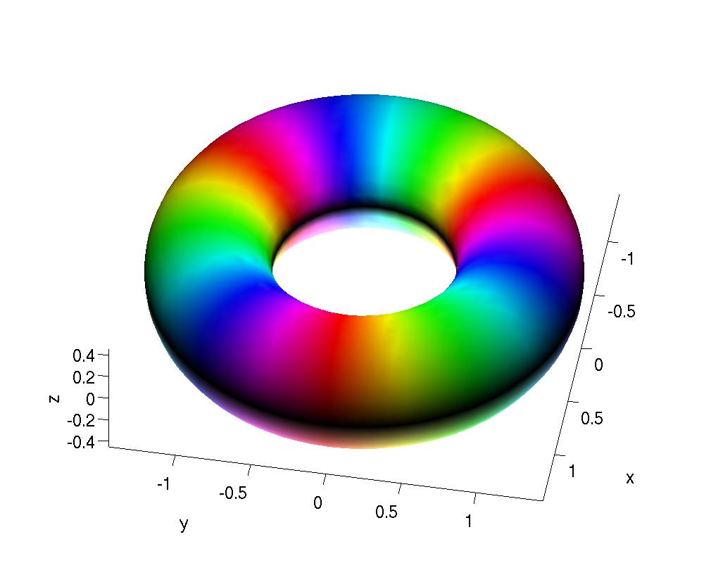
Figure 1: Vortex ring with $P=3$ twists. Figure taken from ref. Gudnason:2014jga .

The energy functional that gives rise to toroidal vortices is given by Gudnason:2016yix

$$E[\boldsymbol{\psi}]=\|{\mathrm{d}}\boldsymbol{\psi}\|_{L^{2}(X)}^{2}+\frac{1}{4}\|\boldsymbol{\psi}^{*}{\mathrm{d}}{\mu}\|_{L^{2}(X)}^{2}+\int_{X}*V(\boldsymbol{\psi}),\qquad V(\boldsymbol{\psi})=\frac{m^{2}}{2}(1-|\psi_{1}|^{2}),$$ (33)

where $\mu$ is the Maurer-Cartan form on $N$ (SU(2)) and the second term is the norm-squared of the pullback of the exterior derivative of the Maurer-Cartan form on $N$ by $\boldsymbol{\psi}$. $m$ is a positive constant which must be large enough $m>m_{\rm crit}$. Finally $*$ denotes the Hodge dual such that $*1$ gives the volume form (and in this case on $X$). The baryon charge density isosurface is shown in fig. 1, which is taken from ref. Gudnason:2014jga where further details can be found. It is easy to check that the topological degree (6) is given by

$$B =-\frac{P}{\pi}\int_{0}^{\pi}\sin\theta\,{\mathrm{d}}{\theta}\int_{0}^{\infty}\sin^{2}f(r)\partial_{r}f(r)\,{\mathrm{d}}{r}$$

$$=-\frac{P}{2\pi}\left[2f(r)-\sin 2f(r)\right]_{f(0)}^{f(\infty)}$$

$$=P,$$ (34)

where we have used the boundary conditions $f(0)=\pi$ and $f(\infty)=0$.

Under the map (1) we have

$$\boldsymbol{\phi}=\begin{pmatrix}\sin\theta\cos P\phi\sin 2f(r)+\sin 2\theta\sin P\phi\sin^{2}f(r)\\ \sin\theta\sin P\phi\sin 2f(r)-\sin 2\theta\cos P\phi\sin^{2}f(r)\\ \sin^{2}\theta\cos 2f(r)+\cos^{2}\theta\end{pmatrix}.$$ (35)

An obvious choice would be to pick the two points $\boldsymbol{\phi}_{1,2}$ of eq. (13) on the 2-sphere, yielding

$$\cos^{2}f=\cos^{2}\theta =0,\qquad(\boldsymbol{\phi}=\boldsymbol{\phi}_{1},\;\psi_{1}=0)$$ (36)

$$\sin^{2}f\sin^{2}\theta =0,\qquad(\boldsymbol{\phi}=\boldsymbol{\phi}_{2},\;\psi_{2}=0).$$ (37)

Let us start with the latter equation; $\sin f=0$ corresponds to the vacuum at $r\to\infty$ and the origin where $f=\pi$. Hence in the interior of $\mathbb{R}^{3}\backslash\{0\}$, $\sin f\neq 0$ and thus $\sin\theta=0$ corresponds to the $x^{3}$ axis. We call it a “vacuum vortex,” specified by $\psi_{2}=0$. On $X\simeq S^{3}$ this is topologically a circle ($S^{1}$) going from the north pole of the 3-sphere (the vacuum) from $x^{3}=-\infty$ to the origin $\mathbf{x}=\mathbf{0}$ which is the south pole of the 3-sphere, and then towards $x^{3}\to+\infty$ back to north pole. The former equation has two conditions yielding $\theta=\frac{\pi}{2}$ and $f(r)=\frac{\pi}{2}$, which is a circle in the $(x^{1},x^{2})$-plane, representing a ring-shaped “physical” vortex specified by $\psi_{1}=0$. This obviously yields a linking number equal to 1. Although this is a natural interpretation of where the two vortices might be in this field configuration, $\boldsymbol{\phi}_{2}$ is not a regular point of the mapping when $P>1$.

    

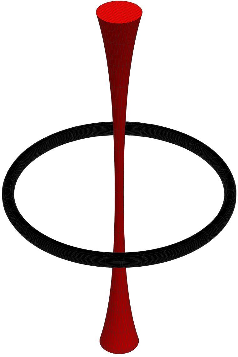
(a) $\beta=0$

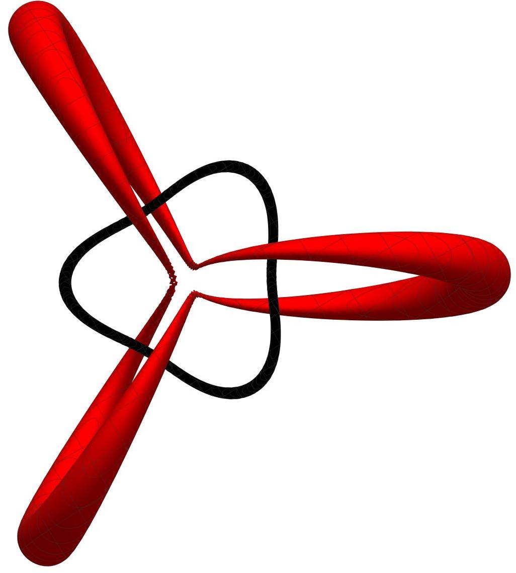
(b) $\beta=\frac{\pi}{6}$

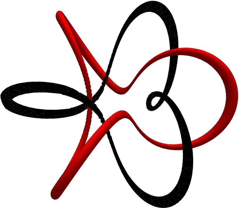
(c) $\beta=\frac{\pi}{2}$

Figure 2: The toroidal vortex (black) with $P=3$ twists and its vacuum vortex (red) at rotation angles $\beta=0,\frac{\pi}{6},\frac{\pi}{2}$. The angle $\beta=0$ corresponds to no rotation and shows the degeneracy of the vacuum vortex which is due to the north pole on the 2-sphere not being a regular point under the Hopf map.

In order to move away from the point where the $P$ vortices linking the “vacuum vortex” are degenerate, we pick two points on the 2-sphere after a rotation by an angle $\beta$:

$$\boldsymbol{\phi}_{1,2}^{M_{0\beta 0}},$$ (38)

with $M_{\alpha\beta\gamma}$ given by eq. (17) and $\boldsymbol{\phi}_{1,2}$ given by eq. (13). The expression is not particularly illuminating, so we will just plot the preimages of the two points on the rotated 2-sphere in fig. 2.

Plotting the preimage of one of the points on the 2-sphere amounts to finding the solutions to the inverse map

$$\mathbf{x}=\boldsymbol{\phi}^{-1}(\boldsymbol{\phi}_{a}),$$ (39)

with $\boldsymbol{\phi}_{a}$ a chosen point on $S^{2}\ni\boldsymbol{\phi}_{a}=\boldsymbol{\phi}(\mathbf{x})$. In practice, the solution to this problem is a hairline and not easy to see on a 3-dimensional graph, so we plot instead a surface that corresponds to 1% of the neighborhood around $\boldsymbol{\phi}_{a}$. In particular, if we want to plot $\mathbf{x}=\boldsymbol{\phi}^{-1}((0,0,-1))$, we instead plot the surface $\boldsymbol{\phi}^{-1}\big{(}(a,b,-\sqrt{1-a^{2}-b^{2}})\big{)}$ with $\sqrt{a^{2}+b^{2}}=0.01$.

Fig. 2(a) shows the unrotated degenerate case, where the vacuum vortex with winding number 3 is coincident – this thus corresponds to a point on the 2-sphere which is not regular under the Hopf map (1). In fig. 2(b) we have increased $\beta$ to $\beta=\frac{\pi}{6}$ and we have moved away from the degeneracy of the vacuum vortex. Now we can clearly see that the vortex ring, which is the black circle depicted in fig. (2)(a), is linked 3 times with the vacuum vortex (red). Note that both preimages are themselves not knots, but indeed unknots.

A comment in store is about the black line, i.e. the vortex ring itself in fig. 2. In fig. 2(a) the preimage shows the center of the vortex and what one normally would associate with the position of the vortex; unfortunately the antipodal point on the 2-sphere under the Hopf map is not regular, as mentioned above. Once we rotate the two points, $\boldsymbol{\phi}_{1,2}$, keeping them antipodal on the 2-sphere, we also move the vortex point itself and the preimage runs $P$ times around the vortex center line on fixed level sets of the vortex field. At the $\beta=\frac{\pi}{2}$ rotation, we have rotated all the way to the equator, which corresponds to $\gamma=0$ of eq. (20). Here the vortex line and the vacuum vortex becomes identical, except that one is rotated by $\pi/P=\pi/3$ with respect to the other.

This example thus confirms conjecture 1 with the vortex ring having $q=1$ and the vacuum vortex having $p=3$, yielding $B=Q=pq=3$.

Before moving on to the next example, let us make one more comment. The energy (33) is an example where the potential term is asymmetric in $\psi_{1}$ and $\psi_{2}$, so the physical vortex zeros correspond to $\psi_{1}=0$ and the vacuum vortex zeros to $\psi_{2}=0$. Instead, we could consider the potential term which is symmetric in $\psi_{1}$ and $\psi_{2}$ Gudnason:2014gla ; Gudnason:2014hsa ; Gudnason:2014jga ; Gudnason:2018oyx

$$V(\boldsymbol{\psi})=\pm\frac{m^{2}}{8}\big{[}1-(\boldsymbol{\psi}^{\dagger}\sigma_{3}\boldsymbol{\psi})^{2}\big{]}=\pm\frac{m^{2}}{2}|\psi_{1}|^{2}|\psi_{2}|^{2}.$$ (40)

For the positive sign, there are two vacua: $\boldsymbol{\psi}=(e^{\mathrm{i}\alpha},0)$ and $(0,e^{\mathrm{i}\alpha})$ Gudnason:2014gla ; Gudnason:2014hsa ; Gudnason:2014jga ; Gudnason:2018oyx , while for the negative sign the vacuum is: $S^{1}\times S^{1}$, $|\psi_{1}|^{2}=|\psi_{2}|^{2}=1/2$. In the former case, the situation is similar to that of the potential (33) admitting physical vortex zeros and vacuum vortex zeros, while in the latter case both zeros can be physical vortices. This potential is motivated by two-component Bose-Einstein condensates (BEC) Kasamatsu , and we called the model the BEC-Skyrme model, see Appendix A of ref. Gudnason:2014hsa for a more precise correspondence. In fact, a Skyrmion in two-component BECs was constructed as a link of two kinds of vortices Ruostekoski:2001fc ; Battye:2001ec ; Nitta:2012hy .

3.2 Rational map Skyrmions

We will now illustrate theorem 1 and conjecture 1 using the rational map approximation to Skyrmion solutions Houghton:1997kg . The energy functional is now simply given by

$$E[\boldsymbol{\psi}]=\|{\mathrm{d}}\boldsymbol{\psi}\|_{L^{2}(X)}^{2}+\frac{1}{4}\|\boldsymbol{\psi}^{*}{\mathrm{d}}{\mu}\|_{L^{2}(X)}^{2},$$ (41)

see the previous subsection for an explanation. Inserting the rational map Ansatz (28) yields

$$E[f,R]=\int_{0}^{\infty}\left(f^{{}^{\prime}2}+2B\sin^{2}f(f^{{}^{\prime}2}+1)+\mathcal{I}[R]\frac{\sin^{4}f}{r^{4}}\right)r^{2}\;{\mathrm{d}}{r},$$ (42)

with

$$\mathcal{I}[R]=\frac{1}{4\pi}\|R^{*}\Omega_{N}\|_{L^{2}(S^{2})}^{2},$$ (43)

where the only way the rational map enters the energy functional is through this integral which is the norm-squared of the pullback of the area form on $N$ by $R$, and $B$ is the degree of the rational map $R$.

We will thus utilize the map (31) with $R(z)$ being the rational map of degree $B$. Plotting the points (13) corresponds to a vortex (which is the antivacuum of the Skyrmion) and the vacuum vortex (which contains the vacuum). In all cases, except the $B=1$ case, the vacuum vortex does not correspond to a regular point under the map (31) and hence the preimages degenerate, making it impossible to count the linking number – which indeed is in accord with theorem 1. For certain $B$, even the vortex (the antivacuum) does not correspond to a regular point under the mapping. Therefore, we turn to (two) antipodal points on the 2-sphere, which do correspond to regular points under the map (31) by rotating the 2-sphere using eqs. (20), (22) and the linking numbers thus exactly equal the baryon numbers of the solitons.

In order to facilitate the visualization of the preimages of the soliton solutions in terms of Skyrmion maps, it will prove helpful to plot a fixed level set of the baryon charge density so as to get a frame of reference for the preimages. The baryon charge density is given by

$$\mathcal{B}=*\boldsymbol{\psi}^{*}\Omega_{N},$$ (44)

which is a 0-form (scalar quantity) and is calculated as the Hodge dual on $X$ of the pullback of the normalized volume form on $N$ by the map $\boldsymbol{\psi}$.

We are now ready to present the results of various preimages of the points $\boldsymbol{\phi}_{1,2}^{M_{0\frac{\pi}{2}\gamma}}$ and $\boldsymbol{\phi}_{1,2}^{M_{0\beta 0}}$ for rational map Skyrmions with $B=1,2,\ldots,8$. We will display the degenerate points $\boldsymbol{\phi}_{1,2}$ just for reference.

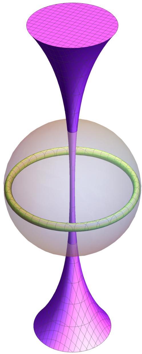
(a) $\boldsymbol{\phi}_{1,2}$

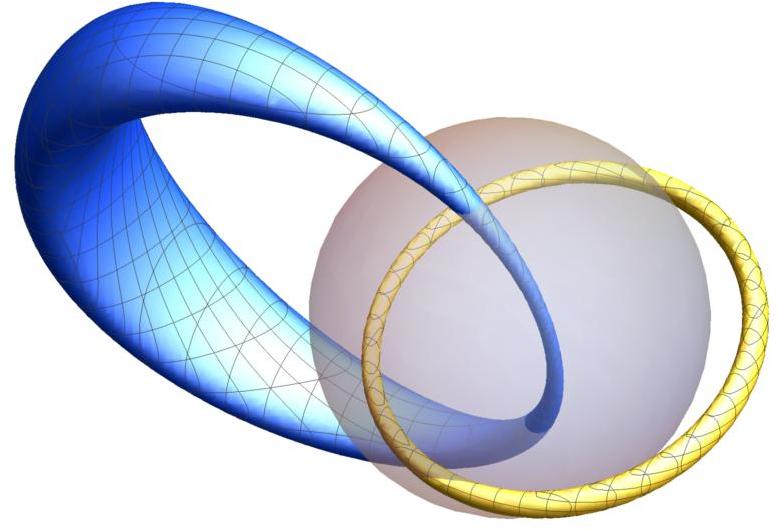
(b) $\boldsymbol{\phi}_{1,2}^{M_{0\frac{\pi}{2}\frac{\pi}{4}}}$

Figure 3: Links for the $B=1$ Skyrmion. (a) A link between the vortex ring (yellow) and the vacuum vortex (magenta). (b) A link between the vortex (yellow) and the vacuum vortex (blue) which is a closed loop. The gray isosurface is the baryon charge density illustrating the shape of the Skyrmion.

The rational map Skyrmion with topological degree 1 is given by the spherically symmetric rational map Houghton:1997kg

$$R_{1}(z)=z.$$ (45)

Fig. 3 shows the preimages of $\boldsymbol{\phi}_{1,2}$ and again after a rotation using the rotation matrix $M_{0\frac{\pi}{2}\frac{\pi}{4}}$ of eq. (20) has been applied. In this case, and only in this case, $\boldsymbol{\phi}_{1,2}$ are regular points under the mapping (31). The vacuum vortex (magenta) in fig. 3(a) goes from $x^{3}=-\infty$ to $x^{3}=\infty$, which are identified by the one-point compactification and hence it is a vortex ring, linking the other vortex ring (yellow) exactly once, as expected.

In order to see what happens to the preimages once the rotation of the 2-sphere has been applied, we show $\boldsymbol{\phi}_{1,2}^{M_{0\frac{\pi}{2}\frac{\pi}{4}}}$ in fig. 3(b). The two points are still antipodal on the 2-sphere in order to lend the interpretation as “vortices,” but it is clear that the vortex (yellow) is slightly shifted and the vacuum vortex (blue) is now closing in the bulk of $\mathbb{R}^{3}$. Topologically it is the same thing of course and since both points are regular, they both give linking number $Q=B=1$ as theorem 1 states and the interpretation as vortex links according to conjecture 1 is also clear.

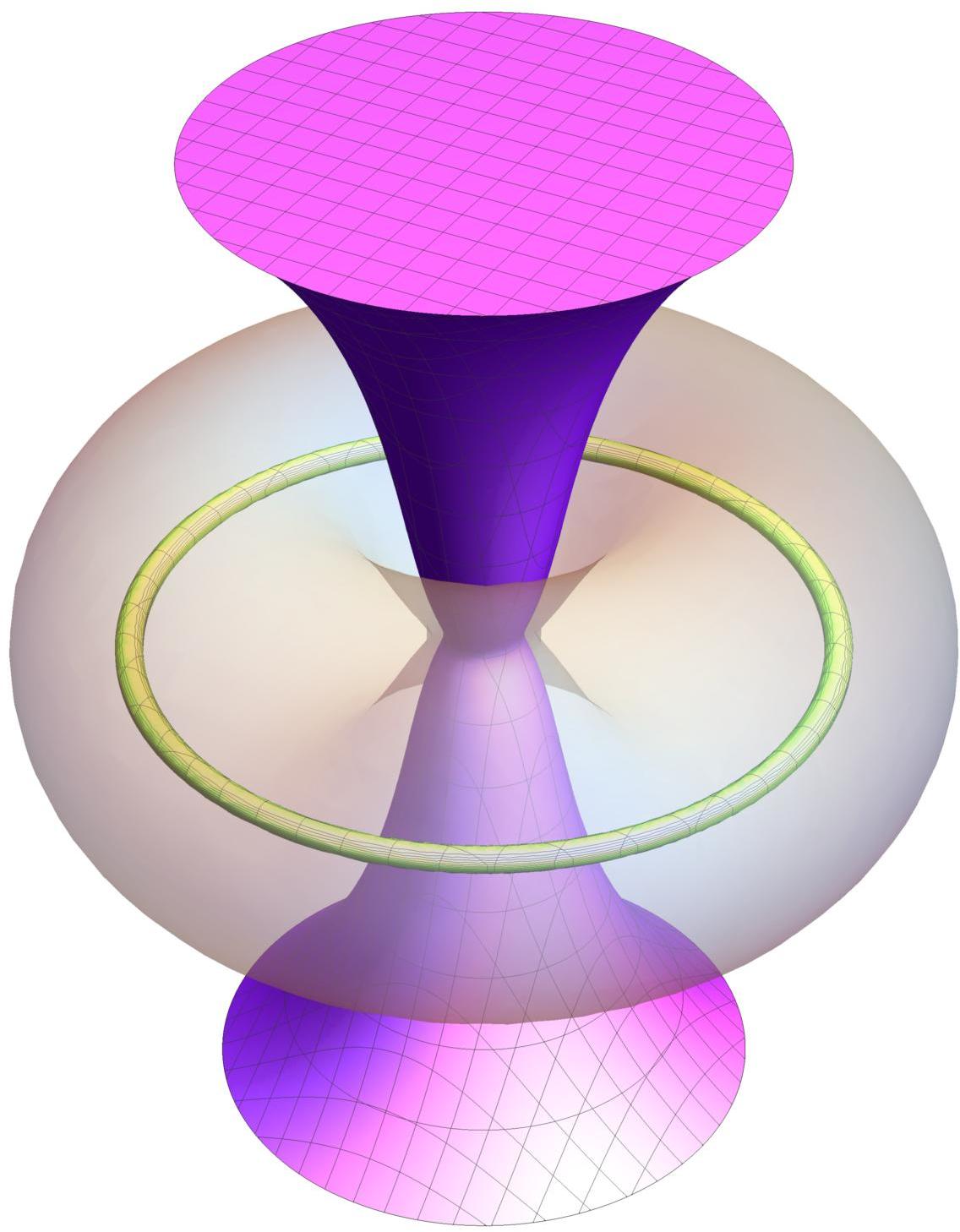
(a) $\boldsymbol{\phi}_{1,2}$

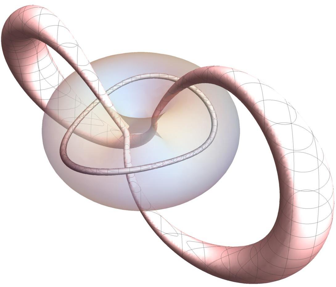
(b) $\boldsymbol{\phi}_{1,2}^{M_{0\frac{\pi}{6}0}}$

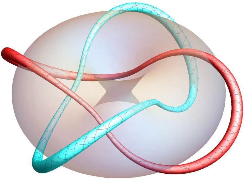
(c) $\boldsymbol{\phi}_{1,2}^{M_{0\frac{\pi}{2}0}}$

Figure 4: Links for the $B=2$ Skyrmion. (a) A link between the vortex ring (yellow) and the vacuum vortex (magenta) which is degenerate. (b,c) Nondegenerate links between the vortex and vacuum vortex, which are both closed loops. The gray isosurface is the baryon charge density illustrating the shape of the Skyrmion.

The rational map Skyrmion with topological degree 2 is given by the axially symmetric rational map Houghton:1997kg

$$R_{2}(z)=z^{2}.$$ (46)

Fig. 4 shows preimages of $\boldsymbol{\phi}_{1,2}$ and again after a rotation by $\beta=\frac{\pi}{6}$ and $\beta=\frac{\pi}{2}$. The vacuum vortex (magenta) in fig. 4(a) is degenerate and this is because the point on the 2-sphere is not a regular point under the mapping (31), as mentioned already. Rotating the points, keeping them mutually antipodal, the preimages of fig. 4(b) are perfectly linked twice and in fig. 4(c) the vacuum vortex becomes identical with the vortex, albeit with a $\pi/2$ rotation with respect to the latter. This example confirms conjecture 1 with the vortex ring having $q=1$ and the vacuum vortex having $p=2$, yielding $B=Q=pq=2$.

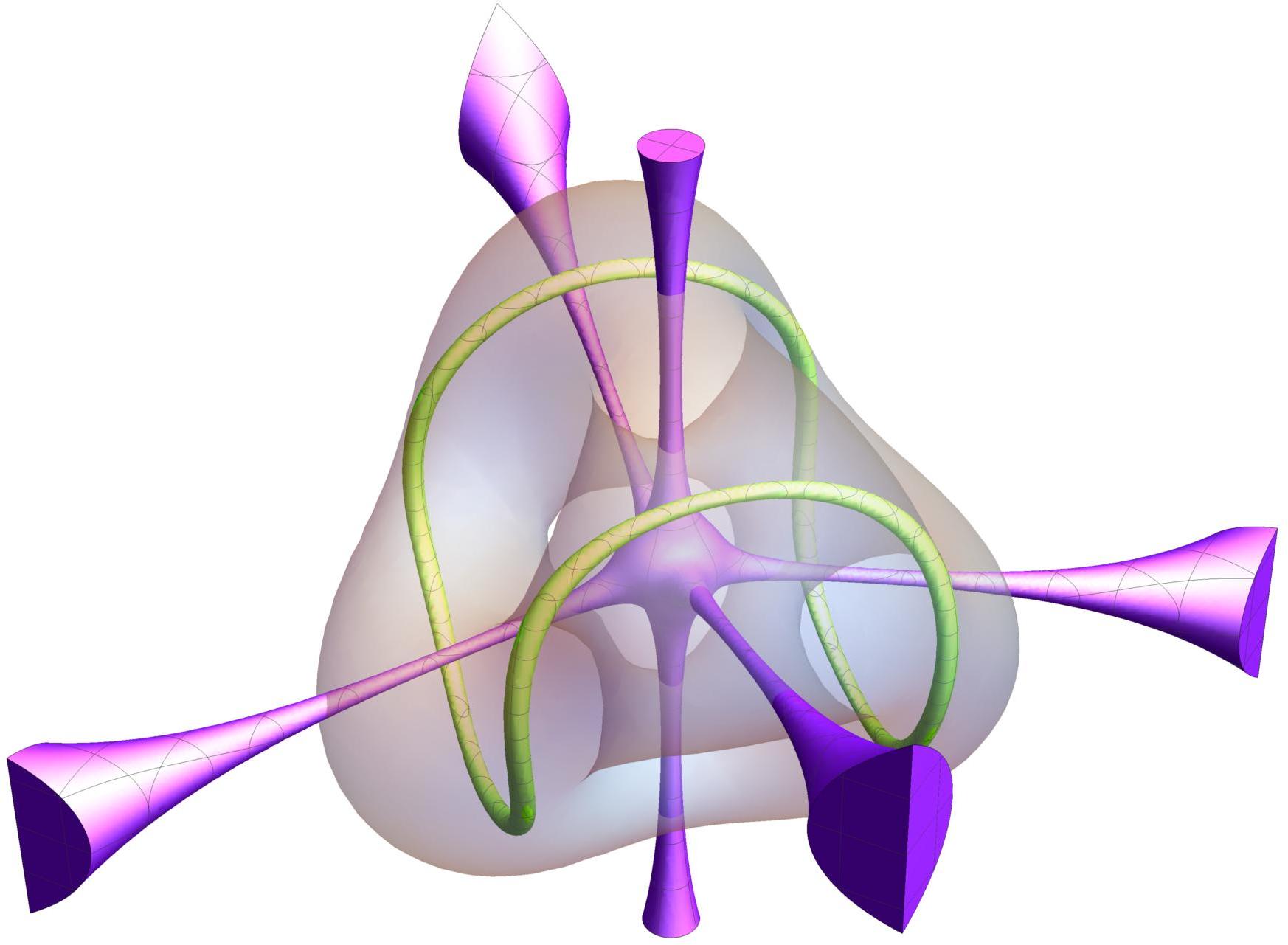
(a) $\boldsymbol{\phi}_{1,2}$

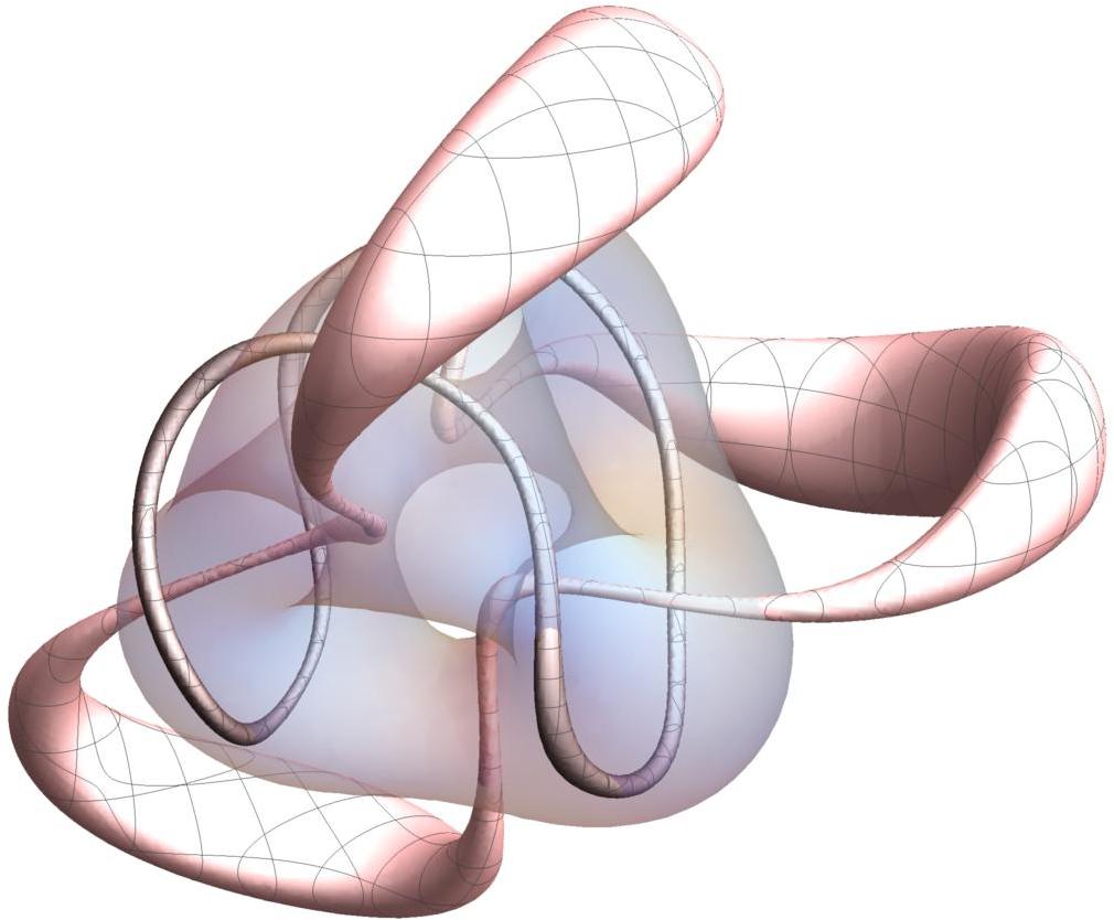
(b) $\boldsymbol{\phi}_{1,2}^{M_{0\frac{\pi}{6}0}}$

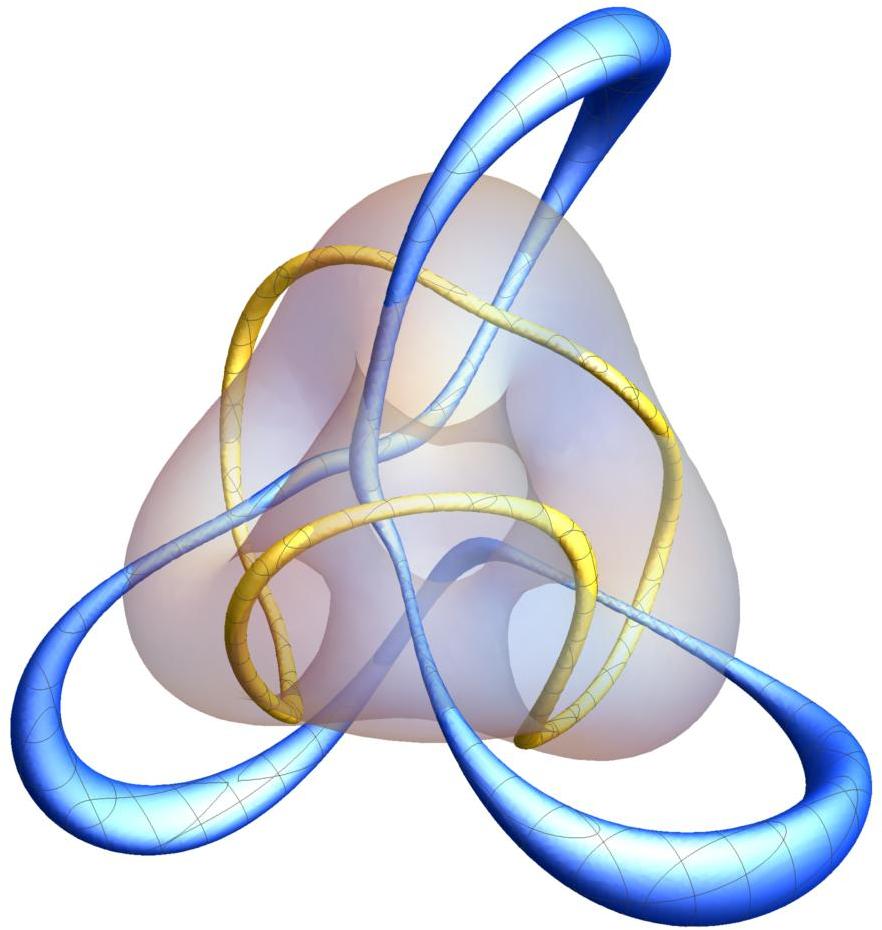
(c) $\boldsymbol{\phi}_{1,2}^{M_{0\frac{\pi}{2}\frac{\pi}{4}}}$

Figure 5: Links for the $B=3$ Skyrmion. (a) A link between the vortex ring (yellow) and the vacuum vortex (magenta) which is degenerate. (b,c) Nondegenerate links between the vortex and vacuum vortex, which are both closed loops. The gray isosurface is the baryon charge density illustrating the shape of the Skyrmion.

The next soliton is the rational map Skyrmion of topological degree 3. The rational map is given by Houghton:1997kg

$$R_{3}(z)=\frac{\mathrm{i}\sqrt{3}z^{2}-1}{z(z^{2}-\mathrm{i}\sqrt{3})},$$ (47)

and possesses tetrahedral symmetry. Fig. 5 shows preimages of $\boldsymbol{\phi}_{1,2}$ as well as two rotations by $\beta=\frac{\pi}{6}$ and by $\gamma=\frac{\pi}{4}$. The vacuum vortex (magenta) in fig. 5(a) is still degenerate as mentioned above. There is now evidence for the vacuum vortex of rational map Skyrmions to be $B$ intersecting (infinite) lines coming from and returning to $\partial\mathbb{R}^{3}$. After a suitable rotation as shown in fig. 5(b,c) the linking number of two antipodal points on the 2-sphere is now equal to three, as promised. This example confirms conjecture 1 with the vortex ring having $q=1$ and the vacuum vortex having $p=3$, yielding $B=Q=pq=3$.

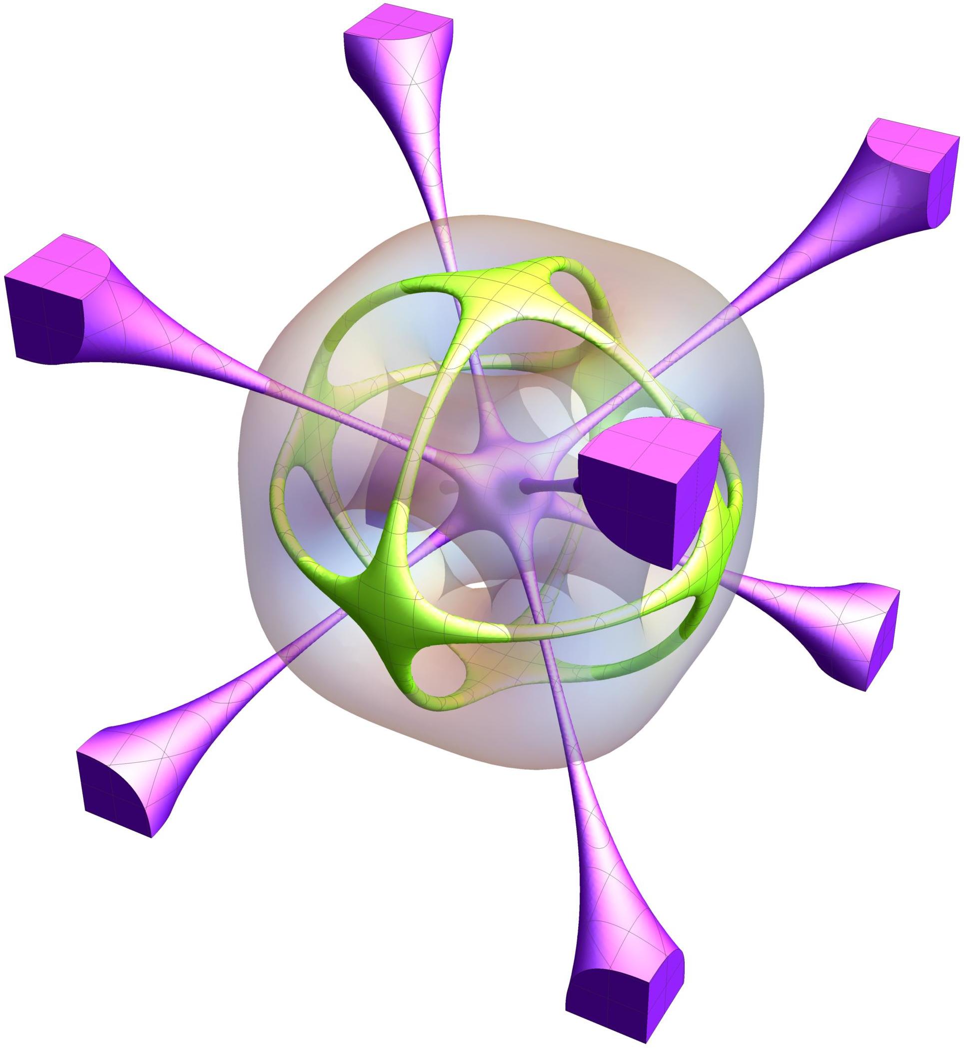
(a) $\boldsymbol{\phi}_{1,2}$

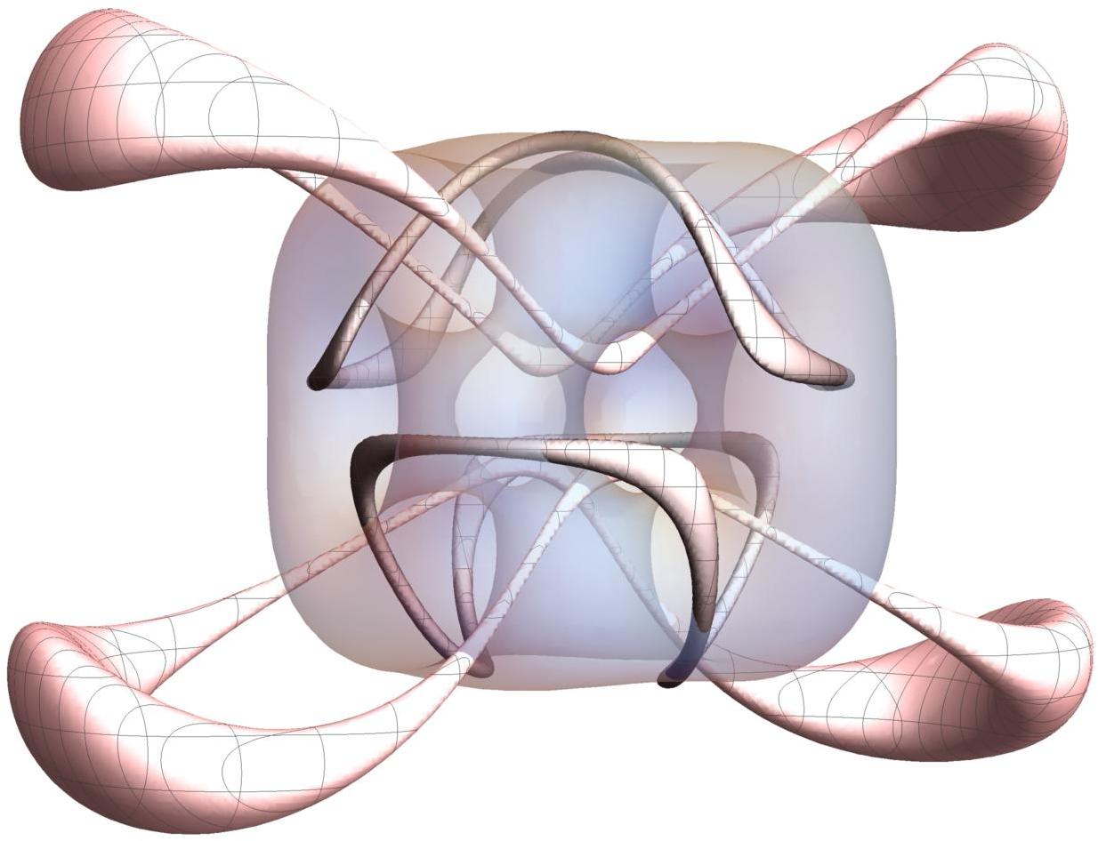
(b) $\boldsymbol{\phi}_{1,2}^{M_{0\frac{\pi}{6}0}}$

(c) $\boldsymbol{\phi}_{1,2}^{M_{0\frac{3\pi}{2}0}}$

Figure 6: Links for the $B=4$ Skyrmion. (a) A link between the vortex ring (yellow) and the vacuum vortex (magenta), which are both degenerate. (b,c) Nondegenerate links between the vortices and vacuum vortices, which are both closed loops. The gray isosurface is the baryon charge density illustrating the shape of the Skyrmion.

The $B=4$ Skyrmion has octahedral symmetry, which is the dual symmetry of the cube, and the rational map with such symmetry reads Houghton:1997kg

$$R_{4}(z)=\frac{z^{4}+\mathrm{i}2\sqrt{3}z^{2}+1}{z^{4}-\mathrm{i}2\sqrt{3}z^{2}+1}.$$ (48)

Fig. 6 shows preimages of $\boldsymbol{\phi}_{1,2}$ as well as two rotations thereof, by $\beta=\frac{\pi}{6}$ and by $\beta=\frac{3\pi}{2}$. As for all $B>1$, the vacuum vortex (magenta) in fig. 6 is degenerate, but this time also the vortex or antivacuum (yellow) is degenerate with merging points of the curves at each face of the cube. Rotating the vortex points by $\beta=\frac{\pi}{6}$ and by $\beta=\frac{3\pi}{2}$, see fig. 6(b,c), yields regular points on the 2-sphere under the mapping and the links are clear. This time, however, the linking number is split into two disjoint clusters of links and the total linking number is given by $q_{1}=1$, $p_{1}=2$, $q_{2}=1$, $p_{2}=2$ and hence $B=Q=\sum_{\ell=1}^{2}p_{\ell}q_{\ell}=4$, as promised. This example confirms conjecture 1 and this time with 2 clusters adding up to the total linking number.

An interesting note is that one can see the structure of the $B=4$ cubic Skyrmion being composed by two tori, with one of them flipped with respect to the other.

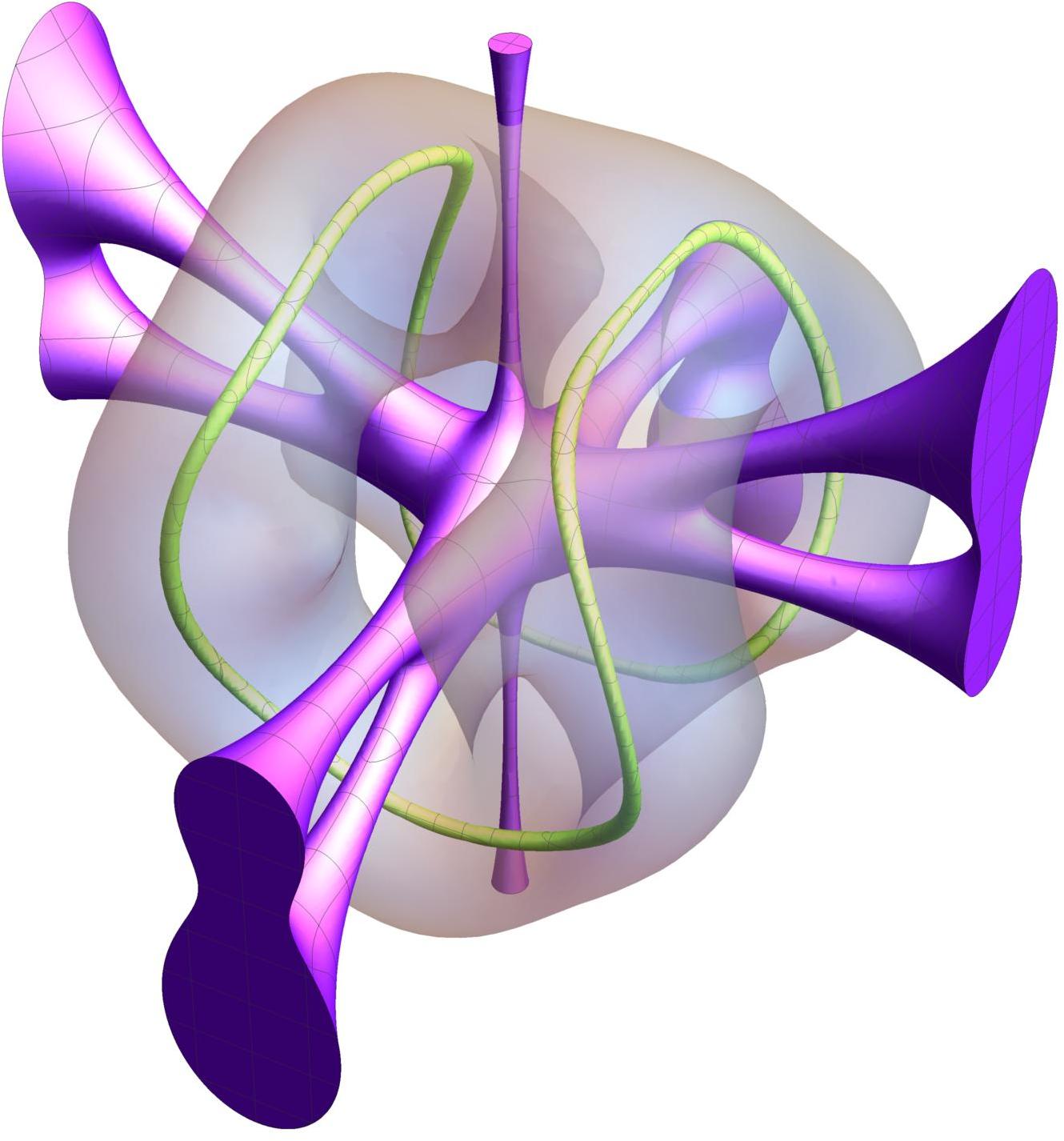
(a) $\boldsymbol{\phi}_{1,2}$

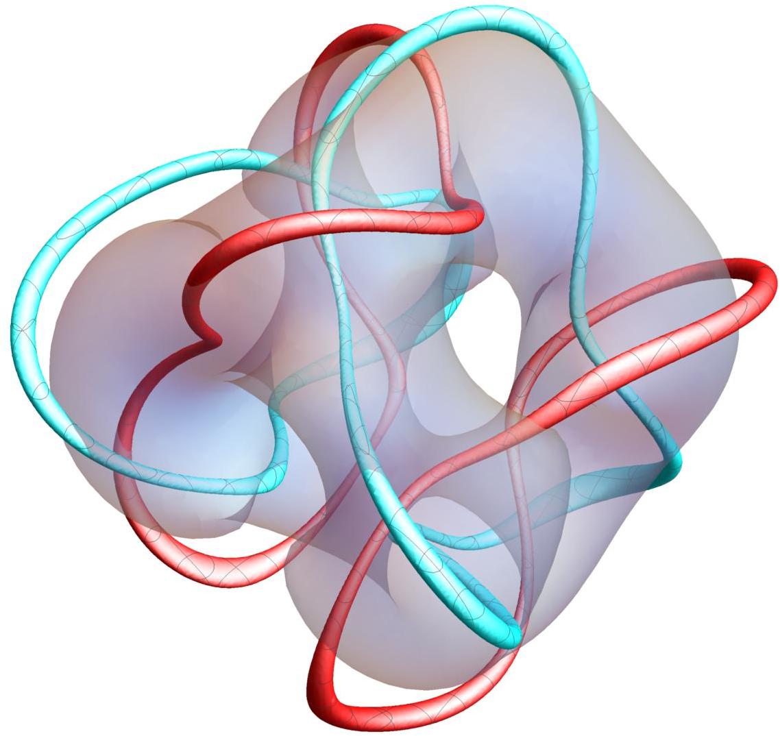
(b) $\boldsymbol{\phi}_{1,2}^{M_{0\frac{\pi}{2}0}}$

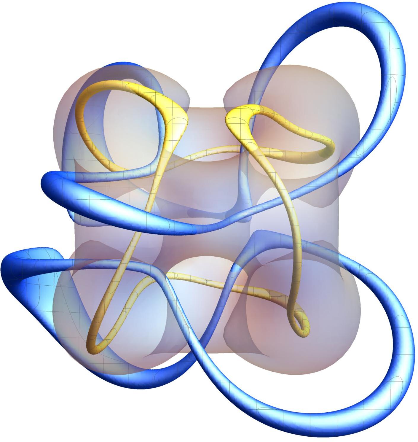
(c) $\boldsymbol{\phi}_{1,2}^{M_{0\frac{\pi}{2}\frac{\pi}{4}}}$

Figure 7: Links for the $B=5$ Skyrmion. (a) A link between the vortex ring (yellow) and the vacuum vortex (magenta) which is degenerate. (b,c) Nondegenerate links between the vortices and vacuum vortices, which are both closed loops. The gray isosurface is the baryon charge density illustrating the shape of the Skyrmion.

The $B=5$ Skyrmion has dihedral ($D_{2d}$) symmetry and the corresponding rational map is Houghton:1997kg

$$R_{5}(z)=\frac{z\left(z^{4}+bz^{2}+a\right)}{az^{4}-bz^{2}+1},$$ (49)

which contains enhanced $D_{4}$ symmetry if $b=0$ and further enhancement to octahedral ($O_{h}$) symmetry if $a=-5$, see ref. Houghton:1997kg . The choice of the parameters is now for the first $B$ not fixed by choosing the highest symmetry, because there is a lower value of $\mathcal{I}$ (eq. (43)) for different values of $a,b$. In particular, $a=3.07$ and $b=3.94$ minimizes $\mathcal{I}$ Houghton:1997kg .

Fig. 7 shows preimages of $\boldsymbol{\phi}_{1,2}$ as well as two rotations thereof by $\beta=\frac{\pi}{2}$ and by $\gamma=\frac{\pi}{4}$. Only the vacuum vortex (magenta) is degenerate in the canonical frame, see fig. 7(a). The easiest linking number is found in fig. 7(c), where the vortex (yellow) is linked twice with a vacuum vortex (blue) (bottom of the figure) and thrice with another vacuum vortex (blue) (top of the figure). This yields $q=1$, $p=5$, yielding $B=Q=pq=5$, as expected. The reason for counting five windings for the vacuum vortex is that there is (from the vortex point of view) no difference between a doubly wound vacuum vortex and two separate singly wound vacuum vortices linking the vortex. Hence, from the vortex point of view, there is a winding-5 vacuum vortex that has split into two clusters (which is irrelevant for the counting). Of course, we would have taken the opposite point of view, reversing the roles of the two preimages. This would lead to $q_{1}=2$, $p_{1}=1$, $q_{2}=3$, $p_{2}=1$ and now $B=Q=\sum_{\ell=1}^{2}p_{\ell}q_{\ell}=5$.

Turning to the counting of the linking number in fig. 7(b), the situation is slightly complicated by the fact that the two clusters are linked. Taking the viewpoint of the red vortices, we have $q_{1}=1$, $p_{1}=2$, $q_{2}=1$, $p_{2}=3$ and $B=Q=5$ as promised. If we swap the roles of the two preimages, we of course get the same answer.

This is the first nontrivial example in the class of rational map Skyrmions and it still confirms conjecture 1.

(a) $\boldsymbol{\phi}_{1,2}$

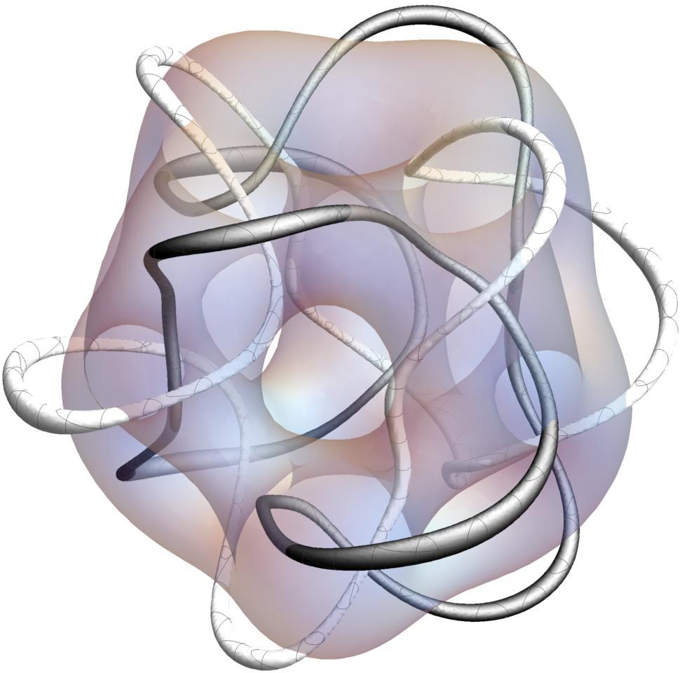
(b) $\boldsymbol{\phi}_{1,2}^{M_{0\frac{3\pi}{2}0}}$

Figure 8: Links for the $B=6$ Skyrmion. (a) Links between the vortex rings (yellow) and the vacuum vortex (magenta) which is degenerate. (b) Nondegenerate links between the vortex and vacuum vortex, which are both closed loops. The gray isosurface is the baryon charge density illustrating the shape of the Skyrmion.

The $B=6$ Skyrmion has $D_{4d}$ dihedral symmetry, which is generated by the rational map Houghton:1997kg

$$R_{6}(z)=\frac{z^{4}+\mathrm{i}a}{z^{2}(\mathrm{i}az^{4}+1)},$$ (50)

with $a\in\mathbb{R}$. This is the first $B$ for which symmetry does not fix the parameters of the rational map. Minimization of $\mathcal{I}$ (eq. (43)) yields $a=0.16$ Houghton:1997kg .

Fig. 8 shows preimages of $\boldsymbol{\phi}_{1,2}$ as well as of a rotation of them by $\beta=\frac{3\pi}{2}$. The vacuum vortex (magenta) in fig. 8(a) is still degenerate as promised, but after a swift $\beta$ rotation, the mapping of the vortex points is regular. After a bit of disentangling, it is clear that the vacuum vortex (white) links the vortex (black) six times in fig. 8(b), corresponding to $q=1$, $p=6$ and $B=Q=pq=6$.

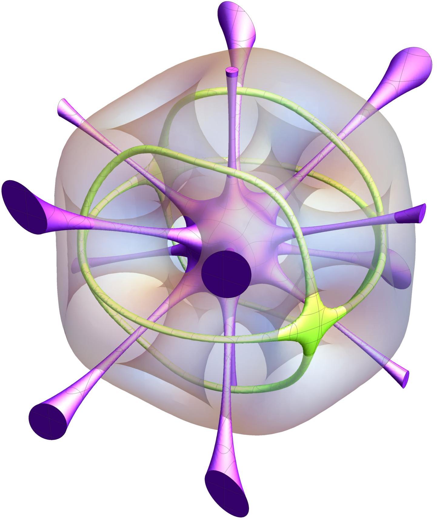
(a) $\boldsymbol{\phi}_{1,2}$

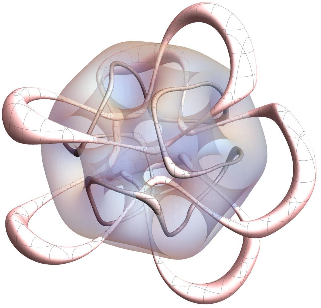
(b) $\boldsymbol{\phi}_{1,2}^{M_{0\frac{\pi}{6}0}}$

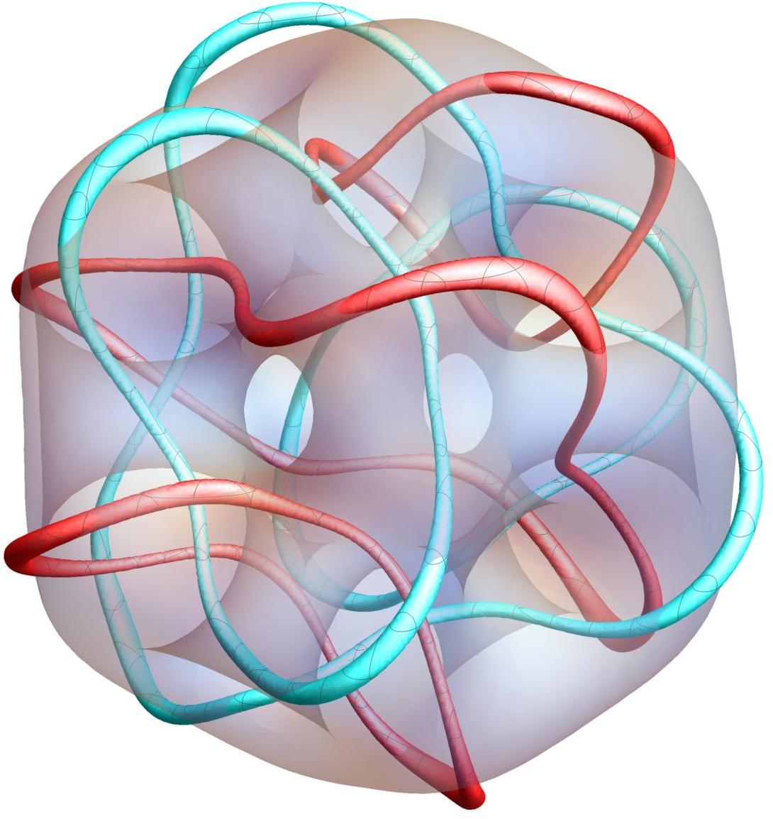
(c) $\boldsymbol{\phi}_{1,2}^{M_{0\frac{\pi}{2}0}}$

Figure 9: Links for the $B=7$ Skyrmion. (a) A link between the vortex ring (yellow) and the vacuum vortex (magenta), which are both degenerate. (b,c) Nondegenerate links between the vortices and vacuum vortices, which are both closed loops. The gray isosurface is the baryon charge density illustrating the shape of the Skyrmion.

The $B=7$ Skyrmion is the most symmetric of them all and possesses icosahedral symmetry, which fixes the rational map as Houghton:1997kg

$$R_{7}(z)=\frac{z^{5}+3}{z^{2}(3z^{5}+1)}.$$ (51)

Fig. 9 shows preimages of $\boldsymbol{\phi}_{1,2}$ as well as of rotations thereof by $\beta=\frac{\pi}{6}$ and by $\beta=\frac{\pi}{2}$. In the canonical frame, both vortices are degenerate. After rotating by $\beta=\frac{\pi}{6}$ the mapping is regular and the vortex (dark red) links three vacuum vortices (ligth red) two, three and two times, respectively, yielding $q=1$, $p=7$, $B=Q=pq=7$. The counting goes slightly different if we continue the rotation of the 2-sphere to $\beta=\frac{\pi}{2}$ where both vortices have turned into 3 rings. If we take the point of view of the red vortices, the winding numbers are $q_{1}=1$, $p_{1}=2$, $q_{2}=1$, $p_{2}=3$, $q_{3}=1$, $p_{3}=2$. Notice, however, that the clusters themselves are linked and therefore the number of vacuum vortices is not 7 but 3.

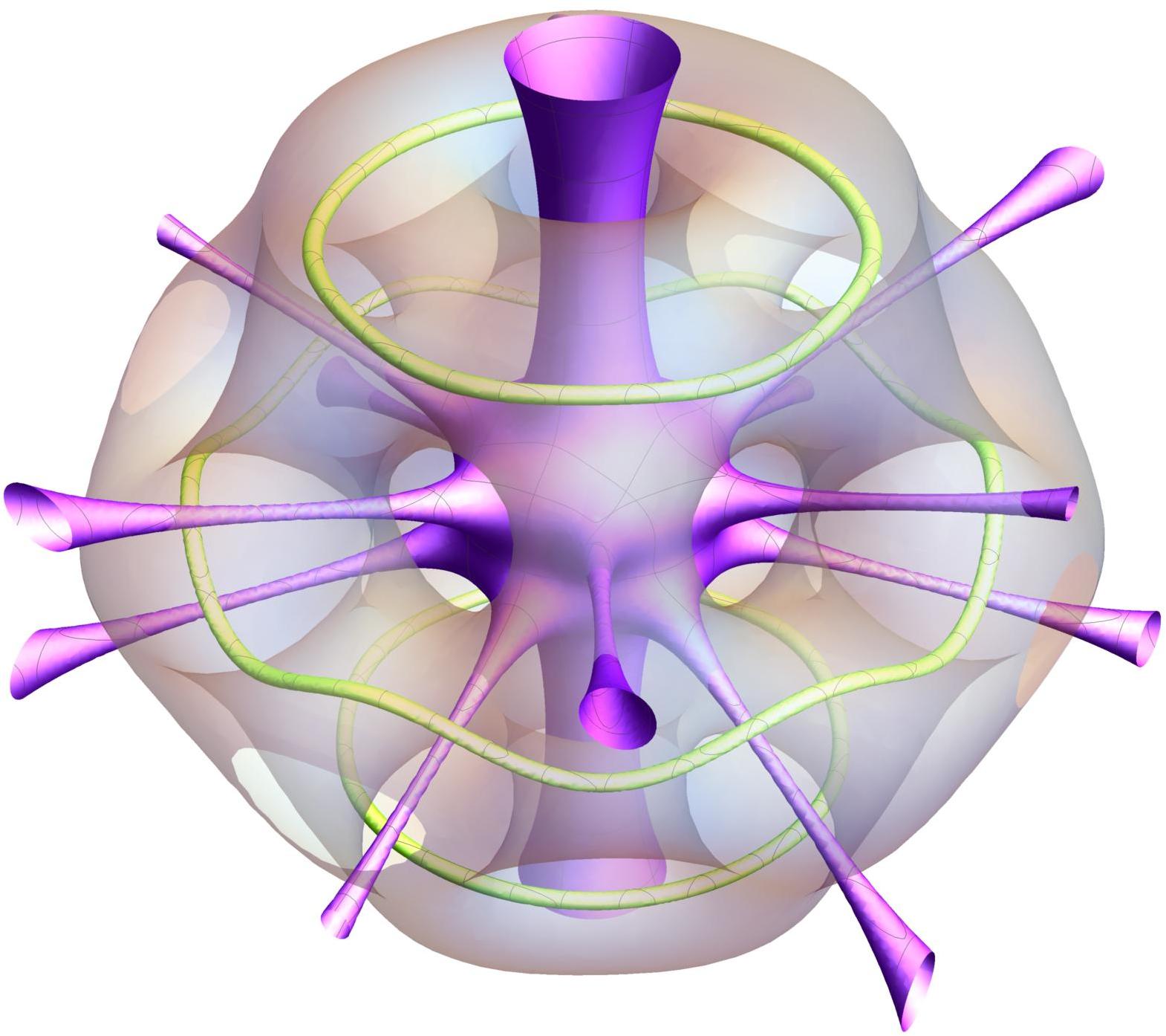
(a) $\boldsymbol{\phi}_{1,2}$

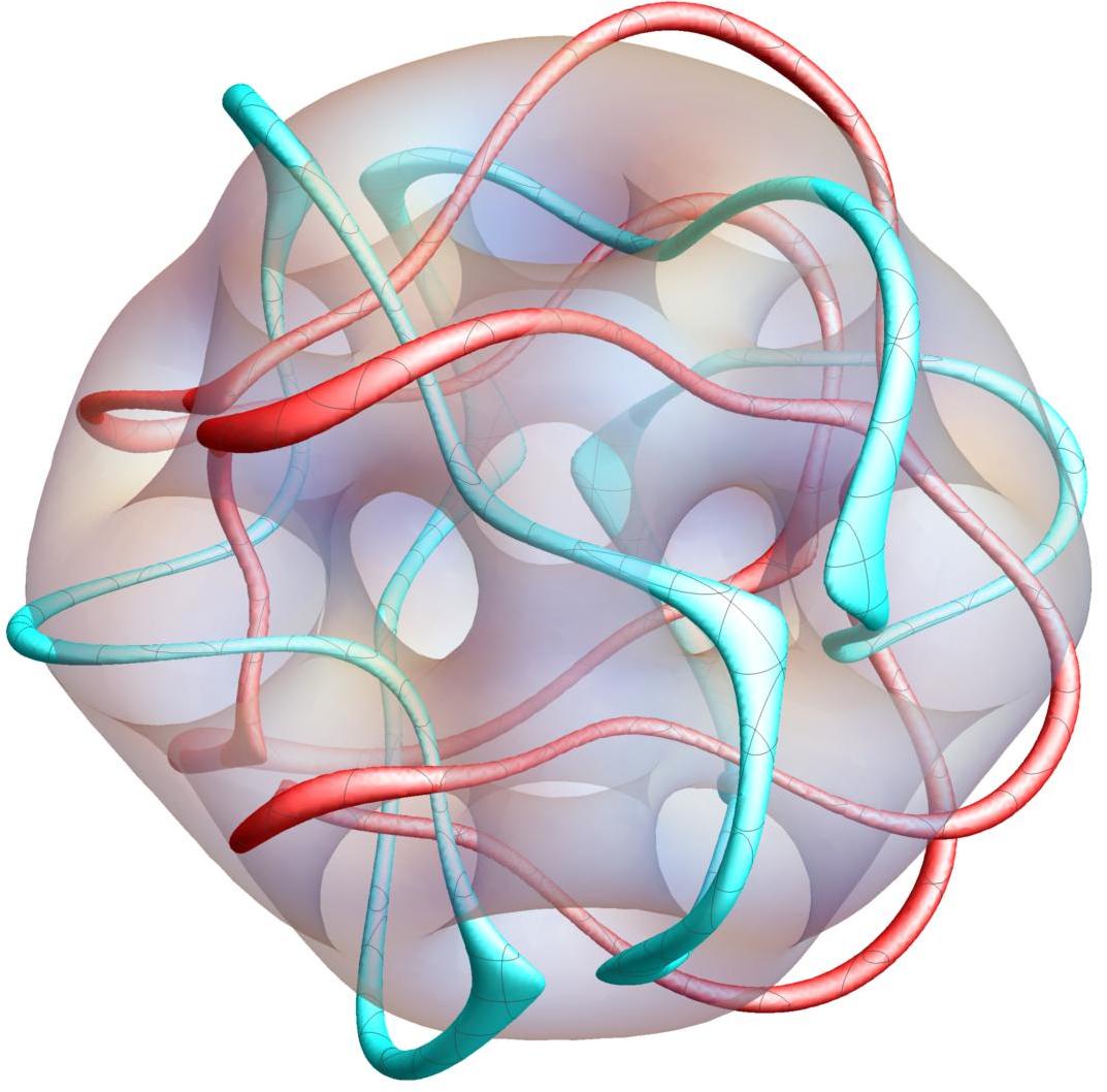
(b) $\boldsymbol{\phi}_{1,2}^{M_{0\frac{\pi}{2}0}}$

(c) $\boldsymbol{\phi}_{1,2}^{M_{0\frac{\pi}{2}\frac{\pi}{4}}}$

Figure 10: Links for the $B=8$ Skyrmion. (a) Links between the vortex rings (yellow) and the vacuum vortex (magenta) which is degenerate. (b,c) Nondegenerate links between the vortices and vacuum vortices, which are both closed loops. The gray isosurface is the baryon charge density illustrating the shape of the Skyrmion.

The last Skyrmion here is the $B=8$ Skyrmion, which has $D_{6d}$ symmetry in the massless theory (41), in contradistinction from the solution of the massive theory which is composed by two cubes Battye:2006na . The rational map for the fullerene-like Skyrmion with $D_{6d}$ symmetry has the corresponding rational map Houghton:1997kg

$$R_{8}(z)=\frac{z^{6}-a}{z^{2}(az^{6}+1)},$$ (52)

with $a\in\mathbb{R}$. The minimization of $\mathcal{I}$ of eq. (43) yields $a=0.14$ Houghton:1997kg .

Fig. 10 shows preimages of $\boldsymbol{\phi}_{1,2}$ as well as of rotations thereof by $\beta=\frac{\pi}{2}$ and by $\gamma=\frac{\pi}{4}$. As expected by now, the vacuum vortex in fig. 10(a) is degenerate. In fig. 10(b) the vacuum vortex (cyan) and the vortex (red) are linked eight times and the counting is simply $q=1$, $p=8$, and thus $B=Q=pq=8$. Rotating by $\pi/4$ around the equator of the 2-sphere, yields different preimages. Now there are three vortices (yellow), see fig. 10(c), that link the vacuum vortex (blue) and they link the vacuum vortex two, four and two times, respectively. The counting now goes like $q_{1}=1$, $p_{1}=2$, $q_{2}=1$, $p_{2}=4$, $q_{3}=1$, $p_{3}=2$ and thus we have $B=Q=\sum_{\ell=1}^{3}p_{\ell}q_{\ell}=8$ again, as promised.

4 Discussion and outlook

In this paper, we have proved theorem 1 which states that the degree of a Skyrme field is the same as the linking number of two preimages of two distinct regular points on the 2-sphere of said field under the Hopf map. We further conjecture that the 2 linked lines may be interpreted as vortices in the original O(4) field. Note that such an interpretation is impossible in the Faddeev-Skyrme model which is based on O(3) fields in $\mathbb{R}^{3}$, although they do possess Hopf charge and knots.

We illustrated the conjecture and hence the theorem with two examples: a toroidal vortex, which is simply an axially symmetric Skyrmion with topological degree $P$ (energetically stabilized by a certain potential, see ref. Gudnason:2016yix ); and with the eight first rational map Skyrmions of ref. Houghton:1997kg .

The toroidal vortex or the $P$-wound axially symmetric Skyrmion is in fact the motivation for conjecture 1 and naturally it works well. The rational map Skyrmions, on the other hand, are a nontrivial check on the conjecture and so far it has passed the checks.

One should note that all the preimages that we studied in this paper are themselves unknots, viz. they are topologically equivalent to circles. So we have only checked the conjecture 1 with various numbers of linked unknots. It is possible that the conjecture needs refinement in more complicated situations where the preimage itself become links or a knot or even linked knots, which then by the nature of the game will be linked with the other preimage. Although $B=Q$ holds by theorem 1, the conjecture may receive corrections of the form, schematically

$$B=Q=\sum_{\rm unknots}pq+\sum_{\rm links}F_{\rm links}(p,q)+\sum_{\rm knots}F_{\rm knots}(p,q)+\sum_{\rm linked\ knots}F_{\rm linked\ knots}(p,q),$$ (53)

where we have suppressed cluster indices. We leave this for future studies.

Lord Kelvin imagined that atoms are described by knots of vortices Thomson:1869 . With theorem 1 we can say that nuclei are not knots, but contain links of vortices via a certain projection.

Acknowledgments

We would like to thank Michikazu Kobayashi for collaboration at the early stage of this work and we thank Chris Halcrow, Steffen Krusch, Martin Speight and Paul Sutcliffe for discussions and comments. S. B. G. thanks the Outstanding Talent Program of Henan University for partial support. The work of S. B. G. is supported by the National Natural Science Foundation of China (Grant No. 11675223). M. N. is supported by the Ministry of Education, Culture, Sports, Science (MEXT)-Supported Program for the Strategic Research Foundation at Private Universities “Topological Science” (Grant No. S1511006) and by a Grant-in-Aid for Scientific Research on Innovative Areas “Topological Materials Science” (KAKENHI Grant No. 15H05855) from MEXT, Japan. M. N. is also supported in part by the Japan Society for the Promotion of Science (JSPS) Grant-in-Aid for Scientific Research (KAKENHI Grant No. 16H03984 and No. 18H01217).

References

- (1) N. Manton and P. Sutcliffe, “Topological Solitons,” Cambridge University Press (2004).
- (2) R. S. Ward, “Hopf solitons from instanton holonomy,” Nonlinearity 14, 1543 (2001) [hep-th/0108082].
- (3) R. A. Battye and P. M. Sutcliffe, “Knots as stable soliton solutions in a three-dimensional classical field theory.,” Phys. Rev. Lett. 81, 4798 (1998) [hep-th/9808129].
- (4) R. A. Battye and P. Sutcliffe, “Solitons, links and knots,” Proc. Roy. Soc. Lond. A 455, 4305 (1999) [hep-th/9811077].
- (5) L. D. Faddeev and A. J. Niemi, “Knots and particles,” Nature 387, 58 (1997) [hep-th/9610193].
- (6) U. G. Meissner, “Toroidal Solitons With Unit Hopf Charge,” Phys. Lett. 154B, 190 (1985).
- (7) R. S. Ward, “Skyrmions and Faddeev-Hopf solitons,” Phys. Rev. D 70, 061701 (2004) [hep-th/0407245].
- (8) J. Gladikowski and M. Hellmund, “Static solitons with nonzero Hopf number,” Phys. Rev. D 56, 5194 (1997) [hep-th/9609035].
- (9) S. B. Gudnason and M. Nitta, “Skyrmions confined as beads on a vortex ring,” Phys. Rev. D 94, no. 2, 025008 (2016) [arXiv:1606.00336 [hep-th]].
- (10) S. B. Gudnason and M. Nitta, “Effective field theories on solitons of generic shapes,” Phys. Lett. B 747, 173 (2015) [arXiv:1407.2822 [hep-th]].
- (11) S. B. Gudnason and M. Nitta, “Incarnations of Skyrmions,” Phys. Rev. D 90, no. 8, 085007 (2014) [arXiv:1407.7210 [hep-th]].
- (12) S. B. Gudnason and M. Nitta, “Baryonic torii: Toroidal baryons in a generalized Skyrme model,” Phys. Rev. D 91, no. 4, 045027 (2015) [arXiv:1410.8407 [hep-th]].
- (13) S. B. Gudnason and M. Nitta, “Baryonic handles: Skyrmions as open vortex strings on a domain wall,” Phys. Rev. D 98, no. 12, 125002 (2018) [arXiv:1809.01025 [hep-th]].
- (14) K. Kasamatsu, M. Tsubota, and M. Ueda, “Vortices in multicomponent Bose–Einstein condensates,” Int. J. Mod. Phys. B19, 1835 (2005) [cond-mat/0505546].
- (15) J. Ruostekoski and J. R. Anglin, “Creating vortex rings and three-dimensional skyrmions in Bose-Einstein condensates,” Phys. Rev. Lett. 86, 3934 (2001) [cond-mat/0103310].
- (16) R. A. Battye, N. R. Cooper and P. M. Sutcliffe, “Stable skyrmions in two component Bose-Einstein condensates,” Phys. Rev. Lett. 88, 080401 (2002) [cond-mat/0109448].
- (17) M. Nitta, K. Kasamatsu, M. Tsubota and H. Takeuchi, “Creating vortons and three-dimensional skyrmions from domain wall annihilation with stretched vortices in Bose-Einstein condensates,” Phys. Rev. A 85, 053639 (2012) [arXiv:1203.4896 [cond-mat.quant-gas]].
- (18) C. J. Houghton, N. S. Manton and P. M. Sutcliffe, “Rational maps, monopoles and Skyrmions,” Nucl. Phys. B 510, 507 (1998) [hep-th/9705151].
- (19) R. Battye, N. S. Manton and P. Sutcliffe, “Skyrmions and the alpha-particle model of nuclei,” Proc. Roy. Soc. Lond. A 463, 261 (2007) [hep-th/0605284].
- (20) W. H. Thomson, “On Vortex Motion,” Trans. R. Soc. Edin. 25, 217 (1868).