Three planets transiting the evolved star EPIC 249893012:
a hot 8.8-M_⊕ super-Earth and two warm 14.7 and 10.2-M_⊕ sub-Neptunes,,

We report the discovery of a new planetary system with three transiting planets, one super-Earth and two sub-Neptunes, that orbit EPIC 249893012, a G8 IV-V evolved star ($M_{\star}$ = 1.05 $\pm$ 0.05 $M_{\odot}$, $R_{\star}$ = 1.71 $\pm$ 0.04 $R_{\odot}$, $T_{\mathrm{eff}}$ =5430 $\pm$ 85 K). The star is just leaving the main sequence. We combined K2 photometry with IRCS adaptive-optics imaging and HARPS, HARPS-N, and CARMENES high-precision radial velocity measurements to confirm the planetary system, determine the stellar parameters, and measure radii, masses, and densities of the three planets. With an orbital period of $3.5949^{+0.0007}_{-0.0007}$ days, a mass of $8.75^{+1.09}_{-1.08}\ M_{\oplus}$ , and a radius of $1.95^{+0.09}_{-0.08}\ R_{\oplus}$, the inner planet b is compatible with nickel-iron core and a silicate mantle ($\rho_{b}=6.39^{+1.19}_{-1.04}$ g cm^-3). Planets c and d with orbital periods of $15.624^{+0.001}_{-0.001}$ and $35.747^{+0.005}_{-0.005}$ days, respectively, have masses and radii of $14.67^{+1,84}_{-1.89}\ M_{\oplus}$ and $3.67^{+0.17}_{-0.14}\ R_{\oplus}$ and $10.18^{+2.46}_{-2.42}\ M_{\oplus}$ and $3.94^{+0.13}_{-0.12}\ R_{\oplus}$, respectively, yielding a mean density of $1.62^{+0.30}_{-0.29}$ and $0.91^{+0.25}_{-0.23}$ g cm^-3, respectively. The radius of planet b lies in the transition region between rocky and gaseous planets, but its density is consistent with a rocky composition. Its semimajor axis and the corresponding photoevaporation levels to which the planet has been exposed might explain its measured density today. In contrast, the densities and semimajor axes of planets c and d suggest a very thick atmosphere. The singularity of this system, which orbits a slightly evolved star that is just leaving the main sequence, makes it a good candidate for a deeper study from a dynamical point of view.

1 Introduction

With the advent of space-based transit-search missions, the detection and characterization of exoplanets have undergone a fast-paced revolution. First CoRoT (Auvergne et al., 2009) and then Kepler (Borucki et al., 2010) marked a major leap forward in understanding the diversity of planets in our Galaxy. With the failure of its second reaction wheel, Kepler embarked on an extended mission, named K2 (Howell et al., 2014), which surveyed different stellar fields located along the ecliptic. Their high-precision photometry has allowed the Kepler and K2 missions to dramatically extended the parameter space of exoplanets, bringing the transit detection threshold down to the Earth-sized regime. The Transiting Exoplanet Survey Satellite (TESS; Ricker et al., 2015) is currently extending this search to cover almost the entire sky; it mainly focuses on bright stars (V $<$ 11).

Although super-Earths ($R_{\mathrm{p}}$ $\simeq$ $1-2$ $R_{\oplus}$, $M_{\mathrm{p}}$ $\simeq$ $1-10$ $M_{\oplus}$) and Neptune-sized planets ($R_{\mathrm{p}}$ $\simeq$ $2-4$ $\ R_{\oplus}$, $M_{\mathrm{p}}$ $\simeq$ $10-40$ $\,M_{\oplus}$) are ubiquitous in our Galaxy (see, e.g., Marcy et al., 2014; Silburt et al., 2015; Hsu et al., 2019), we still have much to learn about the formation and evolution processes of small planets. Observations have led to the discovery of peculiar patterns in the parameter space of small exoplanets (Winn, 2018). The radius–period diagram shows a dearth of short-period Neptune-sized planets, the so-called Neptunian desert (Mazeh et al., 2016; Owen & Lai, 2018). Small planets tend to prefer radii of either $\sim$1.3 $R_{\oplus}$ or $\sim$2.6 $R_{\oplus}$, with a dearth of planets at $\sim$1.8 $R_{\oplus}$, the so-called radius gap (Fulton et al., 2017; Fulton & Petigura, 2018). Atmospheric erosion by high-energy stellar radiation (also known as photoevaporation) is believed to play a major role in shaping both the Neptunian desert and the bimodal distribution of planetary radii. Moreover, Armstrong et al. (2019) found a gap in the mass distribution of planets with a mass lower than $\sim$20 $M_{\oplus}$ and periods shorter than 20 days, so far without any apparent physical explanation.

Understanding the formation and evolution of small planets requires precise and accurate measurements of their masses and radii. The KESPRINT consortium aims at confirming and characterizing planetary systems from the K2 mission (see, e.g., Grziwa et al., 2016; Gandolfi et al., 2017; Prieto-Arranz et al., 2018; Luque et al., 2019; Palle et al., 2019), and more recently, from the TESS mission (Esposito et al., 2019; Gandolfi et al., 2018, 2019).

This paper is organized as follows: in Sect. 2 we describe the K2 photometry together with the detection of the three transiting planets and a preliminary fit of their transit light curves. In Sect. 3 we describe our follow-up observations. The stellar fundamental parameters are provided in Sect. 4. In Sect. 5 we present the frequency analysis of the radial velocity measurements; the joint modeling is described in Sect. 6. Discussion and conclusions are given in Sect. 7.

2 K2 photometry and detection

EPIC 249893012 was observed during K2 Campaign 15 of K2 as part of the K2 guest observer (GO) programs GO-15052 (PI: Stello D.) and GO-15021 (PI: Howard, A. W.). Campaign 15 lasted 88 days, from 23 August 2017 to 20 November 2017, observing a patch of sky toward the constellations of Libra and Scorpius. During Campaign 15, the Sun emitted 27 M-class and four X-class flares and released several powerful coronal mass ejections (CMEs). This affected the measured dark current levels for all K2 channels. Peak dark current emissions occurred around BJD 2458003.23, 2458007.85, and 2458009.00 (3170.23, 3174.85 and 3176.00, respectively, for the time reference value, BJD - 2454833, given in Fig. 2).

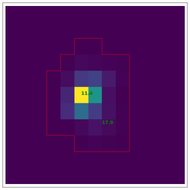
Figure 1: Customized K2 image of EPIC 249893012. North is to the left and east at the bottom. The field of view is 43.78$\times$51.74 arcsec (3.98 arcsec per pixel). The red line marks the customized aperture for light-curve extraction, with a threshold of 1.7$\sigma$ above the background. Green annotations are the Kepler magnitude (retrieved from the RA and DEC from MAST) of EPIC 249893012, and the source of contamination is identified in Fig.5.

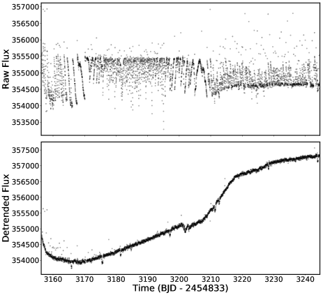
Figure 2: K2 light curves of EPIC 249893012. The upper panel shows the raw light curve as extracted from the pixel data file in units of electrons per cadence. The lower panel shows the detrended light curve as obtained using our Everest-based pipeline. No stellar variability is detectable but the transit signals are clearly visible.

We built the light curve of EPIC 249893012 from the target pixel file downloaded from the Mikulski Archive for Space Telescopes (MAST). The pipeline used in this paper is based on the pixel level decorrelation (PLD) method that was initially developed by Deming et al. (2015) to correct the intra-pixel effects for Warm Spitzer data, and which was implemented in a modified and updated version of the Everest pipeline (Luger et al., 2018). Our pipeline customizes different apertures for every single target by selecting the photocenter of the star and the nearest pixels, with a threshold of 1.7$\sigma$ above the previously calculated background (Fig. 1). After the aperture pixels were chosen, our pipeline extracted the raw light curve and removed all time cadences that were flagged as bad-quality data. The pipeline applies PLD to the data up to third order to perform robust flat-fielding corrections, which avoids us having to solve for correlations on stellar positions. It also uses a second step of Gaussian processes (GP), which separates astrophysical and instrumental variability, to compute the covariance matrix as described in Luger et al. (2018). The raw and the final detrended light curves are plotted in Fig. 2. Our pipeline, which is based on EVEREST, tends to introduce long-term modulation, masking low-frequency signals such as the stellar variability that is uncovered with the frequency analysis of the radial velocity data in section 5.

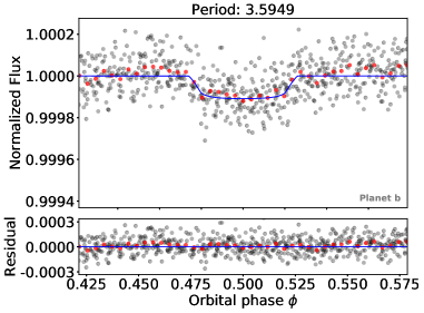
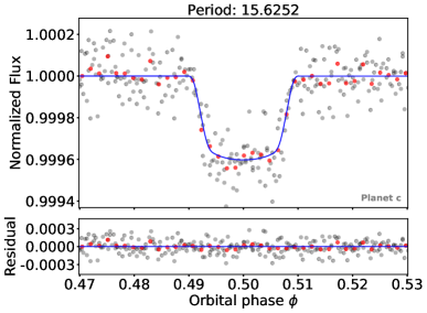
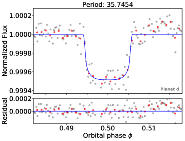
Figure 3: Phase-folded transit light curves of EPIC 249893012 b, c, and d (upper, middle, and lower panel, respectively). The black points mark the detrended K2 data. The red points mark the bins of 15 (top panel), 6 (middle panel), and 4 data points (bottom panel). The blue solid line represents the best-fit transit model for each planet. Residuals are shown in the lower panels of each transit light curve.

We used a robust locally weighted regression method (Cleveland, 1979), with a fraction parameter of 0.04, to flatten the light curve. We also used this method with a lower fraction rate to interactively detect and remove outliers above 3$\sigma$ until no points were detected. We removed the data observed from the first three and a half days of the campaign, from BJD 2457989.44 to 2457993.0 (3156,44 to 3160.00 for the BJD - 2454833 time reference in Fig. 2), because of a sharp trend at the beginning of the observation that is probably related to a thermal anomaly. We finally flattened the original light curve by dividing it by the model.

We searched the flattened light curve for transits using the box-fitting least squares (BLS) algorithm (Kovács et al., 2002). When a planetary signal was detected in the power spectrum, we fit a transit model using the python package batman (Kreidberg, 2015). We divided the transit model by the flattened light curve and again applied the BLS algorithm to find the next planetary signal, until no significant peak was found in the power spectrum.

We found three planetary signals in the EPIC 249893012 light curve, with periods of 3.59, 15.63, and 35.75 days and depths of 108.7, 402.3 and 484.3 ppm. The period ratios are 1:4.34:9.94, out of resonance, except for signals b and d with a ratio close to 1:10. Figure 3 shows the phase-folded light curve for each transit signal and the best-fit model.

3 Ground-based follow-up observations

3.1 High-resolution imaging

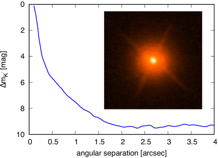
Figure 4: 5 $\sigma$ contrast curve against angular separation from EPIC 249893012, based on the IRCS AO imaging. The inset exhibits EPIC 249893012 $4^{\prime\prime}\times 4^{\prime\prime}$ image.

On 14 July 2019, we performed adaptive-optics (AO) imaging for EPIC 249893012 with the InfraRed Camera and Spectrograph (IRCS: Kobayashi et al., 2000) on the Subaru 8.2m telescope to search for faint nearby sources that might contaminate the K2 photometry. Adopting the target star itself as a natural guide for AO, we imaged the target in the $K^{\prime}$ band with a five-point dithering. We obtained both short-exposure (unsaturated; $0.5s\times 3$ coaddition for each dithering position) and long-exposure (mildly saturated; $2.0s\times 3$ coaddition for each) frames of the target for absolute flux calibration and for inspecting nearby faint sources, respectively. We reduced the IRCS data following Hirano et al. (2016), and obtained the median-combined images for unsaturated and saturated frames, respectively. Based on the unsaturated image, we estimated the target full width at half-maximum (FWHM) to be $0\aas@@fstack{\prime\prime}115$. In order to estimate the detection limit of nearby faint companions around EPIC 249893012, we computed the 5 $\sigma$ contrast as a function of angular separation based on the flux scatter in each small annulus from the saturated target. Figure 4 plots the 5 $\sigma$ contrast along with the $4^{\prime\prime}\times 4^{\prime\prime}$ target image in the inset. Our AO imaging achieved approximately $\Delta K^{\prime}=8$ mag at $1^{\prime\prime}$ from EPIC 249893012.

Visual inspection of the saturated image suggests no nearby companion within $5^{\prime\prime}$ from EPIC 249893012, but it exhibits a faint source separated by $8\aas@@fstack{\prime\prime}3$ in the southeast (Fig. 5), that is, inside the aperture for light-curve extraction on the K2 image (see Fig. 1). Checking the Gaia DR2 catalog, we found that this faint source is the Gaia DR2 6259260177825579136 star with $G=17.9$ mag (Gaia G magnitude defined in Evans et al., 2018); further information of this source is provided in Table 1. The transit signal with depth of 100 ppm on EPIC 249893012 ($K_{p}=11.364$ mag) may be mimicked by an equal-mass eclipsing binary that is 9.29 magnitude fainter, that is, with a Kepler magnitude of 20.65. Taking into account the close similarity between the Gaia and Kepler bandpasses, we therefore cannot exclude Gaia DR2 6259260177825579136 as a source of a false positive for one of the three transit signals (see Sect. 4.3).

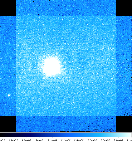
Figure 5: Adaptive-optics image of EPIC 249893012 obtained with the Subaru/IRCS instrument. North is up and east is to the left. Field of view of is 21″ in both directions (pixel scale of $0\aas@@fstack{\prime\prime}02$/pix). Because this image was created after median-combining the aligned frames, background levels as well as flux scatters in the corners are different from those of the central part of the detector.

3.2 High-resolution spectroscopy

We collected 74 high-resolution (R$\approx$115 000) spectra of EPIC 249893012 using the High Accuracy Radial velocity Planet Searcher (HARPS) spectrograph (Mayor et al., 2003) mounted at the ESO-3.6m telescope of the La Silla observatory (Chile). The observations were carried out between April 2018 and August 2019 as part of our radial velocity (RV) follow-up of K2 and TESS planets conducted with the HARPS spectrograph (observing programs 0101.C-0829 and 1102.C-0923; PI: Gandolfi) and under program 60.A-9700 (technical time). We reduced the data using the HARPS Data Reduction Software (DRS) and extracted the Doppler measurements by cross-correlating the Echelle spectra with a G2 numerical mask (Baranne et al., 1996; Pepe et al., 2002; Lovis & Pepe, 2007). The DRS also provides the user with the FWHM and the bisector inverse slope (BIS) of the cross-correlation function (CCF), as well as with the Ca ii H & K lines activity indicator log R${}^{\prime}_{\mathrm{HK}}$.

Between April 2018 and March 2019, we also secured 11 high-resolution (R$\approx$115 000) spectra with the HARPS-N spectrograph (Cosentino et al., 2012) mounted at the 3.58m Telescopio Nazionale Galileo at Roque de Los Muchachos observatory (La Palma, Spain), as part of the observing programs CAT18A_130, CAT18B_93 (PI: Nowak), and A37TAC_37 (PI: Gandolfi). The data reduction, as well as the extraction of the RV measurements and activity- and line-profile indicators follows the same procedure as for the HARPS spectra.

Between 6 May 2018 and 21 June 2018, we also collected 25 spectra of EPIC 249893012 with the Calar Alto high-Resolution search for M dwarfs with Exoearths with Near-infrared and optical Échelle Spectrographs (CARMENES) instrument (Quirrenbach et al., 2014, 2018), installed at the 3.5m telescope of Calar Alto Observatory in Spain (observing program S18-3.5-021 – PI: Pallé.). The instrument consists of a visual (VIS, $0.52\text{\,}\mathrm{-}$$0.96\text{\,}\mathrm{\SIUnitSymbolMicro m}$) and a near-infrared (NIR, $0.96\text{\,}\mathrm{-}$$1.71\text{\,}\mathrm{\SIUnitSymbolMicro m}$) channel yielding spectra at a resolution of $R\,\approx\,94\,600$ and $R\approx 80\,400$, respectively. Like Luque et al. (2019), we only used the VIS observations to extract the RV measurements because the spectral type of EPIC 249893012 is solar like. We computed the CCF using a weighted mask constructed from the coadded CARMENES VIS spectra of EPIC 249893012 and determined the RV, FWHM, and the BIS measurements by fitting a Gaussian function to the final CCF following the method described in Reiners et al. (2018).

Tables 4, 5, and 6 list the HARPS, HARPS-N, and CARMENES Doppler measurements and their uncertainties, along with the BIS and FWHM of the CCF, the exposure time, the signal-to-noise ratio (S/N) per pixel at 5500 Å for HARPS and HARPS-N, and at 5340 Å for CARMENES, and for HARPS and HARPS-N alone, the Ca ii H & K activity index log R${}^{\prime}_{\mathrm{HK}}$.

Table 1: Relative properties of the nearby star to EPIC 249893012 detected with the Subaru/IRCS.

Parameter	close-in star
Separation (″)	$8.30\pm 0.03$
Position Angle (deg)	$124.12\pm 0.10$
$\Delta m_{K^{\prime}}$ (mag)	$6.697\pm 0.023$
$\Delta F_{K^{\prime}}$ relative flux	$(2.095\pm 0.044)\times 10^{-3}$

4 Stellar properties

Table 2: Equatorial coordinates, main identifiers, optical and infrared magnitudes, proper motion, parallax, distance, spectroscopic parameters, interstellar extinction and fundamental parameters of EPIC 249893012.

Parameter	Value	Source
Equatorial Coordinates and Main Identifiers
RAJ2000.0 (hh:mm:ss)	15:12:59.57	Gaiaa
DECJ2000.0 (dd:mm:ss)	$-$16:43:28.73	Gaiaa
Gaia ID	6259263137059042048	Gaiaa
2MASS ID	J15125956-1643282	2MASSb
TYC ID	6170-95-1	TYCHO2c
Optical and Near-Infrared Magnitudes
$K_{p}$ (mag)	11.364	K2d
$B_{J}$ (mag)	12.335 $\pm$ 0.240	K2d
$V_{J}$ (mag)	11.428 $\pm$ 0.121	K2d
$G$ (mag)	11.4019 $\pm$ 0.0005	Gaiaa
$g$ (mag)	11.911 $\pm$ 0.010	K2d
$r$ (mag)	11.370 $\pm$ 0.020	K2d
$i$ (mag)	11.130 $\pm$ 0.030	K2d
$J$ (mag)	10.216 $\pm$ 0.026	K2d
$H$ (mag)	9.800 $\pm$ 0.023	K2d
$K$ (mag)	9.714 $\pm$ 0.023	K2d
Space Motion and Distance
PMRA (mas  yr-1)	13.55 $\pm$ 0.07	Gaiaa
PMDEC (mas  yr-1)	$-$34.29 $\pm$ 0.06	Gaiaa
Parallax (mas)	3.08 $\pm$ 0.04	Gaiaa
Distance (pc)	324.7 $\pm$ 4.2	Gaiaa
Spectroscopic Parameters and Interstellar Extinction
Spectral type	G8 IV/V	This work
$T_{\rm eff}$ (K)	5430 $\pm$ 85	This work
log g⋆ (cgs)	3.99 $\pm$ 0.03	This work
[Fe/H] (dex)	0.20 $\pm$ 0.05	This work
[Mg/H] (dex)	0.28 $\pm$ 0.05	This work
[Na/H] (dex)	0.25 $\pm$ 0.05	This work
[Ca/H] (dex)	0.18 $\pm$ 0.05	This work
$V_{\rm mac}$ (km s-1)	3.5 $\pm$ 0.4	This work
$V_{\rm mic}$ (km s-1)	0.9 $\pm$ 0.1	This work
$V\sin i_{\star}$ (km s-1)	2.1 $\pm$ 0.5	This work
$A_{\mathrm{V}}$ (mag)	0.19 $\pm$ 0.02	This work
Stellar Fundamental Parameters
$M_{\star}$($M_{\odot}$)	1.05 $\pm$ 0.05	This work
$R_{\star}$($R_{\odot}$)	1.71 $\pm$ 0.04	This work
	1.81${}^{+0.11}_{-0.27}$	Gaiaa
$L_{\star}$ ($L_{\odot}$)	2.26${}^{+0.04}_{-0.05}$	Gaiaa
$\rho_{\star}$ (g cm-3)	0.298${}^{+0.026}_{-0.023}$	This work
Age (Gyr)	9.0${}^{+0.5}_{-0.6}$	This work

• Gaia DR2 (Gaia Collaboration et al., 2018).

• 2MASS Catalog (Skrutskie et al., 2006).

• TYCHO2 Catalog (Høg et al., 2000).

• ExoFOP.

4.1 Photospheric parameters

We extracted the spectroscopic parameters of the host star from the co-added HARPS spectrum – which has a S/N ratio per pixel of S/N=270 at 5500 Å – using two publicly available packages, as described in the following paragraphs.

We first used the package Spectroscopy Made Easy (SME), version 5.22, (Valenti & Piskunov, 1996; Valenti & Fischer, 2005; Piskunov & Valenti, 2017). SME calculates the equation of state, the line and continuum opacities, and the radiative transfer over the stellar surface with the help of a library of stellar models. A chi-square minimization procedure is then used to extract spectroscopy parameters, that is, the effective temperature $T_{\rm eff}$, the surface gravity log g_⋆, the metal content, the micro $V_{\rm mic}$ and macro $V_{\rm mac}$ turbulent velocities, and the projected-rotational velocity $V\sin i_{\star}$, as described in Fridlund et al. (2017) and Persson et al. (2018, 2019). When any of the parameters listed above an be determined with another method and it can be held fixed during the iterative procedure, this improves the determination of the remaining parameters. The turbulent velocities can typically be obtained as soon as the $T_{\rm eff}$ is derived and/or can be inferred from empirical equations such as those of Bruntt et al. (2010) and Doyle et al. (2014). In the case of EPIC 249893012, we iteratively determined $T_{\rm eff}$  by fitting the wings of the Balmer lines and then proceeded to obtain the other parameters. We selected the grid of ATLAS12 models (Kurucz, 2013) as the basis for our analysis. After obtaining the relevant abundances of metals, log g_⋆ was obtained by fitting the spectral lines of Mg I and Ca I and checking by finally analyzing the Na i doublet. The values for each parameter can be found in the Table 2. The result indicates a somewhat evolved solar-type star with a log g_⋆ of 3.8-3.9. Atomic and molecular parameters needed for the analysis were downloaded from the VALD database (Ryabchikova & Pakhomov, 2015).

We also used the package specmatch-emp (Yee et al., 2017), which uses a library of $\sim$400 high-resolution template spectra of well-characterized FGKM stars obtained with the HIRES spectrograph on the Keck telescope. We used a custom algorithm to put our HARPS spectrum into the same format as the HIRES spectra (Hirano et al., 2018), which was then compared to the spectra within the library to find the best match. specmatch-emp provides the effective temperature $T_{\rm eff}$ and iron content [Fe/H], along with the stellar radius, $R_{\star}$. We found values for $T_{\rm eff}$ and [Fe/H] within 1 $\sigma$ of the SME-derived values, as well as a stellar radius of $R_{\star}$ = 1.4 $\pm$ 0.2 R_⊙, which is consistent with the radius derived in Sect. 4.2. The spectroscopic parameters of EPIC 249893012 imply a spectral type and luminosity class of G8 IV/V (Cox & Pilachowski, 2000; Gray, 2008).

4.2 Stellar mass, radius, and age

Our data enable the measurement of the planetary fundamental parameters, most notably, the planetary radius, mass, and mean density. However, the stellar parameters are dependent on the properties of the host star. In order to extract the planetary properties and evaluate the evolutionary status of the planet, we need to derive the physical stellar parameters such as $M_{\star}$, $R_{\star}$, and age (assumed to be the same as that of the planet) using the spectral data.

We began by applying the spectroscopic parameters of Sect. 4.1 to the Torres et al. (2010) empirical relation and derived preliminary estimates of the a stellar mass (1.3 $\pm$ 0.1 M_⊙) and radius (2.3 $\pm$ 0.5 R_⊙). In order to improve the precision, we used the Gaia parallax (Gaia Collaboration et al., 2018) along with the magnitudes listed in Table 2 and estimated the interstellar extinction along the line of sight to the star in two ways. The first method fits the spectral energy distribution (SED) using low-resolution synthetic spectra, as described in Gandolfi et al. (2008), and gives an extinction of $A_{\mathrm{V}}$ = 0.25 $\pm$ 0.08. The second method uses a 3D galactic dust map (Green et al., 2018) to provide the extinction as $A_{\mathrm{V}}$ = 0.19 $\pm$ 0.02. The two methods are consistent within the uncertainties. We used the bolometric correction $BC_{\mathrm{V}}$ derived using the Torres (2010) corrections to the empirical equation of Flower (1996) to derive the radius of the star as 1.67 $\pm$ 0.09 R_⊙. We confirmed this value through the calculation of model tracks using the Bayesian PARAM 1.3 webtool (da Silva et al., 2006). Here we used the spectroscopic parameters, the dereddened Johnson visual magnitude $V_{J}$, and Gaia parallax. PARAM 1.3 gives a stellar mass of 1.1 $\pm$ 0.02 M_⊙ with a radius consistent with the result derived above from the parallax and (dereddened) magnitude. The age is found to be about 7-8 Gyr.

Finally, we used the BAyesian STellar Algorithm (BASTA, Silva Aguirre et al., 2015) with a grid of MESA (Modules for Experiments in Stellar Astrophysics, Paxton et al., 2011) stellar models to perform a joint fit to the SED ($B_{J},V_{J},J,H,K,G$) and spectroscopic parameters $T_{\rm eff}$, $\log g$, [Fe/H]. We adopted the extinction by Green et al. (2018) and corrected the parallax for the offset found in Stassun & Torres (2018) while quadratically adding $0.1$ mas to the uncertainty to account for systematics in the Gaia DR2 data (Luri et al., 2018). We likewise corrected the Gaia $G$-band magnitude following Casagrande & VandenBerg (2018) and adopted an uncertainty of 0.01 mag. We found consistent values of $M_{\star}$ = 1.05 $\pm$ 0.05 M_⊙, $R_{\star}$ = 1.71 $\pm$ 0.04 R_⊙and an age of 9.0${}^{+0.5}_{-0.6}$ Gyr. We adopted these parameters for the analysis presented in the following sections.

The empirical and evolutionary model-dependent derivation of the stellar parameters, coupled with our spectroscopic parameters and Gaia parallax, confirm that EPIC 249893012 is a G-type star slightly more massive than the Sun in its first stages of evolution off the main sequence. Thus, it has a slightly lower $T_{\rm eff}$ than the Sun with a somewhat larger radius, as inferred by its significantly lower value of log g_⋆.

4.3 Faint AO companion

The faint star detected in the Subaru/IRCS AO image and identified as the Gaia DR2 6259260177825579136 star (see Section 3.1) cannot be excluded as a possible source of one of the transit signals detected in the K2 light curve of EPIC 249893012. The parallax of Gaia DR2 6259260177825579136 ($\pi\,=\,0.3175\,\pm\,0.1573$ mas) and its proper motion ($\mathrm{PM_{\mathrm{RA}}}\,=\,-1.37\pm 0.32\,\mathrm{mas\,yr^{-1}}$ and $\mathrm{PM_{\mathrm{DEC}}}\,=\,-3.18\,\pm\,0.28\,\ \mathrm{mas\,yr^{-1}}$) suggest that this is a distant background star. Bailer-Jones et al. (2018) determined the distance of Gaia DR2 6259260177825579136 to be $2.79^{+1.66}_{-0.87}$ kpc, that is, between 1.92 and 4.45 kpc. Using this value and the apparent magnitudes in the Gaia and K bandpasses, we calculated an absolute magnitude of Gaia DR2 6259260177825579136 of $M_{G}=5.7^{+0.8}_{-1.0}$ and $M_{K}=4.2^{+0.8}_{-1.0}$. Based on the Pecaut & Mamajek (2013) and Pecaut et al. (2012) calibrations for absolute Gaia and K bandpasses, we estimated that Gaia DR2 6259260177825579136 is a G2–K8 dwarf star.

However, a false-positive scenario with the Gaia DR2 6259260177825579136 star as an equal-mass eclipsing binary is highly improbable for any of three transit signals of EPIC 249893012. In the RVs of EPIC 249893012 we detect all three signals with the same periods as those found in the K2 light curve (Section 2). None of these RV signals is visible in the chromospheric (log R${}^{\prime}_{\mathrm{HK}}$) or photospheric activity indicators (FWHM and BIS of the CCFs; see Section  5). Therefore we conclude that they are Doppler signals induced by orbital motions of planets that transit EPIC 249893012.

5 Frequency analysis of the RV data

In order to search for the Doppler reflex motion induced by the three transiting planets and unveil the presence of possible additional signals in our time-series Doppler data, we performed a frequency analysis of the RV measurements and their activity indicators. To this end, we used only the HARPS data taken in 2019. This allowed us to 1) avoid spurious peaks introduced by the one-year sampling and 2) avoid having to account for RV offsets between HARPS, HARPS-N, and CARMENES. The 60 HARPS RV measurements taken in 2019 cover a time baseline of about 171 d, translating into a spectral resolution of $171^{-1}$ $\approx$ 0.006 d^-1.

The upper panel of Figure 6 shows the generalized Lomb-Scargle periodogram (Zechmeister & Kürster, 2009) of the 2019 HARPS data. Following Kürster et al. (1997), the false-alarm probability (FAP) was assessed by computing the GLS periodogram of 10⁵ mock time-series obtained by randomly shuffling the Doppler measurements, while keeping the time-stamps fixed. We found a significant peak at the orbital frequency of the inner transiting planet EPIC 249893012 b ($f_{\mathrm{b}}$ = 0.28 d^-1, $P_{\mathrm{b}}\,=\,3.6$ d), with an FAP $<$ 0.1 % over the frequency range 0.0–0.3 d^-1. The K2 light curve provides prior knowledge of the possible presence of Doppler signals at three given frequencies, that is, the transiting frequencies. We therefore computed the probability that random data sets can result in a peak higher than the observed peak within a narrow spectral window centered around the transit frequency of the inner planet. To this aim we computed the FAP in a window centered around $f_{\mathrm{b}}$ = 0.28 d^-1 with a full width arbitrarily chosen to be six times the spectral resolution of the 2019 HARPS data (i.e., $6\,\times\,0.006$ = 0.036 d^-1) and found an FAP $<$ 10^-5 %.

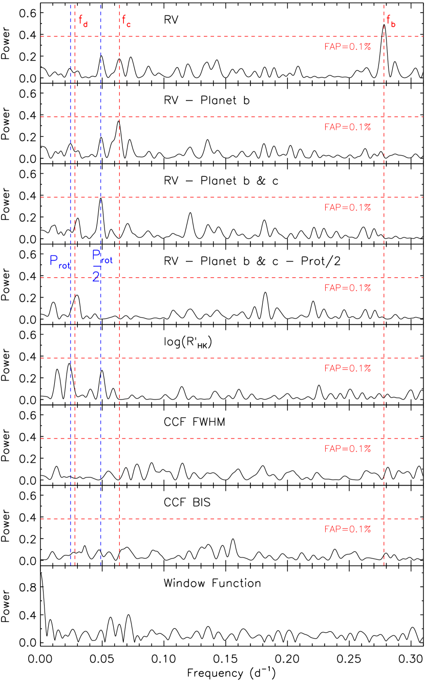
Figure 6: Generalized Lomb-Scargle periodogram of the 2019 HARPS measurements (upper panel) and RV residuals, following the subtraction of the Doppler signals of planet b (second panel), planets b and c (third panel), and planets b and c plus the 20.5 d signal (fourth panel). The periodogram of the Ca ii H & K lines activity indicator log R${}^{\prime}_{\mathrm{HK}}$, of the CCF BIS and FWHM, and of the window function are shown in the last four panels. The horizontal dashed lines mark the 0.1 % FAP. The orbital frequencies of planets b, c, and d, as well as the stellar rotation frequency and its first harmonic are marked with vertical dashed lines.

We computed the GLS periodogram of the RV residuals following the subtraction of the Doppler signal of EPIC 249893012 b. We fit the 2019 HARPS time series using the code pyaneti (Barragán et al., 2018, see also Sect. 6), assuming that planet b has a circular orbit, and kept both period and time of first transit fixed to the values derived from the K2 light curve, while allowing the RV semiamplitude to vary. The GLS periodogram of the RV residuals (Fig. 6, second panel) shows a peak at the orbital frequency of EPIC 249893012 c ($f_{\mathrm{c}}$ = 0.06 d^-1, $P_{\mathrm{c}}$ = 15.6 d) with an FAP $\approx$1 % over the frequency range 0.0–0.3 d^-1. Analogously, the FAP in a narrow spectral window centered around $f_{\mathrm{c}}$ = 0.06 d^-1 is $\sim$0.1 %.

We furthermore removed the RV signals of EPIC 249893012 b and c by performing a two-Keplerian joint fit to the HARPS data, assuming circular orbits and fixing periods and time of first transit to the K2 ephemeris. The GLS periodogram of the RV residuals, as obtained by subtracting the Doppler signals of the first two planets, displays a significant peak at $\sim$0.049 c/d (FAP $<$ 0.1 %), corresponding to a period of about 20.5 days (Fig. 6, third panel; see also next paragraph). We again subtracted this signal, along with the Doppler reflex motions of planets b and c, modeling the HARPS measurements with a sine curve and two circular Keplerian orbits. The periodogram of the RV residuals shows a peak close to the orbital frequency of the outer transiting planet EPIC 249893012 d ($f_{\mathrm{d}}$ = 0.028 d^-1; Fig. 6, fourth panel) whose FAP is, however, not significant (FAP $\approx$ 20 %) in the frequency domain 0.0–0.3 d^-1. The probability that random time series can produce a peak higher than the observed peak in a narrow window centered around the frequency of the outer transiting planet is $\sim$1 %.

The nature of the 20.5-day signal remains to be determined. The panels 5-7 of Fig. 6 display the periodogram of the Ca ii H & K lines activity indicator (log R${}^{\prime}_{\mathrm{HK}}$) and of the BIS and FWHM of the cross-correlation function, respectively. While the latter show no significant peaks at the orbital frequencies of the transiting planets or at 20.5 d ($\sim$0.049 c/d), the periodogram of log R${}^{\prime}_{\mathrm{HK}}$ displays a peak at 0.024 d^-1 ($P\,=\,41$ d), which is half the frequency (or twice the period) of the additional signal found in the RV residuals. The same periodogram also shows a peak at $\sim$0.049 d^-1 (20.5 d). Although none of the peaks seen in the periodogram of log R${}^{\prime}_{\mathrm{HK}}$ has an FAP ¡ 0.1 %, we suspect that the rotation period of the star is $P_{\mathrm{rot}}$ = 41 d, and that the signal at 20.5 d is the first harmonic of the rotation period, which might arise from the presence of active regions at opposite longitudes carried around by stellar rotation. Assuming that the star is seen equator-on, the stellar radius of $R_{\star}$ = 1.71 $\pm$0.04 $R_{\odot}$ and the projected rotation velocity of $V\sin i_{\star}$ = 2.1 $\pm$ 0.5 km s^-1 translate into a rotation period of 41 $\pm$ 10 d, corroborating our interpretation.

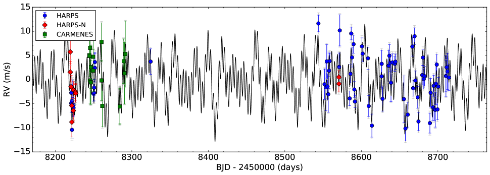
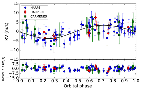
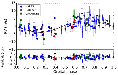
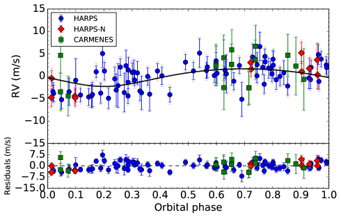
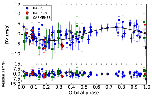
Figure 7: Top panel: Time series of the RV measurements of EPIC 249893012. Blue dots correspond to HARPS, red dots to HARPS-N, and green dots to CARMENES measurements. The best-fit model to the data is shown with a black thick line. The model includes three Keplerian curves and one sine curve mimicking the stellar signal at half the rotation period. Middle left panel: Phase-folded RV measurements over the period of planet b after removing the signals from planets c and d and stellar activity. Middle right panel: Phase-folded RV measurements over the period of planet c, after removing the signal from the other planets and stellar activity. Bottom left panel: Phase-folded RV measurements over the period of planet d, after subtracting the signal from planets b and c and stellar activity. Bottom right panel: Phase-folded RV measurements over half the rotation period of the star after removing the signals from the three planets.

6 Joint analysis

We simultaneously modeled the K2 transit photometry and HARPS, HARPS-N and CARMENES RV data with the software suite pyaneti (Barragán et al., 2019b), which uses Markov chain Monte Carlo (MCMC) techniques to infer posterior distributions for the fitted parameters. The RV measurements were modeled using the sum of three Keplerian orbits and a sine signal at half the rotation period of the star (see Sect. 5). The K2 transit light curves of the three planets were fit using the limb-darkened quadratic model of Mandel & Agol (2002). We integrated the light-curve model over ten steps to account for the 30 min integration time of K2 (Kipping, 2010). The fitted parameters are the systemic velocity $\gamma_{{\rm RV},i}$ for each instrument $i$, the RV semiamplitudes $K$, transit epochs $T_{0}$ and periods $P$ of the four Doppler signals, and the scaled semimajor axes $a/R_{\star}$, the planet-to-star radius ratios $R_{p}/R_{\star}$, the impact parameters $b$, the eccentricities $e$, the longitudes of periastron $\omega$, and the Kipping (2013) limb-darkening parametrization coefficients $q_{1}$ and $q_{2}$ for the three planets. We used the same expression for the likelihood as Barragán et al. (2016) and created 500 independent chains for each parameter, using informative priors from our individual stellar, transit, and RV analyses to optimize computational time. Adequate convergence was considered when the Gelman–Rubin potential scale reduction factor dropped to within 1.03. After finding convergence, we ran 25 000 more iterations with a thinning factor of 10, leading to a posterior distribution of 250 000 independent samples for each fit parameter.

The orbital parameters and their uncertainties from our photometric and spectroscopic best joint fit model, are listed in Table 3. They are defined as the median and 68% region of the credible interval of the posterior distributions for each fit parameter. The resulting RV time series and phase-folded planetary signals are shown in Fig. 7. All three planets are detected at higher than the 3 $\sigma$ level. The derived semiamplitudes for planets b, c, and d are 3.55${}^{+0.43}_{-0.43}$ m s^-1 , 3.66${}^{+0.45}_{-0.46}$ m s^-1, and 1.97${}^{+0.54}_{-0.47}$ m s^-1, respectively. The derived semiamplitude and period for the stellar activity signal are 3.20${}^{+0.46}_{-0.47}$ m s^-1 and 20.53${}^{+0.04}_{-0.04}$ days.

We also performed an independent joint analysis of our HARPS and HARPS-N RV and activity and symmetry indicator time series. We used the multidimensional Gaussian-process approach described by Rajpaul et al. (2015) as implemented in pyaneti by Barragán et al. (2019a). Briefly, this approach model RVs together with the activity and symmetry indicators assuming the same Gaussian process can describe them all following a quasi-periodic kernel. This approach has been used successfully to separate planet signals from stellar activity (e.g. Barragán et al., 2019a). The inferred Doppler semiamplitudes for the three planets are consistent within 1 $\sigma$ with the results presented in Table 3. We also found the period of the quasi-periodic (QP) kernel to be P${}_{\rm QP}\,=\,20.4\,\pm\,0.7$ d. This period comes from the correlation of the activity and symmetry indicators with the RV measurements, providing additional evidence that the $\sim$20-d RV signal is induced by stellar activity (see Sect. 5).

7 Discussion and conclusions

We reported on the discovery of three small planets ($R_{\mathrm{p}}<4$ $R_{\odot}$) transiting the evolved G8 IV/V star EPIC 249893012. Combining K2 photometry with high-resolution imaging and high-precision Doppler spectroscopy, we confirmed the three planets and determined their masses, radii, and mean densities. With an orbital period of 3.6 days, the inner planet b, has a mass of $M_{b}\,=\,8.75^{+1.09}_{-1.08}\,\ M_{\oplus}$ and a radius of $R_{b}\,=\,1.95^{+0.09}_{-0.08}\,\ R_{\oplus}$, yielding a mean density of $\rho_{b}\,=\,6.39^{+1.19}_{-1.04}$ g cm^-3. With an orbital period of 15.6 days, planet c has a mass of $M_{c}\,=\,14.67^{+1.84}_{-1.89}\ M_{\oplus}$ and a radius of $R_{c}=3.67^{+0.17}_{-0.14}\ R_{\oplus}$, yielding a mean density of $\rho_{c}=1.62^{+0.30}_{-0.29}$ g cm^-3. The outer planet d resides on a 35.7-day orbit, and has a mass of $M_{d}=10.18^{+2.46}_{-2.42}\,\ M_{\oplus}$ and a radius of $R_{d}\,=\,3.94^{+0.13}_{-0.12}\leavevmode\nobreak\ R_{\oplus}$, yielding a mean density of $\rho_{d}\,=\,0.91^{+0.25}_{-0.23}$ g cm^-3. For context, Figure 8 shows the mass-radius diagram for small planets with a mass and radius determination better than 30%. The three new planets reported in this paper are also shown.

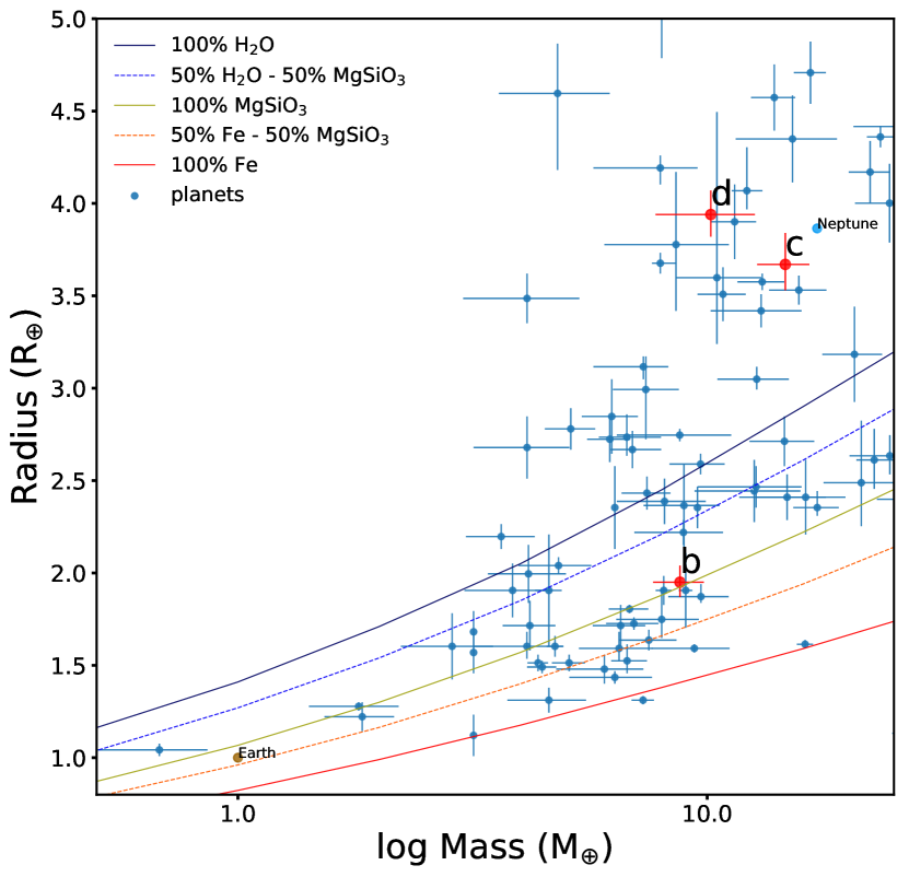
Figure 8: Mass vs. radius diagram for all known planets with masses in the range from 0.5 to 20.0 M_⊕ and radii from 0.8 to 5.0 R_⊕. Planets are shown only if the uncertainty in these two parameters is smaller than 30%. Data are retrieved from the NASA Exoplanet Archive (Akeson et al., 2013) as of September 2019. Theoretical models for internal composition of small planets are taken from (Zeng et al., 2016). The three planets we discovered and characterized in this paper are marked in red.

According to the Zeng et al. (2016) models, EPIC 249893012 b is a super-Earth with a density compatible with a pure silicate composition. However, a more realistic configuration would be a nickel-iron core and a silicate mantle. It lies above the model for 50% iron - 50% silicate, which probably means that it still has some residual H₂-He atmosphere, which enlarges its radius but does not significantly contribute to the total planet mass. As reported in Fulton et al. (2017) and Van Eylen et al. (2018), small planets follow a bimodal distribution with a valley at $\sim$1.5-2.2 $R_{\oplus}$ and peak at approximately 1.3 $R_{\oplus}$ for super-Earths and 2.4 $R_{\oplus}$ for sub-Neptunes. According to this, planet b, lies in the transition zone and might have lost most of its atmosphere through different mechanisms. The first is photoevaporation, which suggests a past atmosphere principally composed of hydrogen, which mainly occurs in the first 100 Myr of the stellar life, when it is more choromospherically active (Owen & Wu, 2013). On the other hand, Lee et al. (2014) proposed an alternative mechanism to explain a relatively thin atmosphere by delaying gas accretion into the planet until the gas in the protoplanetary disk is almost dissipated. Planetesimal impacts during planet formation can also encourage atmospheric loss (Schlichting et al., 2015), but it is unclear if impacts alone could produce the observed properties of planet b. Lopez & Rice (2018) suggested that RV follow-up of long-period planets found in surveys such as TESS (Ricker et al., 2015) or PLATO (Rauer et al., 2014) in the future should be able to distinguish between these two mechanisms because these two populations depend on semimajor-axis. Here, we estimate that given the proximity of planet b to its star ($\sim$0.05 AU), the influence of photoevaporation has been one of the most likely causes in the loss of its majority primordial hydrogen atmosphere.

EPIC 249893012 c and d are Neptune-sized planets, but with lower masses and hence lower mean densities (1.62 g cm^-3 and 0.91 g cm^-3 for planets c and d, respectively, vs. 1.95 g cm^-3 for Neptune), which suggest the presence of thicker atmospheres. Planet c has a stellar irradiation of $\sim$2.2$\cdot$10⁸ erg cm^-2 s^-1, that is, slightly above the threshold of 2$\cdot$10⁸ erg cm^-2 s^-1 established by Demory & Seager (2011), above which planets might inflate their atmospheres and be subject of photoevaporation. In contrast, planet d has a stellar irradiation of $\sim$7.2$\cdot$10⁷ erg cm^-2 s^-1 and should in principle not be subjected to photoevaporation processes. The radius of planet c may therefore be compared to models in Fortney et al. (2007) for gas giant planets, based on which, we derive a core mass of $\sim$10 $M_{\oplus}$. The density, radius and mass of planet d suggest a relatively small but heavy core with a thick atmosphere.

Based on the study of three planetary systems, Grunblatt et al. (2018) proposed that close-in planets orbiting evolved stars tend to reside on eccentric orbits. If this scenario is correct, the nearly circular orbits of EPIC 249893012 b, c, and d may be the result of the planets orbiting a star that is not evolved enough for a fair comparison to be made. According to the distance deduced in Table 3, we consider the three planets of the system EPIC 249893012 as close-in planets, with circular orbits, although for planet d a wide range of eccentricities from 0.04 to 0.36 is possible. Because the system is at an early stage of its evolution after leaving the main sequence, it is a good candidate for a detailed study of its dynamical evolution, to i) shed light on the formation of close-in giant planets (Dawson & Johnson, 2018), and ii) test the hypothesis by Izidoro et al. (2015) that giant planets form a dynamical barrier that confines super-Earths to an inward-migrating evolution.

Table 3: Parameters of the three planets and stellar signal from the joint-analysis fit.

Parameter	Planet b	Planet c	Planet d	Stellar signal
Transit and RV model parameters
Orbital period $P_{\textrm{orb}}\ (d)$	3.5951${}_{-0.0003}^{+0.0003}$	15.624${}_{-0.001}^{+0.001}$	35.747${}_{-0.005}^{+0.005}$	20.53${}_{-0.04}^{+0.04}$
Epoch $T_{0}$ (BJDTDB $-$ 2454833; d)	3161.396${}_{-0.005}^{+0.005}$	3165.841${}_{-0.004}^{+0.002}$	3175.652${}_{-0.003}^{+0.003}$	3263.72${}_{-0.95}^{+0.86}$
Scaled semimajor axis $a/R_{*}$	5.93${}_{-0.60}^{+0.96}$	15.79${}_{-2.56}^{+1.58}$	27.42${}_{-4.44}^{+2.74}$	…
Planet-to-star ratio radius $r_{p}/R_{*}$	0.0104${}_{-0.0004}^{+0.0004}$	0.0197${}_{-0.0006}^{+0.0008}$	0.0211${}_{-0.0004}^{+0.0005}$	…
Impact parameter $b$	0.42${}_{-0.25}^{+0.28}$	0.60${}_{-0.21}^{+0.15}$	0.25${}_{-0.17}^{+0.23}$	…
$\sqrt{e}\sin\omega_{*}$	-0.08${}_{-0.23}^{+0.24}$	-0.02${}_{-0.26}^{+0.25}$	-0.01${}_{-0.27}^{+0.29}$	0
$\sqrt{e}\cos\omega_{*}$	-0.04${}_{-0.16}^{+0.16}$	0.12${}_{-0.18}^{+0.12}$	-0.23${}_{-0.30}^{+0.29}$	0
Doppler semiamplitude $K\ (m\ s^{-1})$	3.55${}_{-0.43}^{+0.43}$	3.66${}_{-0.46}^{+0.45}$	1.97${}_{-0.47}^{+0.54}$	3.20${}_{-0.47}^{+0.46}$
Parameterized limb-darkening coefficient $q_{1}$	$0.43\pm 0.09$	…	…	…
Parameterized limb-darkening coefficient $q_{2}$	$0.22\pm 0.09$	…	…	…
Systemic velocity $\gamma_{\mathrm{HARPS}}\ (km\ s^{-1})$	21.6127${}_{-0.0003}^{+0.0003}$	…	…	…
Systemic velocity $\gamma_{\mathrm{HARPS-N}}\ (km\ s^{-1})$	21.6080${}_{-0.0009}^{+0.0009}$	…	…	…
Systemic velocity $\gamma_{\mathrm{CARMENES}}\ (km\ s^{-1})$	49.660${}_{-0.001}^{+0.001}$	…	…	…
RV jitter $\sigma_{\mathrm{HARPS}}\ (m\ s^{-1})$	1.40${}_{-0.42}^{+0.43}$	…	…	…
RV jitter $\sigma_{\mathrm{HARPS-N}}\ (m\ s^{-1})$	1.41${}_{-1.29}^{+0.95}$	…	…	…
RV jitter $\sigma_{\mathrm{CARMENES}}\ (m\ s^{-1})$	1.51${}_{-1.53}^{+1.05}$	…	…	…
Derived parameters
Planet radius $R_{\mathrm{p}}\ (R_{\oplus})$	1.95${}_{-0.08}^{+0.09}$	3.67${}_{-0.14}^{+0.17}$	3.94${}_{-0.12}^{+0.13}$	…
Planet mass $M_{\mathrm{p}}\ (M_{\oplus})$	8.75${}_{-1.08}^{+1.09}$	14.67${}_{-1.89}^{+1.84}$	10.18${}_{-2.42}^{+2.46}$	…
Planet density $\rho_{\mathrm{p}}\ (g\ cm^{-3})$	6.39${}_{-1.04}^{+1.19}$	1.62${}_{-0.29}^{+0.30}$	0.91${}_{-0.23}^{+0.25}$	…
Time of periastron passage ($d$)	3161.67${}_{-1.7}^{+1.2}$	3165.3${}_{-3.7}^{+4.4}$	3175.77${}_{-9.0}^{+7.9}$	…
Semimajor axis $a\ (AU)$	0.047${}_{-0.007}^{+0.005}$	0.13${}_{-0.02}^{+0.01}$	0.22${}_{-0.04}^{+0.02}$	…
Orbit inclination $i_{\mathrm{p}}$ $deg$	86.14${}_{-3.50}^{+2.60}$	87.94${}_{-1.05}^{+0.74}$	89.47${}_{-0.50}^{+0.36}$	…
Eccentricity $e$	0.06${}_{-0.04}^{+0.08}$	0.07${}_{-0.05}^{+0.08}$	0.15${}_{-0.11}^{+0.21}$	…
Longitude of periastron $\omega_{*}\ (^{\circ})$	225${}_{-123}^{+67}$	217${}_{-170}^{+100}$	181${}_{-61}^{+81}$	…
Transit duration $\tau_{14}\ (h)$	4.33${}_{-0.15}^{+0.18}$	6.37${}_{-0.12}^{+0.15}$	9.56${}_{-0.13}^{+0.14}$	…
Equilibrium temperature $T_{\textrm{eq}}\ (\textrm{K})$	1616${}_{-79}^{+149}$	990${}_{-49}^{+92}$	752${}_{-37}^{+69}$	…
Insolation $F\ (F_{\oplus})$	1037${}_{-207}^{+482}$	160${}_{-29}^{+68}$	53${}_{-10}^{+23}$	…

Table 4: HARPS measurements of EPIC 249893012.

BJDTDB	RV	eRV	CCFBIS	CCFFWHM	log RHK	elog RHK	S/N${}_{5500\,\AA}$	Texp	Instrument
(d)	(km s-1)	(km s-1)	(km s-1)	(km s-1)				(s)
2458220.78441	21.6078	0.0020	-0.0075	7.1754	-5.18	0.04	40.8	2400	HARPS
2458220.86371	21.6099	0.0017	-0.0089	7.1837	-5.19	0.03	48.9	2400	HARPS
2458221.78704	21.6083	0.0022	0.0004	7.1679	-5.16	0.04	37.2	2400	HARPS
2458221.85556	21.6023	0.0018	-0.0132	7.1876	-5.17	0.03	45.9	2400	HARPS
2458222.79324	21.6108	0.0018	-0.0009	7.1885	-5.17	0.03	44.1	2400	HARPS
2458222.84368	21.6106	0.0017	-0.0152	7.1921	-5.20	0.03	48.3	2400	HARPS
2458223.80514	21.6074	0.0021	-0.0058	7.1831	-5.17	0.04	40.0	2400	HARPS
2458223.89387	21.6068	0.0019	-0.0016	7.1926	-5.17	0.04	43.9	2400	HARPS
2458249.73305	21.6098	0.0016	-0.0051	7.1866	-5.18	0.03	50.3	2700	HARPS
2458250.74892	21.6110	0.0017	-0.0069	7.1858	-5.22	0.04	48.2	2400	HARPS
2458250.77753	21.6099	0.0017	-0.0047	7.1945	-5.15	0.03	48.7	2400	HARPS
2458251.77954	21.6163	0.0020	-0.0086	7.1831	-5.14	0.04	40.7	2400	HARPS
2458251.80647	21.6151	0.0029	0.0011	7.1821	-5.05	0.06	29.6	2400	HARPS
2458324.63972	21.6164	0.0026	-0.0053	7.1896	-5.25	0.07	32.4	2400	HARPS
2458543.86587	21.6243	0.0017	-0.0034	7.1865	-5.36	0.07	51.3	2400	HARPS
2458551.83867	21.6117	0.0032	-0.0072	7.1884	-5.23	0.09	30.6	2400	HARPS
2458553.80415	21.6111	0.0049	-0.0010	7.1938	-5.78	0.59	22.0	2400	HARPS
2458554.81840	21.6165	0.0035	0.0105	7.1750	-5.30	0.14	28.9	2400	HARPS
2458555.81881	21.6113	0.0026	-0.0087	7.1888	-5.58	0.17	36.6	2400	HARPS
2458556.79144	21.6097	0.0037	0.0036	7.1912	-5.20	0.11	27.0	2400	HARPS
2458557.82395	21.6145	0.0037	-0.0128	7.1781	-5.50	0.21	27.2	2400	HARPS
2458558.81788	21.6165	0.0017	-0.0082	7.1929	-5.27	0.05	53.2	2400	HARPS
2458570.90587	21.6153	0.0029	-0.0076	7.1910	-5.11	0.07	33.8	2700	HARPS
2458571.82537	21.6229	0.0032	-0.0043	7.1805	-5.15	0.08	30.8	2700	HARPS
2458584.78548	21.6088	0.0015	-0.0075	7.1924	-5.17	0.03	56.9	2400	HARPS
2458585.83025	21.6139	0.0019	-0.0041	7.1889	-5.16	0.04	45.9	2700	HARPS
2458586.77962	21.6222	0.0013	-0.0086	7.1878	-5.14	0.02	64.4	2700	HARPS
2458587.82822	21.6173	0.0020	0.0017	7.1815	-5.12	0.04	44.6	2400	HARPS
2458589.85191	21.6200	0.0019	-0.0116	7.1851	-5.12	0.03	46.2	2700	HARPS
2458590.82593	21.6106	0.0016	-0.0113	7.2020	-5.13	0.03	52.6	2700	HARPS
2458591.65814	21.6081	0.0013	-0.0178	7.2019	-5.17	0.02	64.3	2700	HARPS
2458600.79471	21.6196	0.0018	-0.0050	7.1874	-5.28	0.06	52.7	2700	HARPS
2458601.79254	21.6181	0.0016	-0.0014	7.2017	-5.29	0.05	57.7	2700	HARPS
2458608.68407	21.6171	0.0023	-0.0004	7.1847	-5.31	0.07	40.6	2700	HARPS
2458609.66596	21.6072	0.0022	-0.0021	7.1933	-5.16	0.05	42.9	2700	HARPS
2458613.81491	21.6031	0.0024	-0.0049	7.2012	-5.24	0.09	40.2	2700	HARPS
2458626.58042	21.6134	0.0025	-0.0071	7.1917	-5.11	0.04	34.7	2700	HARPS
2458626.61341	21.6159	0.0028	-0.0023	7.1932	-5.16	0.06	31.0	2700	HARPS
2458627.75972	21.6087	0.0025	-0.0102	7.1941	-5.37	0.12	39.0	2700	HARPS
2458635.65975	21.6156	0.0032	-0.0170	7.2012	-5.21	0.09	31.0	2700	HARPS
2458636.64443	21.6176	0.0023	-0.0094	7.2018	-5.26	0.07	39.8	2700	HARPS
2458637.75899	21.6162	0.0018	-0.0058	7.1791	-5.34	0.07	51.0	2700	HARPS
2458638.73082	21.6120	0.0039	0.0075	7.1803	-5.16	0.13	27.6	2700	HARPS
2458640.73000	21.6162	0.0018	-0.0004	7.1927	-5.19	0.05	52.3	2700	HARPS
2458643.69045	21.6159	0.0016	-0.0064	7.1887	-5.42	0.08	58.5	2400	HARPS
2458644.65679	21.6164	0.0016	-0.0049	7.1905	-5.19	0.05	56.7	2400	HARPS
2458655.67055	21.6086	0.0048	0.0051	7.1902	-4.87	0.06	21.0	2400	HARPS
2458657.68053	21.6025	0.0026	-0.0061	7.1712	-5.12	0.05	35.0	2400	HARPS
2458660.63404	21.6054	0.0026	-0.0008	7.1882	-5.08	0.05	34.5	2400	HARPS
2458666.62842	21.6195	0.0020	-0.0119	7.1968	-5.12	0.04	44.5	2400	HARPS
2458667.63837	21.6109	0.0017	-0.0065	7.1932	-5.13	0.03	52.4	2700	HARPS
2458669.62253	21.6217	0.0018	-0.0032	7.1965	-5.17	0.03	49.4	2400	HARPS
2458670.63466	21.6125	0.0020	-0.0093	7.1995	-5.13	0.04	44.1	2400	HARPS
2458673.63051	21.6090	0.0023	-0.0076	7.1913	-5.14	0.04	38.4	2680	HARPS
2458674.64597	21.6040	0.0019	-0.0087	7.1856	-5.17	0.04	46.6	2400	HARPS
2458679.62480	21.6136	0.0021	-0.0091	7.2000	-5.56	0.17	47.3	2400	HARPS
2458680.61023	21.6173	0.0017	-0.0058	7.1990	-5.34	0.07	54.3	2400	HARPS
2458681.62554	21.6128	0.0021	-0.0133	7.1888	-5.27	0.07	46.2	2400	HARPS
2458682.60541	21.6134	0.0020	-0.0083	7.1965	-5.27	0.06	45.6	2400	HARPS
2458689.62388	21.6037	0.0021	-0.0065	7.1943	-5.33	0.10	46.1	2400	HARPS
2458690.57672	21.6099	0.0030	-0.0036	7.1948	-5.31	0.11	32.8	2400	HARPS
2458693.54664	21.6069	0.0027	-0.0129	7.1939	-5.22	0.09	36.0	2400	HARPS
2458694.59633	21.6114	0.0022	-0.0027	7.1935	-5.29	0.07	43.0	2400	HARPS
2458695.58627	21.6065	0.0023	-0.0130	7.1918	-5.54	0.13	41.5	2400	HARPS
2458696.57103	21.6064	0.0036	0.0020	7.2044	-5.44	0.21	29.7	2400	HARPS
2458697.59484	21.6118	0.0043	-0.0039	7.1721	-5.84	0.74	25.6	2400	HARPS
2458698.61455	21.6158	0.0021	-0.0093	7.1924	-5.24	0.07	44.7	2400	HARPS
2458699.57794	21.6065	0.0022	-0.0125	7.1905	-5.33	0.09	44.2	2400	HARPS
2458700.56352	21.6112	0.0019	-0.0093	7.1829	-5.41	0.08	48.1	2400	HARPS
2458711.50542	21.6153	0.0019	0.0008	7.1904	-5.36	0.08	49.6	2400	HARPS
2458712.52173	21.6144	0.0038	-0.0275	7.1965	-5.55	0.27	28.3	2400	HARPS
2458714.47713	21.6131	0.0027	-0.0094	7.1841	-5.14	0.07	36.5	2100	HARPS

Table 5: HARPS-N measurements of EPIC 249893012.

BJDTDB	RV	eRV	CCFBIS	CCFFWHM	log RHK	elog RHK	S/N${}_{5500\,\AA}$	Texp	Instrument
(d)	(km s-1)	(km s-1)	(km s-1)	(km s-1)				(s)
2458219.63943	21.6138	0.0024	-0.0087	7.1193	-5.11	0.05	38.1	2700	HARPS-N
2458219.67084	21.6096	0.0023	-0.0173	7.1197	-5.15	0.05	40.6	2700	HARPS-N
2458220.64565	21.6066	0.0024	-0.0083	7.1229	-5.11	0.05	39.1	2700	HARPS-N
2458221.63935	21.6026	0.0037	-0.0157	7.1333	-5.14	0.09	27.9	2600	HARPS-N
2458221.66954	21.5992	0.0031	-0.0114	7.1269	-5.18	0.08	31.8	2600	HARPS-N
2458223.61735	21.6016	0.0020	-0.0069	7.1224	-5.19	0.05	45.2	2400	HARPS-N
2458223.64464	21.6059	0.0017	-0.0069	7.1208	-5.16	0.04	50.2	2400	HARPS-N
2458226.60910	21.6055	0.0017	-0.0134	7.1246	-5.17	0.03	50.3	1800	HARPS-N
2458226.62995	21.6052	0.0018	-0.0163	7.1258	-5.19	0.04	48.2	1800	HARPS-N
2458570.66046	21.6085	0.0014	-0.0149	7.1242	-5.16	0.02	62.4	3600	HARPS-N
2458570.70977	21.6072	0.0017	-0.0120	7.1222	-5.20	0.04	51.7	3600	HARPS-N

Table 6: CARMENES measurements of EPIC 249893012.

BJDTDB	RV	eRV	CCFBIS	CCFFWHM	log RHK	elog RHK	S/N${}_{5340\,\AA}$	Texp	Instrument
(d)	(km s-1)	(km s-1)	(km s-1)	(km s-1)				(s)
2458244.52311	49.6652	0.0045	-0.0132	7.7551	–	–	59.9	1800	CARMENES
2458244.54617	49.6651	0.0044	-0.0079	7.7543	–	–	59.6	1800	CARMENES
2458245.51467	49.6667	0.0050	0.0026	7.7540	–	–	53.6	1800	CARMENES
2458245.53632	49.6600	0.0049	-0.0253	7.7772	–	–	56.5	1800	CARMENES
2458246.50860	49.6596	0.0046	-0.0458	7.7732	–	–	58.8	1800	CARMENES
2458246.53124	49.6627	0.0045	-0.0338	7.7594	–	–	60.8	1800	CARMENES
2458249.53854	49.6620	0.0044	-0.0081	7.7522	–	–	62.1	1800	CARMENES
2458249.56019	49.6649	0.0047	-0.0248	7.7298	–	–	58.0	1800	CARMENES
2458260.50626	49.6600	0.0042	-0.0310	7.7646	–	–	64.2	1800	CARMENES
2458260.52919	49.6680	0.0040	-0.0256	7.7473	–	–	67.5	1800	CARMENES
2458261.48996	49.6547	0.0044	-0.0183	7.7661	–	–	60.3	1800	CARMENES
2458284.43860	49.6546	0.0036	-0.0222	7.7784	–	–	75.8	1800	CARMENES
2458284.46094	49.6546	0.0037	-0.0389	7.7531	–	–	71.8	1800	CARMENES
2458289.40632	49.6640	0.0046	-0.0244	7.7711	–	–	59.8	1800	CARMENES
2458290.42667	49.6615	0.0064	0.0080	7.7874	–	–	44.2	1800	CARMENES
2458291.44303	49.6655	0.0068	-0.0469	7.7647	–	–	41.2	1800	CARMENES