Modern Concepts of Quantum Equilibration Do Not Rule Out Strange Relaxation Dynamics

Abstract

Numerous pivotal concepts have been introduced to clarify the puzzle of relaxation and/or equilibration in closed quantum systems. All of these concepts rely in some way on specific conditions on Hamiltonians $H$, observables $A$, and initial states $\rho$ or combinations thereof. We numerically demonstrate and analytically argue that there is a multitude of pairs $H,A$ that meet said conditions for equilibration and generate some ”typical” expectation value dynamics which means, $\langle A(t)\rangle\propto f(t)$ approximately holds for the vast majority of all initial states. Remarkably we find that, while restrictions on the $f(t)$ exist, they do not at all exclude $f(t)$ that are rather adverse or “strange” regarding thermal relaxation.

I Introduction

Since the beginning of the previous century, numerous concepts have been suggested to account for the emergence of irreversible thermodynamics from the underlying, reversible unitary quantum dynamics Gogolin and Eisert (2016). Despite its long history, this is an active field of research, even to date. With the paper at hand we intend to show that, while all these concepts are certainly cornerstones of our understanding of the origins of the second law, they are not yet sufficient to rule out certain types of dynamics of observables that may be perceived a being at odds with the arrow of time and which we address as “strange dynamics”. But before embarking on a detailed demonstration of their existence, we first name some valuable approaches to equilibration in closed quantum systems which nonetheless fail to exclude said strange dynamics. This list is neither intended to be complete nor to serve as a full fledged introduction to the subject, readers well acquainted with its items may skip it.

equilibration on average: Statement on temporal fluctuations of e.g., expectation values. Let the Hamiltonian $H$ with $H\ket{\epsilon_{j}}=\epsilon_{j}\ket{\epsilon_{j}}$ have a sufficiently low number of equal energy gaps $\epsilon_{i}-\epsilon_{j}$ (“non-resonance condition”). Let furthermore the “effective dimension” $d_{\text{eff}}:=(\sum_{j}\bra{\epsilon_{j}}\rho\ket{\epsilon_{j}}^{2})^{-1}$ with $\rho$ being the initial state, be large, i.e., $d_{\text{eff}}\gg 1$. Then excursions of an expectation value $\langle A(t)\rangle$ from some “equilibrium value” $A_{\text{eq}}:=\int_{0}^{T}\langle A(t)\rangle\text{d}t/T$ are rare in the sense that $(\langle A(t)\rangle-A_{\text{eq}})^{2}\ll||A||$ for most $t$ from $[0,T]$ Reimann (2008); Short and Farrelly (2012); Linden et al. (2009).

eigenstate thermalization hypothesis (ETH): Assumption on $H,A$, more precisely on random number-like properties of matrix elements $A_{ij}:=\bra{\epsilon_{i}}A\ket{\epsilon_{j}}$, see also Eq. (2). The applicability of the ETH ensures the above rareness of excursions from equilibrium and a fixed $A_{\text{eq}}$ for all initial states from some energy shell (“thermalization”). The validity of the ETH is closely related to quantum chaos, cf. corresponding item below. Srednicki (1994); Deutsch (1991).

typicality: Statistical statement on properties of pure states. Let the dimension of some finite Hilbertspace $d$ be large, $d\gg 1$. Let $A$ be an operator on this Hilbertspace with a spectral variance of order unity. Furthermore $|\psi\rangle$ are pure states that drawn at random according to the unitary invariant Haar-measure from this Hilbert space. Then, for the overwhelming majority of all $|\psi\rangle$, the expectation values $\langle\psi|A|\psi\rangle$ are very close to $\Tr{A}/d$ Lloyd (2013); Reimann (2007); Reimann and Gemmer (2019a); Popescu et al. (2006); Linden et al. (2009); Tasaki (2016); Sugiura and Shimizu (2013); Goldstein et al. (2006). In the absence of of any further information on $|\psi\rangle$ it is thus rational to assume $\langle\psi|A(t)|\psi\rangle\approx\Tr{A}/d$, independent of $t$.

quantum chaos: An observable featuring a finite overlap with a conserved quantity cannot relax to an equilibrium value independently of its initial value Mazur (1969). Wigner-Dyson-type (rather than Poissonian) statistics of spacings of adjacent energy eigenvalues signal the absence of many nontrivial conserved quantities (“integrability”) Haake (1991).

microreversibility: Principal property of the dynamics of a system that ensures that an operation like flipping of particle momenta indeed entails a kind of reversed dynamics. Fluctuation relations, which are often viewed as more detailed formulations of the second law, are routinely based on microreversibility Campisi et al. (2011). While the abstract concept is more encompassing, a version of microreversibility is implemented if $A,H$ are both real in a common basis, cf. Eq. (2).

nonfine-tuned initial states: Some specific mathematical constructions of initial states $\rho$ obviously allow for implementing dynamics that are at odds with regular thermal relaxation. Thus a non-trivial conflict with the arrow of time requires the occurrence of strange relaxation dynamics for nonfine-tuned initial states, i.e., states that do not require: backwards evolving of non-equilibrium states, flipping of particle momenta or complex conjugating of wave-functions $|\psi(t)\rangle\rightarrow|\psi(t)\rangle^{*}$ (no “Loschmidt-operations”), full control over each individual matrix element $\bra{\epsilon_{i}}\rho\ket{\epsilon_{j}}$, etc. Campisi et al. (2011)

This article is organized as follows: In section II we elaborate on what is meant by ”strange dynamics” and formulate our main claim. In section III we present numerical examples of ”strange dynamics” that back up our main claim and explain how the numerical construction of these examples works. The physical relevance of the respective initial states underlying these dynamics is discussed in section IV. In section V we analytically argue for the validity of the main claim for (mixed) initial states that commute with the observable. These arguments suggest that the main claim is valid in the limit of large systems, which is supported by a numerical finite-size-scaling in section VI. In section VII we generalize the result on certain classes of pure initial states that do not commute with the observable.

II Notion of strange dynamics and main claim

Prior to stating the main claim of the paper at hand we first establish the notion of ”strange dynamics”: To comply with equilibration on average the considered expectation value $\Tr{A(t)\rho}:=\langle A(t)\rangle$ must take a fixed value $A_{\text{eq}}$ for the vast majority of all instances in time. It may, however, nevertheless exhibit a behavior which is entirely unexpected in the context of relaxation dynamics. It could, e.g., follow the contour of some skyline before settling to $A_{\text{eq}}$, cf. Fig 1. Or it could, after having seemingly settled to $A_{\text{eq}}$, spike to a significantly off-equilibrium value at a time long compared to its initial relaxation time but much shorter than the Poincare recurrence time, cf. Fig 2. Any such unexpected dynamics we call ”strange dynamics” without further rigorous definition.

Our main claim is as follows: It is possible to find a multitude of pairs $H,A$ in accord with all above equilibration principles such that

$$\langle A(t)\rangle\approx\langle A(0)\rangle f(t)\quad(f(0)=1)$$ (1)

where $f(t)$ must have a positive Fourier transform. Other than that $f(t)$ may essentially be freely chosen. Among the possible choices are plenty of strange dynamics, cf. Figs. 1, 2. Most importantly the validity of Eq. (1) is claimed for a vast majority of all initial states $\rho$. This major set of initial states will be detailed below, see Sects. V, VII.

This claim is the more technical reformulation of the central statement which forms the title of the present paper. (For some numerical evidence of the validity of Eq. (1) in concrete spin systems, albeit with non-strange $f(t)$’s, see Ref. Richter et al. (2019))

III Making of Figures 1 and 2: Hamiltonians, Observables and Initial States

Figs. 1, 2 show various expectation value dynamics as resulting from the solution of the Schrödinger equation for fixed $H,A$ (per panel in Fig. 1) but various $\rho$. The somewhat odd examples in Fig. 1 have simply been picked to substantiate the above claim that $f(t)$ may essentailly be chosen at will, cf. Eq. (1). The setting in Fig. 2 is meant as a prime example of strange dynamics in the sense described above. Of course peculiar dynamics as presented in Figs. 1, 2 require pairs $H,A$ with specific properties. In the following we detail the construction of $H,A$, thereby unveiling their accordance with the cornerstone principles of thermal relaxation.

First a $d$-dimensional Hamiltonian $H$ is defined by choosing $d$ eigenvalues $\epsilon_{j}$ (examples in Figs. 1, 2: $d=20000$). To this end $d-1$ energy-gaps $l_{j}=\epsilon_{j+1}-\epsilon_{j}$ are drawn as i.i.d. random numbers from a pertinent Wigner-Dyson distribution. The spectrum is scaled to span an interval $[-E,E]$ (examples in Figs. 1, 2: $E=30$). Within this interval $H$ has thus a constant density of states and exhibits Wigner-Dyson level statistics as expected for non-integrable systems. Thus our modeling is in accord with the non-resonance condition and quantum chaos in the sense of the respective items in the introductory list in Sect. I. This Hamiltonian $H$ may be viewed as the sector of a, e.g., many-body Hamiltonian that corresponds to a (narrow) energy window stretching from $-E$ to $E$. If the initial state lives (almost) entirely in this energy window, which is what we assume here, modeling of this sector suffices to compute the dynamics. Note that $\langle A(t)\rangle$ is fully determined by the spectra and the ”relative angles” of the eigenvectors of the operators $H,A,\rho$. Thus, there is no need to specify the eigenvectors of $H$ with respect to some ”computational basis” for the purposes at hand.

Next we construct the observables $A$. To this end we first define $\tilde{f}(\omega)$ to be the real part of the Fourier transform of some desired, possibly strange, $f(t)$. Let furthermore $\omega_{\text{max}}$ be some “cut-off frequency” $\omega_{\text{max}}$, such that $\tilde{f}(\omega)$ attains only negligible values at $|\omega|\geq\omega_{\text{max}}$. Choose $E,\omega_{\text{max}}$ such as to fulfil $E\gg\omega_{\text{max}}$ (examples in Figs. 1, 2: $\omega_{\text{max}}\approx 3$). Furthermore $\tilde{f}(\omega)$ has to vary only negligibly on the scale of the level-spacings $l_{j}$. While these conditions on $\tilde{f}(\omega)$ imply conditions on $f(t)$, these conditions become exeedingly mild, at sufficiently large $d$.

Now we specify the $A$’s in the energy eigenbasis $\{\ket{\epsilon_{i}}\}$ in full accord with the ETH Srednicki (1999) as

$${A}_{jl}:=\bra{\epsilon_{j}}A\ket{\epsilon_{l}}=C_{1}d^{-1/2}\sqrt{\tilde{f}(\epsilon_{j}-\epsilon_{l})}\,R_{jl}\ ,$$ (2)

where $R_{jl}$ are normally i.i.d. random real numbers with zero mean and unit variance. $C_{1}$ is a constant which we use to scale the extreme eigenvalues of $A$ to $|a_{\text{min}}|\approx|a_{\text{max}}|\approx 1$. To render $A$ Hermitian, $\tilde{f}(\omega)$ must be nonnegative which implies the condition on $f(t)$ mentioned below Eq (1). To support our main claim it suffices that $A$ as defined in Eq. (2) is not in conflict with the ETH. But what is more, numerous numerical studies found operators of local observables (currents, magnetizations, etc.) in the eigenbasis’ of the respective Hamiltonians (many-body lattice models) to essentially agree with the construction Eq. (2) D’Alessio et al. (2016); Beugeling et al. (2015); Mondaini and Rigol (2017); Mukerjee et al. (2006); Kolovsky and Buchleitner (2004); Parra-Murillo et al. (2014); Torres-Herrera et al. (2016); Nation and Porras (2018); Mondaini et al. (2018); Hamazaki and Ueda (2019); Foini and Kurchan (2019), for more details see App. A. Choosing the ${A}_{jl}$ real renders the set-up microreversible in the sense defined in the respective item of the introductory list of equilibration principles .

Ultimately we aim at establishing that this construction of $H,A$ renders Eq. (1) valid for practically all nonfine-tuned initial states $\rho$. However, for the numerical demonstration of this validity as displayed in Figs. 1, 2, we chose initial states from the following two classes:

observable eigenstates: Let $|a_{j}\rangle$ be an eigenstate of $A$, i.e., $A|a_{j}\rangle=a_{j}|a_{j}\rangle$. The dynamics in Figs. 1, 2 (upper panel) are computed for some sample initial eigenstates of $A$, i.e., $\rho=|a_{j}\rangle\langle a_{j}|$ for eigenvalues $a_{j}$ which may be inferred from the respective captions.

unbiased ensemble states: The dynamics in Fig. 2 (lower panel) correspond to states $\rho=|\psi\rangle\langle\psi|$ with

$$\ket{\psi}=\bra{\phi}\ket{\phi}^{-1/2}\ket{\phi},\quad\ket{\phi}=(1+\lambda A)^{-1/2}\ket{\xi}$$ (3)

where $\ket{\xi}$ is a random vector unitarily drawn from the $d$-dimensional hypersphere in Hilbertspace. $\lambda$ has been chosen such as to obtain the respective $\langle A(0)\rangle$ as indicated in the caption of Fig. 2.

Before motivating the above choice of initial states we provide some more information on Figs. 1, 2. For Fig. 1 the functions $f(t)$ have been extracted from the respective underlying pictures. (The pictures and contours have been chosen such as to make sure that the contours indeed feature positive Fourier transforms.) For Fig. 2 $f(t)$ is simply a pertinent mathematical function, the revival time $\tau_{R}$ of which is chosen as $\tau_{R}=10$, which is much longer than the timescale of the initial decay but definitely much shorter than the Poincare recurrence time, cf. B, making this example a prime instance of strange dynamics. The respective $H,A$ have been constructed according to the above scheme. The respective Schrödinger equations have been numerically solved for the sample initial states as described above and in the captions. Obviously all computed data are in excellent agreement with our main claim, Eq. (1). (Even more numerical support for the latter comes from the data displayed in Fig 3). All initial states feature effective dimensions of at least $d_{\text{eff}}\geq 4700$, i.e., are in accord with the principle of equilibration on average, for more detailed information see App. C.

Figure 1: $H$ and $A$ may be tailored such that $\langle A(t)\rangle/\langle A(0)\rangle$ follows almost any desired function $f(t)$ for a majority of initial states. Displayed data are for initial states that are eigenstates of $A$, i.e., $A|\psi(0)\rangle=a_{j}|\psi(0)\rangle$. Green and red symbols: $\langle A(t)\rangle/\langle A(0)\rangle$, blue line: desired function $f(t)$.
(a) Burj Khalifa (original photo: ”Burj Khalifa” by Joi is licensed under CC BY 2.0, https://commons.wikimedia.org), (b) Bitcoin price, (c) elephants (original photo: ”Family Of Elephants” by Javier Puig Ochoa is licensed under CC BY 3.0, https://commons.wikimedia.org)

Figure 2: $\langle A(t)\rangle$ exhibits a significant revival at an arbitrary predefined time $\tau_{R}$ (here $\tau_{R}=10$) for two classes of initial states: (a) $|\psi(0)\rangle$ are eigenstates of $A$, (b) $|\psi(0)\rangle$ are samples of an unbiased pure state ensemble conditioned on a given $\langle A(0)\rangle$, cf. Eq. (3)

IV Physical Significance of the initial states underlying the displayed data

Before explaining the inner workings of the above construction of $H,A$ we comment on the physical significance of the initial states used in Figs. 1, 2. Some physical relevance of the initial observable eigenstates $|a_{j}\rangle$ comes from their being identical to results of (preparatory) projective measurements of the monitored observable $A$ at the beginning of the relaxation dynamics. More importantly, however, the validity of Eq. (1) for $\rho=|a_{j}\rangle\langle a_{j}|$ for all $j$ necessarily entails the validity of Eq. (1) also for all initial states of the form $\rho=\sum_{n}c_{n}A^{n}$. The latter comprises e.g. $\rho\propto\exp^{\lambda A}$, which is the state of maximum von-Neumann entropy conditioned on some given $\langle A(0)\rangle$. This is a relevant class of initial states within the framework of Jayne’s principle.

The states from the unbiased ensemble, cf. Eq. (3) represent an ensemble of pure states which is entirely unbiased with respect to the unitary invariant Haar-measure, under the condition of a given $\langle A(0)\rangle$ Fine (2009); Müller et al. (2011); Reimann and Gemmer (2019b). This ensemble thus is a very relevant class of initial states within the framework of pure state statistical mechanics.

V Validity of the main claim (Equation (1)) for initial states which commute with the observable

In the following we explain why the above construction yields pairs $H,A$ that render our main claim Eq. (1) valid for the above mentioned class of initial states $\rho=\sum_{n}c_{n}A^{n}$ that also comprises the observable eigenstates $|a_{j}\rangle\langle a_{j}|$. Consider the relation

$$\Tr{{A}(t){A}^{N}}\approx\left\{\begin{array}[]{ll}\propto\Tr{{A}(t){A}}\propto f(t)\,,&\text{odd }N\\ 0\,,&\text{even }N\end{array}\right.\,.$$ (4)

Obviously the validity of this relation entails the validity of Eq. (1) for all initial states of the above class. Accordingly Eq. (4) is the first pillar on which Eq. (1) rests. The validity of a subpart of Eq. (4), namely $\Tr{{A}(t){A}}\propto f(t)$ follows rather straightforward from Eq. (2) (for details see App. D). To fully validate Eq. (4) we employ a scheme suggested in Ref. Richter et al. (2019). As the argument is quite involved for large exponents $N$, we here restrict ourselves to $N=2$ and $N=3$. A comparable but more complex derivation for arbitrary but fixed $N$ at large $d$ can be found in App. E.

We start by writing out the correlation function for $N=2$ explicitly,

$$\Tr{{A}(t){A}^{2}}=\sum_{a,b,c}{A}_{ab}A_{bc}{A}_{ca}\,e^{\imath(\epsilon_{b}-\epsilon_{a})t}\ .$$ (5)

Given the matrix structure in Eq. (2), the biggest part of the addends in the sum are by construction (products of) independent random numbers with zero mean. Thus, to an accuracy set by the law of large numbers, summing the latter yields zero as well. There are, however, index combinations for which not all factors within the addends have vanishing mean, namely, $c=a$. Focusing on these terms, we can write

$$\Tr{{A}(t){A}^{2}}\approx\!\!\sum_{a,b}|{A}_{ab}|^{2}{A}_{aa}e^{\imath(\epsilon_{b}-\epsilon_{a})t}\,.$$ (6)

While the numbers $|A_{ab}|^{2}$ do not have mean zero, the numbers $A_{aa}$ do have zero mean. Furthermore for $a\neq b$ the $|A_{ab}|^{2},{A}_{aa},e^{\imath(\epsilon_{b}-\epsilon_{a})t}$ are mutually independent stochastic variables, cf. Eq. (2). For $a=b$ these numbers are obviously not independent, however, in this case the sum in Eq. (6) is proportional to the third moment of the distribution of the $A_{aa}$ which vanishes according to Eq. (2). Exploiting these findings for both cases ($a\neq b$ as well as $a=b$) to evaluate Eq. (6) we obtain $\Tr{{A}(t){A}^{2}}\approx 0$, i.e., Eq. (4) for the even case $N=2$.

Now we turn to $N=3$, i.e.,

$$\Tr{{A}(t){A}^{3}}=\!\!\sum_{a,b,c,d}{A}_{ab}{A}_{bc}{A}_{cd}{A}_{da}e^{\imath(\epsilon_{b}-\epsilon_{a})t}\,.$$ (7)

Again, the contributions of most addends approximately cancel each other upon summation. But also here, there are exceptions, namely, the index combinations $c=a$ or $d=b$. Focusing on these terms, we find

$$\Tr{{A}(t){A}^{3}}\approx\!\!\sum_{a,b}(|{A}_{ab}|^{2}\sum_{c}|{A}_{bc}|^{2}+|{A}_{ac}|^{2})e^{\imath(\epsilon_{b}-\epsilon_{a})t}\,.$$ (8)

(Note that Eq. (8) erroneously counts the terms corresponding to $c=a$ and $d=b$ twice. However, as this over-counting error is of order $d^{-1}$, it becomes negligible at large $d$.) To proceed, consider the above sums over $c$ first. While these sums do not vanish, they are practically independent of $a,b$, due to the specific matrix structure of $A$, cf. Eq. (2). Thus, the respective sums may be replaced by a constant $C_{2}$, i.e., $\sum_{c}|A_{bc}|^{2}+|{A}_{ac}|^{2}\approx C_{2}$. Inserting this into Eq. (8) yields $\Tr{{A}(t){A}^{3}}\approx C_{2}\cdot\sum_{a,b}|{A}_{ab}|^{2}e^{\imath(\epsilon_{b}-\epsilon_{a})t}$. Comparing this to the exact relation $\Tr{{A}(t){A}}=\sum_{a,b}|{A}_{ab}|^{2}e^{\imath(\epsilon_{b}-\epsilon_{a})t}$ yields $\Tr{{A}(t){A}^{3}}\approx C_{2}\,\Tr{{A}(t)A}$, i.e., Eq. (4) for the odd case $N=3$.

VI Accuracy of the main claim (Equation (1)) for eigenstates of the observable as initial states

Mainly due to the neglect of terms with random signs (cf. below Eq. 5), Eq. (4) is not exact. To scrutinize the accuracy of Eq. (4) and hence Eq. (1) specifically with respect to growing dimensions $d$, the Schrödinger equation has been solved for the set-up underlying Fig. 1, panel (a), for all $|a_{j}\rangle$ (d =7000) respectively every 10th $|a_{j}\rangle$ (d=50 000) as initial states. Figure 3 shows the deviations from Eq. (1) at an exemplary point in time, here chosen as $t=10$. These deviations are defined as

$$D_{a_{j}}^{t}:=\langle a_{j}|A(t)|a_{j}\rangle-a_{j}f(t).$$ (9)

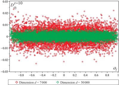
Figure 3: The mean values of the errors and the variances are almost independent of the eigenstate, which served as the respective initial state.

The errors have vanishing mean and a standard deviation that is almost independent of $a_{j}$. But, most importantly, the standard deviation decreases with the dimension $d$.

To numerically analyze this dependence, we consider the mean square of these errors (averaged over all eigenstates $a_{j}$ and over time):

$$\tensor{*}[]{D}{{}_{d}}=\frac{1}{d}\sum_{j=1}^{d}\frac{1}{T}\int_{0}^{T}\left(\tensor{*}[]{D}{{}^{t}_{a_{j}}}\right)^{2}\mathrm{d}t,\quad T=13$$ (10)

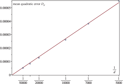
Figure 4: The finite-size scaling of the mean square of the errors $D_{d}$ indicates that these are proportional to $\frac{1}{d}$.

Plotting $D_{d}$ over the reciprocal Hilbertspace dimension $1/d$ (see Fig. 4) reveals that the mean square of these errors vanishes as $\propto d^{-1}$. This is supported by an analytical reasoning (see App. E). These findings imply that Eq. (1) becomes exact in the limit of large $d$ for all initial states of the form $\rho=\sum_{n}c_{n}A^{n}$, i.e., all initial states that commute with the observable $A$.

VII Validity of the main claim (Equation (1)) for a class of initial states which do not commute with the observable

Next we establish the validity of Eq. (1) for a set of (pure) initial states that are not of the form $\rho=\sum_{n}c_{n}A^{n}$, i.e., not functions of the observable $A$, and comprises the unbiased ensemble states (cf. Eq. (3)). We call this set the “$r$-set” and define its states $\ket{\eta}$ by

$$\ket{\eta}=\bra{\chi}\ket{\chi}^{-1/2}\ket{\chi},\quad\ket{\chi}=\sqrt{r(A)}\ket{\xi}$$ (11)

where $r(A)$ is a nonnegative function that varies little on the scale of the eigenvalue spacings of $A$ and $\ket{\xi}$ is a random vector drawn from the unitary invariant Haar-measure. Typicality arguments may be used to show that for all $\ket{\eta}$, except for a fraction of at most $\propto d^{-1/2}$ the approximation

$$\bra{\eta}A(t)\ket{\eta}\approx\Tr{r(A)A(t)}\Tr{r(A)}^{-1}$$ (12)

holds to very good accuracy. For a complete derivation see, Reimann and Gemmer (2019b) and App. F. As $r(A)$ may be cast into the form $r(A)=\sum_{n}b_{n}A^{n}$, the combination of Eqs. (12) and (4) establishes the validity of Eq. (1) for all $\ket{\eta}$ except for the above fraction of size $\propto d^{-1/2}$. Thus Eq. ((12) is the second pillar on which Eq. (1) rests. For the special case $r(A)=(1+\lambda A)^{-1}$ the $r$-set is identical to the unbiased ensemble, cf. Eq. (3), hence Eq. (12) explains the numerical findings displayed in Fig. 2 (lower panel). Note that the $r$-sets are very encompassing. The small fraction of order $d^{-1/2}$ of initial states that does not comply with Eq. (12) for a suitable $r(A)$ thus corresponds to the set of fine tuned initial states which always exist but are excluded from the analysis at hand, c.f. last item of the introductory list of principles of equilibration. Note furthermore that the validity of Eq. (12) entails the validity of Eq. (1) for all initial states of the form $\rho=\int g(\eta)\ket{\eta}\bra{\eta}$d$\eta$ with $g(\eta)\geq 0$ for the few (fine tuned) $\eta$ to which Eq. (12) does not apply. Thus Eq. (1) also holds for a large set of mixed states.

VIII Outlook

While the body of this paper aims at pointing out an overlooked loophole in the current approach to equilibration in closed quantum systems, we eventually very briefly turn to possible closings of this loophole: While pairs $H,A$ giving rise to strange dynamics definitely exist, these dynamics may not be stable under perturbations of the respective Hamiltonians Dabelow and Reimann (2019); Knipschild and Gemmer (2018); Richter et al. (2019). Apart from that the ETH may miss some correlations that are in fact present in the matrices representing physical observables in physical systems Foini and Kurchan (2019). These correlations may possibly rule out strange dynamics. Furthermore arguments are viable that are based on the condition of Hamiltonians being local Nickelsen and Kastner (2019). Helpful insights may also come from clarifying the role of Markovianity in closed quantum systems Figueroa-Romero et al. (2019).

Acknowledgements: Stimulating discussions with M. Srednicki, K. Modi, M. Rigol and W. Zurek during the QTHERMO18 program at the KITP are gratefully acknowledged. The authors also benefited from interacting with R. Steinigeweg, J. Richter and R. Heveling. This work has been funded by the Deutsche Forschungsgemeinschaft (DFG) - Grants No. 397107022 (GE 1657/3-1), No. 355031190 - within the DFG Research Unit FOR 2692. Furthermore this research was supported in part by the National Science Foundation under Grant No. NSF PHY-1748958.

Appendix A Eigenstate Thermalization Hyopthesis in Physical Models

The similarity of local operators represented in the energy eigenbasis with random matrices, as implemented in Eq. (2), is at the heart of the ETH Srednicki (1999). Such a similarity has numerically been observed frequently, see, e.g., Refs. D’Alessio et al. (2016); Beugeling et al. (2015); Mondaini and Rigol (2017); Mukerjee et al. (2006); Kolovsky and Buchleitner (2004); Torres-Herrera et al. (2016); Nation and Porras (2018); Mondaini et al. (2018); Hamazaki and Ueda (2019); Foini and Kurchan (2019), it may, however, require a splitting of $A$ into distinct symmetry-sectors. The more specific form of $A$, namely the dependence of the “envelope-function” $\tilde{f}(x)$ solely through the energy differences $\epsilon_{j}-\epsilon_{l}$ but not on individual energies, has approximately also been found for local observables in interacting lattice-particle models, see Refs. Richter et al. (2019); Jansen et al. (2019); Mukerjee et al. (2006). Currently discussed structural differences of local observables in physical chaotic systems from the ETH as formulated in Srednicki (1999) include non-gaussian distributions of the matrix elements Luitz and Bar Lev (2016) and correlations between individual matrix elements Foini and Kurchan (2019). While non-systematic checking indicates that non-gaussian distributions in Eq. (2) leave the validity of Eq. (4) unaltered, the impact of correlations is open and subject to further research. However, some evidence for the applicability of the overall concept discussed in the paper at hand to currents in spin-chains comes from Ref. Richter et al. (2019).

Appendix B Decay of Fidelity

In this Section we check the overlap of the evolved state with the initial state, to exclude that the revival peaks in Fig. 2 are due to Poincare-recurrences. We therefore calculate the fidelity $F$ of the time-evolved state $U(t)\ket{a_{j}}$ and the respective initial state $\ket{a_{j}}$:

$$F(t)=|\bra{\psi_{0}}U(t)\ket{\psi_{0}}|^{2}$$ (13)

$U(t)$ denotes the time-evolution operator for the time $t$.

Figure 5: For the dynamics of the eigenstates, corresponding to the eigenvalues $a_{j}$, the fidelity has been plotted over time. The Fidelity rapidly decays and does not show any significant recurrences. Especially at the position of the recurrence-peak $\tau_{R}$ (of the expectation-value dynamics) the fidelity is less than $0.01$.

The fidelity rapidly decays during the initial relaxation of the expectation value. There is no significant increase of $F(t)$ at any later time, including the revival time of the expectation value $\tau_{R}$. Thus the second peak in the expectation-value dynamics (at time $\tau_{R}$) is not due to any Poincare-recurrence.

Appendix C Effective Dimension of Various Initial States

A sufficiently large effective dimension of the initial state is a necessary condition, when trying to prove the emergence of thermodynamic behaviour in closed quantum systems on the basis of equilibration on average (see Introduction). Table LABEL:effective_dimensions lists the effective dimensions $d_{\mathrm{eff}}(\ket{\psi})$ of various initial states that are either eigenstates $\ket{a_{j}}$ of $A$ or members of the unbiased ensemble $\ket{\psi_{a}}$, Eq. (3). For the latter the parameter $\lambda$ has been chosen such, that the expectation value of $A$ for the ensemble average is equal to $\langle A\rangle=0.25,0.50,0.70$.

Obviously, $d_{\mathrm{eff}}(\ket{\psi})$ is rather large at all instances.

Table 1: We calculated the effective dimension for various initial states. The data refers to the recurrence-dynamics (2).

Initial State	Effective Dimension $d_{\mathrm{eff}}$
$\ket{a_{j}},a_{j}=0.25$	6500
$\ket{a_{j}},a_{j}=0.50$	6500
$\ket{a_{j}},a_{j}=0.75$	6400
$\ket{a_{j}},a_{j}=1.00$	4700
$\ket{\psi_{a}},\langle A(0)\rangle=0.25$	9900
$\ket{\psi_{a}},\langle A(0)\rangle=0.50$	8900
$\ket{\psi_{a}},\langle A(0)\rangle=0.75$	7500

Appendix D Explicit Calculation of the Auto-Correlation Function

Within this Section we calculate the auto-correlation function that follows from Eq.(2):

$$\Tr{A(t)A} = C_{1}^{2}\sum_{j,l}\left|a_{jl}\right|^{2}\cos((\epsilon_{l}-\epsilon_{j})t)$$ (14)

$$\approx C_{1}^{2}\sum_{j,l}\tilde{f}(\epsilon_{l}-\epsilon_{j})\cos((\epsilon_{l}-\epsilon_{j})t)$$ (15)

$$\approx C_{3}\int\tilde{f}(\omega)\cos(\omega t)\text{d}\omega$$ (16)

$$\propto f(t)\quad\text{for}\quad t\geq 0$$ (17)

Eq. (15) follows from the law of large numbers and for Eq. (16) we exploit the uniform density of states of $H$ and $E\gg\omega_{\mathrm{max}}$. $C_{3}$ is a pertinent constant. In Eq. (17) we used the definition of the positive Fourier transform. Hence this construction implemented by Eq.(2) essentially produces a autocorrelation function following predefined target-dynamics $f(t)$ while being in accord with the ETH.

Appendix E Analysis of the validity of Equation (4)

According to Eq. (1) the expectation value dynamics of the observable $A$ is proportional to its auto-correlation function for exceedingly many initial-states. While this statement cannot be true for all initial states, we stress within this Section that it holds for huge classes of physically relevant initial states.

In the main text the validity of (4) has been exemplarily proven for initial states $\rho\propto A^{N}$ with $N\in{2,3}$. In the first part of this Section we extend this proof to arbitrary but fixed $N$ at large $d$. This also ensures the vality of (4) for initial states that are analytical functions of $A$, e.g. $\exp(\lambda A),r(A)$ for sufficiently large $d$.

In the second part we numerically address the range of validity by checking the expectation-value dynamics of all eigenstates of $A$.

E.1 Evaluation of $\Tr{{A}(t){A}^{N}}$ for arbitrary but fixed $N$ at large $d$

Before embarking on a concrete estimate of $\Tr{{A}(t){A}^{N}}$, the maximum $N$ for which Eq. (4) needs to be established should be settled. This maximum $N$ is $N=d$. To justify this, consider the following reformulation of Eq. (4):

$$\sum_{n=1}^{d}\langle a_{n}|A(t)|a_{n}\rangle a_{n}^{N}\propto\Tr{A(t)A}$$ (18)

If this holds for $N\leq d$ it must hold for all $\langle a_{n}|A(t)|a_{n}\rangle$ individually i.e.

$$\langle a_{n}|A(t)|a_{n}\rangle\propto\Tr{A(t)A}$$ (19)

since the $a_{n}^{N}$ form a set of linearly independent functions of $n$. Having established this we are set to work towards Eq. (4)

To begin with, consider

$$\tilde{f}^{N}_{ab}:=A_{ab}\cdot\sum_{{i_{1}},...i_{N-1}}(A_{b{i_{1}}}A_{{i_{1}}{i_{2}}}\cdots A_{i_{N-2}i_{N-1}}A_{i_{N-1}a})\ ,$$ (20)

where the addends are products of $N$ matrix elements $A_{ij}$. Obviously $\tilde{f}_{ab}^{N}$ is a Fourier component of $\Tr{A(t)A^{N}}$ with time dependence proportional to $\exp{-i(\epsilon_{b}-\epsilon_{a})t}$. Since $A$ is essentially a random matrix (see Eq. (2)), most addends in Eq. (21) are products of independent random numbers. As such they will be real random numbers themselves, with zero mean. Hence, to an accuracy set by the law of large numbers, these addends will sum up to zero. However, there are index combinations for which the respective addends are not just products of independent random numbers but necessarily real and positive. (These are also the only addends that would ”survive“ an averaging of Eq. (21) over concrete implementations of $A$ as may be inferred from Isserlis theorem Isserlis (1918)) First we focus exclusively on these addends to find the ”systematic part“ of $\Tr{A(t)A^{N}}$. We come back to the ”random“ or ”fluctuating“ part below.

An index combination yields a sure positive, systematic contribution if and only if each individual matrix element $A_{ij}$ in Eq. (20) appears for an even number of times. Since for even $N$ there is an odd number of matrix elements in Eq. (20), the systematic contribution vanishes in this case. This already establishes Eq. (4) for even $N$. For $N$ odd there are very many index combinations for which each individual matrix element appears for an even number of times. Consider first the two following types of such index combinations

$$\tilde{\alpha}^{N}_{ab} := A_{ab}\cdot\sum_{{i_{1}},...i_{(N-1)/2}}(A_{b{i_{1}}}A_{{i_{1}}{i_{2}}}\cdots A_{i_{1}{b}}A_{ba}),\$$ (21)

$$\tilde{\beta}^{N}_{ab} := A_{ab}\cdot\sum_{{i_{1}},...i_{(N-1)/2}}(A_{b{a}}A_{{a}{i_{1}}}\cdots A_{i_{2}i_{1}}A_{{i_{1}}a}),\$$ (22)

These two contributions to $\tilde{f}^{N}_{ab}$ feature the maximum number of ”free indices“ i.e., indices that are summed over, under the condition that each matrix element has to appear at least twice. This number is $(N-1)/2$. There are much more sure positive index combinations, however, they all have at most $(N-3)/2$ free indices. The number of free indices is crucial since each free index gives rise to a multiplicity on the order of $d$ to the respective contribution due to the corresponding summation. The number of index combinations that lead to sure positive index combinations with less than $(N-1)/2$ free indices depends on $N$. Their number grows (rapidly) with $N$. However, at any fixed $N$ the contributions $\tilde{\alpha}^{N}_{ab},\tilde{\beta}^{N}_{ab}$ will become more and more dominant with larger dimension $d$. Above some $d$ we may thus approximate

$$\tilde{f}^{N}_{ab}\approx\tilde{\alpha}^{N}_{ab}+\tilde{\beta}^{N}_{ab}.$$ (23)

While it is not obvious if this approximation is justified up to $N=d$, we focus on cases where Eq. 23 is valid in the paper at hand. A more thorough analysis of the $N\approx d$ case, will be the subject of a following publication. Taking Eq. (23) for granted we obtain

$$\tilde{f}^{N}_{ab} = A^{2}_{ab}\cdot(P_{b}^{N}+P_{a}^{N})$$ (24)

$$P_{b}^{N} := \sum_{{i_{1}},...i_{(N-1)/2}}(A_{b{i_{1}}}A_{{i_{1}}{i_{2}}}\cdots A_{i_{1}{b}})$$

$P_{b}^{N}$ may be interpreted as a sum over certain paths on the set of the indices where each path features a corresponding weight: Each path has to start at $b$, it has to end at $b$ and it must take each transition for an even number of times, i.e, at least twice. The total number of transitions is $N-1$. The number of different indices through which such a path ventures is the number of free indices, thus the paths with the largest number of different indices feature $(N-1)/2$ free indices, in accord with the above statement. The weight of each path is the product of all the squares $A_{ij}^{2}$ of the matrix elements corresponding to the transitions through which is went. Calculating (an estimate) of $P_{b}^{N}$ is an ambitious endeavor, closely related to the derivation of Wigner’s ”semi-circle law” for the spectra of random matrices. Fortunately there is no need to do this here. The following two observations suffice: i) The statistical properties of the matrix $A$ do not depend on individual indices, they only depend on the differences $\epsilon_{i}-\epsilon_{j}$. Hence, up to a (small) statistical error, $P_{b}^{N}$ cannot depend on $b$ (up to finite size effects, cf. below). Much like the return probability of a particle in a disordered but homogenous medium does not depend on the starting point. ii) For each path that ventures through the transition $a\leftrightarrow b$ two, four, etc. times, there are (at least) $\propto d$ paths that do not do so. Thus at large $d$, these paths have negligible weight. As a consequence $\tilde{f}^{N}_{ab}$ has a dominant contribution proportional to $A^{2}_{ab}$ and only negligible contributions proportional to $A^{4}_{ab},A^{6}_{ab}$, etc. While the first observation is strictly correct in the limit of $\omega_{\text{max}}/E\rightarrow 0$, it is not strictly correct outside this limit. If $b$ is close to one of the edges, i.e., $\epsilon_{b}\approx\pm E$, the paths become affected by the vicinity to the edge. Much like the above return probability may be different if the starting point is sufficiently close to an edge of the disordered medium. Here we assume, however that the resulting dependence of $P_{b}^{N}$ is such that $P_{b}^{N}=P^{N}(\epsilon_{b})$ does not change much on the scale of $\omega_{\text{max}}$. Equipped with these observations we now return to Eq. (24). Recalling that $\tilde{f}^{N}_{ab}$ are the Fourier components of the respective correlation functions yields:

$$\begin{split}\Tr{A(t)A^{N}}&{}_{\text{sur. pos.}}\\ \propto\sum_{a,b}&A^{2}_{ab}\exp{-i(\epsilon_{a}-\epsilon_{b})t}(P_{b}^{N}+P_{a}^{N}).\end{split}$$ (25)

Employing the index transformation

$$\overline{\epsilon}:=\frac{\epsilon_{a}+\epsilon_{b}}{2},\quad\omega:=\epsilon_{a}-\epsilon_{b}$$ (26)

Eq. (25) may be rewritten as:

$$\begin{split}\Tr{A(t)A^{N}}&{}_{\text{sur. pos.}}\\ \propto\sum_{\overline{\epsilon},\omega}&A^{2}_{\overline{\epsilon}\omega}\exp{-i\omega t}(P_{\overline{\epsilon}+\omega/2}^{N}+P_{\overline{\epsilon}-\omega/2}^{N}).\end{split}$$ (27)

We proceed by exploiting two facts: i) the $A^{2}_{\overline{\epsilon}\omega}$ and the $P_{\overline{\epsilon}\pm\omega/2}^{N}$ are (approximately) uncorrelated. ii) the $A^{2}_{\overline{\epsilon}\omega}$ depend on $\overline{\epsilon}$ only statistically, the systematic dependence is only on $\omega$, cf. Eq. (2). Exploiting these facts allows to recast Eq. (27) as

$$\begin{split}\Tr{A(t)A^{N}}_{\text{sur. pos.}}\propto&\sum_{\omega}A^{2}_{\overline{\epsilon}\omega}\exp{-i\omega t}\\ &\sum_{\overline{\epsilon}}(P_{\overline{\epsilon}+\omega/2}^{N}+P_{\overline{\epsilon}-\omega/2}^{N}).\end{split}$$ (28)

The second sum over $\overline{\epsilon}$ is approximately independent of $\omega(\leq\omega_{\text{max}})$ unless a substantial fraction of the weight of the function $P_{a}^{N}(0)$ is concentrated within a range of width $\omega_{\text{max}}$ at the edges $-E,E$. Following the above observation i), however, this is not to be expected. Hence Eq. (27) may again be rewritten as

$$\Tr{A(t)A^{N}}_{\text{sur. pos.}}\propto\sum_{\overline{\epsilon},\omega}A^{2}_{\overline{\epsilon}\omega}.\exp{-i\omega t}$$ (29)

Realizing that the right hand side is just the Fourier transform of $\Tr{A(t)A}$ this yields

$$\Tr{A(t)A^{N}}_{\text{sur. pos.}}\propto\Tr{A(t)A}$$ (30)

and thus completes the justification of Eq. (4).

In the remainder we analyze the influence of the non-sure positive contribution which mainly give rise to deviations/fluctuations , i.e., the ”$\approx$“ relation in Eq. (4). We aim at estimating the scaling of these (squared) deviations with the dimension $d$. To this end we define $x_{N}(t)$:

$$x_{N}(t):=\frac{1}{d}(\Tr{A(t)A^{N}}-\Tr{A(t)A^{N}}_{\text{sur. pos.}})$$ (31)

Note that the prefactor of $d^{-1}$ renders $d^{-1}\Tr{A(t)A^{N}}$ itself independent of $d$ in the limit of large $d$. Again, we are eventually interested in the sure positive contributions to $|x_{N}(t)|^{2}$, denoted as $|x_{N}(t)|^{2}_{\text{sur. pos.}}$. The other contributions are expected to be of vanishing impact in the limit of large $d$. Writing $|x_{N}(t)|^{2}$ out explicitly yields

$$|x_{N}(t)|^{2} = \frac{1}{d^{2}}\sum_{\text{indeces}\setminus\alpha,\beta}A_{ab}A_{bi_{1}}\cdots A_{i_{N-2}a}$$ (32)

$$\cdot A_{cd}A_{dj_{1}}\cdots A_{j_{N-2}c}$$

$$\cdot \exp{-i(\epsilon_{a}-\epsilon_{b}-\epsilon_{c}+\epsilon_{d})t}$$

where $\text{indices}\setminus\alpha,\beta$ stands for :”all indices, i.e., index combinations, but without those which give rise to the $\tilde{\alpha}^{N}_{ab},\tilde{\beta}^{N}_{ab}$ in Eq. (21)“. This somewhat involved construction ensures the subtraction of the sure positive part as defined in Eq. (31). Again, the sure positive contributions to $|x_{N}(t)|^{2}$ arise from index combinations for which all matrix elements appear to an even power, i.e., at least squared. Following the same scheme as in Eq. (21) we find that the index combinations with the largest number of free indices are characterized by $a=c,b=d,i_{n}=j_{n}$. This yields:

$$|x_{N}(t)|^{2}_{\text{sur. pos.}}\approx\frac{1}{d^{2}}\sum_{\text{indeces}\setminus\alpha,\beta}A^{2}_{ab}A^{2}_{bi_{1}}\cdots A^{2}_{i_{N-2}a}$$ (33)

The index combinations that would appear in Eq. (33) but are excluded by the ”$\setminus\alpha,\beta$” are the ones for which each $A_{ij}^{2}$ appears at least twice (such as to form $A_{ij}^{4}$). Consequently the number of free indices corresponding to those excluded index combinations is of order $N/2$ while the number of the free indices of the ”non-excluded” index combinations in the summation of Eq. (33) is of order $N$. Thus, creating only a negligible error, we may drop the exclusion of said index combinations, obtaining

$$|x_{N}(t)|^{2}_{\text{sur. pos.}}\approx\frac{1}{d^{2}}\sum_{\text{indeces}}A^{2}_{ab}A^{2}_{bi_{1}}\cdots A^{2}_{i_{N-2}a}$$ (34)

As, according to Eq. (2) the $N$ matrix elements scale as $A_{ij}^{2}\propto d^{-1}$ and there are $N$ summations of $d$ indices in Eq. (34) we eventually find

$$|x_{N}(t)|^{2}_{\text{sur. pos.}}{\propto}\frac{1}{d^{2}}$$ (35)

While this result could in principle be compared to numerics directly, we resort here to a check of consistency of our much more detailed numerical findings with the result in Eq. (35). Rather than addressing the $\Tr{A(t)A^{N}}$ (for limited $N$) we numerically analyze dynamics of the form $\bra{a_{j}}A(t)\ket{a_{j}}$. These data are more detailed in the sense that $\Tr{A(t)A^{N}}$ may conveniently be computed from the set of all $\bra{a_{j}}A(t)\ket{a_{j}}$. This way the consistency will eventually be demonstrated. We start, however, by postulating a specific form of the $\bra{a_{j}}A(t)\ket{a_{j}}$ which is suggested by the numerical findings, cf. Fig. 3:

$$\bra{a_{j}}A(t)\ket{a_{j}}\stackrel{{\scriptstyle!}}{{=}}a_{j}f(t)+\frac{g_{j}(t)}{\sqrt{d}}Y_{j}\ ,$$ (36)

where $Y_{j}$ are independent random Gaussian numbers with zero mean and unit variance. $g_{j}(t)$ is a function that varies very mildly with $j$. Recalling Eq. (18) and identifying $\sum_{j}a_{j}^{N+1}f(t)=\Tr{A(t)A^{N}}_{\text{sur. pos.}}$ we re-express $x_{N}(t)$ based on Eq. (36):

$$x_{N}(t)=\frac{1}{d}\sum_{j}a_{j}^{N}\frac{g_{j}(t)}{\sqrt{d}}Y_{j}$$ (37)

Exploiting Eq. (36) it is straightforward to compute

$$\langle|x_{N}(t)|^{2}\rangle=\frac{1}{d^{2}}\sum_{j}a_{j}^{2N}\frac{g^{2}_{j}(t)}{{d}}\propto\frac{1}{d^{2}}.$$ (38)

Comparing this result to Eq. (35) completes the demonstration of consistency and strongly supports the conjecture implemented by Eq. (36)

E.2 Numerical checkup of (1) for Eigenstates of $A$

We now turn to the numerical check of the expectation-value dynamics of the eigenstates of the observable. We generated the observable in such a way that its auto-correlation function $\Tr{A(t)A}$ is proportional to $g(t)$. For our numerical investigations we chose the reference-function redrawing the contours of the Burj-Kalifa ($g(t)$). Some dynamics are shown in Fig. 1. The expectation-value dynamics of each eigenstate $\ket{a_{j}}$ of $A$ appear to be very similar to this auto-correlation function. To quantify the error we define the deviation at time $t$ in the following way:

$$\tensor{*}[]{D}{{}_{a_{j}}^{t}}=\bra{a_{j}}A(t)\ket{a_{j}}-a_{j}\frac{\Tr{AA(t)}}{\Tr{A^{2}}}$$ (39)

Formally this quantity is very similar to $\frac{g_{j}(t)}{\sqrt{d}}Y_{j}$ defined in (36), but while the properties of $\frac{g_{j}(t)}{\sqrt{d}}Y_{j}$ are simply conjectured, $\tensor{*}[]{D}{{}_{a_{j}}^{t}}$ refers to numerical data. One aim in the following analysis is to show that the actual distribution of errors is compatible with the statistical properties of $\frac{g_{j}(t)}{\sqrt{d}}Y_{j}$.

We start by checking the dependence of the errors on the index of the eigenstate $j$.

We therefor fix $t=10$ and $d={7000,50000}$ and plot the errors as a function of the eigenvalue $a_{j}$ of the initial state $\rho_{0}=\ket{a_{j}}\bra{a_{j}}$ (Fig. 3).

Fig. 3 indicates that there is no systematic dependence of the error on the position in the spectrum. Moreover the errors appear to be normal distributed. The numerics clearly show that the absolute errors decrease with dimension $d$. This dependence on $d$ is studied in more detail in a finite-size scaling at the end of this section.

Up to now we focused on a single point in time. To drop this random choice, we define two new error-measures: $\tensor{[}]{D}{{}_{a_{j}}}$, which quantifies the squared deviation of a dynamics averaged over time and $\tensor{[}]{D}{{}_{d}}$, which is the squared deviation averaged over time and over all eigenstates of $A$:

$$\tensor{*}[]{D}{{}_{a_{j}}}=\frac{1}{M}\sum_{m=0}^{M-1}\left(\tensor{*}[]{D}{{}^{m\cdot\Delta t}_{a_{j}}}\right)^{2}$$ (40)

$$\tensor{*}[]{D}{{}_{d}}=\frac{1}{d}\sum_{j=1}^{d}\tensor{*}[]{D}{{}_{a_{j}}}$$ (41)

$\Delta t=0.25$ and $M=200$ denote the (numerical) time-step and the number of steps in time, respectively.

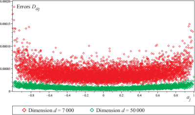
Figure 6: The time-averaged quadratic error $\tensor{*}[]{D}{{}_{a_{j}}}$ only marginally depends on the eigenstate $\rho_{0}=\ket{a_{j}}\bra{a_{j}}$, which serves as the initial state. Furthermore the deviations from the reference-function in the larger system $d=50000$ are significantly smaller than the corresponding deviations for $d=7000$.

Fig. 6 shows the averaged deviations of the expectation-value dynamics from the reference function for all eigen-states of $A$. The errors appear to be only marginally dependent on the position in the spectrum of $A$.

Fig. 6 furthermore indicates that the deviations from the reference-function decrease for larger dimension $d$. To address the dependence of the errors on the system size $d$ we plot the averaged errors $\tensor{*}[]{D}{{}_{d}}$ as a function of the reciprocal dimension $1/d$ (Fig. 4).

This finite-size scaling indicates that the mean quadratic error $\tensor{*}[]{D}{{}_{d}}$ is proportional $\frac{1}{d}$. This suggests that the variances of the errors $\tensor{*}[]{D}{{}_{a_{j}}^{t}}$ each are proportional to $\frac{1}{d}$.

Thus the properties of the error distribution are in accord with the assumptions made in (36), which in turn implies the $\frac{1}{d^{2}}$-error scaling for $N\ll d$ found in (38).

Appendix F Typicality

In this Section a derivation of Eq. (12) is presented. It is similar to a comparable analysis in Ref. Reimann and Gemmer (2019b). Consider a ensemble of pure states given by

$$\ket{\psi}=\bra{\phi}\ket{\phi}^{-1/2}\ket{\phi},\quad\ket{\phi}=\sqrt{r(A)}\ket{\xi}$$ (42)

where $r(A)$ is a nonnegative, “smooth” function, i.e., $|r(a_{j+1})-r(a_{j})|/|a_{j+1}-a_{j}|<d$, with respective expectation values $\bra{\psi}A(t)\ket{\psi}$

$$\bra{\psi}A(t)\ket{\psi}=\frac{\bra{\xi}\sqrt{r(A)}A(t)\sqrt{r(A)}\ket{\xi}}{\bra{\xi}r(A)\ket{\xi}}.$$ (43)

We analyze the statistical properties of the numerator first. Let the overbar $\overline{\cdots}$ indicate the average over all $\ket{\xi}$ and $\sigma^{2}(\cdots)$ the respective variance. Following Lloyd (2013); Gemmer et al. (2009) we obtain:

$$\overline{\bra{\xi}\sqrt{r(A)}A(t)\sqrt{r(A)}\ket{\xi}}=\mathbb{E}[r(A)A(t)],$$ (44)

$$\sigma^{2}(\bra{\xi}\sqrt{r(A)}A(t)\sqrt{r(A)}\ket{\xi})=$$ (45)

$$\frac{\chi^{2}[\sqrt{r(A)}A(t)\sqrt{r(A)}]}{d+1}\leq\frac{\mathbb{E}[r(A)A^{2}]}{d+1}$$ (46)

where $\mathbb{E}[\cdots]$ denotes the mean and $\chi^{2}[\cdots]$ the variance of the spectrum of the respective operator. As $\mathbb{E}[r(A)A^{2}]$ converges against a fixed value for large $d$ and smooth $r(A)$, the variance $\sigma^{2}(\bra{\xi}\sqrt{r(A)}A(t)\sqrt{r(A)}\ket{\xi})$ has an upper bound that essentially scales as $d^{-1}$. Hence

$$\bra{\xi}\sqrt{r(A)}A(t)\sqrt{r(A)}\ket{\xi}\approx\mathbb{E}[r(A)A(t)]=\frac{\Tr{r(A)A(t)}}{d}$$ (47)

is a very good approximation for all $\ket{\xi}$ except for a fraction of size of at most $\propto d^{-1/2}$. We now perform an analogous analysis for the denominator of Eq. (43):

$$\overline{\bra{\xi}r(A)\ket{\xi}}=\mathbb{E}[r(A)],\quad\sigma^{2}(\bra{\xi}f(A)\ket{\xi})=\frac{\chi^{2}[r(A)]}{(d+1)}$$ (48)

As $\chi^{2}[r(A)]$ converges against a fixed value for large $d$ and smooth $r(A)$, the variance $\sigma^{2}(\bra{\xi}f(A)\ket{\xi})$ essentially scales as $d^{-1}$. Hence

$$\bra{\xi}r(A)\ket{\xi}\approx\mathbb{E}[r(A)]=\frac{\Tr{r(A)}}{d}$$ (49)

is a very good approximation for all $\ket{\xi}$ except for a fraction of size of $\propto d^{-1/2}$. Inserting Eq. (47) and Eq. (49) into Eq. (43) yields

$$\bra{\psi}A(t)\ket{\psi}\approx\frac{\Tr{r(A)A(t)}}{\Tr{r(A)}}$$ (50)

as a good approximation for all $\ket{\psi}$ except for a fraction of size of at most $\propto d^{-1/2}$. This establishes Eq. (12).

References

- Gogolin and Eisert (2016) Christian Gogolin and Jens Eisert, “Equilibration, thermalisation, and the emergence of statistical mechanics in closed quantum systems,” Reports on Progress in Physics 79, 056001 (2016).
- Reimann (2008) Peter Reimann, “Foundation of statistical mechanics under experimentally realistic conditions,” Phys. Rev. Lett. 101, 190403 (2008).
- Short and Farrelly (2012) Anthony J Short and Terence C Farrelly, “Quantum equilibration in finite time,” New Journal of Physics 14, 013063 (2012).
- Linden et al. (2009) Noah Linden, Sandu Popescu, Anthony J. Short, and Andreas Winter, “Quantum mechanical evolution towards thermal equilibrium,” Phys. Rev. E 79, 061103 (2009).
- Srednicki (1994) Mark Srednicki, “Chaos and quantum thermalization,” Phys. Rev. E 50, 888–901 (1994).
- Deutsch (1991) J. M. Deutsch, “Quantum statistical mechanics in a closed system,” Phys. Rev. A 43, 2046–2049 (1991).
- Lloyd (2013) Seth Lloyd, “Pure state quantum statistical mechanics and black holes,” arXiv e-prints , arXiv:1307.0378 (2013), arXiv:1307.0378 [quant-ph] .
- Reimann (2007) Peter Reimann, “Typicality for generalized microcanonical ensembles,” Phys. Rev. Lett. 99, 160404 (2007).
- Reimann and Gemmer (2019a) Peter Reimann and Jochen Gemmer, “Full expectation-value statistics for randomly sampled pure states in high-dimensional quantum systems,” Phys. Rev. E 99, 012126 (2019a).
- Popescu et al. (2006) Sandu Popescu, Anthony J. Short, and Andreas Winter, “Entanglement and the foundations of statistical mechanics,” Nature Physics 2, 754–758 (2006).
- Tasaki (2016) Hal Tasaki, “Typicality of thermal equilibrium and thermalization in isolated macroscopic quantum systems,” Journal of Statistical Physics 163, 937–997 (2016).
- Sugiura and Shimizu (2013) Sho Sugiura and Akira Shimizu, “Canonical thermal pure quantum state,” Phys. Rev. Lett. 111, 010401 (2013).
- Goldstein et al. (2006) Sheldon Goldstein, Joel L. Lebowitz, Roderich Tumulka, and Nino Zanghì, “Canonical typicality,” Phys. Rev. Lett. 96, 050403 (2006).
- Mazur (1969) P. Mazur, “Non-ergodicity of phase functions in certain systems,” Physica 43, 533 – 545 (1969).
- Haake (1991) Fritz Haake, “Quantum signatures of chaos,” in Quantum Coherence in Mesoscopic Systems (Springer, 1991) pp. 583–595.
- Campisi et al. (2011) Michele Campisi, Peter Hänggi, and Peter Talkner, “Colloquium: Quantum fluctuation relations: Foundations and applications,” Rev. Mod. Phys. 83, 771–791 (2011).
- Richter et al. (2019) Jonas Richter, Jochen Gemmer, and Robin Steinigeweg, “Impact of eigenstate thermalization on the route to equilibrium,” Phys. Rev. E 99, 050104 (2019).
- Srednicki (1999) Mark Srednicki, “The approach to thermal equilibrium in quantized chaotic systems,” Journal of Physics A: Mathematical and General 32, 1163 (1999).
- D’Alessio et al. (2016) Luca D’Alessio, Yariv Kafri, Anatoli Polkovnikov, and Marcos Rigol, “From quantum chaos and eigenstate thermalization to statistical mechanics and thermodynamics,” Advances in Physics 65, 239–362 (2016), https://doi.org/10.1080/00018732.2016.1198134 .
- Beugeling et al. (2015) Wouter Beugeling, Roderich Moessner, and Masudul Haque, “Off-diagonal matrix elements of local operators in many-body quantum systems,” Phys. Rev. E 91, 012144 (2015).
- Mondaini and Rigol (2017) Rubem Mondaini and Marcos Rigol, “Eigenstate thermalization in the two-dimensional transverse field ising model. ii. off-diagonal matrix elements of observables,” Phys. Rev. E 96, 012157 (2017).
- Mukerjee et al. (2006) Subroto Mukerjee, Vadim Oganesyan, and David Huse, “Statistical theory of transport by strongly interacting lattice fermions,” Phys. Rev. B 73, 035113 (2006).
- Kolovsky and Buchleitner (2004) A. R Kolovsky and A Buchleitner, “Quantum chaos in the bose-hubbard model,” Europhysics Letters (EPL) 68, 632–638 (2004).
- Parra-Murillo et al. (2014) Carlos A. Parra-Murillo, Javier Madroñero, and Sandro Wimberger, “Quantum diffusion and thermalization at resonant tunneling,” Phys. Rev. A 89, 053610 (2014).
- Torres-Herrera et al. (2016) Eduardo Jonathan Torres-Herrera, Jonathan Karp, Marco Távora, and Lea F. Santos, “Realistic many-body quantum systems vs. full random matrices: Static and dynamical properties,” Entropy 18 (2016), 10.3390/e18100359.
- Nation and Porras (2018) Charlie Nation and Diego Porras, “Off-diagonal observable elements from random matrix theory: distributions, fluctuations, and eigenstate thermalization,” New Journal of Physics 20, 103003 (2018).
- Mondaini et al. (2018) Rubem Mondaini, Krishnanand Mallayya, Lea F. Santos, and Marcos Rigol, “Comment on “systematic construction of counterexamples to the eigenstate thermalization hypothesis”,” Phys. Rev. Lett. 121, 038901 (2018).
- Hamazaki and Ueda (2019) Ryusuke Hamazaki and Masahito Ueda, “Random-matrix behavior of quantum nonintegrable many-body systems with dyson’s three symmetries,” Phys. Rev. E 99, 042116 (2019).
- Foini and Kurchan (2019) Laura Foini and Jorge Kurchan, “Eigenstate thermalization and rotational invariance in ergodic quantum systems,” arXiv e-prints , arXiv:1906.01522 (2019), arXiv:1906.01522 [cond-mat.stat-mech] .
- Fine (2009) Boris V. Fine, “Typical state of an isolated quantum system with fixed energy and unrestricted participation of eigenstates,” Phys. Rev. E 80, 051130 (2009).
- Müller et al. (2011) Markus P. Müller, David Gross, and Jens Eisert, “Concentration of measure for quantum states with a fixed expectation value,” Communications in Mathematical Physics 303, 785–824 (2011).
- Reimann and Gemmer (2019b) Peter Reimann and Jochen Gemmer, “Why are macroscopic experiments reproducible? imitating the behavior of an ensemble by single pure states,” Physica A: Statistical Mechanics and its Applications , 121840 (2019b).
- Dabelow and Reimann (2019) Lennart Dabelow and Peter Reimann, “Perturbed relaxation of quantum many-body systems,” arXiv e-prints , arXiv:1903.11881 (2019), arXiv:1903.11881 [cond-mat.stat-mech] .
- Knipschild and Gemmer (2018) Lars Knipschild and Jochen Gemmer, “Stability of quantum dynamics under constant hamiltonian perturbations,” Phys. Rev. E 98, 062103 (2018).
- Richter et al. (2019) Jonas Richter, Fengping Jin, Lars Knipschild, Hans De Raedt, Kristel Michielsen, Jochen Gemmer, and Robin Steinigeweg, “Exponential damping induced by random and realistic perturbations,” arXiv e-prints , arXiv:1906.09268 (2019), arXiv:1906.09268 [cond-mat.stat-mech] .
- Foini and Kurchan (2019) Laura Foini and Jorge Kurchan, “Eigenstate thermalization hypothesis and out of time order correlators,” Phys. Rev. E 99, 042139 (2019).
- Nickelsen and Kastner (2019) Daniel Nickelsen and Michael Kastner, “Classical lieb-robinson bound for estimating equilibration timescales of isolated quantum systems,” Phys. Rev. Lett. 122, 180602 (2019).
- Figueroa-Romero et al. (2019) Pedro Figueroa-Romero, Kavan Modi, and Felix A. Pollock, “Almost Markovian processes from closed dynamics,” Quantum 3, 136 (2019).
- Jansen et al. (2019) David Jansen, Jan Stolpp, Lev Vidmar, and Fabian Heidrich-Meisner, “Eigenstate thermalization and quantum chaos in the holstein polaron model,” Phys. Rev. B 99, 155130 (2019).
- Luitz and Bar Lev (2016) David J. Luitz and Yevgeny Bar Lev, “Anomalous thermalization in ergodic systems,” Phys. Rev. Lett. 117, 170404 (2016).
- Isserlis (1918) L. Isserlis, “On A Formula For The Product-Moment Coefficient of Any Order Of A Normal Frequency Distribution In Any Number Of Variables,” Biometrika 12, 134–139 (1918), http://oup.prod.sis.lan/biomet/article-pdf/12/1-2/134/481266/12-1-2-134.pdf .
- Gemmer et al. (2009) Jochen Gemmer, Mathias Michel, and Günter Mahler, Quantum thermodynamics: Emergence of thermodynamic behavior within composite quantum systems, Vol. 784 (Springer, 2009).