Thermoelectric Generation of Orbital Magnetization in Metals

Abstract

We propose an orbital magnetothermal effect wherein a temperature gradient generates an orbital magnetization (OM) for Bloch electrons, and we present a unified theory for electrically and thermally induced OM, valid for both metals and insulators. We reveal that there exists an intrinsic response of OM, for which the susceptibilities are completely determined by the band geometric quantities such as interband Berry connections, interband orbital moments, and the quantum metric. The theory can be readily combined with first-principles calculations to study real materials. As an example, we calculate the OM response in CrI₃ bilayers, where the intrinsic contribution dominates. The temperature scaling of intrinsic and extrinsic responses, the effect of phonon drag, and the phonon angular momentum contribution to OM are discussed.

Orbital magnetization (OM) is an important fundamental property of solids, yet its theoretical calculation is notoriously difficult, made possible only relatively recently. The main problem is that the magnetic dipole operator $\bm{r}\times\bm{v}$ is ill defined for Bloch basis, which are the eigenstates for extended periodic systems. Several approaches, such as semiclassical Xiao2005 , Wannier function Resta2005 , and thermodynamic approaches Shi2007 , have been developed to circumvent this problem, and succeeded in establishing a formula of OM for a system at equilibrium.

OM may also be produced by external driving forces, e.g., through the magnetoelectric effect Vanderbilt2010 ; Murakami2015 ; Zhong2016 . Indeed, recent experiments reported signals of pronounced OM generated by applied electric field in doped monolayer MoS₂ and twisted bilayer graphene Mak2017 ; Gordon2019 ; Lee2019 , which are essentially two-dimensional (2D) metals.

This field-generated OM has distinct symmetry requirement from the equilibrium OM. As shown in Table 1, while the equilibrium OM requires the unperturbed system to have broken time-reversal ($\mathcal{T}$) symmetry, the linear-order electrically generated OM, i.e.,

$$\Delta M_{i}=\chi_{ij}E_{j},$$ (1)

requires the inversion symmetry ($\mathcal{P}$) to be broken. Here $\chi_{ij}$ is defined to be the susceptibility tensor, and summation over repeated Cartesian indices is implied henceforth. Interestingly, one observes that if the system simultaneously breaks $\mathcal{T}$, there could exist an “intrinsic” contribution, meaning that the corresponding susceptibility $\chi^{\text{int}}$ is determined solely by the band structure of the material, independent of the scattering (which gives the extrinsic contribution with $\chi^{\text{ext}}$). Furthermore, if the combined $\mathcal{PT}$ symmetry is respected, $\Delta\bm{M}$ will only have the intrinsic contribution (see Table 1).

Despite the exciting experimental discovery and the symmetry argument of its existence, so far, we do not have a coherent theory for the electrically generated OM in metals. We stress the metallic state here, because for insulators, one may derive a theory by extending the previous approaches, but for metals, which are pertinent to many experiments, these approaches do not work. For instance, there is problem in defining localized Wannier functions in metals Vanderbilt2010 ; Resta2005 ; Moore2010 ; Lee2011 , and in the presence of current flow (indicating an out-of-equilibrium system) the thermodynamic approach Xiao2005 ; Shi2007 is not applicable. This poses an outstanding challenge in condensed matter physics.

Table 1: Symmetry requirements of the equilibrium OM and the induced OM $\Delta M$ (generated by the electric field or by temperature gradient). The last two columns indicate the temperature dependence of each contribution in $\Delta M$ in the low-$T$ and the high-$T$ regimes.

OM	$\ \ \ \ \mathcal{P}$	$\ \ \mathcal{T}$	$\ \mathcal{PT}$	low-$T$	high-$T$
equilibrium OM	✓	$\times$	$\times$
intrinsic $\Delta M$	$\times$	$\times$	✓	$\ \ \ \ \ \ \sim T$	$\ \ \ \ \ \ \sim T$
extrinsic $\Delta M$	$\times$	✓	$\times$	$\ \ \ \ \ \ \sim T$	$\ \ \ \ \ \ \sim T^{0}$

Meanwhile, the temperature gradient $\nabla T$ shares the same symmetry as the $\bm{E}$ field, hence, from the symmetry perspective, there should also exist OM generated by $\nabla T$,

$$\Delta M_{i}=\alpha_{ij}(-\partial_{j}T),$$ (2)

with the same characters as in Table 1. Such an effect, which may be termed as the orbital magnetothermal effect, has not been explored before. For this effect, besides the problems in treating the OM in metals, there is additional complication in dealing with $\nabla T$: as a statistical force, it does not directly enter into the single-particle Hamiltonian as a perturbation.

In this work, we predict the orbital magnetothermal effect, and we present a unified theory for the thermally and electrically generated OM in 2D systems, applicable for both metals and insulators. We show that the induced OM can be extracted from the magnetization current, which in turn can be derived from a semiclassical theory integrating the recently developed field variational Dong2020 and second-order wave packet Gao2014 methods. Particularly, we obtain elegant formulas for the intrinsic response coefficients $\chi^{\text{int}}$ and $\alpha^{\text{int}}$, expressed by band geometric quantities such as interband Berry connections, interband orbital moments, and the quantum metric. Intriguingly, we find that $\chi^{\text{int}}$ and $\alpha^{\text{int}}$ fulfill the generalized Mott relation, thus measuring one allows us to also extract the other. Our theory can be readily combined with first-principles density-functional-theory (DFT) calculations to study real materials. As an example, we calculate the OM response in CrI₃ bilayers, where the intrinsic contribution dominates due to the $\mathcal{PT}$ symmetry.

Approach. The starting point of our approach is the intrinsic connection between OM $\bm{M}$ and the local current density $\bm{j}$. It is well known in electromagnetism that $\bm{j}$ of a nonuniform steady state consists of two parts: the transport current and the magnetization current:

$$\boldsymbol{j}=\boldsymbol{j}^{\text{tr}}+\boldsymbol{j}^{\text{mag}},\text{ \ \ }\boldsymbol{j}^{\text{mag}}=\nabla\times\bm{M}\mathbf{.}$$ (3)

The magnetization current $\bm{j}^{\text{mag}}$ does not contribute to the net current flow through a sample Cooper1997 , thus what one measures in transport experiment is $\bm{j}^{\text{tr}}$. Here, the key observation is that for 2D systems, OM is a pseudoscalar, as $\bm{M}$ only has the out-of-plane ($z$) component. Consequently, the OM can be completely determined from $\bm{j}^{\text{mag}}$ through the second equation of (3) note-uncertainty . Thus, the task can be reduced to identifying $\bm{j}^{\text{mag}}$ in the local current $\bm{j}$.

There are still three obstacles for this task. First, we need an unambiguous separation of $\bm{j}^{\text{mag}}$ from $\bm{j}^{\text{tr}}$ in $\bm{j}$. This is nontrivial, because terms in $\bm{j}^{\text{tr}}$ may also involve spatial derivatives (like $\partial_{i}T$). Fortunately, this difficulty is solved in our recent work, by the trick of a fictitious inhomogeneous field implemented in the semiclassical theory. The inhomogeneous field, assumed to be a vector, $\bm{w}(\bm{r})$, gives a spatial dependence of the electron wave packet state and energy, which helps to distinguish the $\bm{j}^{\text{mag}}$ contribution. The specific form of $\bm{w}$ does not matter, and it is set to zero at the end of the calculation. In Xiao2020EM , this method has successfully reproduced the formulas for the equilibrium OM.

Second, since we are looking for the induced OM $\Delta\bm{M}$ which is of linear order in the perturbation, $\bm{j}^{\text{mag}}$ must be evaluated to the second order (one order is from the spatial derivative of $\bm{w}$). This means that, to calculate the current we must employ a semiclassical theory with second order accuracy. Fortunately, such a framework is developed in our recent work Gao2014 and has found successful applications in various nonlinear effects Gao2015 ; Gao2017 .

Third, after clarifying the above two points, calculating the electric-field induced OM becomes straightforward. However, we still need a way to incorporate the statistical forces (such as $\nabla T$ and $\nabla\mu$, with $\mu$ the chemical potential). This is achieved by generalizing the recently developed field variational approach Dong2020 to incorporate the second-order semiclassical dynamics, which gives a unified treatment of both electric field and statistical forces.

In the Supplemental Material supp , we present detailed derivations based on the wave packet action $S$, where the local current can be formally expressed as (set $\hbar=1$)

$$\boldsymbol{j}\left(\boldsymbol{r}\right)=\int\left[d\boldsymbol{k}_{c}\right]d\boldsymbol{r}_{c}\mathcal{D}f_{\text{tot}}\frac{\delta S}{\delta\boldsymbol{A}\left(\boldsymbol{r}\right)}\Big{|}_{\boldsymbol{A}\left(\boldsymbol{r}\right)\rightarrow 0}.$$ (4)

Here, $(\bm{r}_{c},\bm{k}_{c})$ are the center of the electron wave packet in phase space, $\left[d\boldsymbol{k}_{c}\right]\equiv\sum_{n}d\boldsymbol{k}_{c}/\left(2\pi\right)^{2}$ with $n$ the band index, $\mathcal{D}$ is the modified phase space measure Xiao2010 , $f_{\text{tot}}$ is the occupation function, and $\bm{A}$ is the vector potential, an auxiliary field which is set to zero at the end of the derivation.

Taking into account the fictitious inhomogeneous field, the variation yields (the subscripts $c$ are dropped hereafter and we omit the band index here)

$$\boldsymbol{j}=e\int\left[d\boldsymbol{k}\right]\mathcal{D}f_{\text{tot}}\boldsymbol{\dot{r}}+\boldsymbol{\nabla}\times\int\left[d\boldsymbol{k}\right]\mathcal{D}f_{\text{tot}}(\boldsymbol{\tilde{m}}+\dot{k}_{j}\partial_{\bm{B}}a_{j}^{B}),$$ (5)

where $(\dot{\bm{r}},\dot{\bm{k}})$ are given by the second-order equations of motion

$$\dot{\boldsymbol{r}}= \ \partial_{\boldsymbol{k}}\tilde{\varepsilon}-\dot{\boldsymbol{k}}\times\mathbf{\tilde{\Omega}}-\mathbf{\tilde{\Omega}}_{\boldsymbol{kr}}\cdot\dot{\boldsymbol{r}},$$

$$\dot{\boldsymbol{k}}= \ e\boldsymbol{E}-\partial_{\boldsymbol{r}}\tilde{\varepsilon}+\mathbf{\tilde{\Omega}}_{\boldsymbol{rk}}\cdot\dot{\boldsymbol{k}}.$$ (6)

Here, $e(<0)$ is the electron charge, $\boldsymbol{\tilde{m}}$ is the orbital magnetic moment, $\tilde{\varepsilon}$ is the wave packet energy, $\mathbf{\tilde{\Omega}}$ is the momentum space Berry curvature, $\mathbf{\tilde{\Omega}}_{\boldsymbol{kr}}=-\mathbf{\tilde{\Omega}}_{\boldsymbol{rk}}$ is the phase space Berry curvature, and $\mathcal{D}=1+\text{Tr}\,\mathbf{\tilde{\Omega}}_{\boldsymbol{kr}}$. The tilde in these symbols indicates that they include corrections from the external fields. The detailed expressions for these quantities do not concern us here, and can be found in the Supplemental Material supp . $\bm{a}^{B}$ is known as the field-induced positional shift Gao2014 , representing the linear correction to the $\boldsymbol{k}$-space Berry connection by the magnetic field $\bm{B}$, hence the term $\partial_{\bm{B}}a_{j}^{B}$ in (5) is independent of $\bm{B}$. The importance of this term to the induced OM will be shown shortly.

We make the following observations on the result in Eq. (5). First, to distinguish intrinsic and extrinsic contributions, we write $f_{\text{tot}}=f_{0}+\delta f$ in (5), with $f_{0}$ the equilibrium Fermi distribution and $\delta f$ the off-equilibrium part. Then, the intrinsic contribution of the induced OM $\Delta\bm{M}^{\text{int}}$ will contain terms with only $f_{0}$, whereas the extrinsic contribution will contain $\delta f$ and hence depend on the scattering processes (manifested, e.g., by the carrier relaxation time). Clearly, $\Delta\bm{M}^{\text{int}}$ is of more interest, so below we will focus on the intrinsic contribution. The extrinsic contribution is analyzed in Refs. Murakami2015 ; Zhong2016 , and its typical behavior will be commented later.

Second, to account for $\Delta\bm{M}$ in the linear order of the driving forces, it is sufficient to take $\mathcal{D}=1$ in the second term on the right hand side of (5), so that the contribution of this term to $\Delta\bm{M}^{\text{int}}$ is ($\partial_{j}\equiv\partial/\partial r_{j}$ henceforth) $\boldsymbol{\nabla}\times\int\left[d\boldsymbol{k}\right]f_{0}[\boldsymbol{\tilde{m}}+(eE_{j}-\partial_{j}\varepsilon)\partial_{\bm{B}}a_{j}^{B}]$.

Third, comparing the form of Eq. (5) to Eq. (3), one might be tempted to identify the second term on the right hand side of (5) as $\bm{j}^{\text{mag}}$. However, this is incorrect for $\Delta\bm{M}^{\text{int}}$. Similar to Refs. Xiao2020EM ; Dong2020 , by tracing the $\bm{w}$ field, one finds that the first term in (5) actually also contains a part that belongs to $\bm{j}^{\text{mag}}$. Detailed calculations supp show that the sum of this part and the $\boldsymbol{\tilde{m}}$ term in Eq. (5) gives the equilibrium OM.

Finally, according to the above observations, the quantity $(eE_{j}-\partial_{j}\varepsilon)f_{0}\partial_{\bm{B}}a_{j}^{B}$ plays the decisive role in $\Delta\bm{M}^{\text{int}}$. The statistical forces naturally enter into the picture through the factor $f_{0}\partial_{j}\varepsilon=\partial_{j}g_{0}-\partial_{T}g_{0}\partial_{j}T-\partial_{\mu}g_{0}\partial_{j}\mu$, where $g_{0}=-\int_{\varepsilon}^{\infty}d\eta f_{0}(\eta)$.

Intrinsic orbital magnetoelectric and magnetothermal effects. Combining these considerations and collecting terms that are linear in the driving forces of $\bm{E}$, $\nabla T$, and $\nabla\mu$, we arrive at the following result for the intrinsic field-generated OM:

$$\Delta M^{\text{int}}=\boldsymbol{\chi}^{\text{int}}\cdot(\boldsymbol{E}-{\nabla}\mu/e)-\boldsymbol{\alpha}^{\text{int}}\cdot{\nabla}T,$$ (7)

where we have used the fact that for 2D, OM only has the $z$-component (with $\Delta\bm{M}^{\text{int}}=\Delta M^{\text{int}}\hat{z}$), and hence it is convenient to also express the susceptibility tensors in vector forms, given by

$$\boldsymbol{\chi}^{\text{int}}=e\int\left[d\boldsymbol{k}\right]f_{0}\bm{\Lambda}^{n},$$ (8)

$$\boldsymbol{\alpha}^{\text{int}}=\int\left[d\boldsymbol{k}\right]s_{0}\bm{\Lambda}^{n},$$ (9)

with

$$s_{0}=\left(\varepsilon-\mu\right)f_{0}/T+k_{B}\ln[1+e^{-(\varepsilon-\mu)/k_{B}T}]$$ (10)

being the entropy density contributed by a particular state. The common factor $\bm{\Lambda}^{n}$ in Eqs. (8) and (9) is given by (we restore $\hbar$ and band indices $n$, $m$ here)

$$\Lambda_{i}^{n}=2\operatorname{Re}\sum_{m\neq n}\frac{\mathcal{A}_{i}^{nm}\mathcal{M}^{mn}}{\varepsilon_{n}-\varepsilon_{m}}+\frac{e}{2\hbar}\epsilon_{j\ell}\partial_{k_{j}}\mathcal{G}_{i\ell}^{n},$$ (11)

where $\bm{\mathcal{A}}^{nm}=\langle u_{n}|i\partial_{\bm{k}}|u_{m}\rangle$ is the interband Berry connection, $\mathcal{M}^{mn}=(e/2)\sum_{m^{\prime}\neq n}[(\boldsymbol{v}^{mm^{\prime}}+\boldsymbol{v}^{n}\delta_{mm^{\prime}})\times\bm{\mathcal{A}}^{m^{\prime}n}]_{z}$ is the interband orbital magnetic moment with $\boldsymbol{v}^{mm^{\prime}}$ being the velocity matrix element, $\mathcal{G}_{i\ell}^{n}=\operatorname{Re}\langle\partial_{k_{i}}u_{n}|\partial_{k_{\ell}}u_{n}\rangle-\bm{\mathcal{A}}_{i}^{n}\bm{\mathcal{A}}_{\ell}^{n}$ is the Fubini-Study quantum metric for band $n$ QM2020 ; QM1980 , and $\epsilon_{ij}$ is the 2D Levi-Civita symbol. Equations (7)-(11) are the key results of this work. They present for the first time a unified theory for the electrically and thermally generated OM, applicable for both metals and insulators.

The result exhibits several nice features. First, the first term on the right hand side of Eq. (7) explicitly shows that the Einstein relation, i.e., the equivalence between $\bm{E}$ field and chemical potential gradient, is fulfilled in our theory. It has to be stressed that this fulfillment is quite nontrivial: the $\bm{E}$ field enters through the equations of motion (6) as well as the field corrections in the quantities in Eq. (5), whereas $\nabla\mu$ enters only through the occupation function. Therefore, the consistency with the Einstein relation serves as a nice check for the validity of our theory.

Second, the two susceptibilities $\bm{\chi}^{\text{int}}$ and $\bm{\alpha}^{\text{int}}$, representing magnetoelectric and magnetothermal responses, satisfy the generalized Mott relation

$$\boldsymbol{\alpha}^{\text{int}}=\int d\eta\ \partial_{\eta}f_{0}\frac{\eta-\mu}{eT}\boldsymbol{\chi}^{\text{int}}\left(\eta\right),$$ (12)

where $\boldsymbol{\chi}^{\text{int}}\left(\eta\right)$ is the value of (8) at zero temperature, taken to be a function of the chemical potential $\eta$. At low temperatures, the above equation reduces to

$$\boldsymbol{\alpha}^{\text{int}}=\frac{\pi^{2}k_{B}^{2}T}{3e}\partial_{\eta}\boldsymbol{\chi}^{\text{int}}\left(\eta\right)|_{\eta=\mu}.$$ (13)

Traditionally, the Mott relation is between the electric and thermal conductivities. Recent works have extended its applicability to various Berry curvature related linear responses, such as spin polarization and spin torques Freimuth2014 ; Shitade2019 ; Dong2020 . Here, we have shown that it also establishes a connection between orbital magnetoelectric and magnetothermal effects.

Third, as promised, the intrinsic susceptibilities $\bm{\chi}^{\text{int}}$ and $\bm{\alpha}^{\text{int}}$ comprise only band geometric quantities. Interestingly, the Berry curvature does not appear in (11), instead, there emerges the quantum metric. Geometrically, the quantum metric measures the distance between neighboring Bloch states. It has attracted great interest, because of its appearance in various nonlinear effects discovered in recent works QM2020 ; Lapa2019 ; Gao2015 . Note that all quantities in (11) are gauge invariant, which makes it convenient to be combined with first-principles calculations for real materials.

Application to bilayer CrI₃. We demonstrate the application of our theory in studying a real material. It is important to note that crystalline symmetries also impose constraints on these effects. From Eq. (7), we see that the susceptibilities behave as in-plane pseudo-vectors (the same symmetry as the Berry curvature dipole Fu2015 ). Thus, the largest spatial symmetry allowed in 2D is a single mirror line. Guided by this constraint, we consider the example of bilayer CrI₃.

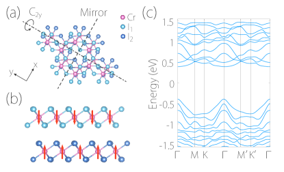
Figure 1: (a) Top and (b) side view of the structure of CrI₃ bilayer. Green (blue) balls represent I atoms in the top (bottom) layer. The arrows depict the local spin orientation. (c) Calculated band structure of CrI₃ bilayer.

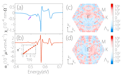
Figure 2: Calculated susceptibilities (a) $\chi_{x}$ and (b) $\alpha_{x}$ versus the chemical potential for CrI₃ bilayer. The inset in (b) shows the temperature dependence of $\alpha_{x}$ at 0.5 eV. (c) and (d) show the momentum space distribution of $\Lambda_{x}(\boldsymbol{k})$ and $\Lambda_{y}(\boldsymbol{k})$ at 0.5 eV (marked by the arrow in (a)), in the unit of $e\hbar^{-1}\cdot\text{\AA}^{-3}$. In the calculation, we take $T=10$ K.

CrI₃ is a van der Waals layered magnetic material. Monolayer and bilayer CrI₃ have been successfully fabricated in experiment. The bilayer CrI₃ has a monoclinic ($C2/m$) crystal structure Sun2019 , and it was demonstrated to be a 2D antiferromagnet at ground state Huang2017 ; Seyler2018 . As shown in Figs. 1(a) and (b), the magnetic moments are mainly on the Cr sites. The coupling within each layer is ferromagnetic, whereas the interlayer coupling is of antiferromagnetic type. Clearly, both $\mathcal{P}$ and $\mathcal{T}$ are broken in this system, therefore the intrinsic orbital magnetoelectric and magnetothermal effects are allowed. Furthermore, the configuration preserves the $\mathcal{PT}$ symmetry, under which the intrinsic contribution will be the dominant OM response (the equilibrium OM also vanishes, see Table 1).

The susceptibilities $\bm{\chi}^{\text{int}}$ and $\bm{\alpha}^{\text{int}}$ have been evaluated by our theory combined with DFT calculations (see Supplemental Material supp for details). Figure 1(c) shows the band structure of bilayer CrI₃ obtained from DFT calculations. Note that the system has a twofold rotational axis $c_{2y}$ (see Fig. 1(a)), which requires $\bm{\chi}^{\text{int}}$ and $\bm{\alpha}^{\text{int}}$ to be along the $x$ direction. This feature is confirmed by our DFT calculation. In Fig. 2, we plot the values of the two susceptibilities as functions of the chemical potential, which can physically be tuned by gating (for simplicity, we fix the magnetic configuration in the calculation, which in reality may be achieved by pinning with neighboring magnetic layers). One observes that both $\bm{\chi}^{\text{int}}$ and $\bm{\alpha}^{\text{int}}$ are very small inside the band gap. However, they increase rapidly under doping. $\chi^{\text{int}}$ can reach a typical magnitude of $10^{-4}$ nm/$\Omega$. Assuming an applied $E$ field of $10^{4}$ V/m (along $x$), the induced magnetization, which is out-of-plane, can reach $\sim 10^{-4}\mu_{B}/\text{nm}^{2}$, which is two orders larger than that observed in doped monolayer MoS₂ Mak2017 , and is of the same order as the Edelstein effect in strongly Rashba spin-orbit-coupled materials such as the Au(111) surface Johansson2016 .

The Mott relation in (13) indicates a linear temperature scaling for $\alpha^{\text{int}}$ at low $T$ regime. This behavior is also explicitly demonstrated by our calculation, as shown in the inset of Fig. 2(b). In addition, in Figs. 2(c) and (d), we plot the $\bm{k}$-resolved $x$ and $y$ components of $\bm{\Lambda}(\bm{k})=\sum_{n}f(\varepsilon_{n})\bm{\Lambda}^{n}(\bm{k})$, defined for all occupied states. One observes that governed by the $c_{2y}$ symmetry, $\Lambda_{x}$ ($\Lambda_{y}$) is an even (odd) function with respect to the $y$ axis. It follows that only the $x$ component survives after the integration over the Brillouin zone.

Discussion. In this work, we have predicted a new effect—the orbital magnetothermal effect, and we have developed a unified theory for both orbital magnetoelectric and magnetothermal effects. In the main text, we have focused on the intrinsic contribution, which is solely determined by the band structure properties, regardless of the carrier scattering. In general, extrinsic contribution would also exist. For instance, when $\mathcal{P}$, $\mathcal{T}$ and $\mathcal{PT}$ are all broken, the extrinsic and intrinsic OM responses may compete with each other. Nevertheless, we can distinguish them by their different scaling behavior. We find that when elastic or quasi-elastic scattering dominates, the extrinsic contributions also comply with the Mott relation $\boldsymbol{\alpha}^{\text{ext}}=\frac{\pi^{2}k_{B}^{2}T}{3e}\partial_{\eta}\boldsymbol{\chi}^{\text{ext}}\left(\eta\right)|_{\eta=\mu}$. In the high-$T$ regime, the electron-phonon scattering dominates, we have $\boldsymbol{\alpha}^{\text{ext}}\sim T^{0}$ due to the $T^{-1}$ scaling of the electron-phonon relaxation time $\tau_{ep}$ Ziman1972 . At low temperatures, the electron-impurity scattering dominates, then $\boldsymbol{\alpha}^{\text{ext}}\sim T$, due to the $T$ independence of the electron-impurity relaxation time $\tau_{i}$.

A temperature gradient can induce an off-equilibrium phonon distribution, which in turn drives electrons out of equilibrium through the electron-phonon coupling and hence may generate an additional extrinsic contribution, the phonon-drag OM. The pertinent correction to the electronic occupation has the form of $\delta f^{\text{g}}\propto(\tau_{i}\tau_{p}/\tau_{ep})(\nabla T/T)$ in the relaxation time approximation, where $\tau_{p}$ is the phonon relaxation time. At low temperatures, $\tau_{p}$ is a constant, limited by the boundary scattering Lyo1988 , and $\tau_{ep}^{-1}$ usually takes the form of a power-law, e.g., $T^{4}$ in a MoS₂ monolayer Jauho2013 . The phonon-drag OM thus increases with $T$ until the phonon-phonon scattering degrades $\tau_{p}$ significantly. Therefore, a peak in its $T$ dependence is anticipated, similar to the well-confirmed peak in the phonon-drag thermopower Lei2010 .

Finally, we mention that in doped ionic materials with reduced symmetry, under a temperature gradient, the off-equilibrium phonons carrying angular momentum Zhang2014 ; Spaldin2019 may also produce an induced OM Murakami2018 . Being proportional to $\tau_{p}$, this contribution is expected to be strongly suppressed at high temperatures, where the electron contribution prevails. Besides, it scales as $T^{2}$ at low temperatures in 2D Murakami2020 , which is also sub-dominant compared to the electron contribution $\sim T$. This qualitative analysis suggests that the electron OM is likely to be dominating in a wide temperature regime.

- (1) D. Xiao, J. Shi, and Q. Niu, Phys. Rev. Lett. 95, 137204 (2005).
- (2) T. Thonhauser, D. Ceresoli, D. Vanderbilt, and R. Resta, Phys. Rev. Lett. 95, 137205 (2005).
- (3) J. Shi, G. Vignale, D. Xiao, and Q. Niu, Phys. Rev. Lett. 99, 197202 (2007).
- (4) A. Malashevich, I. Souza, S. Coh, and D. Vanderbilt, New J. Phys. 12, 053032 (2010).
- (5) T. Yoda, T. Yokoyama, and S. Murakami, Sci. Rep. 5, 12024 (2015).
- (6) S. Zhong, J. E. Moore, and I. Souza, Phys. Rev. Lett. 116, 077201 (2016).
- (7) J. Lee, Z. Wang, H. Xie, K. F. Mak, and J. Shan, Nat. Mater. 16, 887 (2017).
- (8) J. Son, K.-H. Kim, Y. H. Ahn, H.-W. Lee, and J. Lee, Phys. Rev. Lett. 123, 036806 (2019).
- (9) A. L. Sharpe, E. J. Fox, A. W. Barnard, J. Finney, K. Watanabe, T. Taniguchi, M. A. Kastner, and D. Goldhaber-Gordon, Science 365, 605 (2019); W.-Y. He, D. Goldhaber-Gordon, and K. T. Law, Nat. Commun. 11, 1650 (2020).
- (10) A. M. Essin, A. M. Turner, J. E. Moore, and D. Vanderbilt, Phys. Rev. B 81, 205104 (2010).
- (11) K.-T. Chen and P. A. Lee, Phys. Rev. B 84, 205137 (2011).
- (12) L. Dong, C. Xiao, B. Xiong, and Q. Niu, Phys. Rev. Lett. 124, 066601 (2020).
- (13) Y. Gao, S. A. Yang, and Q. Niu, Phys. Rev. Lett. 112, 166601 (2014).
- (14) N. R. Cooper, B. I. Halperin, and I. M. Ruzin, Phys. Rev. B 55, 2344 (1997).
- (15) From Eq. (3), OM can only be determined up to a gradient in 3D (there is not such an uncertainty in 2D). In equilibrium, OM could be a well behaved bulk property. However, under field, the definition must involve the electric polarization, which is ill defined in metals. For 3D metals, it is currently unknown whether the field-induced OM can be well defined.
- (16) C. Xiao and Q. Niu, Phys. Rev. B 101, 235430 (2020).
- (17) Y. Gao, S. A. Yang, and Q. Niu, Phys. Rev. B 91, 214405 (2015).
- (18) Y. Gao, S. A. Yang, and Q. Niu, Phys. Rev. B 95, 165135 (2017); Y. Gao, Frontiers of Physics 14, 33404 (2019); B. Xiong, Ph.D. dissertation, The University of Texas, Austin, 2019.
- (19) See Supplementary Material for the detailed derivation of our theory.
- (20) D. Xiao, M.-C. Chang, and Q. Niu, Rev. Mod. Phys. 82, 1959 (2010).
- (21) J. P. Provost and G. Vallee, Commun. Math. Phys. 76, 289 (1980).
- (22) A. Gianfrate, O. Bleu, L. Dominici, V. Ardizzone, M. De Giorgi, D. Ballarini, G. Lerario, K. W. West, L. N. Pfeiffer, D. D. Solnyshkov, D. Sanvitto, and G. Malpuech, Nature 578, 381 (2020).
- (23) F. Freimuth, S. Blugel, and Y. Mokrousov, J. Phys.: Condens. Matter 26, 104202 (2014).
- (24) A. Shitade, A. Daido, and Y. Yanase, Phys. Rev. B 99, 024404 (2019).
- (25) M. F. Lapa, and T. L. Hughes, Phys. Rev. B 99, 121111(R) (2019).
- (26) I. Sodemann and L. Fu, Phys. Rev. Lett. 115, 216806 (2015).
- (27) Z. Sun, Y. Yi, T. Song, G. Clark, B. Huang, Y. Shan, S. Wu, D. Huang, C. Gao, Z. Chen, M. McGuire, T. Cao, D. Xiao, W.-T. Liu, W. Yao, X. Xu and S. Wu, Nature 572, 497-501 (2019).
- (28) B. Huang, G. Clark, E. Navarro-Moratalla, D. R. Klein, R. Cheng, K. L. Seyler, D. Zhong, E. Schmidgall, M. A. McGuire, D. H. Cobden, W. Yao, D. Xiao, P. Jarillo-Herrero and X. Xu, Nature 546, 270-273 (2017).
- (29) K. L. Seyler, D. Zhong, D. R. Klein, S. Gao, X. Zhang, B. Huang, E. Navarro-Moratalla, L. Yang, D. H. Cobden, M. A. McGuire, W. Yao, D. Xiao, P. Jarillo-Herrero, and X. Xu, Nat. Phys. 14, 277-281 (2018).
- (30) A. Johansson, J. Henk, and I. Mertig, Phys. Rev. B 93, 195440 (2016).
- (31) J. M. Ziman, Principles of the Theory of Solids (Cambridge University Press, Cambridge, 1972).
- (32) S. K. Lyo, Phys. Rev. B 38, 6345 (1988).
- (33) K. Kaasbjerg, K. S. Thygesen, and A.-P. Jauho, Phys. Rev. B 87, 235312 (2013).
- (34) W. S. Bao, S. Y. Liu and X. L. Lei, J. Phys.: Condens. Matter 22, 315502 (2010), and references therein.
- (35) L. Zhang and Q. Niu, Phys. Rev. Lett. 112, 085503 (2014); Phys. Rev. Lett. 115, 115502 (2015).
- (36) D. M. Juraschek and N. A. Spaldin, Phys. Rev. Mater. 3, 064405 (2019).
- (37) M. Hamada, E. Minamitani, M. Hirayama, and S. Murakami, Phys. Rev. Lett. 121, 175301 (2018).
- (38) M. Hamada and S. Murakami, Phys. Rev. B 101, 144306 (2020).