Simplifying Activity-on-Edge Graphs

Abstract

We formalize the simplification of activity-on-edge graphs used for visualizing project schedules, where the vertices of the graphs represent project milestones, and the edges represent either tasks of the project or timing constraints between milestones. In this framework, a timeline of the project can be constructed as a leveled drawing of the graph, where the levels of the vertices represent the time at which each milestone is scheduled to happen. We focus on the following problem: given an activity-on-edge graph representing a project, find an equivalent activity-on-edge graph—one with the same critical paths—that has the minimum possible number of milestone vertices among all equivalent activity-on-edge graphs. We provide a polynomial-time algorithm for solving this graph minimization problem.

1 Introduction

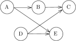
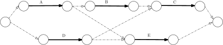
Figure 1: An activity-on-node graph, above, and its naively expanded activity-on-edge graph, below, with solid arrows as task edges and dashed-dotted arrows as unlabeled edges.

The critical path method is used in project modeling to describe the tasks of a project, along with the dependencies among the tasks; it was originally developed as PERT by the United States Navy in the 1950s [malcolm1959application]. A dependency graph is used to identify bottlenecks, and in particular to find the longest path among a sequence of tasks, where each task has a required length of time to complete (this is known as the critical path).

In this paper we are interested in the problem of visualizing an abstract timeline of the possible critical paths of a given project, represented abstractly as a partially ordered set of tasks, at a point in the project planning at which we do not yet know the time lengths of each task. The most common method of visualizing partially ordered sets, as an activity-on-node graph (a transitively reduced directed acyclic graph with a vertex for each task) is unsuitable for this aim, because it represents each task as a point instead of an object that can extend over a span of time in a timeline. To resolve this issue, we choose to represent each task as an edge in a directed acyclic graph. In this framework, the endpoints of the task edges have a natural interpretation, as the milestones of the project to be scheduled. Additional unlabeled edges do not represent tasks to be performed within the project, but constrain certain pairs of milestones to occur in a certain chronological order. The resulting activity-on-edge graph can then be drawn in standard upward graph drawing style [bt1992area, battista1998graph, gt2001computational, gt1995upward, ahr2010improving]. Alternatively, once the lengths of the tasks are known and the project has been scheduled, this graph can be drawn in leveled style [junger1999level, hkl2004characterization], where the level of each milestone vertex represents the time at which it is scheduled.

It is straightforward to expand an activity-on-node graph into an activity-on-edge graph by expanding each task vertex of the activity-on-node graph into a pair of milestone vertices connected by a task edge, with the starting milestone of each task retaining all of the incoming unlabeled edges of the activity-on-node graph and the ending milestone retaining all of the outgoing edges. It is convenient to add two more milestones at the start and end of the project, connected respectively to all milestones with no incoming edges and from all milestones with no outgoing edges. The size of the resulting activity-on-edge graph is linear in the size of the activity-on-node graph. An example of such a transformation is depicted in Figure 1.

However, the graphs that result from this naive expansion are not minimal. Often, one can merge some pairs of milestones (for instance the ending milestone of one task and the starting milestone of another task) to produce a simpler activity-on-edge graph (such as the one for the same schedule in Figure 2). Despite having fewer milestones, this simpler graph can be equivalent to the original, in the sense that its critical paths (maximal sequences of tasks that belong to a single path in the graph) are the same. By being simpler, this merged graph should aid in the visualization of project schedules. In this paper we formulate and provide a polynomial time algorithm for the problem of optimal simplification of activity-on-edge graphs.

1.1 New Results

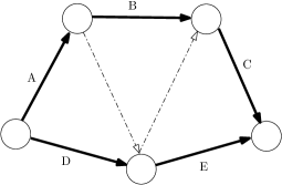
Figure 2: A simplification of the graph from Figure 1.

We describe a polynomial-time algorithm which, given an activity-on-edge graph (i.e., a directed acyclic graph with a subset of its edges labeled as tasks), produces a directed acyclic graph that preserves the critical paths of the graph and has the minimum possible number of vertices among all critical-path-preserving graphs for the given input. Our algorithm is agnostic about the weights of the tasks. In more general terms, the resulting graph has the following properties:

• The task edges in the given graph correspond one-to-one with the task edges in the new graph.

• The new graph has the same dependency (reachability) relation among task edges as the original graph.

• The new graph has the same potential critical paths as the original graph.

• The number of vertices of the graph is minimized among all graphs with the first three properties.

Our algorithm repeatedly applies a set of local reduction rules, each of which either merges a pair of adjacent vertices or removes an unlabeled edge, in arbitrary order. When no rule can be applied, the algorithm outputs the resulting graph.

We devote the rest of this section to related work and then describe the preliminaries in Section 2. We then present the algorithm in Section 3 and show in Section 4 that its output preserves the potential critical paths of the input, and in Section 5 that it has the minimum possible number of vertices. We also show that the output is independent of the order in which the rules are applied. We discuss the running time in LABEL:sec:analysis and conclude with LABEL:sec:conclusion.

1.2 Related work

Constructing clear and aesthetically pleasing drawings of directed acyclic graphs is an old and well-established task in graph drawing, with many publications [sugiyama1981methods, battista1998graph, bm2001layered, hn2014hierarchical]. The work in this line that is most closely relevant for our work involves upward drawings of unweighted directed acyclic graphs [bt1992area, gt2001computational, gt1995upward, ahr2010improving] or leveled drawings of directed acyclic graphs that have been given a level assignment [junger1999level, hkl2004characterization] (an assignment of a $y$-coordinate to each vertex, for instance representing its height on a timeline).

Although multiple prior publications use activity-on-edge graphs [kulkarni1984compact, cg1986parallel, arh1994nearcritical, hd2011project] and even consider graph drawing methods specialized for these graphs [xu2010automatic], we have been unable to locate prior work on their simplification. This problem is related to a standard computational problem, the construction of the transitive reduction of a directed acyclic graph or equivalently the covering graph of a partially ordered set [agu1972transitive]. We note in addition our prior work on augmenting partially ordered sets with additional elements (preserving the partial order on the given elements) in order to draw the augmented partial order as an upward planar graph with a minimum number of added vertices [es2013confluent].

The PERT method may additionally involve the notion of “float”, in which a given task may be delayed some amount of time (depending on the task) without any effect on the overall time of the project [arditi2006selecting, householder1990owns]. We do not consider constraints of this form in the present work, although the unlabeled edges of our output can in some sense be seen as serving a similar purpose.

2 Preliminaries

We first define an activity-on-edge graph. The graph can be a multigraph to allow tasks that can be completed in parallel to share both a start and end milestone when possible.

Definition 2.1.

Define an activity-on-edge graph (AOE) as a directed acyclic multigraph $G=(V,E)$, where a subset of the edges of $E$, denoted $\mathcal{T}$, are labeled as task edges. The labels, denoting tasks, are distinct, and we identify each edge in $\mathcal{T}$ with its label.

Definition 2.2.

Given an AOE $G$ with tasks $\mathcal{T}$, for all $T\in\mathcal{T}$, let $\operatorname{St}_{G}(T)$ be the start vertex of $T$, and let $\operatorname{End}_{G}(T)$ be the end vertex of $T$.

When the considered graph is clear from context, we omit the subscript $G$ and write $\operatorname{St}(T)$ and $\operatorname{End}(T)$. It may be that $\operatorname{St}(T)=\operatorname{St}(T^{\prime})$, or $\operatorname{End}(T)=\operatorname{End}(T^{\prime})$, or $\operatorname{End}(T)=\operatorname{St}(T^{\prime})$ with $T\neq T^{\prime}$.

To define potential critical paths formally, we introduce the following notation.

Definition 2.3.

Given an AOE $G$ with tasks $\mathcal{T}$, for all $T$, $T^{\prime}$ with $T\neq T^{\prime}$, say that $T$ has a path to $T^{\prime}$ in $G$ if there exists a path from $\operatorname{End}(T)$ to $\operatorname{St}(T^{\prime})$, or if $\operatorname{End}(T)=\operatorname{St}(T^{\prime})$, and write $T\rightsquigarrow_{G}T^{\prime}$.

Definition 2.4.

Given an AOE $G$ with tasks $\mathcal{T}$, define a potential critical path as a sequence of tasks $P=(T_{1},\dots,T_{k})$, where for all $i=1,\dots,k-1$, $T_{i}\rightsquigarrow_{G}T_{i+1}$, and where $P$ is not a subsequence of any other sequence with this property.

Our algorithm will apply a set of transformation rules to an input AOE of a canonical form.

Definition 2.5.

A canonical AOE is an AOE which is naively expanded from an activity-on-node graph.

Every AOE $G$ can be transformed into a canonical AOE with the same reachability relation on its tasks. First, we start by computing the reachability relation of the tasks. The transitive closure of the resulting reachability matrix gives an activity-on-node graph (which is quadratic, in the worst case, in the size of the original AOE). Then, this activity-on-node graph can be converted to a canonical AOE as described in Section 1.

Definition 2.6.

Two AOE graphs $G$ and $H$ are equivalent, i.e. $G\equiv H$, if $G$ and $H$ have the same set of tasks—i.e., there is a label-preserving bijection between the task edges of $G$ and those of $H$—and, with respect to this bijection, $G$ and $H$ have the same set of potential critical paths.

Definition 2.7.

An AOE $G$ is optimal if $G$ minimizes the number of vertices for its equivalence class: i.e., if for every AOE $H\equiv G$, $|V(H)|\geq|V(G)|$.

We now formally define our problem.
Problem 1. Given a canonical AOE $G$, find some optimal AOE $H$ with $H\equiv G$.

3 Simplification Rules

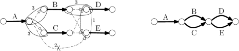
Figure 3: On the left, an AOE in which each of rules 1-3 can be applied, and on the right, the corresponding graph output by the algorithm.

Our algorithm takes a canonical AOE and greedily applies a set of rules until no more rules can be applied. Given an AOE $G=(V,E)$ and given two distinct vertices $u,v\in V$, the simplification rules used by our algorithm are:

1. if $u$ and $v$ have no outgoing task edges and have precisely the same outgoing neighbors, merge $u$ and $v$. Symmetrically, if $u$ and $v$ have no incoming task edges and have precisely the same incoming neighbors, merge $u$ and $v$.

2. If $u$ has an unlabeled edge to $v$, and $u$ has another path to $v$, remove the edge $(u,v)$.

3. If $u$ has an unlabeled edge to $v$ and the following conditions are satisfied, merge $u$ and $v$:

   • rule 2 is not applicable to the edge $(u,v)$.

   • if $u$ has an outgoing task, then $v$ has no incoming edge other than $(u,v)$.

   • if $v$ has an incoming task, then $u$ has no outgoing edge other than $(u,v)$.

   • every incoming neighbor of $v$ has a path to every outgoing neighbor of $u$.

Figure 3 depicts an AOE graph and the graph output by the algorithm after applying all possible rules.

It will be convenient for the proofs in Section 5 to give a name to the output of the algorithm:

Definition 3.1.

An output AOE, denoted

4 Correctness

In this section we prove the correctness of our algorithm (its output graph is equivalent to its input graph).

We begin with preserving potential critical paths. We show that the rules never change the existence or nonexistence of a path from one task to another, and that this implies preservation of potential critical paths.

Lemma 4.1.

Given two AOEs $G$ and $H$ with the same set of tasks $\mathcal{T}$, $G$ and $H$ have the same reachability relation $\rightsquigarrow$ on the tasks if and only if $G\equiv H$.

Proof 4.2.

Trivially, we have $T\rightsquigarrow_{G}T^{\prime}$ (or $T\rightsquigarrow_{H}T^{\prime}$) if and only if $T$ is earlier than $T^{\prime}$ in some potential critical path of $G$ (or $H$). Therefore, preservation of critical paths is equivalent to preservation of the reachability relation.

Lemma 4.3.

The output of the algorithm is equivalent to its input.

Proof 4.4.

We show the invariant that given tasks $T$ and $T^{\prime}$, $T\rightsquigarrow T^{\prime}$ at a given iteration of the algorithm if and only if $T\rightsquigarrow T^{\prime}$ at the next iteration. From this it follows that the output of the algorithm has the same reachability relation on its tasks as the input, and then the lemma follows from Lemma 4.1.

The invariant is true because merging a pair of vertices (rules 1 and 3) never disconnects a path, and no edge is ever removed (by rule 2) between two vertices unless another path exists between the two vertices. In particular, the end vertex of $T$ still has a path to the start vertex of $T^{\prime}$ after the application of any of the rules.

For the other direction, removing an edge never introduces a new path. Furthermore, if vertices $u$ and $v$ are merged by applying rule 1, and if some vertex $w$ has a path to some vertex $z$ through the newly merged $uv$, then the condition of rule 1 ensures that $w$ has a path, through $u$ or $v$, to $z$ before the merge. Similarly, suppose $u$ and $v$ are merged by applying rule 3. Then if $w$ has a path to $z$ through $uv$, then (abusing notation) either $w\rightsquigarrow u$ and $v\rightsquigarrow z$ before the merge, so $w\rightsquigarrow z$ (via the edge $(u,v)$), or for some incoming neighbor $x$ of $v$ and outgoing neighbor $y$ of $u$, $w\rightsquigarrow x$ and $y\rightsquigarrow z$. In this case, by the conditions of the rule, $w\rightsquigarrow z$ before the merge.

Lemma 4.5.

Any intermediate graph that results from applying rules of the algorithm to an input canonical AOE graph, is acyclic.

Proof 4.6.

Given 2.1 and 2.5, the canonical AOE input $G$ is acyclic. Now we show none of the rules can create a cycle after being applied to an intermediate acyclic graph $G^{\prime}$. This is obvious for rule 2 as it removes edges. Suppose for a contradiction that merging vertices $u$ and $v$ creates a cycle. The cycle must involve the new vertex resulting from the merge. For rule 1, this implies the existence of a cycle in $G^{\prime}$ either from $u$ or $v$ to itself which is a contradiction. For rule 3, it implies the existence of a cycle in $G^{\prime}$ including the unlabeled edge $(u,v)$ or a cycle including an incoming neighbor of $v$ and an outgoing neighbor of $u$, which is a contradiction.

Corollary 4.7.

Any graph $\mathcal{A}$ output by the algorithm is acyclic.

5 Optimality

In this section we prove the optimality of our algorithm: it uses as few vertices as possible. Let

Algorithm 2.

be any output AOE. Let Opt be any optimal AOE such that . Our proof relies on an injective mapping from the vertices of