Exploratory Machine Learning with Unknown Unknowns

Abstract

In conventional supervised learning, a training dataset is given with ground-truth labels from a known label set, and the learned model will classify unseen instances to the known labels. In this paper, we study a new problem setting in which there are unknown classes in the training dataset misperceived as other labels, and thus their existence appears unknown from the given supervision. We attribute the unknown unknowns to the fact that the training dataset is badly advised by the incompletely perceived label space due to the insufficient feature information. To this end, we propose the exploratory machine learning, which examines and investigates the training dataset by actively augmenting the feature space to discover potentially unknown labels. Our approach consists of three ingredients including rejection model, feature acquisition, and model cascade. The effectiveness is validated on both synthetic and real datasets.

[cor1]Corresponding author. Email: zhouzh@nju.edu.cn

1 Introduction

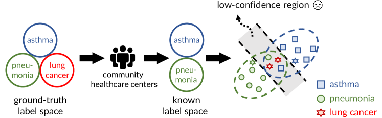
In this paper, we study the task in which there are unknown labels in the training dataset, namely some training instances belonging to a certain class are wrongly perceived as others, and thus appear unknown to the learned model. This is always the case when the label space is misspecified due to the insufficient feature information. Consider the task of medical diagnosis, where we need to train a model for community healthcare centers based on their patient records, to help diagnose the cause of a patient with cough and dyspnea. As shown in Figure 1, there are actually three causes: two common ones (asthma and pneumonia), as well as an unusual one (lung cancer) whose diagnosis crucially relies on the computerized tomography (CT) scan device, yet too expensive to purchase. Thus, the community healthcare centers are not likely to diagnose patients with dyspepsia as cancer, resulting in that the class of “lung cancer” becomes invisible in the collected training dataset, and thus the learned model will be unaware of this unobserved class.

Figure 1: An illustration for the emerging unknown unknowns in the task of medical diagnosis, where the patients with lung cancer are misdiagnosed as asthma or pneumonia due to the lack of CT scan devices, and thus appear as unknown to the learned model.

Similar phenomena occur in many other applications. For instance, the trace of a new-type aircraft was mislabeled as old-type aircrafts until performance of the aircraft detector is found poor (i.e., capability of collected signals is inadequate), and the officer suspects that there are new-type aircrafts unknown previously. When feature information is insufficient, there is a high risk for the learner to misperceive some classes existing in the training data as others, leading to the existence of unknown classes. Especially, unknown classes are sometimes of more interest, like in the above two examples. Therefore, it is crucial for the learned model to discover unknown classes and classify known classes well simultaneously.

However, the conventional supervised learning (SL), where a predictive model is trained on a given labeled dataset and then deployed to classify unseen instances into known labels, crucially relies on a high-quality training dataset. Thus, when the aforementioned unknown unknowns emerged in the training data, SL cannot obtain a satisfied learned model.

2 ExML: A New Learning Framework

The problem we are concerned with is essentially a class of unknown unknowns. In fact, how to deal with unknown unknowns is the fundamental question of the robust artificial intelligence (Dietterich, 2017), and many studies are devoted to addressing various aspects including distribution changes (Pan and Yang, 2010), open category learning (Scheirer et al., 2013), high-confidence false predictions (Attenberg et al., 2015), etc. Different from them, we study a new problem setting ignored previously, that is, the training dataset is badly advised by the incompletely perceived label space due to the insufficient feature information.

The problem turns out to be quite challenging, as feature space and label space are entangled and both of them are unreliable. Notably, it is infeasible to merely pick out instances with low predictive confidence as unknown classes, because we can hardly distinguish two types of low-confidence instances: (i) instances from unknown classes owing to the incomplete label space; (ii) instances from known classes because of insufficient feature information. This characteristic reflects the intrinsic hardness of learning with unknown unknowns due to the feature deficiency, and therefore it is necessary to ask for external feature information.

2.1 Exploratory Machine Learning

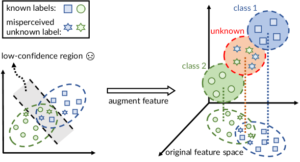
To handle the unknown unknowns caused by the feature deficiency, we resort to the human in the learning loop to actively augment the feature space. The idea is that when a learned model remains performing poorly even fed with many more data, the learner will suspect the existence of unknown classes and subsequently seek several candidate features to augment. Figure 2 shows a straightforward example that the learner receives a dataset and observes there are two classes with poor separability, resulting in a noticeable low-confidence region. After a proper feature augmentation, the learner will then realize that there exists an additional class that is unknown previously due to the insufficient feature information.

Figure 2: An example illustrates that an informative feature can substantially improve the separability of low-confidence samples and make the unknown label distinguishable.

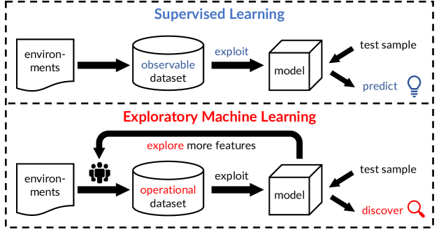
Enlightened by the above example, we introduce a new learning framework called exploratory machine learning (ExML), which explores more feature information to deal with the unknown unknowns caused by feature deficiency. The terminology of exploratory learning is originally raised in the area of education, defined as an approach to teaching and learning that encourages learners to examine and investigate new material with the purpose of discovering relationships between existing background knowledge and unfamiliar content and concepts (Njoo and De Jong, 1993; Spector et al., 2014). In the context of machine learning, our proposed framework encourages learners to examine and investigate the training dataset via exploring new feature information, with the purpose of discovering potentially unknown classes and classifying known classes. Figure 3 compares the proposed ExML to conventional supervised learning (SL). SL views the training dataset as an observable representation of environments and exploits it to train a model to predict the label. By contrast, ExML considers the training dataset is operational, where learners can examine and investigate the dataset by exploring more feature information, and thereby discovers unknown unknowns due to the feature deficiency.

Figure 3: Comparison of two learning frameworks. Supervised learning exploits observable dataset for prediction. Exploratory machine learning explores more features based on operational dataset for both predicting and discovering unknown classes.

We further develop an approach to implement ExML, consisting of three ingredients: rejection model, feature acquisition, and model cascade. The rejection model identifies suspicious instances that potentially belong to unknown classes. Feature acquisition guides which feature should be explored, and then retrains the model on the augmented feature space. Model cascade refines the selection of suspicious instances by cascading rejection models and feature acquisition modules. We present empirical evaluations on synthetic data to illustrate the idea, and provide experimental studies on real datasets to validate the effectiveness of our approach further.

2.2 Problem Formulation

We formalize the problem setting, both training and testing.

Training Dataset. The learner receives a training dataset $\widehat{D}_{tr}=\{(\widehat{\mathbf{x}}_{i},\widehat{\mathbf{y}}_{i})\}_{i=1}^{m}$, where $\widehat{\mathbf{x}}_{i}\in\widehat{\mathcal{X}}\subseteq\mathbb{R}^{d}$ is from the observed feature space, and $\widehat{\mathbf{y}}_{i}\in\widehat{\mathcal{Y}}$ is from the incomplete label space with $N$ known classes. We consider the binary case (i.e., $N=2$) for simplicity. Note that there exist some training samples that are actually from unknown classes yet wrongly labeled as known classes due to the feature deficiency.

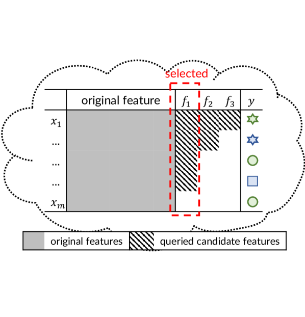
Candidate Features and Cost Budget. Besides the training dataset, the learner can access a set of candidate features $\mathcal{C}=\{c_{1},\ldots,c_{K}\}$, whose values are unknown before acquisition. For the example of medical diagnosis (Figure 1), a feature refers to signals returned from the CT scan devices, only available after patients have taken the examination.

A certain cost will be incurred to acquire any candidate feature for any sample. The learner aims to identify top $k$ informative features from the pool under the given budget $B$. For simplicity, the cost of each acquisition is set as $1$ uniformly and the learner desires to find the best feature, i.e., $k=1$.

Testing Stage. Suppose the learner identifies the best feature as $c_{i}$, she will then augment the testing sample with this feature. Thus, the sample is finally in the augmented feature space $\mathcal{X}_{i}=(\widehat{\mathcal{X}}\cup\mathcal{X}^{i})\subseteq\mathbb{R}^{d+1}$, where $\mathcal{X}^{i}$ is the feature space of $c_{i}$. The learned model requires to predict the label of the augmented testing sample, either classified to one of known classes or discovered as the unknown classes (abbrev. uc).

3 A Practical Approach

Due to the feature deficiency, the learner might be even unaware of the existence of unknown classes based on the observed training data. To address the difficulties, our intuition is that learner will suspect the existence of unknown classes when the learned model performs badly. Therefore, we assume that instances with high predictive confidence are safe, i.e., they will be correctly predicted as one of known classes.

We justify the necessity of the assumption. Actually, there are some previous works studying the problem of high-confidence false predictions (Attenberg et al., 2015; Lakkaraju et al., 2017), under the condition that the feature information is sufficient and learner can query an oracle for ground-truth labels. However, when features are insufficient as in our scenario, the problem would not be tractable unless there is an oracle able to provide exact labels based on the insufficient feature representation, which turns out to be a rather strong assumption that does not hold in reality generally.

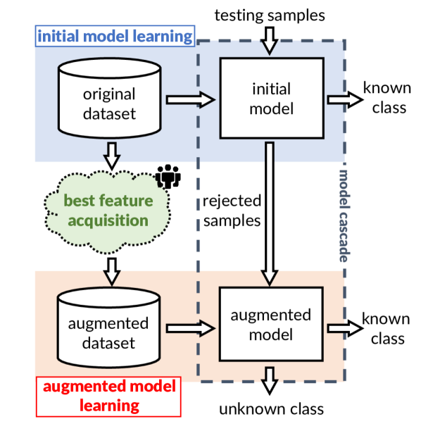
Thereby, following the methodology of ExML (examining the training dataset via exploring new feature information), we design a novel approach, which consists of three components: rejection model, feature acquisition, and model cascade. Figure 4 illustrates main procedures, and we will describe details of each component subsequently.

3.1 Rejection Model

As shown in Figure 4(a), at the beginning, the learner requires to train an initial model on the original dataset, with capability of identifying low-confidence instances as suspicious. We realize this goal by the learning with rejection technique (Cortes et al., 2016a), where the learned model will abstain from predicting instances whose maximum conditional probability is lower than a given threshold $1-\theta$, where $0<\theta<0.5$.

Specifically, we learn a function pair $f=(h,g)$, where $h:\widehat{\mathcal{X}}\mapsto\mathbb{R}$ is the predictive function for known classes and $g:\widehat{\mathcal{X}}\mapsto\mathbb{R}$ is the gate function to reject the unknown class. We predict the sample $\widehat{\mathbf{x}}$ to unknown class if $g(\widehat{\mathbf{x}})<0$, and otherwise to the class of $\mathtt{sign}(h(\widehat{\mathbf{x}}))$. The pair $f=(h,g)$ can be learned by the expected risk minimization,

$$\min_{f}\ \mathbb{E}_{(\widehat{\mathbf{x}},\widehat{y})\sim\widehat{\mathcal{D}}}[\ell_{0/1}(f,\widehat{\mathbf{x}},\widehat{\mathbf{y}};\theta)],$$ (1)

where $\ell_{0/1}(f,\widehat{\mathbf{x}},\widehat{\mathbf{y}};\theta)=\mathds{1}_{\widehat{y}\cdot h(\widehat{\mathbf{x}})<0}\cdot\mathds{1}_{g(\widehat{\mathbf{x}})>0}+\theta\cdot\mathds{1}_{g(\widehat{\mathbf{x}})\leq 0}$ is the 0-1 loss of the rejection model $f$ parameterized by the threshold $\theta$ and $\widehat{\mathcal{D}}$ is the data distribution over $\widehat{\mathcal{X}}\times\widehat{\mathcal{Y}}$.

(a) overall procedure

(b) best feature acquisition

Figure 4: Left figure shows the overall procedure of ExML, which begins with an initial model (blue part), followed by exploring the best candidate feature (green part). Afterwards, a model is retrained based on the augmented dataset, and finally cascaded with the initial model to discover the unknown class (red part). Right figure describes the procedure of best feature acquisition.

Due to the non-convexity arising from the indicator function, the calibrated surrogate loss function $\ell_{surr}(f,\widehat{\mathbf{x}},\widehat{y};\theta)$ is introduced by Cortes et al. (2016a) and defined as

$$\ell_{surr}(f,\widehat{\mathbf{x}},\widehat{y};\theta)=\max\left\{1+\frac{1}{2}\big{(}g(\widehat{\mathbf{x}})-\widehat{y}\cdot h(\widehat{\mathbf{x}})\big{)},\theta\Big{(}1-\frac{g(\widehat{\mathbf{x}})}{1-2\theta}\Big{)},0\right\}$$

to approximate the original $\ell_{0/1}$ loss. Hence, we turn to the empirical risk minimization (ERM) over the surrogate loss,

$$\min_{f\in\mathbb{H}\times\mathbb{H}}~{}~{}\frac{1}{m}\sum_{i=1}^{m}\ell_{surr}(f,\widehat{\mathbf{x}}_{i},\widehat{y}_{i};\theta)+C_{h}\|h\|^{2}_{\mathbb{H}}+C_{g}\|g\|^{2}_{\mathbb{H}},$$ (2)

where $C_{h}$ and $C_{g}$ are regularization parameters, and $\mathbb{H}$ is the reproducing kernel Hilbert space (RKHS) induced by a kernel function $K:\widehat{\mathcal{X}}\times\widehat{\mathcal{X}}\mapsto\mathbb{R}$. According to the representer theorem (Schölkopf and Smola, 2002), the optimal solution of (2) is in the form of $h(\widehat{\mathbf{x}})=\sum_{i=1}^{m}u_{i}K(\widehat{\mathbf{x}},\widehat{\mathbf{x}}_{i})$ and $g(\widehat{\mathbf{x}})=\sum_{i=1}^{m}w_{i}K(\widehat{\mathbf{x}},\widehat{\mathbf{x}}_{i})$, where $u_{i}$ and $w_{i}$ are coefficients to learn. Thus, (2) can be converted into a quadratic programming problem and solved efficiently. Readers can refer to the the seminal work of Cortes et al. (2016a) for more details.

3.2 Feature Acquisition

If the initial model is unqualified (for instance, it rejects too many samples for achieving desired accuracy), learner will suspect the existence of unknown classes and explore new features to augment. In our setting, learner requires to select the best feature from $K$ candidates and retrain a model based on the augmented data, as demonstrated in Figure 4(b). Consequently, the central questions are in the following two aspects:

• how to measure the quality of candidate features?

• how to allocate the budget to identify the best feature and then use the augmented data to retrain the model?

Feature quality measure. Denote by $\mathcal{D}_{i}$ the data distribution over $\mathcal{X}_{i}\times\widehat{\mathcal{Y}}$, where $\mathcal{X}_{i}$ is the augmented feature space of the $i$-th candidate feature, $i\in[K]$. The crucial idea is to use the Bayes risk of rejection model on $\mathcal{D}_{i}$ as the measure

$$R_{i}^{*}=R_{i}(f^{*}_{i})=\min_{f}\ \mathbb{E}_{(\mathbf{x},\widehat{\mathbf{y}})\sim\mathcal{D}_{i}}\big{[}\ell_{0/1}(f,\mathbf{x},\widehat{\mathbf{y}};\theta)\big{]},$$ (3)

where $R_{i}(f)$ is the expected $0/1$ risk of function $f$ over $\mathcal{D}_{i}$, and $f^{*}_{i}$ minimizes $R_{i}(f)$ over all measurable functions. The better the feature is, the lower the Bayes risk should be.

The Bayes risk essentially reflects the minimal error of any rejection model can attain on given features, whose value should be smaller if the feature is more informative.

Due to the inaccessibility of the underlying distribution $\mathcal{D}_{i}$, we approximate the Bayes risk by its empirical version over the augmented data $D_{i}=\{(\mathbf{x}_{j},\widehat{\mathbf{y}}_{j})\}_{j=1}^{n_{i}}\overset{n_{i}}{\sim}\mathcal{D}_{i}$, defined as

$$\widehat{R}_{D_{i}}=\widehat{R}_{i}(\widehat{f}_{i})=\sum_{j=1}^{n_{i}}\ell_{0/1}(\widehat{f}_{i},\mathbf{x}_{j},\widehat{y}_{j};\theta),$$ (4)

where $\mathbf{x}_{j}\in\mathcal{X}_{i},\widehat{\mathbf{y}}_{j}\in\widehat{\mathcal{Y}}$, and $\widehat{f}_{i}$ is the rejection model learned by ERM over the surrogate loss (2) on augmented dataset $D_{i}$.

Based on the feature quality measure (3) and its empirical version (4), we now introduce the budget allocation strategy to identify the best candidate feature.

Budget allocation strategy. Without loss of generality, suppose all the candidate features are sorted according to their quality, namely $R_{1}^{*}\leq\cdots\leq R_{K}^{*}$. Our goal is to identify the best feature within the limited budget, and meanwhile the model retrained on augmented data should have good generalization ability.

To this end, we propose the uniform allocation strategy as follows, under the guidance of the proposed criterion (3).

Uniform Allocation For each candidate feature $c_{i}$, $i\in[K]$, learner allocates $\lfloor B/K\rfloor$ budget and obtains an augmented dataset $D_{i}$. We can thus compute the empirical feature measure by (4), and select the feature with the smallest risk.

The above strategy is simple yet effective. Actually, the approach can identify the best feature with high probability, as will be rigorously demonstrated in Theorem 4.

Median Elimination Besides, we propose another variant inspired by the bandit theory (Lattimore and Szepesvári, 2019) to further improve the budget allocation efficiency. Specifically, we adopt the technique of median elimination (Even-Dar et al., 2006), which removes half of poor candidate features after every iteration and thus avoids allocating too many budgets on poor features. Concretely, we maintain an active candidate feature pool initialized as $\mathcal{C}$ at the beginning and proceed to eliminate half of it for $T=\lceil\log_{2}K\rceil$ episodes. In each episode, $\lfloor B/T\rfloor$ budget is allocated uniformly for all active candidate features, and the augmented datasets $D_{i}$ are updated to accommodate the selected instances. By calculating the empirical feature measure on the augmented dataset, the poor half of the active candidates can be eliminated. The whole algorithm is summarized in Algorithm 1. As shown in Figure 4(b), since poor features are eliminated earlier, the budget left for the selected feature is improved from $\lfloor B/K\rfloor$ to $\lfloor B/\log K\rfloor$ in this way, which ensures better generalization ability of the learned model. Meanwhile, as shown in the bandits literature (Even-Dar et al., 2006), median elimination can also explore the best candidate feature more efficiently than uniform allocation. We currently focus on identifying the best feature, and our framework can be further extended to the scenario of identifying top $k$ features ($k>1$) by introducing more sophisticated techniques in the bandit theory (Kalyanakrishnan et al., 2012; Chen et al., 2017).

Algorithm 1 Median Elimination for Feature Acquisition

0:  Feature acquisition budget $B$, original dataset $\widehat{D}_{tr}$, candidate feature pool $\mathcal{C}=\{c_{1},\ldots,c_{K}\}$, threshold $\theta$.

0:  Selected feature $c_{i_{s}}$ and corresponding model $\widehat{f}_{i_{s}}$.

1:  Initialization: dataset $D_{i}=\varnothing$ for each feature $c_{i}\in\mathcal{C}$, the set of active features $\mathcal{C}_{1}=\mathcal{C}$, $T=\lceil\log_{2}K\rceil$.

2:  for $t=1,\dots,T$ do

3:     Randomly select $n_{t}=\left\lfloor B/(T|\mathcal{C}_{t}|)\right\rfloor$ samples from $\widehat{D}_{tr}$ and query their value of active candidate features $c_{i}\in\mathcal{C}_{t}$;

4:     Update $D_{i}$ to accommodate selected samples and train a model $\widehat{f}_{i}$ on $D_{i}$ by ERM (2), for all active candidate feature $c_{i}\in\mathcal{C}_{t}$;

5:     Compute $\widehat{R}_{D_{i}}$ according to (4), for all $c_{i}\in\mathcal{C}_{t}$;

6:     Update $\mathcal{C}_{t+1}$ as half of features in $\mathcal{C}_{t}$ with lower $\widehat{R}_{D_{i}}$;

7:  end for

3.3 Model Cascade

After feature acquisition, learner will retrain a model on augmented data. Considering that the augmented model might not always better than the initial model, particularly when the budget is not enough or candidate features are not quite informative, we propose the model cascade mechanism to cascade the augmented model with the initial one. Concretely, high-confidence predictions are accepted in the initial model, the rest suspicious are passed to the next layer for feature acquisition, those augmented samples with high confidence will be accepted by the augmented model, and the remaining suspicious continue to the next layer for further refinement.

Essentially, our approach can be regarded as a layer-by-layer processing for identifying unknown classes, and the layers can stop until human discovers remaining suspicious are indeed from certain unknown classes. For simplicity, we only implement a two-layer architecture.

4 Theoretical Analysis

This section presents theoretical results. We first investigate the attainable excess risk of supervised learning, supposing that the best feature were known in advance. Then, we provide the result of ExML to demonstrate the effectiveness of our proposed criterion and budget allocation strategies.

For each candidate feature $c_{i}$, we denote the corresponding hypothesis space as $\mathcal{H}_{i},\mathcal{G}_{i}=\{\mathbf{x}\mapsto\langle\mathbf{w},\Phi_{i}(\mathbf{x})\rangle\mid\lVert\mathbf{w}\rVert_{\mathbb{H}_{i}}\leq\Lambda_{i}\}$, where $\Phi_{i}$ and $\mathbb{H}_{i}$ are induced feature mapping and RKHS of kernel $K_{i}$ in the augmented feature space.

Supervised learning with known best feature. Suppose the best feature is known in advance, we can obtain $B$ samples augmented with this particular feature. Let $f_{\text{SL}}$ be the model learned by supervised learning via minimizing (2). From learning theory literatures (Bousquet et al., 2003; Mohri et al., 2018), for any $\delta>0$, with probability at least $1-\delta$, the excess risk is bounded by

$$R_{1}(f_{\text{SL}})-R_{1}^{*}\leq\mathcal{O}\bigg{(}\sqrt{\frac{(\kappa_{1}\Lambda_{1})^{2}}{B}}+\sqrt{\frac{\log(1/\delta)}{2B}}\bigg{)}+R_{ap},$$ (5)

where $R_{ap}=C_{\theta}\left(\inf_{f\in\mathcal{H}_{1}\times\mathcal{G}_{1}}R^{surr}_{1}(f)-\inf_{f}R^{surr}_{1}(f)\right)$ is the approximation error measuring how well hypothesis spaces $\mathcal{H}_{1}$, $\mathcal{G}_{1}$ approach the target, in terms of the expected surrogate risk $R_{1}^{surr}(f)=\mathbb{E}_{(\mathbf{x},\widehat{\mathbf{y}})\sim\mathcal{D}_{1}}[\ell_{surr}(f,\mathbf{x},\widehat{\mathbf{y}};\theta)]$. The constant factor is $C_{\theta}=1/((1-\theta)\cdot(1-2\theta))$.

Thus, when the best feature is known in advance and given the budget $B$, excess risk of supervised learning converges to the inevitable approximate error in the rate of $\mathcal{O}(1/\sqrt{B})$.

Exploratory learning with unknown best feature. In reality, the best feature is unfortunately unknown ahead of time and $K$ candidate features are available. We show that by means of ExML, the excess risk also converges, in the rate of $\mathcal{O}(\sqrt{K/B})$, yet without requiring to know the best feature. Let $c_{i_{s}}$ be the identified feature and $\widehat{f}_{i_{s}}$ be the augmented model returned by ExML with uniform allocation on kernel based hypotheses. Then, with probability at least $1-\delta$, we have

$$R_{i_{s}}(\widehat{f}_{i_{s}})-R_{1}^{*}\leq C_{\theta}^{\prime}\cdot\sqrt{\frac{(\kappa\Lambda)^{2}}{\lfloor B/K\rfloor}}+2(1+C_{\theta}B)\sqrt{\frac{\log(6/\delta)}{2\lfloor B/K\rfloor}}+R_{ap},$$ (6)

where $\Lambda=\sup_{i\in[K]}\Lambda_{i}$ and $\kappa=\sup_{i\in[K]}\sup_{\mathbf{x}\in\mathcal{X}_{i}}K_{i}(\mathbf{x},\mathbf{x})$. The constant $C_{\theta}^{\prime}=4+2\theta+\frac{4}{(1-2\theta)^{2}}$ and $B=1+\max\big{\{}1,\frac{\theta}{1-2\theta}\big{\}}\cdot\kappa\Lambda$.

Compared with excess risk bounds of (5) and (6), we can observe that ExML exhibits a similar convergence rate of SL with known best feature, yet without requiring to know the best feature. An extra $\sqrt{K}$ times factor is paid for best feature identification. We note that under certain mild technical assumptions, the dependence can be further improved to $\sqrt{\log K}$ by median elimination (Even-Dar et al., 2006), as poor candidate features are removed in earlier episodes.

Proof of Theorem 4.

The excess risk of the learned model $\widehat{f}_{i_{s}}$ can be decomposed into three parts,

$$\begin{split}R_{i_{s}}(\widehat{f}_{i_{s}})-R_{1}^{*}&=\underbrace{R_{i_{s}}(\widehat{f}_{i_{s}})-\widehat{R}_{i_{s}}(\widehat{f}_{i_{s}})}_{\mathtt{term~{}(a)}}+\underbrace{\widehat{R}_{i_{s}}(\widehat{f}_{i_{s}})-\widehat{R}_{1}(\widehat{f}_{1})}_{\mathtt{term~{}(b)}}+\underbrace{\widehat{R}_{1}(\widehat{f}_{1})-R_{1}^{*}}_{\mathtt{term~{}(c)}},\end{split}$$

where $\mathtt{term~{}(a)}$ is the generalization error of the learned model $\widehat{f}_{i_{s}}$ and $\mathtt{term~{}(b)}$ is the difference between empirical criterion of the selected feature and that of the best feature, where $\widehat{f}_{1}$ refers to the model trained on the best feature with a $\lfloor B/K\rfloor$ budget. Besides, $\mathtt{term~{}(c)}$ captures the excess risk of $\widehat{f}_{1}$ relative to the Bayes risk. Notice that $\mathtt{term~{}(b)}<0$ since the empirical criterion of the selected feature is the lowest among all candidates. Thus, to prove the theorem, it is sufficient to bound $\mathtt{term~{}(a)}$ and $\mathtt{term~{}(c)}$.

We bound $\mathtt{term}~{}(a)$ based on the following lemma on the generalization error of the rejection model, which can be regarded as a two-side counterpart of Theorem 1 of Cortes et al. (2016a). Let $\mathcal{H}$ and $\mathcal{G}$ be the kernel-based hypotheses $\mathcal{H},\ \mathcal{G}=\{\mathbf{x}\mapsto\langle\mathbf{w},\Phi(\mathbf{x})\rangle|\|\mathbf{w}\|_{\mathbb{H}}\leq\Lambda\}$. Then for any $\delta>0$, with probability of $1-\delta$ over the draw of a sample $D$ of size $n$ from $\mathcal{D}$, the following holds for all $f\in\mathcal{H}\times\mathcal{G}$:

$$|R(f)-\widehat{R}(f)|\leq(2+\theta)\sqrt{\frac{(\kappa\Lambda)^{2}}{n}}+\sqrt{\frac{\log(2/\delta)}{2n}},$$ (7)

where $\kappa^{2}=\sup_{\mathbf{x}\in\mathcal{X}}K(\mathbf{x},\mathbf{x})$ and $K:\mathcal{X}\times\mathcal{X}\mapsto\mathbb{R}$ is the kernel function associated with $\mathbb{H}$. Therefore, the generalization error of the $\widehat{f}_{i_{s}}$ can be directly bounded by,

$$\mathtt{term~{}(a)}\leq(2+\theta)\sqrt{\frac{(\kappa_{s}\Lambda_{s})^{2}}{\lfloor B/K\rfloor}}+\sqrt{\frac{\log(2/\delta^{\prime})}{2\lfloor B/K\rfloor}},$$ (8)

with probability at least $1-\delta^{\prime}$.

Then we process to analyze the excess risk of $\widehat{f}_{1}$ trained on the best feature with surrogate loss $\ell_{surr}$, where $\mathtt{term~{}(c)}$ can be decomposed into two parts as

$$\mathtt{term~{}(c)}=\widehat{R}_{1}(\widehat{f}_{1})-R_{1}^{*}=\underbrace{\widehat{R}_{1}(\widehat{f}_{1})-R_{1}(\widehat{f}_{1})}_{\mathtt{term~{}(c\text{-}1)}}+\underbrace{R_{1}(\widehat{f}_{1})-R_{1}^{*}}_{\mathtt{term~{}(c\text{-}2)}}.$$

Based on Lemma 4, $\mathtt{term~{}(c\text{-}1)}$ is bounded by,

$$\begin{split}\mathtt{term~{}(c\text{-}1)}\leq(2+\theta)\sqrt{\frac{(\kappa_{1}\Lambda_{1})^{2}}{\lfloor B/K\rfloor}}+\sqrt{\frac{\log(2/\delta^{\prime})}{2\lfloor B/K\rfloor}},\end{split}$$ (9)

with probability at least $1-\delta^{\prime}$.

Before presenting the analysis on $\mathtt{term~{}(c\text{-}2)}$, we introduce the results on consistency and the generalization error of the surrogate loss function. First, we show that the excess risk with respect to 0/1 loss for any function $f$ is bound by the excess risk with respect to the surrogate loss $\ell_{surr}$.

[Theorem 3 of Cortes et al. (2016a)] Let $R^{surr}(f)=\mathbb{E}_{(\mathbf{x},y)\sim\mathcal{D}}[\ell_{surr}(f,\mathbf{x},y;\theta)]$ denote the expected risk in terms of the surrogate loss of a pair $f=(h,g)$. Then, the excess error of $f$ is upper bounded by its surrogate excess error as follows,

$$R(f)-R^{*}\leq C_{\theta}\left(R^{surr}(f)-\inf_{f}R^{surr}(f)\right),$$

where $C_{\theta}=\frac{1}{(1-\theta)(1-2\theta)}$ and $R^{*}=\inf_{f}R(f)$.

Besides, the generalization error of the surrogate loss is as follows, Let $\mathcal{H}$ and $\mathcal{G}$ be the kernel-based hypotheses, defined as $\mathcal{H},\ \mathcal{G}=\{\mathbf{x}\mapsto\langle\mathbf{w},\Phi(\mathbf{x})\rangle|\|\mathbf{w}\|_{\mathbb{H}}\leq\Lambda\}$. Then for any $\delta>0$, with probability of $1-\delta$ over the draw of a sample $D$ of size $n$ from $\mathcal{D}$, the following holds for all $f\in\mathcal{H}\times\mathcal{G}$:

$$|R^{surr}(f)-\widehat{R}^{surr}(f)|\leq\frac{2-2\theta}{1-2\theta}\sqrt{\frac{(\kappa\Lambda)^{2}}{n}}+B\sqrt{\frac{\log(2/\delta)}{2n}},$$ (10)

where $\kappa^{2}=\sup_{\mathbf{x}\in\mathcal{X}}K(\mathbf{x},\mathbf{x})$ and $K:\mathcal{X}\times\mathcal{X}\mapsto\mathbb{R}$ is the kernel function associated with $\mathbb{H}$. $B=\sup_{f\in\mathcal{H}\times\mathcal{G}}\sup_{(\mathbf{x},y)\in\mathcal{X}\times\mathcal{Y}}\ell_{surr}(f,\mathbf{x},y;\theta)\leq 1+\max\left\{1,\frac{\theta}{1-2\theta}\right\}\cdot\kappa\Lambda$. Lemma 4 can be obtained by the standard analysis of generalization error based on the Rademacher complexity (Mohri et al., 2018).

Based on the consistency of the surrogate loss function shown in Lemma 4, we have

$$\begin{split}{}&\mathtt{term~{}(c\text{-}2)}\\ \leq{}&C_{\theta}\big{(}R_{1}^{surr}(\widehat{f}_{1})-\inf\nolimits_{f}R_{1}^{surr}(f)\big{)}\\ ={}&C_{\theta}\left(R_{1}^{surr}(\widehat{f}_{1})-\inf_{f\in\mathcal{H}_{1}\times\mathcal{G}_{1}}R_{1}^{surr}(f)+\inf_{f\in\mathcal{H}_{1}\times\mathcal{G}_{1}}R_{1}^{surr}(f)-\inf_{f}R_{1}^{surr}(f)\right)\\ ={}&C_{\theta}\left(R_{1}^{surr}(\widehat{f}_{1})-\inf_{f\in\mathcal{H}_{1}\times\mathcal{G}_{1}}R_{1}^{surr}(f)\right)+R_{ap}.\end{split}$$ (11)

Denote $f_{1}^{*}=\inf_{f\in\mathcal{H}_{1}\times\mathcal{G}_{1}}R_{1}^{surr}(f)$, the first term of (12) can be further bounded by the generalization error bound of the the surrogate loss function and the optimality of $\widehat{f}_{1}$ for the ERM problem (2) in hypotheses $\mathcal{H}_{1}\times\mathcal{G}_{1}$ as,

$$R_{1}^{surr}(\widehat{f}_{1})-R_{1}^{surr}(f_{1}^{*})$$

$$={} R_{1}^{surr}(\widehat{f}_{1})-\widehat{R}_{1}^{surr}(\widehat{f}_{1})+\widehat{R}_{1}^{surr}(\widehat{f}_{1})-R_{1}^{surr}(f_{1}^{*})$$

$$\leq{} R_{1}^{surr}(\widehat{f}_{1})-\widehat{R}_{1}^{surr}(\widehat{f}_{1})+\widehat{R}_{1}^{surr}(f_{1}^{*})-R_{1}^{surr}(f_{1}^{*})$$

$$\leq{} 2\sup_{f\in\mathcal{H}_{1}\times\mathcal{G}_{1}}|R_{1}^{surr}(f)-\widehat{R}_{1}^{surr}(f)|$$

$$\leq{} \frac{4-4\theta}{1-2\theta}\sqrt{\frac{(\kappa_{1}\Lambda_{1})^{2}}{\lfloor B/K\rfloor}}+2B\sqrt{\frac{\log(2/\delta^{\prime})}{2\lfloor B/K\rfloor}}.$$

Thus, the following inequality

$$\begin{split}{}&\mathtt{term~{}(c\text{-}2)}\leq C_{\theta}\left(\frac{4-4\theta}{1-2\theta}\sqrt{\frac{(\kappa_{1}\Lambda_{1})^{2}}{\lfloor B/K\rfloor}}+2B\sqrt{\frac{\log(2/\delta^{\prime})}{2\lfloor B/K\rfloor}}\right)+R_{ap}\end{split}$$ (12)

satisfies with probability at least $1-\delta^{\prime}$.

Taking $\kappa=\sup_{i\in[K]}\kappa_{i}$, $\Lambda=\sup_{i\in[K]}\Lambda_{i}$ and $\delta^{\prime}=\delta/3$, we complete the proof by combining (8), (9), and (12), obtaining that

$$\begin{split}{}&R_{i_{s}}(\widehat{h}_{i_{s}},\widehat{g}_{i_{s}})-R_{1}^{*}\\ \leq{}&(4+2\theta)\sqrt{\frac{(\kappa\Lambda)^{2}}{\lfloor B/K\rfloor}}+2\sqrt{\frac{\log(6/\delta)}{2\lfloor B/K\rfloor}}+C_{\theta}\left(\frac{4-4\theta}{1-2\theta}\sqrt{\frac{(\kappa\Lambda)^{2}}{\lfloor B/K\rfloor}}+2B\sqrt{\frac{\log(6/\delta)}{2\lfloor B/K\rfloor}}\right)+R_{ap}\\ ={}&\bigg{(}4+2\theta+\frac{4}{(1-2\theta)^{2}}\bigg{)}\sqrt{\frac{(\kappa\Lambda)^{2}}{\lfloor B/K\rfloor}}+2(1+C_{\theta}B)\sqrt{\frac{\log(6/\delta)}{2\lfloor B/K\rfloor}}+R_{ap}\end{split}$$

holds with probability at least $1-\delta$. ∎

5 Related Work

In this section, we discuss some related topics.

Open Category Learning is also named as learning with new classes, which focuses on handling unknown classes appearing only in the testing phase (Scheirer et al., 2013, 2014; Da et al., 2014; Mendes-Junior et al., 2017; Liu et al., 2018; Zhang et al., 2019). Although these studies also care about the unknown classes detection, they differ from us significantly and thus cannot apply to our situation: first, they do not consider the feature deficiency; second, there exist unknown classes in training data in our setting, while theirs only appear in the testing.

High-Confidence False Predictions appear due to model’s unawareness of such kind of mistake (Attenberg et al., 2015; Lakkaraju et al., 2017; Bansal and Weld, 2018). To handle such unknown unknowns, existing studies typically ask for external human expert to help identifying high-confidence false predictions and then retrain the model with the guidance. Although these works also consider unknown unknowns and resort to external human knowledge, their setting and methodology differ from ours: our unknown unknowns are caused due to the feature deficiency, so the learner requires to augment features rather than querying the labels.

Active Learning aims to achieve greater accuracy with fewer labels by asking queries of unlabeled data to be labeled by the human expert (Settles, 2012). Besides, there are some works querying features (Melville et al., 2005; Dhurandhar and Sankaranarayanan, 2015; Huang et al., 2018), which tries to improve learning with missing features via as fewer as possible queries of entry values (feature of an instance). Unlike their setting, we augment new features to help the identification of the unknown classes rather than querying missing values of the given feature to improve the performance of known classes classification.

Learning with Rejection gives the classifier an option to reject an instance instead of providing a low-confidence prediction (Chow, 1970). Plenty of works are proposed to design effective algorithms (Yuan and Wegkamp, 2010; Cortes et al., 2016b; Wang and Qiao, 2018; Shim et al., 2018) and establish theoretical foundations (Herbei and Wegkamp, 2006; Bartlett and Wegkamp, 2008; Cortes et al., 2016a; Bousquet and Zhivotovskiy, 2019). As aforementioned, methods of rejection cannot be directly applied in exploratory machine learning since it will result in inaccurate rejections of instances from known classes, and meanwhile, it cannot exploit new features.

6 Experiments

We conduct experiments on both synthetic and real datasets to evaluate exploratory learning in the following aspects:

• advantage of exploratory learning over conventional supervised learning in handling unknown unknowns;

• effectiveness of the proposed ExML approach, and the usefulness of feature acquisition and model cascade.

We choose kernel support vector machine as the base model with Gaussian kernel $K(\mathbf{x}_{i},\mathbf{x}_{j})=\exp(-\|\mathbf{x}_{i}-\mathbf{x}_{j}\|^{2}_{2}/\gamma)$, and the bandwidth $\gamma$ is set as $\gamma=\mbox{median}_{\mathbf{x}_{i},\mathbf{x}_{j}\in D}(\|\mathbf{x}_{i}-\mathbf{x}_{j}\|_{2}^{2})$. Besides, parameters $C_{h}$, $C_{g}$ are set as $1$. We select the best rejection threshold $\theta$ of augmented model from the pool $[0.1,0.2,0.3,0.4]$ for each algorithm, and the rejection threshold of the initial model is selected by cross validation to ensure 95% accuracy on high-confidence predictions. The feature acquisition budget is set as $B=b\cdot mK$, where $m$ is number of training samples, $K$ is number of candidate features, $b\in[0,1]$ is the budget ratio.

6.1 Synthetic Data for Illustration

We first illustrate the advantage of exploratory machine learning by comparing ExML with SL on the synthetic data.

(a) ground-truth

(b) training data

(c) candidates

Figure 5: Visualization of synthetic data: (a) shows the ground-truth distribution; (b) presents training data (only first two dims are observable); (c) plots $t$-sne of candidate features with various qualities (the larger the angle is, the better the feature is).

(a) SL

(b) ExML

(c) allocation

Figure 6: (a), (b) show performance comparison of SL and ExML; (c) reports budget allocation of ExML with median elimination.

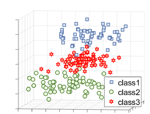
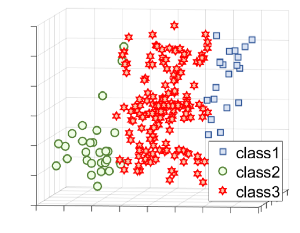
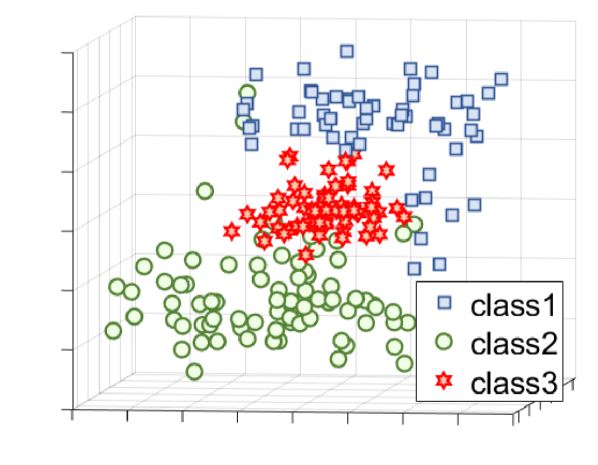
Setting. Following the illustrative example in Figure 1, we generate data with $3$-dim feature and $3$ classes, each class has $100$ samples. Figure 5(a) presents the ground-truth distribution. In detail, instances from each class are generated from a 3-dim Gaussian distributions. The means and variances are $[-a,0,-z]$ and $\sigma\cdot\mathbf{I}_{3\times 3}$ for class 1, $[a,0,z]$ and $\sigma\cdot\mathbf{I}_{3\times 3}$ for class 2 as well as $[0,0,0]$ and $\sigma/2\cdot\mathbf{I}_{3\times 3}$ for class 3, where $\mathbf{I}_{3\times 3}$ is a $3\times 3$ identity matrix. We fix $\sigma=3a$ and set $z=5a$.

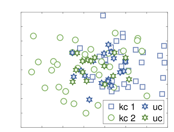
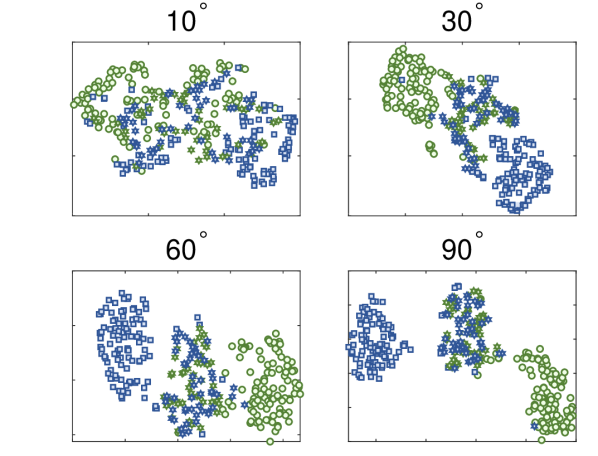
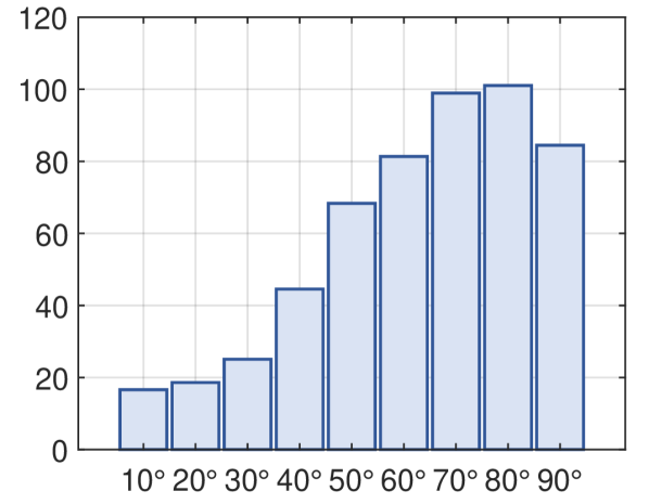
However, as shown in Figures 5(b), the third-dim feature is unobservable in training data, resulting in an unknown class (uc) located in the intersection area of known classes (kc1 and kc2). Samples from uc are mislabeled as kc1 or kc2 randomly. Besides, to generate candidate features in various qualities, we project the third-dim feature to different located in the XZ-plane with angles to horizon varies from $10^{\circ}$ to $90^{\circ}$, the larger the better. We plot four of them in Figure 5(c) via $t$-sne. The budget ratio is set as $b=20\%$.

Results. We first conduct SL to train a rejection model based on the $2$-dim training data, and then perform ExML to actively augment the feature within the budget to discover unknown unknowns. Figures 6(a) and 6(b) plot the results, demonstrating a substantial advantage of ExML over SL in identifying unknown class and predicting known classes.

Furthermore, Figure 6(c) reports the budget allocation of each candidate feature over $50$ times repetition. We can see that the allocation evidently concentrates to the more informative features (with larger angles), validating that the effectiveness of the strategy for best feature identification.

6.2 Benchmark Data for Evaluation

We further evaluate on a UCI dataset Mfeat (van Breukelen et al., 1998), which is a multi-view dataset containing 2000 instances for 10 handwritten number uniformly. Six views of features are extracted by various method for representing the raw data and are of different qualities. We list the detailed description for these features in Table 1 and sort them in the descending order of their own qualities: Fac $>$ Pix $>$ Kar $>$ Zer $>$ Fou $>$ Mor.

Table 1: Evaluation on Mefeat dataset. Features are sorted in descending feature quality. Bold font indicates algorithms significantly outperforms than others (paired $t$-test at 95% significance level).

Feature	Description	Budget	SL	ExML${}_{\text{aug}}^{\text{ME}}$	ExML${}_{\text{csd}}^{\text{UA}}$	ExML	Recall
Fac	Profile correlations	10%	93.39 $\pm$ 1.66	71.80 $\pm$ 9.55	92.39 $\pm$ 2.79	92.40 $\pm$ 2.78	48%
		20%	93.39 $\pm$ 1.66	82.26 $\pm$ 7.52	91.95 $\pm$ 3.32	92.00 $\pm$ 3.27	46%
		30%	93.39 $\pm$ 1.66	89.29 $\pm$ 4.72	92.20 $\pm$ 3.33	92.50 $\pm$ 2.86	44%
Pix	Pixel averages in 2 $\times$ 3 windows	10%	92.19 $\pm$ 2.47	70.53 $\pm$ 8.27	90.54 $\pm$ 6.27	90.55 $\pm$ 6.31	58%
		20%	92.19 $\pm$ 2.47	81.70 $\pm$ 7.16	90.84 $\pm$ 6.17	90.87 $\pm$ 6.09	54%
		30%	92.19 $\pm$ 2.47	88.67 $\pm$ 4.14	90.45 $\pm$ 5.74	91.82 $\pm$ 4.26	68%
Kar	Karhunen-Love coefficients	10%	86.87 $\pm$ 3.43	70.25 $\pm$ 10.2	85.55 $\pm$ 4.94	85.90 $\pm$ 4.85	56%
		20%	86.87 $\pm$ 3.43	81.46 $\pm$ 6.88	85.21 $\pm$ 5.46	86.49 $\pm$ 4.81	54%
		30%	86.87 $\pm$ 3.43	86.01 $\pm$ 5.41	86.52 $\pm$ 4.71	88.18 $\pm$ 3.57	56%
Zer	Zernike moments	10%	73.82 $\pm$ 8.82	69.61 $\pm$ 10.7	72.96 $\pm$ 10.4	76.17 $\pm$ 8.52	82%
		20%	73.82 $\pm$ 8.82	80.86 $\pm$ 8.02	77.31 $\pm$ 7.89	81.72 $\pm$ 7.33	82%
		30%	73.82 $\pm$ 8.82	86.07 $\pm$ 5.51	81.11 $\pm$ 6.79	86.33 $\pm$ 5.04	86%
Fou	Fourier coefficients	10%	68.73 $\pm$ 9.07	69.42 $\pm$ 9.68	68.88 $\pm$ 11.8	75.92 $\pm$ 8.81	82%
		20%	68.73 $\pm$ 9.07	82.11 $\pm$ 6.48	77.93 $\pm$ 8.27	85.03 $\pm$ 4.39	88%
		30%	68.73 $\pm$ 9.07	89.90 $\pm$ 3.69	82.45 $\pm$ 5.20	89.35 $\pm$ 3.89	92%
Mor	Morphological features	10%	57.47 $\pm$ 15.3	69.09 $\pm$ 11.3	66.58 $\pm$ 13.5	71.07 $\pm$ 11.1	80%
		20%	57.47 $\pm$ 15.3	79.60 $\pm$ 10.1	73.61 $\pm$ 8.86	79.74 $\pm$ 9.92	84%
		30%	57.47 $\pm$ 15.2	87.44 $\pm$ 7.34	78.31 $\pm$ 9.00	86.98 $\pm$ 7.07	90%

Setting. To understand ExML better, we compare algorithms in various environments, where each one of six views of features is taken as original feature and the rest are prepared as candidate features. We vary the budget ratio from 5% to 30%. Since Mfeat is a multi-class dataset, we randomly sample 5 configurations to convert it into the binary situation, where each known classes and the unknown class contains three original classes. The training dataset contains 600 instances and 1200 instances are used for testing. For each configuration, training instances are randomly sampled 10 times. The results on accuracy are reported over the 50 times repetition.

Contenders and Measure. Apart from the conventional supervised learning (SL), we include two variants of ExML: ExML${}_{\text{csd}}^{\text{UA}}$ and ExML${}_{\text{aug}}^{\text{ME}}$, to examine the usefulness of model cascade, where aug/csd denotes the model trained on augmented feature space with or without cascade structure, and UA/ME refers to the strategy of feature acquisition, uniform allocation or median elimination. Note that our approach ExML is essentially ExML${}_{\text{csd}}^{\text{ME}}$.

Besides, we introduce the recall of best feature identification to measure the effectiveness of the feature acquisition, defined as the rate of the number of cases when the identified feature is among one of its top 2 features to the total number. For each original feature, the top candidate is measured by the attainable accuracy of the augmented model trained on the whole training dataset with this particular feature when $\theta=0.3$.

Results. Table 1 reports mean and standard deviation of the predictive accuracy, and all features are sorted in descending order by their quality. We first compare SL to (variants of) ExML. When the original features are in high quality (Kar, Pix, Fac), SL could achieve favorable performance and there is no need to explore new features. However, in the case where uninformative original features are provided, which is of more interest for ExML, SL degenerates severely and ExML${}_{\text{aug}}^{\text{ME}}$ (the single ExML model without model cascade) achieves better performance even with the limited budget. Besides, from the last column of the table, we can see that informative candidates (top 2) are selected to strengthen the poor original features, which validates the efficacy of the proposed budget allocation strategy.

Since the ExML${}_{\text{aug}}^{\text{ME}}$ is not guaranteed to outperform SL, particularly with the limited budget on poor candidate features, we propose the cascade structure. Actually, ExML approach (aka, ExML${}_{\text{csd}}^{\text{ME}}$) achieves roughly best-of-two-worlds performance, in the sense that it is basically no worse or even better than the best of SL and ExML${}_{\text{aug}}^{\text{ME}}$. It turns out that even ExML${}_{\text{csd}}^{\text{UA}}$ could behave better than ExML${}_{\text{aug}}^{\text{ME}}$ when the candidate features are uninformative. These results validate the effectiveness of the model cascade component.

6.3 Real Data of Activities Recognition

We additionally conduct experiment on the RealDisp dataset of activities recognition task (Baños et al., 2012), where 9 on-body sensors are used to capture various actions of participants. Each sensors is placed on different parts of the body and provides 13-dimensional features including 3-dim from acceleration, 3-dim from gyro, 3-dim from magnetic field orientation and another 4-dim from quaternions. Hence, we have 117 features in total.

Setting. In our experiments, three types of actions (walking, running, and jogging) are included to form the dataset containing 2000 instances, where 30% of them are used for training and 70% for testing. In the training data, one sensor is deployed and the class of jogging is mispercevied as walking or running randomly. The learner would explore the rest eight candidate features to discover the unknown unknowns. Thus, there are 9 partitions, and each is repeated for 10 times by sampling the training instances randomly.

6cm

Figure 7: Performance comparisons of all the contenders.

6cm

Figure 8: Illustration of budget allocation with median elimination.

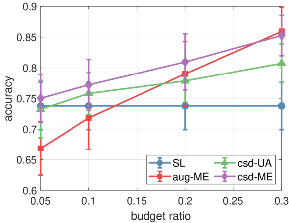
Results. Figure 8 shows the mean and std of accuracy, our approach ExML (aka, ExML${}_{\text{csd}}^{\text{ME}}$) outperforms others, validating the efficacy of our proposal.

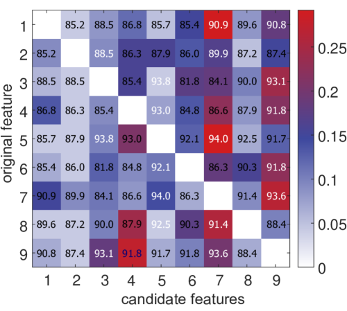
In addition, Figure 8 illustrates the budget allocation when the budget ratio $b=30\%$. The $i$-th row denotes the scenario when the $i$-th sensor is the original feature, and patches with colors indicate the fraction of budget allocated to each candidate feature. The number above a patch means the attainable accuracy of the model trained on the whole training dataset with the particular feature. We highlight the top two candidate features of each row in white, and use blue color to indicate selected feature is not in top two. The results show that ExML with median elimination can select the top two informative features to augment for all the original sensor. The only exception is the 9-th sensor, but quality of the selected feature (91.8$\%$) does not deviate too much from the best one (93.6$\%$). These results reflect the effectiveness of our feature acquisition strategy.

7 Conclusion

This paper studies the task of learning with unknown unknowns, where there exist some instances in training datasets belonging to a certain unknown class but are wrongly perceived as known classes, due to the insufficient feature information. To address this issue, we propose the exploratory machine learning (ExML) to encourage the learner to examine and investigate the training dataset by exploring more features to discover potentially unknown classes. Following this idea, we design an approach consisting of three procedures: rejection model, feature acquisition, and model cascade. By leveraging techniques from bandit theory, we prove the rationale and efficacy of the feature acquisition procedure. Experiments validate the effectiveness of our approach.

There remain many directions worthy exploring for the exploratory machine learning. The first is to further refine the description of human ability in the learning loop. We currently focus on the low-confidence unknown unknowns by requesting humans provide candidate features, and it is interesting to further investigate the high-confidence unknown unknowns by means of asking humans for more information. The second is to consider a personalized cost for each candidate feature, since we usually need to pay a higher price to obtain more informative features in real-world applications. The learner should balance trade-off between accuracy and cost budget. In addition, as mentioned earlier, we will consider the top $k$ feature acquisition if the learner can afford more devices in the testing time, where feature correlations should be taken in account.

References

- Attenberg et al. [2015] J. Attenberg, P. Ipeirotis, and F. Provost. Beat the machine: Challenging humans to find a predictive model’s unknown unknowns. ACM Journal of Data and Information Quality, pages 1–17, 2015.
- Baños et al. [2012] O. Baños, M. Damas, H. Pomares, I. Rojas, M. A. Tóth, and O. Amft. A benchmark dataset to evaluate sensor displacement in activity recognition. In Proceedings of 12th ACM Conference on Ubiquitous Computing (Ubicomp), pages 1026–1035, 2012.
- Bansal and Weld [2018] G. Bansal and D. S. Weld. A coverage-based utility model for identifying unknown unknowns. In Proceedings of the 32nd AAAI Conference on Artificial Intelligence (AAAI), pages 1463–1470, 2018.
- Bartlett and Wegkamp [2008] P. L. Bartlett and M. H. Wegkamp. Classification with a reject option using a hinge loss. Journal of Machine Learning Research, pages 1823–1840, 2008.
- Bousquet and Zhivotovskiy [2019] O. Bousquet and N. Zhivotovskiy. Fast classification rates without standard margin assumptions. arXiv preprint, arXiv:1910.12756, 2019.
- Bousquet et al. [2003] O. Bousquet, S. Boucheron, and G. Lugosi. Introduction to statistical learning theory. In Advanced Lectures on Machine Learning (Machine Learning Summer Schools 2003), pages 169–207, 2003.
- Chen et al. [2017] L. Chen, J. Li, and M. Qiao. Nearly instance optimal sample complexity bounds for top-k arm selection. In Proceedings of the 20th International Conference on Artificial Intelligence and Statistics (AISTATS), pages 101–110, 2017.
- Chow [1970] C. K. Chow. On optimum recognition error and reject tradeoff. IEEE Transactions on Information Theory, pages 41–46, 1970.
- Cortes et al. [2016a] C. Cortes, G. DeSalvo, and M. Mohri. Learning with rejection. In Proceedings of International Conference on Algorithmic Learning Theory (ALT), pages 67–82, 2016a.
- Cortes et al. [2016b] C. Cortes, G. DeSalvo, and M. Mohri. Boosting with abstention. In Advances in Neural Information Processing Systems 29 (NIPS), pages 1660–1668, 2016b.
- Da et al. [2014] Q. Da, Y. Yu, and Z.-H. Zhou. Learning with augmented class by exploiting unlabeled data. In Proceedings of the 28th AAAI Conference on Artificial Intelligence (AAAI), pages 1760–1766, 2014.
- Dhurandhar and Sankaranarayanan [2015] A. Dhurandhar and K. Sankaranarayanan. Improving classification performance through selective instance completion. Machine Learning, pages 425–447, 2015.
- Dietterich [2017] T. G. Dietterich. Steps toward robust artificial intelligence. AI Magazine, pages 3–24, 2017.
- Even-Dar et al. [2006] E. Even-Dar, S. Mannor, and Y. Mansour. Action elimination and stopping conditions for the multi-armed bandit and reinforcement learning problems. Journal of Machine Learning Research, 7:1079–1105, 2006.
- Herbei and Wegkamp [2006] R. Herbei and M. H. Wegkamp. Classification with reject option. Canadian Journal of Statistics, pages 709–721, 2006.
- Huang et al. [2018] S. Huang, M. Xu, M. Xie, M. Sugiyama, G. Niu, and S. Chen. Active feature acquisition with supervised matrix completion. In Proceedings of the 24th ACM SIGKDD International Conference on Knowledge Discovery & Data Mining (KDD), pages 1571–1579, 2018.
- Kalyanakrishnan et al. [2012] S. Kalyanakrishnan, A. Tewari, P. Auer, and P. Stone. PAC subset selection in stochastic multi-armed bandits. In Proceedings of the 29th International Conference on Machine Learning (ICML), 2012.
- Lakkaraju et al. [2017] H. Lakkaraju, E. Kamar, R. Caruana, and E. Horvitz. Identifying unknown unknowns in the open world: Representations and policies for guided exploration. In Proceedings of the 31st AAAI Conference on Artificial Intelligence (AAAI), pages 2124–2132, 2017.
- Lattimore and Szepesvári [2019] T. Lattimore and C. Szepesvári. Bandit Algorithms. Cambridge University Press, 2019.
- Liu et al. [2018] S. Liu, R. Garrepalli, T. G. Dietterich, A. Fern, and D. Hendrycks. Open category detection with PAC guarantees. In Proceedings of the 35th International Conference on Machine Learning (ICML), pages 3175–3184, 2018.
- Melville et al. [2005] P. Melville, F. J. Provost, and R. J. Mooney. An expected utility approach to active feature-value acquisition. In Proceedings of the 5th IEEE International Conference on Data Mining (ICDM), pages 745–748, 2005.
- Mendes-Junior et al. [2017] P. R. Mendes-Junior, R. M. de Souza, R. de Oliveira Werneck, B. V. Stein, D. V. Pazinato, W. R. de Almeida, O. A. B. Penatti, R. da Silva Torres, and A. Rocha. Nearest neighbors distance ratio open-set classifier. Machine Learning, pages 359–386, 2017.
- Mohri et al. [2018] M. Mohri, A. Rostamizadeh, and A. Talwalkar. Foundations of Machine Learning. The MIT Press, second edition, 2018.
- Njoo and De Jong [1993] M. Njoo and T. De Jong. Exploratory learning with a computer simulation for control theory: Learning processes and instructional support. Journal of research in science teaching, pages 821–844, 1993.
- Pan and Yang [2010] S. J. Pan and Q. Yang. A survey on transfer learning. IEEE Transactions on Knowledge and Data Engineering, pages 1345–1359, 2010.
- Scheirer et al. [2013] W. J. Scheirer, A. de Rezende Rocha, A. Sapkota, and T. E. Boult. Toward open set recognition. IEEE Transactions on Pattern Analysis and Machine Intelligence, pages 1757–1772, 2013.
- Scheirer et al. [2014] W. J. Scheirer, L. P. Jain, and T. E. Boult. Probability models for open set recognition. IEEE Transactions on Pattern Analysis and Machine Intelligence, pages 2317–2324, 2014.
- Schölkopf and Smola [2002] B. Schölkopf and A. J. Smola. Learning with Kernels: Support Vector Machines, Regularization, Optimization, and Beyond. Adaptive computation and machine learning series. MIT Press, 2002.
- Settles [2012] B. Settles. Active Learning. Morgan & Claypool Publishers, 2012.
- Shim et al. [2018] H. Shim, S. J. Hwang, and E. Yang. Joint active feature acquisition and classification with variable-size set encoding. In Advances in Neural Information Processing Systems 31 (NeurIPS), pages 1375–1385, 2018.
- Spector et al. [2014] J. M. Spector, M. D. Merrill, J. Elen, and M. Bishop. Handbook of Research on Educational Communications and Technology. Springer, fourth edition, 2014.
- van Breukelen et al. [1998] M. van Breukelen, R. P. W. Duin, D. M. J. Tax, and J. E. den Hartog. Handwritten digit recognition by combined classifiers. Kybernetika, pages 381–386, 1998.
- Wang and Qiao [2018] W. Wang and X. Qiao. Learning confidence sets using support vector machines. In Advances in Neural Information Processing Systems 31 (NeurIPS), pages 4934–4943, 2018.
- Yuan and Wegkamp [2010] M. Yuan and M. H. Wegkamp. Classification methods with reject option based on convex risk minimization. Journal of Machine Learning Research, pages 111–130, 2010.
- Zhang et al. [2019] Y.-J. Zhang, P. Zhao, and Z.-H. Zhou. An unbiased risk estimator for learning with augmented classes. arXiv preprint, arXiv:1910.09388, 2019.