Machine Learning Methods for Monitoring of Quasi-Periodic Traffic in Massive IoT Networks

Abstract

One of the central problems in massive Internet of Things (IoT) deployments is the monitoring of the status of a massive number of links. The problem is aggravated by the irregularity of the traffic transmitted over the link, as the traffic intermittency can be disguised as a link failure and vice versa. In this work we present a traffic model for IoT devices running quasi-periodic applications and we present unsupervised, parametric machine learning methods for online monitoring of the network performance of individual devices in IoT deployments with quasi-periodic reporting, such as smart-metering, environmental monitoring and agricultural monitoring. Two clustering methods are based on the Lomb-Scargle periodogram, an approach developed by astronomers for estimating the spectral density of unevenly sampled time series. We present probabilistic performance results for each of the proposed methods based on simulated data and compare the performance to a naïve network monitoring approach. The results show that the proposed methods are more reliable at detecting both hard and soft faults than the naïve-approach, especially when the network outage is high. Furthermore, we test the methods on real-world data from a smart metering deployment. The methods, in particular the clustering method, are shown to be applicable and useful in a real-world scenario.

©2020 IEEE. Personal use of this material is permitted. Permission from IEEE must be obtained for all other uses, in any current or future media, including reprinting/republishing this material for advertising or promotional purposes, creating new collective works, for resale or redistribution to servers or lists, or reuse of any copyrighted component of this work in other works.

I Introduction

Iot deployments can provide a large variety of services capable of cyber-physical interactions through sensors, actuators and data analysis by utilizing fog or cloud computing. Such deployments can be cyber-physical systems, consisting of devices that exchange messages with servers through networks, as depicted in Fig. 1, which also shows the common IoT architecture [1]. In such deployments the traffic generated by sensors is intermittently filtered by the network before being received by the IoT server. This intermittency is caused random network effects, such as medium access delays, outage in the network and queuing of transmissions.

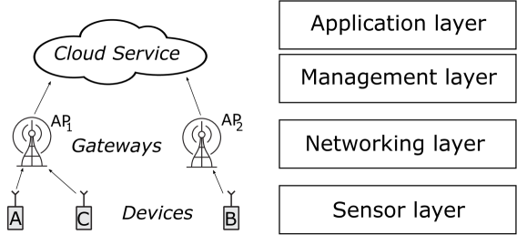
Figure 1: IoT deployment topology and architecture. A gateway could be, for example, a cellular towers, a LPWAN access point, or a satellite. The network topology between devices and gateways may be a mesh or a star-topology. The IoT deployment is connected to a virtual IoT server in the cloud, which manages the network and makes application features available to end users. The different tiers of the network are directly sensing different information about the network. Information regarding link quality of connected devices is available to the APs, but only to the management tier if this information is relayed.

During the past decade, techniques and standards have been developed to provide adequate networking features and improve the Quality of Service (QoS) for the vast number of IoT use cases. An overview of the architecture of IoT services and enabling technologies and protocols is given in [1]. Specifically, in the context of wireless communications, the term IoT usually refers to massive machine-type communication (mMTC), one of the three connectivity types in 5G [2]. Here, a number of pre-5G IoT systems for massive connectivity have been developed and are currently being deployed. These include the low power wide area networks (LPWANs): SigFox, LoRaWAN, NB-IoT and LTE-M [3, 4, 5].

A central problem of wireless IoT connectivity is monitoring and status detection for a massive number of connected devices, which provides insights into the status of the links and devices and can potentially lead to corrective actions  [1, 6, 7]. Network monitoring for wireless sensor networks (WSN) has been researched for decades. A comprehensive survey of network monitoring in wireless sensor networks (WSNs) can be found in [6] and [7]. Arguments for the importance of network monitoring is given by these surveys; network monitoring can enhance data reliability, bandwidth utilization, and the lifetime of the WSN due to the opportunity to identify faulty devices and hence better utilize constrained resources. Multiple monitoring methods can be combined through frameworks, such as fuzzy logic [8] to optimize decision making for fault tolerance. In general, the fault detection methods for WSNs assume a PAN mesh topology such as 6LoWPAN or ZigBee. For example, PAD, a passive monitoring method relying on inference based on routing changes is presented in [9]. Nevertheless, LPWANs are one-hop star-topology networks and additionally, PAD introduces a few bytes of overhead to transmissions, which is a major drawback for energy-constrained devices and networks supporting massive numbers of devices. Notably, the fault detection methods of [10] and [11] rely on statistical inference based on the timing of incoming traffic to detect faults in the network. These methods may readily be modified for and applied to LPWANs since they do not rely on topology changes in a mesh network, but they have the drawback of requiring fault-less training data in order to recognise healthy behavior and the detected errors are only quantifiable at a low resolution, ie. ”no errors, some errors or many errors”.

In this paper, we make no assumption about the topology of the network and instead we assume a quasi-periodic traffic model as that depicted in Fig. 2 for device A and B, which is common for IoT applications. This approach allows us to evaluate the state and link performance of individual devices passively, which is important for identifying poor performers and malfunctioning devices in massive IoT deployments. In our model devices can run ’thin’ clients (a single application) or ’thick’ clients (multiple applications). We have observed the latter behaviour in a data-set from a LoRaWAN deployment, where mains-powered sensors and actuators were used to control and manage street lights in rural towns. We propose parametric machine learning methods for high resolution, centralised and passive fault detection in arbitrary IoT deployments. The methods use temporal correlations in observed traffic to parameterize quasi-periodic applications. The modelled applications are used to infer the state and the QoS of individual devices. Interestingly, the methodological basis for this work has been drawn from research in astronomy, where unevenly sampled time series are common. Astronomers have developed techniques for analyzing such series including phase-folding [12] and a variant of the classical Fourier periodogram that is generalised for uneven time-series [13, 14, 15, 16].

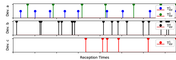
Figure 2: Devices generate traffic depending on their applications. Here the traffic patterns are depicted for three types of devices; Dev. a) runs two applications that generate quasi-periodic traffic. The received traffic streams are shown for both labeled and unlabeled traffic. Dev. b) runs three quasi-periodic applications, but does not label the traffic.

The paper is structured as follows: We introduce our traffic model, the traffic meta-data that can be expected to be available for analysis, and targeted network KPIs in Sec. II. In Sec. III-A we analyze the sub-problem of parametric regression for traffic that is labeled by its parent application. The classification problem of labeling traffic when the traffic parameters are known, but the parent applications are unknown, is examined in Sec. III-B. In Sec. IV we treat the clustering problem that arises when no a priori information is given. Performance results for the algorithms presented throughout can be found in Sec. V and the results of using the fault-detection algorithms on a real-world smart metering deployment can be found in Sec. VI. Sec. VII contains concluding remarks. Table II on page II provides a list of symbols and mathematical notations.

II System Model and Key Performance Indicators

Consider an IoT deployment like that of Fig. 1 & Fig. 2 where sporadically transmitting devices are connected to a server by an arbitrary networking technology, for example an LPWAN, or a mesh network. Here, a virtual server running in the cloud acts as a centralised management layer for network monitoring. The wireless network acts as a filter upon transmitted data introducing intermittency in the form of outage and delays in the received data. In this section we generalise this model to any number of gateways and devices running any number of applications. First, we present the meta-data available in a passive monitoring scenario, define a traffic model for quasi-periodic IoT devices, a set of key performance indicators (KPIs) and a naïve method for evaluating the KPIs. Lastly, we examine how meta-data changes the nature of the machine learning problem.

II-A Available Traffic Meta-Data

In Fig. 1 the devices A and C transmit data through AP₁ while device B transmits data through AP₂. The data that is available for analysis at the server depends on how much meta-data AP₁ and AP₂ relay to the server in addition to how much meta-data is included in the transmissions. When a network is licensed from a network provider then it is considered to be a public network [17]. A network that is closed to the public, privately owned or purpose-built specifically for an IoT deployment, is considered a private network. The same network can be considered private to its owner and public to licencees. In private networks link level metrics, such as received signal strength indicator, link quality indicator, signal to noise ratio, channel state information, modulation and coding rate, are available whereäs they are not necessarily available in public networks. Some network technologies and protocols have specific meta-data built in to the protocol, for example GPS coordinates in SigFox. Such metrics can not always be expected to be available in public networks.

We define a minimal set of metrics that are available in any type of network, {Network ID, Device ID, Reception Timestamp, Payload size}. Device and Network identifiers are a necessary part of a useful transmission. The transmission size and reception time can likewise be found for any transmission. This ensures that the network monitoring is applicable both for network operators, who licence their networks to IoT deployments, but do not have in-depth knowledge of the IoT deployment or access to transmitted data and IoT vendors and operators, who do not have insight into the networking components or access to link-level meta-data.

In addition to this minimal set of metrics, devices may include the ID of their parent application as meta-data within the transmission. This is the behavior of device A in Fig. 2 in contrast to device C, which does not label its traffic. The implication of labeling is that we may pose the fault detection problem as a regression problem instead of a clustering problem. We discuss this implication further in Sec. II-E after defining our traffic model and KPIs.

II-B Traffic model

The traffic generated by a device is the composite of the traffic generated by all the applications running on the device. We denote the number of apps running on a device by $I_{\mathrm{apps}}$. Traffic of one app may influence the jitter of traffic of another app due to queuing of transmissions in the device.

$$T^{x}_{\mathrm{RX}}=T^{1}_{\mathrm{RX}}\cup T^{2}_{\mathrm{RX}}\cup...\cup T^{(i)}_{\mathrm{RX}}\cup...\cup T^{I_{\mathrm{apps}}}_{\mathrm{RX}}$$ (1)

Where $T^{i}_{\mathrm{RX}}=$ {$T^{i}_{1},T^{i}_{2},...,T^{i}_{m},...T^{i}_{M-1},T^{i}_{M}$} denotes the received transmissions from application $i$.
We define Quasi-periodic applications:

These are applications, which send periodic reports, but where the received traffic is intermittent due to queuing and filtering by the network. Common IoT use cases such as gas-, water- and electric smart metering, smart agriculture and smart environment [18, 19], are considered by 3GPP to be quasi-periodic [18].

The $i$th quasi-periodic app generates transmissions at approximately constant intervals, such that the reception times of transmissions from app $i$ can be described by:

$$T^{i}_{{m^{i}}}=\beta^{i}+\alpha^{i}\cdot(m^{i}+o^{i}_{m^{i}})+J^{i}_{m^{i}}$$ (2)

where $\beta^{i}$ is a time offset, $\alpha^{i}$ is the inter-arrival time of app $i$, $J^{i}_{m}$ is a random delay introduced by the network (jitter), $m^{i}$ is the index of the received packets while $o^{i}_{m^{i}}$ is the cumulative number of transmissions that were not received until observation $m^{i}$. Let $n^{i}$ be the index of the transmissions such that $n^{i}=m^{i}+o^{i}_{m^{i}}$. Then we know that $T^{i}_{n-1}\cong T^{i}_{n}\cong T^{i}_{n+1}\pmod{\alpha^{i}}$ for the quasi periodic app $i$.

II-C Key Performance Indicators

We wish to monitor the link quality and status of individual devices in IoT networks. Based on the available meta-data we choose to monitor network outage and online/offline status, which are common KPIs in wireless network performance modelling. In this subsection we define each of these KPIs.

II-C1 Offline detection

An app or a device is considered to be offline if it stops generating transmissions. An intuitive classifier for offline status is detecting whether $k$ consecutive expected transmissions have been missed. This can be done at the application level to classify applications as offline or at the device level, to classify an entire device as offline. Offline applications are not expected to generate transmissions and so they do not count towards the calculated outage. We define a classifier for offline entities, $C_{\text{Off}}$.

$$C_{\text{Off}}:o^{i}(t)\geq k$$ (3)

where $o^{i}(t)=\bigg{\lfloor}\dfrac{t-T^{i}_{m^{i}}}{\alpha^{i}}\bigg{\rfloor}$ computes the expected number of transmissions at time $t$ since the last reception at $T^{i}_{m^{i}}$ if the quasi-periodic app $i$ was online.

II-C2 Outage probability

We define the outage probability as the ratio of the number of packets lost to the number of transmitted packets over a window $\tau_{w}$ at time $t$.

$${p_{\mathrm{o}}^{*}}=\sum_{i=1}^{I_{\mathrm{apps}}}o_{m^{i}(t,\tau_{w})}\Bigg{/}\sum_{i=1}^{I_{\mathrm{apps}}}n^{i}(t,\tau_{w})$$ (4)

where the number of transmitted and received packets for app $i$ from time $t-\tau_{w}$ to $t$ are denoted by $n^{i}(t,\tau_{w})$ and $m^{i}(t,\tau_{w})$, respectively. As $n^{i}(t)$ approaches $\infty$ the observed outage, ${p_{\mathrm{o}}^{*}}$, approaches the network outage probability, ${p_{\mathrm{o}}}$, if ${p_{\mathrm{o}}}$ is stationary over observation period.

$o_{m^{i}(t)}$ and $n^{i}(t)$ are latent variables from the IoT server’s perspective. Then the goal of fault detection can be posed as the problem of estimating these latent variables correctly.

II-D Naïve monitoring method

Here, we introduce a naïve monitoring method, which we will compare other methods to. The approach is straightforward; Denote the number of transmissions received within $\tau_{w}$ at time $t$, $m_{\mathrm{obs}}(t,\tau_{w})$, and let $m_{\mathrm{max}}$ denote the maximum value of $m_{\mathrm{obs}}(t,\tau_{w})$ for $t<t_{now}$. Then we have (5).

$${p_{\mathrm{o}}^{*}}(t,\tau_{w})=\dfrac{m_{\mathrm{max}}-m_{\mathrm{obs}}(t,\tau_{w})}{m_{\mathrm{max}}}$$ (5)

Devices where ${p_{\mathrm{o}}^{*}}(t,\tau_{w})>\epsilon$ are classified as offline.

II-E A priori knowledge and labeled traffic

We may have a priori knowledge about online devices and applications, and we may receive meta-data identifying the app source of traffic. This changes the nature of the fault monitoring problem as depicted in Table I. In the case where we know the parameters of the traffic model and transmissions are labeled (or all clients are ’thin’) it is straightforward to calculate the KPIs. In case the traffic model is unknown, but traffic is labeled we must perform a regression of the traffic parameters in order to calculate the KPIs, which is treated in Sec. III-A. In Sec. III-B we examine the case that traffic parameters are known, but the traffic is unlabeled (and from a ’thick’ client) we must classify received packets as belonging to one app or another to evaluate the KPIs. Finally, we tackle the problem of clustering when the traffic parameters are unknown and the traffic is unlabelled in Sec. IV.

Determining problem		Known applications
nature and applicable		& traffic parameters
methodology		Yes	No
Labelled traffic	Yes	KPI calculation	Regression
	No	Classification	Clustering

TABLE I: Diagram of the classes of the fault detection problem.

III Regression and Classification

III-A Regression

In case transmissions are labeled by their parent application, the composite stream of received packets from all applications can easily be sorted by application such that the stream of any periodic application is on the form of (2). We wish to learn $\alpha^{i}$ and $o^{i}_{m^{i}}$ given a set of reception times, $T^{i}_{\mathrm{RX}}=$ {$T^{i}_{1},T^{i}_{2},...T^{i}_{m}...T^{i}_{M-1},T^{i}_{M}$}. Phase-folding methods like phase dispersion minimization [12] could solve this problem in a brute-force manner by estimating the fit of all potential $\alpha^{i}$, but the associated computational overhead is undesired for massive online network monitoring.

Instead, we propose Normalised Harmonics Mean (NHM), which is an online method we developed for finding an estimate $\alpha^{i*}$ of $\alpha^{i}$ in a set $T^{i}_{\mathrm{RX}}$ with a relatively low amount of computational effort.

Consider a MMSE of the distance between a reception time and transmission time, $\min(|T^{i}_{{n^{i}_{m^{i}}}}-T^{i}_{{m^{i}}}|^{2})$ where $n_{m}^{i}=m^{i}+o_{m^{i}}$. Here $o_{m^{i}}$ and $n_{m^{i}}$ are unknown to the receiver, but we know that the generating function for $T^{i}_{n_{m^{i}}}$ is periodic. We may solve the problem by brute-force using least-squares, however this requires finding $n_{m^{i}}$, which minimizes the MSE for every arrival ${m^{i}}$ for every proposed $\alpha^{i}$, which makes this solution computationally expensive and the accuracy depends on the $\alpha^{i}$ grid chosen for the analysis. This is similar to the brute-force approach of phase dispersion minimization [12].

We propose to use a periodic function, specifically the cosine, to describe the problem. Then we have (6) at the transmitter side and (7) at the receiver side.

$$\cos\Bigg{(}\dfrac{T^{i}_{{n_{m}^{i}}}-T^{i}_{{n_{m}^{i}-1}}}{\alpha^{i}}\cdot 2\pi\Bigg{)}=1$$ (6)

$$\cos\Bigg{(}\dfrac{T^{i}_{{m^{i}}}-T^{i}_{{m^{i}-1}}}{\alpha^{i}}\cdot 2\pi\Bigg{)}>0\quad,\quad 0<J^{i}_{m^{i}}<\dfrac{\alpha^{i}}{2}$$ (7)

So we need to solve for $\alpha^{i}$ that maximizes (7), which may be rephrased as trying to get ${(T^{i}_{{m^{i}}}-T^{i}_{{m^{i}-1}})}/{\alpha^{i}}$ to be as close to an integer as possible.

NHM is based on this observation and attempts to find $\alpha^{i}$ in a gradient-descent manner, by searching for the set of best fitting integers to normalise the distances between elements in $T^{i}_{\mathrm{RX}}$. The step-wise procedure of NHM is described by Alg. 1.

Data: $dT^{i}_{\mathrm{RX}}$

Result: $\alpha^{i*}$

1 Make a preliminary hypothesis for $\alpha^{i*}$.

2 while $\alpha^{i*}$ has not converged do

3       Estimate $\eta^{i}_{m^{i}}$ for $\alpha^{i*}$.

4       Update the hypothesis for $\alpha^{i*}$ based on $\eta^{i}_{m^{i}}$.

Calculate KPIs based on app parameters.

Algorithm 1 Normalised Harmonics Mean (NHM)

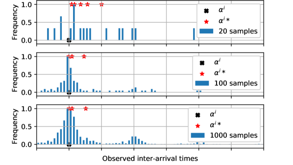
Figure 3: Histogram of $dT^{i}_{\mathrm{RX}}$ where $J^{i}_{m}~{}\sim~{}\exp(.25)\cdot{\alpha^{i}}{/2}$ and ${p_{\mathrm{o}}}=0.2$. The red crosses indicate the iterations of $\alpha^{i*}$ in NHM, which can be seen to approach $\alpha^{i}$, even when few samples are available. In this example, the initial hypothesis of $\alpha^{i*}$ was based on the mean of $dT^{i}_{\mathrm{RX}}$.

Let the set $dT^{i}_{\mathrm{RX}}$ denote the set of the distances between neighboring elements $T^{i}_{\mathrm{RX}}$. The preliminary hypothesis for $\alpha^{i}$ could be $\alpha^{i*}=\mathrm{mean}(dT^{i}_{\mathrm{RX}})$.

Outage creates harmonic contributions of orders higher than 1, $o^{i}_{m^{i}}>0$, in the set $dT^{i}_{\mathrm{RX}}$ as depicted in Fig. 3. In the next step we seek to normalize these harmonics by estimating the series of latent variables $\eta^{i}_{m^{i}}$ given by (8). We do this under the condition that $||J||<\dfrac{\alpha^{i}}{4}$ (or equivalently $0\leq J<\dfrac{\alpha^{i}}{2}$) such that aliasing is avoided, $n^{i}_{m^{i}}\leq n^{i}_{m^{i}+1}+1$, which in practice means that a transmission is never received earlier than a previous transmission.

$$\eta^{i}_{m^{i}}=\bigg{\lfloor}\dfrac{T^{i}_{m^{i}}-T^{i}_{m^{i}-1}}{\alpha^{i*}}\bigg{\rceil}$$ (8)

where $n^{i}_{m^{i}}=\sum_{k=1}^{{m^{i}}}\eta^{i}_{k}\quad\Leftrightarrow\quad\eta^{i}_{m}=n^{i}_{m}-n^{i}_{m-1}$.

The initial hypothesis for $\alpha^{i*}$ is unlikely to be correct, but it serves to provide an initial estimate of the latent series $\eta^{i}_{m^{i}}$, which we can now use to estimate $\alpha^{i}$. Given the hypothesis that $\alpha^{i}$ is the mean of a normalised version of $dT^{i}_{\mathrm{RX}}$ we have (9).

$$\alpha^{i*}=\dfrac{1}{M^{i}}\sum_{m^{i}=2}^{M^{i}}{\bigg{(}\dfrac{T^{i}_{m^{i}}-T^{i}_{m^{i}-1}}{\eta^{i}_{m^{i}}}\bigg{)}}$$ (9)

Iterative updates of $\eta^{i}_{m^{i}}$ and $\alpha^{i*}$ Eq. (9) will gradually go towards $\alpha^{i}$ as depicted in Fig. 3. The required number of iterations for convergence depends on the accuracy of the initial estimate of $\alpha^{i}$, which is dependent on ${p_{\mathrm{o}}}$ and the number of samples. After the algorithm convergences the estimated number of transmissions lost between successive receptions is given by the latent variables $o^{i}_{m^{i}}=n^{i}_{m^{i}}-n^{i}_{m^{i}-1}$. Furthermore $\beta^{i}$ can be found by linear regression of (2) as both $\alpha^{i}$ and $n^{i}_{m^{i}}$ have been estimated, but is not necessary for computing the KPIs in our case.

NHM can be run in an online manner by saving $dT^{i}_{\mathrm{RX}}$ and $T^{i}_{M+1}$ and updating both upon reception of a new transmission for app i before repeating step 2 starting from the previous $\alpha^{i*}$.

III-B Classification

In case the parameters $\alpha^{i}$ and $\beta^{i}$ are known for all applications $i\in I$, but transmissions are not labeled by their parent application, we need to classify which application a new reception belongs to. Let $f(T^{i}_{\mathrm{RX}},\alpha^{i},\beta^{i})$ be the transmission generating function, then we may propose a periodic likelihood function $g(T^{i}_{\mathrm{RX}},\alpha^{i},\beta^{i})$, such that

$$f(T^{i}_{\mathrm{RX}},\alpha^{i},\beta^{i})\propto g(T^{i}_{\mathrm{RX}},\alpha^{i},\beta^{i})=\dfrac{\cos\bigg{(}\dfrac{T^{i}_{\mathrm{RX}}-\beta^{i}}{\alpha^{i}}\cdot 2\pi\bigg{)}+1}{2}$$ (10)

Then $i$ is found by $\max_{i∈\{1:I_{\mathrm{apps}}\}}(g(T^{i}_{\mathrm{RX}},\alpha^{i},\beta^{i}))$. Here, we chose a cosine function as a likelihood function and added 1 before normalizing to keep the probability between 0 and 1. In practice the maximization yields the same result regardless of these linear operations due to the associative property of the periodic likelihood function.

A sub-problem here is the initial classification when $\beta^{i}$ is not known, while $\alpha^{i}$ is known, we must find the most likely sequence of packets to belong to the process that has the inter-arrival time $\alpha^{i}$ for some $\beta^{i}$. Then $g(T^{i}_{a}-T^{i}_{b},\alpha^{i},\beta^{i}=0)$ is the likelihood that transmissions $a$ and $b$ belong to the same sequence with inter-arrival time $\alpha^{i}$. If we then let transmission $m$ be a newly received packet and $m^{i}$ be the last packet received by app $i$, then we can simply find $i$ by $\max_{i∈\{1:I_{\mathrm{apps}}\}}(g(T^{i}_{m}-T^{i}_{m^{i}},\alpha^{i},\beta^{i}=0))$. Notice, that errors in the estimate of $\alpha$ will results in a error in the output of $g$, which increases as the distance between two timestamps increases, or in other words, labeling is more likely to be erroneous as ${p_{\mathrm{o}}}$ increases or after offline periods.

IV Clustering

When traffic parameters are unknown and the traffic is unlabeled by its parent application we need to perform clustering of the received traffic. In this section we propose a clustering algorithm that estimates clusters in a hierarchical manner based on the Lomb-Scargle periodogram and an online version, which assigns newly received transmissions to already known clusters in a greedy manner.

Let the set of all unassigned traffic received by device $x$ be $T^{x*}_{\mathrm{RX}}$.The procedure for the hierarchical clustering method, Successive Periodicity Clustering (SPC) is described in Alg. 2.

Data: $T^{x}_{\mathrm{RX}}$

Result: {$T^{i*}_{\mathrm{RX}}$, $\alpha^{i*}$ , $\beta^{i*}$ }, $T^{i}_{\mathrm{RX}}\in T^{x}_{\mathrm{RX}}$

1 while  do

2       Hypothesize $\alpha^{i*}$ for an app $i$, given $T^{x*}_{\mathrm{RX}}$.

3       if $\alpha^{i*}$ is significant then

4             Label data points that best fit $\alpha^{i*}$ and extract $\beta^{i*}$ and $T^{i*}_{\mathrm{RX}}$.

5             Calculate KPIs based on $\alpha^{i*}$, $\beta^{i*}$ and $T^{i*}_{\mathrm{RX}}$.

6             Remove $T^{i*}_{\mathrm{RX}}$ from the set of unlabeled data. $T^{x*}_{\mathrm{RX}}=T^{x*}_{\mathrm{RX}}\text{\textbackslash}T^{i*}_{\mathrm{RX}}$

7      else

8             return {$T^{i*}_{\mathrm{RX}}$, $\alpha^{i*}$ , $\beta^{i*}$ }, $T^{i}_{\mathrm{RX}}\in T^{x}_{\mathrm{RX}}$

9      

Algorithm 2 Successive Periodicity Clustering (SPC)

NHM can be used for creating a hypothesis for $\alpha^{i}$. This is a robust approach as long as $\alpha^{1}<<\alpha^{2}<<...<<\alpha^{I_{\mathrm{apps}}}$ with an estimation error that increases greatly as $\dfrac{\alpha^{i}}{\alpha^{i+1}}\to 1$. However, it may often be the case that $\dfrac{\alpha^{i}}{\alpha^{i+1}}\approx 1$ so we will examine using the Lomb-Scargle periodogram for hypothesis creation instead.

Lomb in [13] proposed a least-squares periodogram, which tested for the best fitting set of frequencies for a unevenly sampled time-series. In [14], Scargle proposed a generalised form of the classical Fourrier periodogram, which turns out to be equivalent to the least-squares fitting of sinusoids from [13]. Hence, this periodogram was termed Lomb-Scargle periodogram and [15] treats its statistical properties, including a close-upper limit on the probability of falsely detecting a peak frequency in a data set comprised solely of noise. The Lomb-Scargle periodogram is well-known in some scientific communities, but was recently introduced to a wider audience in [16] by surveying works on and related to the Lomb-Scargle periodogram and lending conceptual intuitions. The Lomb-Scargle algorithm has been implemented in Python in the Astropy package [21, 22].

IV-A Lomb-Scargle-based hypothesis creation for $\alpha$

The classical Fourier periodogram requires evenly sampled data, but the Lomb-Scargle algorithm can find a PSD-like density for unevenly spaced times series [13, 14, 16].

Preprocessing of our data is required. We generate a series $V$ which is the same size as $T^{x*}_{\mathrm{RX}}$ and holds the value 1 for each of the timestamps. Then we interpolate $V$ with 0’s to permit sine-based analysis. We carry out this interpolation in a heuristic manner by finding places in $dT^{x*}_{\mathrm{RX}}$ larger than $dT^{x*}_{\mathrm{RX}}$ in an attempt to avoid interpolation between transmissions that are very close in time, i.e., to avoid giving credibility to very high frequencies.

We must identify the frequency spectrum that is relevant for analysis. The size of the set of frequencies within the grid dictates both accuracy and computational effort, since ’false positive’ local peaks in the periodogram are less likely to be found to be the global peak, but at the expense of evaluating the periodogram in more points. The minimum detectable frequency will be a signal that completes one oscillation over the entire period of the data-set, $f_{\text{min}}=\dfrac{1}{T^{x*}_{M^{x*}}-T^{x*}_{1}}$. The spacing of the frequency grid, $\delta f=\dfrac{1}{n_{0}\tau_{\text{w}}}$, depends on an oversampling factor, $n_{0}$. The higher $n_{0}$ is, the higher the chance that a peak frequency is not missed in the analysis. Typically, 8 is used [16]. The Nyquist limit does not always exist for the unevenly sampled Lomb-Scargle periodogram and in our case it will inevitably be very large since $f_{Ny}=1/(2p)$, where $p$ is the largest value that all $T^{x*}_{\mathrm{RX}}$ can be written as an integer multiple of [23]. Instead we shall use a heuristic to determine $f_{\max}$. Say that $I_{\mathrm{apps}}$ applications are generating packets with rates $\alpha^{i}$ and there is no outage. In this case the mean observed inter-arrival time is always less than or equal to $\dfrac{1}{M^{i}-1}\sum_{{m^{i}}=1}^{M^{i}-1}(dT^{i}_{{m^{i}}})\leq\min_{i\in\{1:I_{\mathrm{apps}}\}}(\alpha^{i})$. Then if we choose $f_{\max}$ such that

$$f_{\max}=\dfrac{L}{\dfrac{1}{M^{x*}-1}\sum_{{m^{x*}}=1}^{M^{x*}-1}(dT^{x*}_{{m^{x*}}})}$$ (11)

where L is scalar used to take into account the effect of outage. Given 50% outage in a set of times one would expect to find a mean inter-arrival time that is twice as long. So assuming L = 2, our heuristic limit for the frequency grid should cover the maximum frequency of any observed app for ${p_{\mathrm{o}}}\leq 50\%$.

Let $Z=P(f)$ be the periodogram value at frequency $f$. In [14] it was observed that the probability of observing a periodogram value less than Z in pure Gaussian noise can be expressed as (12).

$$P_{\mathrm{single}}(Z)=1-\exp{(-Z)}$$ (12)

A close-upper limit for the false alarm probability, $\mathrm{FAP}(Z)$, was found by Baluev in [15]. We access this limit at the peak-value of the periodogram, $Z_{0}$, with significance, $\sigma$ and only accept the hypothesis $\alpha^{*}=1/f_{0}$ if $\mathrm{FAP}(Z)<\sigma$.

IV-B Labeling and collision resolution

If a significant peak is detected we need to label data that fits the suggested $\alpha^{i*}$. Since up to $I_{\mathrm{apps}}$ apps have generated $T^{x}_{\mathrm{RX}}$ we must attempt to find the sequence of data points that is the best fit for our proposed application $i$. We do this by labeling transmissions, which fit coarsely and then sorting out incoherent false positive transmissions. Given a significant proposal for $\alpha^{i*}$ the procedure is:

1. Mark transmissions that seem to be a good fit for $\alpha^{i*}$.

2. Remove marks from transmissions that are incoherent with the rest of the labeled transmissions.

3. Label marked transmissions as belonging to app $i$.

4. Calculate KPIs based on app parameters and labeled packets.

We calculate the fit between all times in all possible sequences by building a matrix $\textbf{IA}=\textbf{T}^{\textbf{x*}}_{\mathrm{\textbf{RX}}}\textbf{U}-\textbf{T}^{\textbf{x*}}_{\mathrm{\textbf{RX}}}\textbf{U}^{T}$ where U is a vector of ones [1,1,1,…,1] of length $M$ and $\textbf{T}^{\textbf{x*}}_{\mathrm{\textbf{RX}}}$ is a vectorized version of the set of unlabeled transmissions. We then proceed to estimate the fit, $\phi_{m}$, of each transmission to all other transmissions given $\alpha^{i*}$ as (13).

$$\phi_{m}=\sum_{n=1}^{M}\big{(}g(\textbf{IA}_{(m,n)},\alpha^{i*},\beta^{i}=0)\big{)}$$ (13)

Now, a preliminary sorting of transmissions is performed by labeling only transmissions for which $\phi_{m}~{}>~{}\dfrac{1}{2M^{x*}}\sum_{m=1}^{M^{x*}}(\phi_{m})$. This coarse sorting of packets results in a fair amount of false positives in $T^{i*}_{\mathrm{RX}}$. False positives can in many cases (especially when ${p_{\mathrm{o}}}$ is low) be identified as clearly incoherent transmissions that ’collide’ in time with other transmissions in the set. The minimal period between packets is $\dfrac{\alpha^{i*}}{2}$ before a pair of transmissions are considered to collide. This is conditioned by $||J^{i}||<\dfrac{\alpha^{i*}}{4}$. Colliding pairs are resolved by checking the fit of the colliding packets and removing the worst fitting transmission from the set of transmissions for the new app. Given a collision at $T^{x}_{l}$ and $T^{x}_{l+1}$ we have that

$$C_{l\in\{1:M^{i}\}|app^{i}}:\phi_{l}>\phi_{l+1}$$ (14)

Now we have estimated $T^{i}_{\mathrm{RX}}$ from the set of unlabeled data. Since the Lomb-Scargle method is only as accurate as the frequency grid we use in its analysis, we can attempt to use NHM on the estimated set $T^{i}_{\mathrm{RX}}$, to get better estimate for $\alpha^{i}$. Then we can compute KPIs for the application and finally remove the labeled traffic from $T^{x*}_{\mathrm{RX}}$ and attempt SPC again.

IV-C Greedy online clustering

SPC does batch processing and is relatively computationally heavy. An online version of the algorithm that minimizes the computational effort and can be used for real-time monitoring is warranted. So we introduce a greedy online clustering (GOC) algorithm. Upon the reception of a new transmission $T^{x}_{M^{X}}$ GOC runs as described in Alg. 3.

Data: $T^{x}_{M^{X}}$,{$T^{i*}_{\mathrm{RX}}$, $\alpha^{i*}$ , $\beta^{i*}$ }, $T^{i}_{\mathrm{RX}}\in T^{x}_{\mathrm{RX}}$

Result: {$T^{i*}_{\mathrm{RX}}$, $\alpha^{i*}$ , $\beta^{i*}$ }, $T^{i}_{\mathrm{RX}}\in T^{x}_{\mathrm{RX}}$

1 Estimate the fit $\phi^{i*}$ of the new arrival $T^{x}_{M^{X}}$ for every previously known app $i$.

2 if $\max(\phi^{i})>0$ then

3       Add the transmission $T^{x}_{M^{X}}$ to the app $j$ which had the best fit.

4       Update the parameters, $\alpha^{i*}$ , $\beta^{i*}$.and the KPIs for $i$.

5else

6       Add the transmission to the set of unlabeled transmissions $T^{x*}_{\mathrm{RX}}$. and run SPC on $T^{x*}_{\mathrm{RX}}$.

Algorithm 3 Greedy Online Clustering (GOC)

Once a new transmission is received, it should be checked if the reception time fits with the expected reception time of any known applications. GOC estimates $\phi^{i}~{}=~{}g(T^{x}_{M^{X}}~{}-~{}T^{i}_{M^{i}},\alpha^{i*},\beta^{i}~{}=~{}0)$ for all known $i$. Then assigns the transmission to $T^{i}_{\mathrm{RX}}$ if $\max_{i\in\{1:I_{\mathrm{apps}}\}}(\phi^{i})$ is positive. Then the KPIs are updated for app $i$.

In case $\max_{i\in\{1:I_{\mathrm{apps}}\}}(\phi^{i})\leq 0$ the new transmission is added to the set of unlabeled transmissions $T^{x*}_{\mathrm{RX}}$ and SPC is attempted.

V Probabilistic Performance

In this section numerical results for the performance of the algorithms introduced throughout this paper are presented. The performance is evaluated in terms of the accuracy of the outage estimation and offline state detection.

All the presented algorithms and the naïve method presented in Sec. II-D have been implemented in Python. The implementations are based on functionality from the Numpy package [24] and the Lomb-Scargle algorithm of the Astropy package [21, 22]. A parameter $\psi$ that reduces the computational requirements and enhances the accuracy of SPC and GOC has been introduced. $\psi$ ensures that SPC is only ever run when $T^{x*}_{\mathrm{RX}}$ is larger than $\psi$. Furthermore after labeling and collision resolution the size of the proposed set $T^{i}_{\mathrm{RX}}$ is checked and only accepted if it is larger than $\psi$.

The performance has been evaluated against network outage probabilities, ${p_{\mathrm{o}}}=[0,.1,.2,.3,.5]$. For each data point 1000 stochastic transmission sequences with jitter and outage have been generated. Outage has been randomly induced in the sequences by generating samples for $T^{i}_{\mathrm{RX}}$ and discarding $T^{i}_{\mathrm{m}^{i}}$ with probability ${p_{\mathrm{o}}}$ until the specified sample size was reached. Sample sizes of 5, 10, 25, 50 and 100 transmissions have been used. The traffic parameters are drawn from the following distributions:

$$\alpha^{1}\sim U(100,200)$$

$$\alpha^{2}\sim U(1,5)\cdot\alpha^{1}$$

$$\beta^{i}\sim U(0,0.5)\cdot\alpha^{i}$$

$$j^{i}_{m}\sim\exp(0.2)\cdot\dfrac{\alpha^{i}}{20}$$

V-A Network outage detection and estimation

The absolute estimation error, $|{p_{\mathrm{o}}}-{p_{\mathrm{o}}^{*}}|$, is plotted in Fig. 4 for NHM and the naïve method on a labelled sequence and SPC, GOC and the naïve method for unlabelled sequences. The labelled sequence is $T^{1}_{\mathrm{RX}}$, and the unlabelled sequence is $T^{x}_{\mathrm{RX}}=T^{1}_{\mathrm{RX}}\cup T^{2}_{\mathrm{RX}}$ and $\psi=\min(s_{\min},25)$ for SPC and GOC, where $s_{\min}=\min(M^{1},M^{2})$.

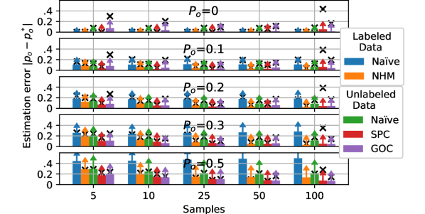
Figure 4: Absolute error in network outage estimation for NHM, GOC, SPC and the naïve approach. The naïve method is applied to both the labeled data-set and the unlabeled data-set ($\tau_{w}=1500$). The bars indicate the mean absolute errors, the arrows indicate the size of the standard deviation and the 95th percentile is denoted by the black crosses.

The naïve approach works well when there is little to no uncertainty, but both the mean error and the variation in error increases rapidly as ${p_{\mathrm{o}}}$ increases. Notice that NHM has both a lower mean and less variance in the estimation error, especially as the number of available samples increase. Indeed, NHM has a $<$5% estimation error at ${p_{\mathrm{o}}}=0.3$ for 50 available samples. On unlabeled data-sets, The naïve approach is found to perform a little better, which is expected due to the increased number of samples within the ’windowing’ function of the naïve approach. Still, both SPC and GOC outperforms the naïve approach as ${p_{\mathrm{o}}}$ increases. We observe that SPC performs a little worse at 100 samples compared to 50 samples - this can be explained by the periodic labelling function performing worse over such a long period of samples, which is exaggerated when SPC then tries to find an ’imaginary’ application to label transmissions that should have been assigned previously. In GOC, the inaccuracy of the periodic labelling function causes errors when only a few samples are available, here ’false positive’ labels result in the secondary application not finding sufficient samples to satisfy $\psi$.

V-B Offline state detection

In this scenario the device goes offline and we denote the number of transmissions since the device went offline, $o_{M}^{x}$. We define the false alarm probability (FAP) as the probability that an offline state is detected when the device is not offline. In Fig. 5 the resulting probabilities are plotted. We observe that GOC identifies devices as offline correctly with a high probability. The probability of correctly identifying offline devices increases with the number of sampled reception times. The FAP for GOC increases with the network outage, as $\alpha^{i*}$ is more prone to be inaccurate, which is also the case when a very small number of samples are available before the device goes offline. Furthermore, when the network outage is high, the device is more likely to appear offline due to random outage in the received sequence $T^{x}_{RX}$, which affects the naïve method significantly more than GOC.

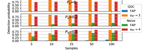
Figure 5: Probabilities of detecting offline-state in different conditions for the real-time clustering method, GOC, and the naïve approach ($\epsilon=.25$, $\tau_{w}=1500$). FAP denotes the false alarm probability. $o_{M^{x}}$ denotes the number of consecutively missed transmissions during the offline period.

V-C Sampling and Computation time

The total computation time of each algorithm is plotted in Fig. 6. The computation time of GOC is significantly larger than that of SPC, since GOC will attempt SPC multiple times as transmissions are received, however, one should note that the cmputing time of GOC when receiving transmissions from known apps is very low, near that of NHM. The computation time of NHM is significantly lower than that of any other method. The naïve approach beats both clustering methods in terms of computation time. Still, in the special case that $\min(\alpha^{i})$ is 1 hour for a group of devices, GOC supports initial analysis of up to 12240 devices in serial on a single thread of a 4.00 GHz i7-6700 if 100 samples are received as batch for each device, but processed in an online manner using GOC (worst-case). In practice, the sampling time for MAR-P traffic [18] would be much greater, such that even more devices could be supported.

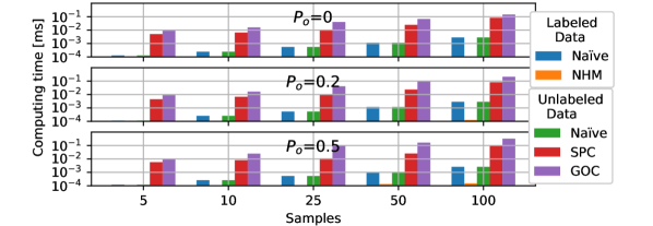
Figure 6: Mean computation time for NHM, SPC, GOC and the naïve approach. Mind that the y-axis is logarithmic.

VI Case study: smart metering deployment

This section presents monitoring results from using GOC on a data-set from a real-world wireless smart metering deployment. The data consists of timestamps, device IDs and IDs of the receiving concentrators for a total of 1048576 received transmissions from 4522 smart meters. The smart meters are deployed in a large area with 6 concentrators that provide coverage for all meters. Meters are connected to concentrators in a star-topology.

Meters broadcast quasi-periodically to the concentrators at an inter-arrival time that is normally distributed around three hours. It should be noted that meters, which do not receive an acknowledgement will include the data of any missed transmissions in their broadcast. Effectively this means that the app layer QoS is kept high even in poor link level conditions. Here, we monitor the network performance at the link level from the perspective of individual concentrators and the perspective of a centralised service gathering data from all concentrators.

The distribution of estimated $\alpha^{i*}$’s using GOC and NHM are plotted in Fig. 7 for the perspective of a central server and as a joint distribution for all concentrators. Here we find that the estimated $\alpha^{*}i$’s are normally distributed around 3 hours for GOC, which is coherent with the deployment case. NHM on the other hand shows a fat tail in the distribution, which is not coherent with our prior knowledge of the transmission rate distribution. This inconsistency can be ascribed to the number of available data, noise in the data and the inaccuracy of NHM at increasingly higher network outages as seen in Fig. 4.

Figure 7: Distributions of estimated inter-arrival times from the perspectives of each concentrator and a centralised server.

Overlapping concentrator coverage enhances the application level-performance; Using GOC, we find that 20.3% of the meters are connected to at-least one concentrator without outage at the link-level, while the same measure is 54.8% from the perspective of a centralised server. The PDF of estimated outages for all meters from the perspective of the concentrators and the centralised server can be found in Fig. 8. Each given device is not necessarily in the range of each deployed concentrator, such that, as expected, we see varying connectivity levels for the different concentrators. The estimated outage at the link level as seen by the server is much lower than that of any individual concentrator. We have used a parameter of $\psi$ = 10 for the analysis. This means that 3.4% of the devices represented in the data were not analysed due to being sampled less than 10 times while another 1.1% did not exhibit clear periodicity due to having few samples and likely a relatively high outage. This group of devices are clear outliers in the deployment and warrant further investigation.

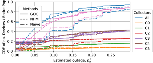
Figure 8: CDFs of estimated outages for each device as seen by each concentrator and a centralised server. The CDFs are evaluated against the entire population of devices in the deployment.

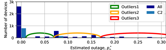
Figure 9: Histogram of estimated outages for devices in the deployment at the central server and concentrator C2. Devices can be grouped in spectra, which increase in width in proportion to the estimated outage, or equivalently, as reliability of the estimate goes down.

The distribution of the estimated outage by NHM and GOC converges after $p_{0}^{*}=5\%$. Both methods identify roughly the same sets of devices for different groups of outliers. The naïve method continually overshoots it’s outage estimation. In Fig. 9 we take a closer look at the links experienced by the concentrator ”C2” and the links as experienced by the server. Here a histogram of the estimated outage at the link-level is depicted. In this way groups of outliers can be identified both at the application level and at the level of individual concentrators. In summary, the methods can quantify the coverage of concentrators in practice, which enables evaluation of their placement. The locations of concentrators and devices would be known by the smart metering company, making it relatively easy to assess spatial correlation of poorly performing devices. Installing a local concentrator is sensible in areas with many poorly performing devices, whereas antenna upgrades might be more cost beneficial for solitary, poorly performing devices. The methods can also help identifying Byzantine transmissions and seasonality in the outage.

VII Conclusion

In this paper we introduced methods for passive detection in IoT networks in deployments with quasi-periodic reporting, such as smart-metering, environmental monitoring and agricultural monitoring. The methods are applicable in both mesh networks and LPWA and cellular networks, setting them apart from the state-of-art methods for fault detection in WSNs.

The SPC and GOC algorithms were shown to perform well even at high outage for composite sequences, which makes them well suited for monitoring devices and networks in ’black-box’ networks where the outage may be quite high. The cost of the utility and precision of these methods is computational effort, which was measured for a 4.0GHz i7-6700 CPU. Furthermore, the utility of NHM and GOC has been exhibited through a short analysis of real-world data from a smart meter deployment.

References

- [1] A. Al-Fuqaha, M. Guizani, M. Mohammadi, M. Aledhari, and M. Ayyash, “Internet of things: A survey on enabling technologies, protocols, and applications,” IEEE Communications Surveys Tutorials, vol. 17, no. 4, pp. 2347–2376, Fourthquarter 2015.
- [2] S. Parkvall, E. Dahlman, A. Furuskar, and M. Frenne, “Nr: The new 5g radio access technology,” IEEE Communications Standards Magazine, vol. 1, no. 4, pp. 24–30, Dec 2017.
- [3] K. Mekki, E. Bajic, F. Chaxel, and F. Meyer, “A comparative study of lpwan technologies for large-scale iot deployment,” ICT Express, vol. 5, no. 1, pp. 1–7, 2019.
- [4] S. Popli, R. K. Jha, and S. Jain, “A survey on energy efficient narrowband internet of things (nbiot): Architecture, application and challenges,” IEEE Access, vol. 7, pp. 16 739–16 776, 2019.
- [5] R. Ratasuk, N. Mangalvedhe, D. Bhatoolaul, and A. Ghosh, “Lte-m evolution towards 5g massive mtc,” in 2017 IEEE Globecom Workshops (GC Wkshps), Dec 2017, pp. 1–6.
- [6] A. Mahapatro and P. M. Khilar, “Fault diagnosis in wireless sensor networks: A survey,” IEEE Communications Surveys Tutorials, vol. 15, no. 4, pp. 2000–2026, Fourth 2013.
- [7] Z. Zhang, A. Mehmood, L. Shu, Z. Huo, Y. Zhang, and M. Mukherjee, “A survey on fault diagnosis in wireless sensor networks,” IEEE Access, vol. 6, pp. 11 349–11 364, 2018.
- [8] M. Nazari Cheraghlou, A. Khadem-Zadeh, and M. a. Haghparast, “A framework for optimal fault tolerance protocol selection using fuzzy logic oniot sensor layer,” International Journal of Information & Communication Technology Research, vol. 10, no. 2, 2018. [Online]. Available: http://ijict.itrc.ac.ir/article-1-326-en.html
- [9] Y. Liu, K. Liu, and M. Li, “Passive diagnosis for wireless sensor networks,” IEEE/ACM Transactions on Networking, vol. 18, no. 4, pp. 1132–1144, Aug 2010.
- [10] B. C. Lau, E. W. Ma, and T. W. Chow, “Probabilistic fault detector for wireless sensor network,” Expert Systems with Applications, vol. 41, no. 8, pp. 3703 – 3711, 2014. [Online]. Available: http://www.sciencedirect.com/science/article/pii/S0957417413009548
- [11] X. Jin, T. W. S. Chow, Y. Sun, J. Shan, and B. C. P. Lau, “Kuiper test and autoregressive model-based approach for wireless sensor network fault diagnosis,” Wireless Networks, vol. 21, no. 3, pp. 829–839, Apr 2015. [Online]. Available: https://doi.org/10.1007/s11276-014-0820-0
- [12] R. F. Stellingwerf, “Period determination using phase dispersion minimization.” Astrophysical Journal, vol. 224, pp. 953–960, Sep 1978.
- [13] N. R. Lomb, “Least-squares frequency analysis of unequally spaced data,” Astrophysics and Space Science, vol. 39, no. 2, pp. 447–462, Feb 1976.
- [14] J. Scargle, “Studies in astronomical time series analysis. ii - statistical aspects of spectral analysis of unevenly spaced data,” The Astrophysical Journal, vol. 263, 01 1983.
- [15] R. V. Baluev, “Assessing the statistical significance of periodogram peaks,” Monthly Notices of the Royal Astronomical Society, vol. 385, no. 3, pp. 1279–1285, April 2008.
- [16] J. T. VanderPlas, “Understanding the lomb–scargle periodogram,” The Astrophysical Journal Supplement Series, vol. 236, no. 1, p. 16, may 2018.
- [17] O. Al-Khatib, W. Hardjawana, and B. Vucetic, “Traffic modeling and optimization in public and private wireless access networks for smart grids,” IEEE Transactions on Smart Grid, vol. 5, no. 4, pp. 1949–1960, July 2014.
- [18] 3GPPP, “Cellular system support for ultra-low complexity and low throughput internet of things (ciot),” 3GPP, Technical report (TR) 45.820, 12 2015, version 13.1.0.
- [19] A. Zanella, N. Bui, A. Castellani, L. Vangelista, and M. Zorzi, “Internet of things for smart cities,” IEEE Internet of Things Journal, vol. 1, no. 1, pp. 22–32, Feb 2014.
- [20] M. Laner, P. Svoboda, N. Nikaein, and M. Rupp, “Traffic models for machine type communications,” in ISWCS 2013; The Tenth International Symposium on Wireless Communication Systems, Aug 2013, pp. 1–5.
- [21] Astropy Collaboration and T. P. e. a. Robitaille, “Astropy: A community Python package for astronomy,” Astronomy and Astrophysics, vol. 558, p. A33, Oct. 2013.
- [22] Astropy Contributers and A. M. e. a. Price-Whelan, “The Astropy Project: Building an Open-science Project and Status of the v2.0 Core Package,” Astronomical Journal, vol. 156, p. 123, Sep. 2018.
- [23] L. Eyer and P. Bartholdi, “Variable stars: Which Nyquist frequency?” Astronomy and Astrophysics, Supplement, vol. 135, pp. 1–3, Feb. 1999.
- [24] T. E. Oliphant, A guide to NumPy. Trelgol Publishing USA, 2006, vol. 1.