Towards $\bar{B}\to X_{s}\gamma$ at the NNLO in QCD without interpolation in $m_{c}$

Abstract

Strengthening constraints on new physics from the $\bar{B}\to X_{s}\gamma$ branching ratio requires improving accuracy in the measurements and the Standard Model predictions. To match the expected Belle-II accuracy, Next-to-Next-to-Leading Order (NNLO) QCD corrections must be calculated without the so-far employed interpolation in the charm-quark mass $m_{c}$. In the process of evaluating such corrections at the physical value of $m_{c}$, we have finalized the part coming from diagrams with closed fermion loops on the gluon lines that contribute to the interference of the current-current and photonic dipole operators. We confirm several published results for corrections of this type, and supplement them with a previously uncalculated piece. Taking into account the recently improved estimates of non-perturbative contributions, we find ${\mathcal{B}}_{s\gamma}=(3.40\pm 0.17)\times 10^{-4}$  and  $R_{\gamma}\equiv{\mathcal{B}}_{(s+d)\gamma}/{\mathcal{B}}_{c\ell\bar{\nu}}=(3.35\pm 0.16)\times 10^{-3}$  for  $E_{\gamma}>1.6\,$GeV in the decaying meson rest frame.

1 Introduction

Flavour Changing Neutral Current (FCNC) processes receive the leading Standard Model (SM) contributions from one-loop diagrams only, often with additional suppression factors originating from the Glashow-Iliopoulos-Maiani (GIM) mechanism Glashow:1970gm . It makes them sensitive to possible existence of new weakly-interacting particles with masses ranging up to ${\mathcal{O}}(100\,{\rm TeV})$. Significant deviations from the SM predictions are observed in the GIM-unsuppressed FCNC processes mediated by the $b\to s\mu^{+}\mu^{-}$ transition (see, e.g., the recent summary in Ref. Aebischer:2019mlg ). On the other hand, no deviations are seen in the closely related $b\to s\gamma$ transition, despite higher accuracy of both the measurements and the SM predictions in its case.

The physical observable giving the strongest constraints on the $b\to s\gamma$ amplitude is the inclusive ${\mathcal{B}}_{s\gamma}$ branching ratio, i.e. the CP- and isospin- averaged branching ratio of $\bar{B}\to X_{s}\gamma$ and $B\to X_{\bar{s}}\gamma$ decays, with $\bar{B}$ and $B$ denoting ($\bar{B}^{0}$ or $B^{-}$) and ($B^{0}$ or $B^{+}$), respectively. The states $X_{s}$ and $X_{\bar{s}}$ are assumed to contain no charmed hadrons. ${\mathcal{B}}_{s\gamma}$ is being measured Chen:2001fja ; Aubert:2007my ; Lees:2012wg ; Lees:2012ym ; Saito:2014das ; Belle:2016ufb with $E_{\gamma}>E_{0}$ for $E_{0}\in[1.7,2.0]$ GeV, and then extrapolated to the conventionally chosen value of $E_{0}=1.6\,$GeV to compare with the theoretical predictions (that would be less accurate at higher $E_{0}$). The current experimental world average for ${\mathcal{B}}_{s\gamma}$ at $E_{0}=1.6\,$GeV reads $(3.32\pm 0.15)\times 10^{-4}$ Amhis:2019ckw , which corresponds to an uncertainty of around $\pm 4.5\%$. With the full Belle-II dataset, the world average uncertainty at the level of $\pm 2.6\%$ is expected Kou:2018nap ; Ishikawa:2019Lyon . Achieving a similar accuracy in the SM predictions is essential for improving the power of ${\mathcal{B}}_{s\gamma}$ as a constraint on Beyond-SM (BSM) theories. It is the goal of the calculations we describe in what follows.

The SM prediction for ${\mathcal{B}}_{s\gamma}$ (see Refs. Misiak:2015xwa ; Czakon:2015exa ), is based on the formula

$${\mathcal{B}}(\bar{B}\to X_{s}\gamma)_{E_{\gamma}>E_{0}}={\mathcal{B}}(\bar{B}\to X_{c}\ell\bar{\nu})\left|\frac{V^{*}_{ts}V_{tb}}{V_{cb}}\right|^{2}\frac{6\alpha_{\mathrm{e}m}}{\pi\;C}\left[P(E_{0})+N(E_{0})\right],$$ (1)

where $\alpha_{\mathrm{e}m}=\alpha_{\mathrm{e}m}^{\rm on\,shell}$, while the so-called semileptonic phase-space factor $C$ is given by

$$C=\left|\frac{V_{ub}}{V_{cb}}\right|^{2}\frac{\Gamma[\bar{B}\to X_{c}e\bar{\nu}]}{\Gamma[\bar{B}\to X_{u}e\bar{\nu}]}.$$ (2)

Its numerical value is determined Alberti:2014yda using the Heavy Quark Effective Theory (HQET) methods from measurements of the $\bar{B}\to X_{c}\ell\bar{\nu}$ decay spectra. The quantity $P(E_{0})$ is defined through the following ratio of perturbative inclusive decay rates of the $b$ quark:

$$\frac{\Gamma[b\to X^{p}_{s}\gamma]_{E_{\gamma}>E_{0}}}{|V_{cb}/V_{ub}|^{2}\;\Gamma[b\to X^{p}_{u}e\bar{\nu}]}~{}=~{}\left|\frac{V^{*}_{ts}V_{tb}}{V_{cb}}\right|^{2}\frac{6\alpha_{\mathrm{e}m}}{\pi}\;P(E_{0}),$$ (3)

with $X^{p}_{s}$ and $X^{p}_{u}$ denoting all the possible charmless partonic final states in the respective decays ($X^{p}_{s}=s,sg,sq\bar{q},\ldots$). The non-perturbative contribution from $N(E_{0})$ in Eq. (1) is estimated at the level of around $4\%$ of ${\mathcal{B}}_{s\gamma}$. To achieve ${\mathcal{O}}(3\%)$ precision in $P(E_{0})$, evaluation of the Next-to-Next-to Leading (NNLO) QCD corrections to this quantity is necessary.

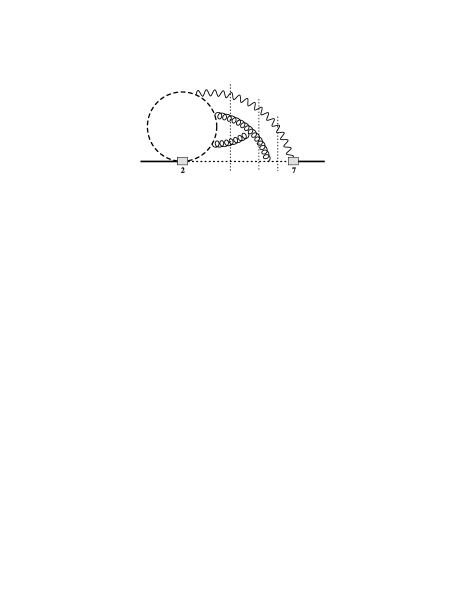
Figure 1: Sample Feynman diagrams contributing to $\hat{G}^{(2)}_{27}$ at ${\mathcal{O}}(\alpha_{\mathrm{s}}^{2})$. The vertical dotted lines indicate possible unitarity cuts. The dotted, dashed and solid propagators correspond to quarks with masses $0$, $m_{c}$ and $m_{b}$, respectively.

Perturbative calculations of $P(E_{0})$ are most conveniently performed in the framework of an effective theory obtained from the SM via decoupling of the $W$ boson and all the heavier particles. The relevant weak interactions are then given by the following Lagrangian density

$${\mathcal{L}}_{\rm weak}=\frac{4G_{F}}{\sqrt{2}}V_{ts}^{\star}V_{tb}\sum_{i=1}^{8}C_{i}(\mu_{b})Q_{i}.$$ (4)

Evaluation of the Wilson coefficients $C_{i}$ to the NNLO accuracy $\left({\mathcal{O}}(\alpha_{\mathrm{s}}^{2})\right)$ at the renormalization scale $\mu_{b}\sim m_{b}$ required computing electroweak-scale matching up to three loops Misiak:2004ew , and QCD anomalous dimensions up to four loops Czakon:2006ss . Since $C_{i}$ in the SM have no imaginary parts, one can write the perturbative decay rate as

$$\Gamma(b\rightarrow X^{p}_{s}\gamma)=\frac{G_{F}^{2}\,m^{5}_{b,\,{\rm pole}}\,\alpha_{\mathrm{e}m}}{32\pi^{4}}\left|V_{ts}^{*}V_{tb}\right|^{2}\sum_{i,j=1}^{8}C_{i}(\mu_{b})C_{j}(\mu_{b})\hat{G}_{ij},\hskip 42.67912pt(\hat{G}_{ij}=\hat{G}_{ji}),$$ (5)

where $\hat{G}_{ij}$ come from interferences of amplitudes with insertions of the operators $Q_{i}$ and $Q_{j}$. The dominant NNLO effects come from $\hat{G}_{17}$, $\hat{G}_{27}$ and $\hat{G}_{77}$ that originate from the operators

$$Q_{1}=(\bar{s}_{L}\gamma_{\mu}T^{a}c_{L})(\bar{c}_{L}\gamma^{\mu}T^{a}b_{L}),\hskip 22.76219ptQ_{2}=(\bar{s}_{L}\gamma_{\mu}c_{L})(\bar{c}_{L}\gamma^{\mu}b_{L}),\hskip 22.76219ptQ_{7}={\textstyle\frac{em_{b}}{16\pi^{2}}}(\bar{s}_{L}\sigma^{\mu\nu}b_{R})F_{\mu\nu}.$$ (6)

Whereas $\hat{G}_{77}$ has been known up to ${\mathcal{O}}(\alpha_{\mathrm{s}}^{2})$ since a long time Blokland:2005uk ; Melnikov:2005bx ; Asatrian:2006ph ; Asatrian:2006sm ; Asatrian:2006rq , no complete NNLO calculation of $\hat{G}_{17}$ and $\hat{G}_{27}$ at the physical value of the charm quark mass $m_{c}$ has been finalized to date. Instead, calculations of these quantities at $m_{c}\gg m_{b}$ Misiak:2006ab ; Misiak:2010sk and $m_{c}=0$ Czakon:2015exa gave a basis for estimating their physical values using interpolation Czakon:2015exa . The related uncertainty in ${\mathcal{B}}_{s\gamma}$ (due to the $m_{c}$-interpolation only) has been estimated at the level of $\pm 3\%$, which places it among the dominant contributions to the overall theoretical uncertainty (see Sec. 3).

To calculate the interferences $\hat{G}_{ij}$ at the physical value of $m_{c}$, it is convenient to express them in terms of propagator diagrams with unitarity cuts. Examples of such four-loop diagrams contributing to $\hat{G}_{27}$ at ${\mathcal{O}}(\alpha_{\mathrm{s}}^{2})$ are shown in Fig. 1, with the light quarks ($u$, $d$, $s$) treated as massless. Similar diagrams for $\hat{G}_{17}$ differ from the $\hat{G}_{27}$ ones by simple colour factors only. For definiteness, we shall focus on $\hat{G}_{27}$ in what follows.

Figure 2: Sample three-loop propagator-type integrals that parameterize large-$z$ expansions of the MIs. Massless and massive internal propagators are denoted by dotted and solid lines, respectively. The thin dotted lines indicate the unitarity cuts.

By analogy to what has been done in the $\hat{G}_{77}$ case Blokland:2005uk ; Melnikov:2005bx ; Asatrian:2006ph ; Asatrian:2006sm ; Asatrian:2006rq , evaluation of ${\mathcal{O}}(\alpha_{\mathrm{s}}^{2})$ contributions to $\hat{G}_{27}$ is performed in two steps. First, no restriction on the photon energy $E_{\gamma}$ is assumed. Next, one performs the calculation for $E_{\gamma}<E_{0}$, which requires considering diagrams with three- and four-body cuts only. The desired result $\hat{G}_{27}^{E_{\gamma}>E_{0}}=\hat{G}_{27}^{{\rm any}\,E_{\gamma}}-\hat{G}_{27}^{E_{\gamma}<E_{0}}$ is then obtained without necessity of determining the differential photon spectrum close to the endpoint $E_{\gamma}^{\rm max}=\frac{1}{2}m_{b}$.

In the present paper, we describe our calculation of $\hat{G}_{27}^{(2)}$ in

$$\hat{G}_{27}~{}=~{}\frac{\alpha_{\mathrm{s}}}{4\pi}\,\hat{G}_{27}^{(1)}~{}+~{}\left(\frac{\alpha_{\mathrm{s}}}{4\pi}\right)^{2}\hat{G}_{27}^{(2)}~{}+~{}{\mathcal{O}}(\alpha_{\mathrm{s}}^{3})$$ (7)

at the physical value of $m_{c}$, and with no restriction on $E_{\gamma}$. Final results are presented for contributions originating from diagrams with closed fermion loops on the gluon lines, like those in the first row of Fig. 1. They undergo separate renormalization and are gauge invariant on their own, so they serve as a useful test case for our calculation of the complete $\hat{G}_{27}^{(2)}$. Most of such contributions have already been determined in the past Ligeti:1999ea ; Bieri:2003ue ; Boughezal:2007ny ; Misiak:2010tk and implemented in the phenomenological analysis Misiak:2015xwa ; Czakon:2015exa . We confirm the published results, and supplement them with a previously uncalculated piece. Some of the previous results have been obtained by a single group only, which makes our verification relevant.

The article is organized as follows. In the next section, our algorithm for evaluation of the complete $\hat{G}_{27}^{(2)}$ is sketched, and the current status of the calculation is summarized. Next, we focus on the closed fermionic loop contributions, displaying our numerical results and comparing them with the literature wherever possible. In Sec. 3, the SM prediction for the branching ratio is updated, taking into account the recently improved estimates of non-perturbative effects Gunawardana:2019gep . We conclude in Sec. 4. In the Appendix, large-$z$ expansions of our final results are presented, and one of the counterterm contributions is discussed.

2 The NNLO contribution to $\hat{G}_{27}$

The quantity $\hat{G}_{27}^{(2)}$ is given by a few hundreds of four-loop propagator diagrams with unitarity cuts, as those presented in Fig. 1. We generate them using QGRAF Nogueira:1991ex and/or FeynArts Kublbeck:1990xc ; Hahn:2000kx . After performing the Dirac algebra with the help of FORM Ruijl:2017dtg , we express the full $\hat{G}_{27}^{(2)}$ in terms of several hundred thousands scalar integrals grouped in ${\mathcal{O}}(500)$ families. Next, the Integration By Parts (IBP) identities Tkachov:1981wb ; Chetyrkin:1981qh ; Laporta:2001dd for each family are generated and applied using KIRA Maierhoefer:2017hyi ; Maierhofer:2018gpa , as well as FIRE Smirnov:2014hma ; Smirnov:2019qkx and LiteRed Lee:2012cn ; Lee:2013mka . In effect, $\hat{G}_{27}^{(2)}$ becomes a linear combination of Master Integrals (MIs). The IBP reduction is the most computer-power demanding part of the calculation, with ${\mathcal{O}}(1\,{\rm TB})$ RAM nodes and weeks of CPU time needed for the most complicated families.

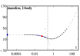
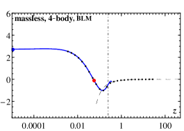
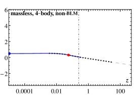
Figure 3: Contributions to $\hat{G}_{27}^{(2)}$ from diagrams with closed loops of massless fermions - see the text. They have already been multiplied by $n_{l}=3$, i.e. the number of flavours we treat as massless.

After setting the renormalization scale squared to $\mu_{b}^{2}=e^{\gamma}m_{b}^{2}/(4\pi)$ (with $\gamma$ being the Euler-Mascheroni constant), the MIs are multiplied by appropriate powers of $m_{b}$, to make them dimensionless. They depend on two parameters only: the dimensional regularization parameter $\epsilon$, and the quark mass ratio $z=m_{c}^{2}/m_{b}^{2}$. In each family separately, the MIs $M_{k}(z,\epsilon)$ satisfy the Differential Equations (DEs)

$$\frac{d}{dz}M_{k}(z,\epsilon)=\sum_{l}R_{kl}(z,\epsilon)M_{l}(z,\epsilon),$$ (8)

where the rational functions $R_{kl}(z,\epsilon)$ on the r.h.s. are determined Kotikov:1990kg ; Remiddi:1997ny ; Gehrmann:1999as from the IBP, too. Similar equations are explicitly displayed in Eq. (3.6) of Ref. Misiak:2017woa where ultraviolet counterterm contributions to $\hat{G}_{27}^{(2)}$ have been determined.

We solve the DEs using the same method as in Refs. Boughezal:2007ny ; Misiak:2017woa ; ARthesis . The MIs are expanded in $\epsilon$ to appropriate powers, with the expansion coefficients being functions of $z$ only. Boundary conditions for these functions at large $z$ are found using asymptotic expansions Smirnov:2002pj . Next, the variable $z$ is treated as complex, and the DEs are numerically solved along half-ellipses in the $z$-plane, to bypass singularities on the real axis.

In practice, the codes q2e and exp Harlander:1997zb ; Seidensticker:1999bb are used to determine the asymptotic expansions at large $z$. Coefficients at subsequent powers of $1/z$ are given in terms of one-, two- and three-loop single-scale integrals, either massive tadpoles or propagator-type ones with unitarity cuts (see Fig. 2). Only at the level of the latter integrals, we perform cross-family identification, which gives us ${\mathcal{O}}(50)$ essentially different and non-vanishing integrals. They are evaluated SSI using various techniques, in particular the Mellin-Barnes one. Once the large-$z$ expansions are found, numerical solutions of the DEs starting from the boundary at $z=20$ are worked out using the code ZVODE zvode upgraded to quadrupole-double precision with the help of the QD qd computation package. Half-ellipses of various sizes are considered to test the numerical stability.

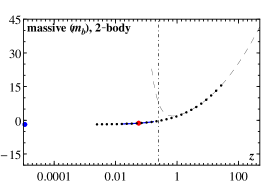
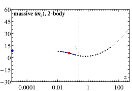
Figure 4: Contributions to $\hat{G}_{27}^{(2)}$ from diagrams with closed loops of massive fermions - see the text.

At present, our IBP reduction for the full $\hat{G}_{27}^{(2)}$ is (almost) completed, and the evaluation of the boundary conditions is being finalized SSI . However, for the diagrams with closed fermionic loops (as the ones in the first row of Fig. 1), the DEs are already solved, and we are ready to present the final results. They are plotted in Figs. 3 and 4 as functions of $z$.

The displayed results correspond to various contributions to $\hat{G}_{27}^{(2)}$ renormalized in the $\overline{\rm MS}$ scheme with $\mu_{b}^{2}=m_{b}^{2}$ (or, equivalently, in the ${\rm MS}$ scheme with $\mu_{b}^{2}=e^{\gamma}m_{b}^{2}/(4\pi)$). The renormalization has been performed with the help of the counterterm contributions evaluated in Refs. Misiak:2017woa ; ARthesis . In all the plots, the black dots correspond to numerical solutions that we have obtained using the DEs. Dots corresponding to the physical value of $z$ are bigger and highlighted in red. Blue dots of similar size on the left boundaries of each plot indicate the $z\to 0$ limits for each contribution, known from the calculation in Ref. Czakon:2015exa . Thin dashed curves continuing to large values of $z$ describe our large-$z$ expansions evaluated up to ${\mathcal{O}}(1/z^{2})$ (see the Appendix). The dash-dotted vertical lines indicate the $c\bar{c}$ production threshold at $z=1/4$, in the vicinity of which neither the large-$z$ nor the small-$z$ expansions are expected to converge well.

In Fig. 3, three distinct contributions from diagrams with closed massless fermion loops are presented. The first (upper left) plot corresponds to diagrams with two-body cuts. The thin dashed line in the small-$z$ region shows the analytic expansion in powers of $z$ evaluated in Ref. Bieri:2003ue . It is the only case for which such an expansion is known. The solid blue curve shows the numerical fit corresponding to Eq. (3.2) of Ref. Boughezal:2007ny where a numerical method (identical to ours) has been used.

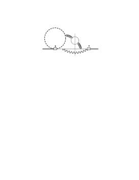
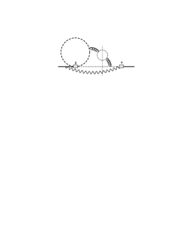
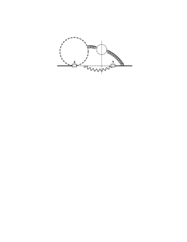
Figure 5: Diagrams corresponding to the last (lower) plot in Fig. 3.

The second (upper right) plot of Fig. 3 shows all the four-body-cut contributions except the diagrams displayed in Fig. 5. The latter diagrams have been skipped in evaluating the photon spectrum in the Brodsky-Lepage-Mackenzie (BLM) Brodsky:1982gc approximation by the authors of Refs. Ligeti:1999ea ; Misiak:2010tk . The solid blue curve is based on the numerical fit from Eq. (3.6) of Ref. Czakon:2015exa that corresponds to no restriction on $E_{\gamma}$, and has been obtained as a by-product of the calculation in Ref. Misiak:2010tk .

The third (bottom) plot in Fig. 3 corresponds to the very diagrams from Fig. 5. In this case, no numerical result valid for arbitrary $m_{c}$ has existed prior to our present calculation. For $z<\frac{1}{4}$, we can describe our findings by the following fit:

$$\Delta^{\mbox{\tiny 4-b \cancel{BLM}}}_{\scriptscriptstyle m=0}\hat{G}_{27}^{(2)}=3\left[0.164+0.13\,z^{\frac{1}{2}}-21.51\,z+68.10\,z^{\frac{3}{2}}-46.12\,z^{2}+(-3.23\,z+18.23\,z^{2})\ln z\right].~{}$$ (9)

It is shown as a solid blue curve in the considered plot. A quick look at Fig. 5 is sufficient to realize that $\Delta^{\mbox{\tiny 4-b \cancel{BLM}}}_{\scriptscriptstyle m=0}\hat{G}_{17}^{(2)}=-\frac{1}{6}\Delta^{\mbox{\tiny 4-b \cancel{BLM}}}_{\scriptscriptstyle m=0}\hat{G}_{27}^{(2)}$, due to the identity $T^{a}T^{b}T^{a}=-\frac{1}{6}T^{b}$ for the $SU(3)_{c}$ generators. The same relative colour factor is valid for all the plots in Figs. 3 and 4.

Fig. 4 shows contributions to $\hat{G}_{27}^{(2)}$ from diagrams with closed loops of quarks with masses $m_{b}$ (left) and $m_{c}$ (right). Only the two-body cuts are included. The solid blue lines correspond to the numerical fits from Eqs. (3.3) and (3.4) of Ref. Boughezal:2007ny . In these cases, no four-body cuts are allowed, as the state $X^{p}_{s}$ in Eq. (5) is assumed to contain no charm quarks. We do not consider three-body cuts here, as their effect can be included by multiplying the well-known three-body contribution to $\hat{G}_{27}^{(1)}$ by finite coefficients originating from $\;Z_{G}^{\rm OS}Z_{g}^{2}-1$. The corresponding term in Eq. (3.8) of Ref. Czakon:2015exa comes at the end of the first line of the expression for $K_{27}^{(2)}$.

As evident from the plots, our results are in perfect agreement with all the previously available expansions and fits. It is particularly important in the massive case (Fig. 4) where our verification comes as the first one from an independent group. Let us note that the contribution displayed in the right plot of Fig. 4 affects ${\mathcal{B}}_{s\gamma}$ by around $-2.1\%$, which should be compared to the current ($\pm 4.5\%$) and expected future ($\pm 2.6\%$) experimental accuracies mentioned in Sec. 1. The massless results from the upper two plots of Fig. 3 have already been cross-checked before.

As far as the new contribution (the third plot in Fig. 3) is concerned, it has so far been included in the interpolated part of the NNLO correction, and resulted in a tiny effect, around one per-mille of the decay rate only. Now we remove it from the interpolated part and replace by the fit in Eq. (9). It turns out that the interpolation estimate was correct within  $\sim\!\!10\%$ of the considered contribution, so the effect remains tiny.

3 Updated SM predictions for ${\mathcal{B}}_{s\gamma}$ and $R_{\gamma}$

In the present section, we work out updated SM predictions for ${\mathcal{B}}_{s\gamma}$, as well as for the ratio $R_{\gamma}\equiv{\mathcal{B}}_{(s+d)\gamma}/{\mathcal{B}}_{c\ell\bar{\nu}}$, where ${\mathcal{B}}_{c\ell\bar{\nu}}$ is the CP- and isospin-averaged branching ratio of the inclusive semileptonic decay. Our main motivation for performing an update right now is not due to the NNLO corrections evaluated in the previous section. The new contribution is tiny, while the sizeable ones (that we have confirmed) were already included in the phenomenological analysis of Ref. Czakon:2015exa . However, there has been an important progress in estimating non-perturbative effects (see below). An update of the SM prediction should thus be performed right now, even though the $m_{c}$-interpolation uncertainty remains essentially unchanged.

The first improvement in estimating the non-perturbative effects becomes possible thanks to the new Belle measurement of the isospin asymmetry

$$\Delta_{0-}\equiv\frac{\Gamma[\bar{B}^{0}\to X_{s}\gamma]-\Gamma[B^{-}\to X_{s}\gamma]}{\Gamma[\bar{B}^{0}\to X_{s}\gamma]+\Gamma[B^{-}\to X_{s}\gamma]}=(-0.48\pm 1.49\pm 0.97\pm 1.15)\%~{}\mbox{\cite[cite]{\@@bibref{Authors Phrase1YearPhrase2}{Watanuki:2018xxg}{\@@citephrase{(}}{\@@citephrase{)}}}}.$$ (10)

In the SM, the dominant contribution to this asymmetry arises from a process where no hard photon but rather a hard gluon is emitted in the $b$-quark decay Lee:2006wn . Next, the gluon scatters on the valence quark, which results in emission of a hard photon. Instead of the valence quark, also a sea quark ($u$, $d$ or $s$) can participate in such a Compton-like scattering. Taking this fact into account, one can write the decay rates as

$$\Gamma[B^{-\!}\to X_{s}\gamma] \simeq A+BQ_{u}+CQ_{d}+DQ_{s},$$

$$\Gamma[\bar{B}^{0\,}\to X_{s}\gamma] \simeq A+BQ_{d}+CQ_{u}+DQ_{s},$$ (11)

where $Q_{u,d,s}$ denote electric charges of the quarks participating in the Compton-like scattering, while the quantities $A$, …, $D$ are given by interferences of various quantum amplitudes whose explicit form is inessential here. Since the considered effect gives only a small correction to the decay rate ($B,C,D\ll A$), quadratic terms in $Q_{u,d,s}$ have been neglected above. We have also neglected isospin violation in the quark masses ($m_{u}\neq m_{d}$) and in the electromagnetic corrections to the $\bar{B}$-meson wave functions (suppressed by extra powers of $\alpha_{em}$).

The leading term $A$ contains the dominant contribution originating from the operator $Q_{7}$. The corrections $B$, $C$, $D$ are suppressed w.r.t. $A$ both by $g_{s}^{2}$ (as the gluon is hard) and by $\Lambda/m_{b}$, with $\Lambda\sim\Lambda_{\rm QCD}$. The latter suppression can be intuitively understood by realizing that the gluon scatters on remnants of the $\bar{B}$ meson, i.e. on a diluted target whose size scales like $1/\Lambda$. Such a suppression is confirmed in Refs. Lee:2006wn ; Benzke:2010js where the Soft-Collinear Effective Theory (SCET) has been applied to analyze non-perturbative corrections to ${\mathcal{B}}_{s\gamma}$.

From Eq. (11), one easily obtains the isospin-averaged decay rate

$$\Gamma\simeq A+\frac{1}{2}(B+C)(Q_{u}+Q_{d})+DQ_{s}\equiv A+\delta\Gamma_{c},$$ (12)

and the isospin asymmetry

$$\Delta_{0-}\simeq\frac{C-B}{2\Gamma}(Q_{u}-Q_{d}).$$ (13)

It follows that the relative correction to the isospin-averaged decay rate that arises due to the considered effect reads

$$\frac{\delta\Gamma_{c}}{\Gamma}\simeq\frac{(B+C)(Q_{u}+Q_{d})+2DQ_{s}}{(C-B)(Q_{u}-Q_{d})}\Delta_{0-}=\frac{Q_{u}+Q_{d}}{Q_{d}-Q_{u}}\left[1+2\,\frac{D-C}{C-B}\right]\Delta_{0-},$$ (14)

where, in the last step, $Q_{s}=-Q_{u}-Q_{d}$ has been used. The second term in the square bracket vanishes in the $SU(3)_{F}$ limit, i.e. when the three lightest quarks are treated as mass-degenerate. In this limit, as observed in Ref. Misiak:2009nr ,  $\delta\Gamma_{c}/\Gamma$  and  $\Delta_{0-}$  are related to each other in a simple manner that is free from non-perturbative uncertainties. The authors of Ref. Benzke:2010js suggested $\pm 30\%$ as an uncertainty estimate stemming from the $SU(3)_{F}$-violating effect in Eq. (14). Following this suggestion, we find

$$\frac{\delta\Gamma_{c}}{\Gamma}=-\frac{1}{3}(1\pm 0.3)\Delta_{0-}=(0.16\pm 0.74)\%,$$ (15)

where the experimental errors from Eq. (10) were combined in quadrature, giving $\Delta_{0-}=(-0.48\pm 2.12)\%$; next, the multiplicative factor was taken into account as follows Goodman:1960var :

$$(1\pm 0.3)(-0.48\pm 2.12)\%=\left(-0.48\pm\sqrt{2.12^{2}+(0.3\cdot 0.48)^{2}+(0.3\cdot 2.12)^{2}}\right)\%.$$ (16)

In the above considerations, we have treated the measured $\Delta_{0-}$ in Eq. (10) as already extrapolated from the experimental cutoff of $E_{0}=1.9\,$GeV down to our default $E_{0}=1.6\,$GeV, even though no such extrapolation has actually been done in Ref. Watanuki:2018xxg , i.e. Eq. (10) corresponds to $E_{0}=1.9\,$GeV. A devoted analysis would be necessary to estimate the extrapolation effects in this case. However, we expect such effects to be negligible w.r.t. the experimental uncertainties in Eq. (10).

If the uncertainty on the r.h.s. of Eq. (15) is treated as $1\sigma$ of a Gaussian distribution, then the 95% C.L. range is $[-1.3,+1.6]\%$. The corresponding range $[-1.4,+2.0]\%$ in Sec. 3.5 of Ref. Gunawardana:2019gep is somewhat wider due to a different method of combining uncertainties and using the PDG Tanabashi:2018oca ; PDGupdate central value of  $-0.6\%$  for $\Delta_{0-}$. When determining our SM predictions below, we calculate ${\mathcal{B}}_{s\gamma}$ without including the photon emission from the valence/sea quarks and, in the final step, we multiply by $\left(1+\frac{\delta\Gamma_{c}}{\Gamma}\right)$, employing the number from the r.h.s. of Eq. (15).

Another important non-perturbative correction to be considered arises in the interference of $Q_{1,2}$ and $Q_{7}$. Its presence in the inclusive $\bar{B}\to X_{s}\gamma$ rate was first pointed out in Ref. Voloshin:1996gw . It amounts to around $+3\%$ of ${\mathcal{B}}_{s\gamma}$, as established in Ref. Buchalla:1997ky at the leading order of an expansion in powers of  $m_{b}\Lambda/m_{c}^{2}$.  The corresponding leading contribution to $N(E_{0})$ in Eq. (1) reads

$$\delta N_{V}=-\frac{\mu_{G}^{2}}{27m_{c}^{2}}C_{7}(\mu_{b})\left(C_{2}(\mu_{b})-\frac{1}{6}C_{1}(\mu_{b})\right),$$ (17)

where $\mu_{G}^{2}\simeq 0.3\,{\rm GeV}^{2}$ is one of the HQET parameters that matter in the determination of $C$ in Eq. (2). Since  $m_{b}\Lambda/m_{c}^{2}$  is not a small parameter, the authors of Ref. Benzke:2010js argued that no expansion in its powers can be used at all. Instead, they estimated the considered correction in the framework of SCET, where essential constraints on models of the relevant soft function came from moments of the semileptonic $\bar{B}\to X_{c}\ell\bar{\nu}$ decay spectra. A recent update of these estimates in Ref. Gunawardana:2019gep implies that $\delta N_{V}$ (17) needs to be multiplied by

$$\kappa_{V}=1-\frac{27m_{c}^{2}\Lambda_{17}}{m_{b}\mu_{G}^{2}}=1.2\pm 0.3.$$ (18)

The final numerical value above has been derived by us from ranges for $\Lambda_{17}$ given in Ref. Gunawardana:2019gep , assuming that these ranges can be interpreted as $1\sigma$ ones. The remaining parameters on which $\kappa_{V}$ depends were set to the values corresponding to the widest range for $\Lambda_{17}$ in Ref. Gunawardana:2019gep .

Since the expression for $\delta N_{V}$ (17) is calculated at the leading order in QCD only, the renormalization scheme for $m_{c}^{2}$ in the denominator is unspecified. We assume that the corresponding uncertainty is included in the overall  $\pm 3\%$  higher-order one that is being retained the same as in Ref. Czakon:2015exa . As the total effect from $\delta N_{V}$ amounts to around $3\%$ in ${\mathcal{B}}_{s\gamma}$, uncertainties due to scheme-dependence of $m_{c}$ in $\delta N_{V}$ can safely be treated this way. In our numerical calculations, the quark masses and HQET parameters are included with a full correlation matrix (see Appendix D of Ref. Czakon:2015exa ), except for the very $m_{c}$ in $\delta N_{V}$ that is now fixed to $1.17\,$GeV. The parameter $\kappa_{V}$ (18) will be treated as uncorrelated.

Apart from the two effects we have discussed above, the authors of Ref. Benzke:2010js identified a third source of uncertain contributions to $N(E_{0})$ that arise at the order ${\mathcal{O}}(\Lambda/m_{b})$. They come proportional to $|C_{8}(\mu_{b})|^{2}$, where $C_{8}$ is the Wilson coefficient of the gluonic dipole operator

$$Q_{8}={\textstyle\frac{g_{s}m_{b}}{16\pi^{2}}}(\bar{s}_{L}\sigma^{\mu\nu}T^{a}b_{R})G^{a}_{\mu\nu}.$$ (19)

Previous estimates of these corrections in Refs. Kapustin:1995fk ; Ferroglia:2010xe focused on large collinear logarithms $\ln\frac{m_{b}}{m_{s}}$  that are present in the corresponding contributions to $P(E_{0})$. In Ref. Czakon:2015exa , such logarithms were varied in the range $\left[\ln 10,\ln 50\right]\simeq\left[\ln\frac{m_{B}}{m_{K}},\ln\frac{m_{B}}{m_{\pi}}\right]$, which served as a crude estimate of the very uncertain but otherwise small contributions to ${\mathcal{B}}_{s\gamma}$ where light hadron masses are the physical collinear regulators. However, according to Ref. Benzke:2010js , possible non-perturbative effects that come multiplied by $|C_{8}(\mu_{b})|^{2}$ can be unrelated to collinear logarithms, and affect ${\mathcal{B}}_{s\gamma}$ by relative corrections in the range $[-0.3,1.9]\%$ with respect to the $\frac{m_{b}}{m_{s}}=50$ case, for $\mu_{b}=1.5\,$GeV and $E_{0}=1.6\,$GeV. Numerically, we can reproduce this range by performing a replacement

$$\ln\frac{m_{b}}{m_{s}}\to\kappa_{88}\ln 50\hskip 28.45274pt\mbox{with}\hskip 28.45274pt\kappa_{88}=1.7\pm 1.1$$ (20)

in all the perturbative contributions proportional to $|C_{8}(\mu_{b})|^{2}$.

In the following, we shall treat the quantities $\frac{\delta\Gamma_{c}}{\Gamma}$ (15), $\kappa_{V}$ (18) and $\kappa_{88}$ (20) on equal footing with all the other parameters that ${\mathcal{B}}_{s\gamma}$ depends on. Since they account for all the non-perturbative effects estimated in Refs. Gunawardana:2019gep ; Benzke:2010js , we shall no longer include the overall $\pm 5\%$ non-perturbative uncertainty that entered the analysis of Ref. Czakon:2015exa as an input from Ref. Benzke:2010js . This way we determine our updated SM predictions for ${\mathcal{B}}_{s\gamma}$ and $R_{\gamma}$ in the SM, namely

$${\mathcal{B}}_{s\gamma}=(3.40\pm 0.17)\times 10^{-4}\hskip 28.45274pt\mbox{and}\hskip 28.45274ptR_{\gamma}=(3.35\pm 0.16)\times 10^{-3},$$ (21)

for $E_{0}=1.6\,$GeV. The overall uncertainties have been obtained by combining in quadrature the ones stemming from higher-order effects ($\pm 3\%$), interpolation in $m_{c}$ ($\pm 3\%$), as well as the parametric uncertainty where all the non-perturbative ones are now contained. Not only $\frac{\delta\Gamma_{c}}{\Gamma}$, $\kappa_{V}$ and $\kappa_{88}$ but several other inputs parameterize non-perturbative effects, too, namely the collinear regulators (see above), as well as the HQET parameters that enter either directly or via the semileptonic phase-space factor $C$ (2). In the ${\mathcal{B}}_{s\gamma}$ case, our parametric uncertainty amounts to $\pm 2.5\%$ at present. All the input parameters listed in Appendix D of Ref. Czakon:2015exa have been retained unchanged.

The overall uncertainty in $R_{\gamma}$ (21) amounts to $\pm 4.8\%$, noticeably improved w.r.t. to $\pm 6.7\%$ in Ref. Misiak:2015xwa . The main reason for the improvement comes from the updated estimate in Ref. Gunawardana:2019gep of the non-perturbative uncertainty that stems from $\Lambda_{17}$ in Eq. (18). Further improvement requires removing the $m_{c}$-interpolation, and re-considering the higher-order and parametric uncertainties. If they remain unchanged, the expected future accuracy in the SM prediction for ${\mathcal{B}}_{s\gamma}$ amounts to $\sqrt{3^{2}+2.5^{2}}\,\%\simeq 3.9\%$, still somewhat behind the experimental expectation of $\pm 2.6\%$ that was mentioned above Eq. (1).

In many BSM theories, extra additive contributions $\Delta C_{7,8}$ to the Wilson coefficients of the operators $Q_{7}$ (6) and $Q_{8}$ (19) at the electroweak matching scale $\mu_{0}$ are the only relevant reason for shifting ${\mathcal{B}}_{s\gamma}$ and $R_{\gamma}$ away from the SM predictions. So long as no accidental cancellations occur, effects due to $\Delta C_{7,8}$ must be small whenever the current experimental constraints are satisfied. At such points in the BSM parameter spaces, ${\mathcal{B}}_{s\gamma}$ and $R_{\gamma}$ can accurately be calculated from the following simple linearized expressions

$${\mathcal{B}}_{s\gamma}\times 10^{4} = (3.40\pm 0.17)-8.25\,\Delta C_{7}-2.10\,\Delta C_{8}\,,$$

$$R_{\gamma}\times 10^{3} = (3.35\pm 0.16)-8.08\,\Delta C_{7}-2.06\,\Delta C_{8}\,,$$ (22)

where $\mu_{0}=160\,$GeV has been chosen. The above equations are updates of similar ones in Eq. (10) of Ref. Misiak:2015xwa . Analytic formulae for the Wilson coefficients at $\mu_{0}$ in a wide class of BSM theories can be found in Ref. Bobeth:1999ww .

In the specific case of the Two-Higgs-Doublet Model, Eq. (22) can be replaced by expressions including all the NLO and NNLO QCD matching corrections Hermann:2012fc . The resulting $95\%\,$C.L. lower bound from $R_{\gamma}$ on the charged Higgs boson mass in Model-II, evaluated along the same lines as in Ref. Misiak:2017bgg , yields $800\,$GeV.

4 Summary

We reported on our calculation of the NNLO QCD corrections to ${\mathcal{B}}_{s\gamma}$ without interpolation in $m_{c}$, and presented final results for contributions originating from propagator diagrams with closed fermion loops on the gluon lines. They correspond either to the two-body ($s\gamma$) or four-body ($sq\bar{q}\gamma$) final states. In all the previously investigated cases, we confirmed the results from the literature, some of which had been obtained by a single group only. The new part comes from four diagrams with four-particle cuts that had not been determined before, as they are not included in the BLM approximation. Their contribution turns out to be tiny ($\sim 0.1\%$ of the decay rate) and quite well reproduced by our former interpolation algorithm.

In view of the recent progress in estimating the non-perturbative contributions, we performed an update of the phenomenological analysis within the SM. The obtained results yield  ${\mathcal{B}}_{s\gamma}=(3.40\pm 0.17)\times 10^{-4}$  and  $R_{\gamma}\equiv{\mathcal{B}}_{(s+d)\gamma}/{\mathcal{B}}_{c\ell\bar{\nu}}=(3.35\pm 0.16)\times 10^{-3}$  for  $E_{0}=1.6\,$GeV. The main improvement in the uncertainty came from the analysis in Ref. Gunawardana:2019gep where non-perturbative effects in the $Q_{1,2}$-$Q_{7}$ interference were re-analyzed.

The next contribution to suppressing the overall theoretical uncertainty is expected from the calculation of $\hat{G}_{17}^{(2)}$ and $\hat{G}_{27}^{(2)}$ for $E_{0}=0$ and at the physical value of $m_{c}$, thereby removing the need for $m_{c}$-interpolation in these quantities.

Note added in the proofs

While the present article was being reviewed for publication, a new paper Benzke:2020htm on non-perturbative effects in the $Q_{1,2}$-$Q_{7}$ interference appeared on the arXiv. To replace the estimates of Ref. Gunawardana:2019gep by those of Ref. Benzke:2020htm in our approach, one would need to use $\kappa_{V}=1.7\pm 0.8$ in Eq. (18). This would shift our prediction for ${\mathcal{B}}_{s\gamma}$ from $(3.40\pm 0.17)\times 10^{-4}$ to $(3.45\pm 0.19)\times 10^{-4}$, and strengthen the constraint on $M_{H^{\pm}}$ even more. However, the extreme values of $\Lambda_{17}$ in Ref. Benzke:2020htm originate from soft function models with quite a rich structure. Such soft functions are related to energy-momentum distributions of gluons inside the QCD ground states ($B$ mesons), in which case encountering large numbers of extrema and zero points seems unlikely. Therefore, our preference is to retain $\kappa_{V}$ as it stands in Eq. (18) for evaluating the SM predictions for ${\mathcal{B}}_{s\gamma}$ and $R_{\gamma}$.

Appendix: Large-$z$ expansions and $\hat{G}_{47}^{(1)}$ with charm loops

In this appendix, we present large-$z$ expansions of the renormalized contributions to $\hat{G}_{27}^{(2)}$ plotted in Figs. 3 and 4. They are shown by the thin dashed lines reaching large values of $z$ in the corresponding plots. For the three plots in Fig. 3 that describe contributions from diagrams with closed loops of massless fermions, the respective expansions read

$$\Delta^{\mbox{\tiny 2-b}}_{\scriptscriptstyle m=0}\hat{G}_{27}^{(2)} = 3\left[{\textstyle\frac{27650}{6561}}+{\textstyle\frac{112}{243}}L+{\textstyle\frac{8}{9}}L^{2}+{\textstyle\frac{1}{z}}\left({\textstyle\frac{10427}{30375}}-{\textstyle\frac{8}{135}}\pi^{2}-{\textstyle\frac{572}{18225}}L+{\textstyle\frac{38}{405}}L^{2}\right)\right.$$

$$+ \left.{\textstyle\frac{1}{z^{2}}}\left({\textstyle\frac{19899293}{125023500}}-{\textstyle\frac{8}{405}}\pi^{2}-{\textstyle\frac{1628}{893025}}L+{\textstyle\frac{86}{2835}}L^{2}\right)\right]+{\mathcal{O}}\left({\textstyle\frac{1}{z^{3}}}\right),$$

$$\Delta^{\mbox{\tiny 4-b BLM}}_{\scriptscriptstyle m=0}\,\hat{G}_{27}^{(2)} = 3\left[{\textstyle\frac{1}{z}}\left({\textstyle\frac{41}{108}}-{\textstyle\frac{10}{243}}\pi^{2}\right)+{\textstyle\frac{1}{z^{2}}}\left({\textstyle\frac{487}{3375}}-{\textstyle\frac{2}{135}}\pi^{2}\right)\right]+{\mathcal{O}}\left({\textstyle\frac{1}{z^{3}}}\right),$$

$$\Delta^{\mbox{\tiny 4-b \cancel{BLM}}}_{\scriptscriptstyle m=0}\,\hat{G}_{27}^{(2)} = 3\left[-{\textstyle\frac{32}{729}}(1+L)+{\textstyle\frac{1}{z}}\left(-{\textstyle\frac{941}{7290}}+{\textstyle\frac{16}{1215}}\pi^{2}\right)+{\textstyle\frac{1}{z^{2}}}\left(-{\textstyle\frac{10852}{212625}}+{\textstyle\frac{44}{8505}}\pi^{2}\right)\right]+{\mathcal{O}}\left({\textstyle\frac{1}{z^{3}}}\right),$$

(A.23)

where $L=\ln z$. The first expression above coincides with Eq. (5.3) of Ref. Misiak:2006ab .

For the closed bottom loops (the left plot in Fig. 4), we find

$$\Delta^{\mbox{\tiny 2-b}}_{\scriptscriptstyle m=m_{b}}\hat{G}_{27}^{(2)} = {\textstyle\frac{62210}{6561}}+{\textstyle\frac{160}{729}}\pi^{2}-{\textstyle\frac{16\pi}{9\sqrt{3}}}-16S_{2}+\left({\textstyle\frac{464}{81}}+{\textstyle\frac{160}{729}}\pi^{2}-{\textstyle\frac{16\pi}{9\sqrt{3}}}-16S_{2}\right)L+{\textstyle\frac{8}{9}}L^{2}$$ (A.24)

$$+ {\textstyle\frac{1}{z}}\left(-{\textstyle\frac{30991}{10125}}+{\textstyle\frac{656}{3645}}\pi^{2}+{\textstyle\frac{4\pi}{45\sqrt{3}}}+{\textstyle\frac{64}{405}}\zeta_{3}+{\textstyle\frac{4}{5}}S_{2}-{\textstyle\frac{32972}{18225}}L+{\textstyle\frac{38}{405}}L^{2}\right)$$

$$+~{}~{}{\textstyle\frac{1}{z^{2}}}\left(-{\textstyle\frac{38874763}{25004700}}-{\textstyle\frac{8}{1701}}\pi^{2}+{\textstyle\frac{26\pi}{525\sqrt{3}}}+{\textstyle\frac{64}{2835}}\zeta_{3}+{\textstyle\frac{12}{35}}S_{2}-{\textstyle\frac{864896}{893025}}L-{\textstyle\frac{418}{2835}}L^{2}\right)+{\mathcal{O}}\left({\textstyle\frac{1}{z^{3}}}\right),$$

where $S_{2}=\frac{4}{9\sqrt{3}}\,{\rm Im}\!\left[{\rm Li}_{2}\left(e^{i\pi/3}\right)\right]$. Finally, for the closed charm loops (the right plot in Fig. 4), the large-$z$ expansion reads

$$\Delta^{\mbox{\tiny 2-b}}_{\scriptscriptstyle m=m_{c}}\hat{G}_{27}^{(2)} = {\textstyle\frac{11018}{6561}}+{\textstyle\frac{128}{243}}L+{\textstyle\frac{200}{243}}L^{2}+{\textstyle\frac{1}{z}}\left({\textstyle\frac{5714}{54675}}+{\textstyle\frac{7}{81}}\zeta_{3}+{\textstyle\frac{2146}{18225}}L+{\textstyle\frac{52}{405}}L^{2}\right)$$ (A.25)

$$+ {\textstyle\frac{1}{z^{2}}}\left(-{\textstyle\frac{62075113}{428652000}}+{\textstyle\frac{469}{5184}}\zeta_{3}-{\textstyle\frac{41987}{893025}}L+{\textstyle\frac{92}{2835}}L^{2}\right)+{\mathcal{O}}\left({\textstyle\frac{1}{z^{3}}}\right).$$

Our results in Eqs. (A.24) and (A.25) agree with the numerical ones in Eqs. (A.1) and (A.2) of Ref. Boughezal:2007ny . Analytical expressions for the leading terms agree with the findings of Ref. Misiak:2010sk .

Determining the renormalized results plotted in Figs. 3 and 4 required taking into account $\hat{G}_{47}^{(1){\rm bare}}$, i.e. three-loop counterterm diagrams with vertices proportional to $Q_{4}=(\bar{s}_{L}\gamma_{\mu}T^{a}b_{L})\sum_{q}(\bar{q}\gamma^{\mu}T^{a}q)$. An expression for this quantity in Eq. (2.4) of Ref. Czakon:2015exa contains no contributions from closed loops of charm quarks, as all the other results in Sec. 2 of that paper. Such contributions arise in the two-body channel only. They take the form

$$\Delta^{\mbox{\tiny 2-b}}_{\scriptscriptstyle m=m_{c}}\hat{G}_{47}^{(1){\rm bare}}={\textstyle\frac{16}{81\epsilon}}-{\textstyle\frac{4}{243}}+{\textstyle\frac{264\pi^{2}-2186}{729}}\epsilon+2{\rm Re}\left[b(z)+\epsilon\tilde{b}(z)\right]+{\mathcal{O}}(\epsilon^{2}).$$ (A.26)

Small-$z$ expansion of the function $b(z)$ has been given in Eq. (3.9) of Ref. Buras:2002tp , while the large-$z$ expansion of ${\rm Re}\,b(z)$ can be found Eq. (5.2) of Ref. Misiak:2006ab . As far as $\tilde{b}(z)$ is concerned, we obtain the following expansions:

$${\rm Re}\,\tilde{b}(z) = {\textstyle\frac{1144}{729}}-{\textstyle\frac{46}{243}}\pi^{2}-{\textstyle\frac{8}{243}}L-{\textstyle\frac{2}{81}}L^{2}+{\textstyle\frac{1}{z}}\left({\textstyle\frac{10957}{60750}}+{\textstyle\frac{212}{2025}}L+{\textstyle\frac{1}{15}}L^{2}\right)$$

$$+ {\textstyle\frac{1}{z^{2}}}\left({\textstyle\frac{491839}{41674500}}+{\textstyle\frac{134}{33075}}L+{\textstyle\frac{2}{63}}L^{2}\right)+{\mathcal{O}}\left({\textstyle\frac{1}{z^{3}}}\right),$$

$${\rm Re}\,\tilde{b}(z) = \left({\textstyle\frac{44}{3}}-{\textstyle\frac{16}{9}}\pi^{2}-{\textstyle\frac{40}{9}}\zeta_{3}+{\textstyle\frac{16}{9}}L-{\textstyle\frac{8}{9}}L^{2}\right)z+\left({\textstyle\frac{304}{81}}-{\textstyle\frac{128}{27}}\ln 2-{\textstyle\frac{32}{27}}L\right)\pi^{2}z^{\frac{3}{2}}$$ (A.27)

$$+ \left({\textstyle\frac{53}{3}}-{\textstyle\frac{20}{27}}\pi^{2}+{\textstyle\frac{14}{3}}L-{\textstyle\frac{32}{27}}\pi^{2}L+{\textstyle\frac{10}{9}}L^{2}-{\textstyle\frac{4}{9}}L^{3}\right)z^{2}-{\textstyle\frac{80}{27}}\pi^{2}z^{\frac{5}{2}}$$

$$+ \left({\textstyle\frac{6830}{729}}-{\textstyle\frac{292}{243}}\pi^{2}+{\textstyle\frac{80}{27}}\zeta_{3}+{\textstyle\frac{68}{243}}L+{\textstyle\frac{64}{81}}\pi^{2}L-{\textstyle\frac{124}{27}}L^{2}+{\textstyle\frac{16}{9}}L^{3}\right)z^{3}+{\textstyle\frac{88}{135}}\pi^{2}z^{\frac{7}{2}}$$

$$+ \left({\textstyle\frac{1944727}{121500}}-{\textstyle\frac{304}{405}}\pi^{2}+{\textstyle\frac{32}{9}}\zeta_{3}-{\textstyle\frac{17239}{2025}}L-{\textstyle\frac{80}{27}}L^{2}+{\textstyle\frac{16}{9}}L^{3}\right)z^{4}+{\textstyle\frac{272}{2835}}\pi^{2}z^{\frac{9}{2}}$$

$$+ \left({\textstyle\frac{34017647}{833490}}-{\textstyle\frac{1018}{189}}\pi^{2}+{\textstyle\frac{80}{9}}\zeta_{3}-{\textstyle\frac{113308}{3969}}L-{\textstyle\frac{182}{27}}L^{2}+{\textstyle\frac{40}{9}}L^{3}\right)z^{5}+{\mathcal{O}}\left(z^{\frac{11}{2}}\right).$$

No explicit expressions for the expansions of $\tilde{b}(z)$ have so far been published, even though this function must have been used for UV renormalization in Ref. Boughezal:2007ny .

References

- (1) S. L. Glashow, J. Iliopoulos and L. Maiani, Phys. Rev. D 2 (1970) 1285.
- (2) J. Aebischer, W. Altmannshofer, D. Guadagnoli, M. Reboud, P. Stangl and D. M. Straub, Eur. Phys. J. C 80 (2020) 252 [arXiv:1903.10434].
- (3) S. Chen et al. (CLEO Collaboration), Phys. Rev. Lett. 87 (2001) 251807 [hep-ex/0108032].
- (4) B. Aubert et al. (BaBar Collaboration), Phys. Rev. D 77 (2008) 051103 [arXiv:0711.4889].
- (5) J. P. Lees et al. (BaBar Collaboration), Phys. Rev. D 86 (2012) 052012 [arXiv:1207.2520].
- (6) J. P. Lees et al. (BaBar Collaboration), Phys. Rev. Lett. 109 (2012) 191801 [arXiv:1207.2690].
- (7) T. Saito et al. (Belle Collaboration), Phys. Rev. D 91 (2015) 052004 [arXiv:1411.7198].
- (8) A. Abdesselam et al. (Belle Collaboration), arXiv:1608.02344.
- (9) Y. S. Amhis et al. (HFLAV Collaboration), arXiv:1909.12524.
- (10) E. Kou et al. (Belle-II Collaboration), PTEP 2019 (2019) 123C01 [arXiv:1808.10567].
- (11) A. Ishikawa, talk at the “7th Workshop on Rare Semileptonic Decays”, September 4-6th, 2019, Lyon, France, https://indico.in2p3.fr/event/18646 .
- (12) M. Misiak, H. Asatrian, R. Boughezal, M. Czakon, T. Ewerth, A. Ferroglia, P. Fiedler, P. Gambino, C. Greub, U. Haisch, T. Huber, M. Kamiński, G. Ossola, M. Poradziński, A. Rehman, T. Schutzmeier, M. Steinhauser and J. Virto, Phys. Rev. Lett. 114 (2015) 221801 [arXiv:1503.01789].
- (13) M. Czakon, P. Fiedler, T. Huber, M. Misiak, T. Schutzmeier and M. Steinhauser, JHEP 1504 (2015) 168 [arXiv:1503.01791].
- (14) A. Alberti, P. Gambino, K. J. Healey and S. Nandi, Phys. Rev. Lett. 114 (2015) 061802 [arXiv:1411.6560].
- (15) M. Misiak and M. Steinhauser, Nucl. Phys. B 683 (2004) 277 [hep-ph/0401041].
- (16) M. Czakon, U. Haisch and M. Misiak, JHEP 0703 (2007) 008 [hep-ph/0612329].
- (17) I. R. Blokland, A. Czarnecki, M. Misiak, M. Ślusarczyk and F. Tkachov, Phys. Rev. D 72 (2005) 033014 [hep-ph/0506055].
- (18) K. Melnikov and A. Mitov, Phys. Lett. B 620 (2005) 69 [hep-ph/0505097].
- (19) H. M. Asatrian, A. Hovhannisyan, V. Poghosyan, T. Ewerth, C. Greub and T. Hurth, Nucl. Phys. B 749 (2006) 325 [hep-ph/0605009].
- (20) H. M. Asatrian, T. Ewerth, A. Ferroglia, P. Gambino and C. Greub, Nucl. Phys. B 762 (2007) 212 [hep-ph/0607316].
- (21) H. M. Asatrian, T. Ewerth, H. Gabrielyan and C. Greub, Phys. Lett. B 647 (2007) 173 [hep-ph/0611123].
- (22) M. Misiak and M. Steinhauser, Nucl. Phys. B 764 (2007) 62 [hep-ph/0609241].
- (23) M. Misiak and M. Steinhauser, Nucl. Phys. B 840 (2010) 271 [arXiv:1005.1173].
- (24) Z. Ligeti, M. E. Luke, A. V. Manohar and M. B. Wise, Phys. Rev. D 60 (1999) 034019 [hep-ph/9903305].
- (25) K. Bieri, C. Greub and M. Steinhauser, Phys. Rev. D 67 (2003) 114019 [hep-ph/0302051].
- (26) R. Boughezal, M. Czakon and T. Schutzmeier, JHEP 0709 (2007) 072 [arXiv:0707.3090].
- (27) M. Misiak and M. Poradziński, Phys. Rev. D 83 (2011) 014024 [arXiv:1009.5685].
- (28) A. Gunawardana and G. Paz, JHEP 1911 (2019) 141 [arXiv:1908.02812].
- (29) P. Nogueira, J. Comput. Phys. 105 (1993) 279.
- (30) J. Kublbeck, M. Bohm and A. Denner, Comput. Phys. Commun. 60 (1990) 165.
- (31) T. Hahn, Comput. Phys. Commun. 140 (2001) 418 [hep-ph/0012260].
- (32) B. Ruijl, T. Ueda and J. Vermaseren, arXiv:1707.06453.
- (33) F. V. Tkachov, Phys. Lett. 100B (1981) 65.
- (34) K. G. Chetyrkin and F. V. Tkachov, Nucl. Phys. B 192 (1981) 159.
- (35) S. Laporta, Int. J. Mod. Phys. A 15 (2000) 5087 [hep-ph/0102033].
- (36) P. Maierhöfer, J. Usovitsch and P. Uwer, Comput. Phys. Commun. 230 (2018) 99 [arXiv:1705.05610].
- (37) P. Maierhöfer and J. Usovitsch, arXiv:1812.01491.
- (38) A. V. Smirnov, Comput. Phys. Commun. 189 (2015) 182 [arXiv:1408.2372].
- (39) A. V. Smirnov and F. S. Chuharev, arXiv:1901.07808.
- (40) R. N. Lee, arXiv:1212.2685.
- (41) R. N. Lee, J. Phys. Conf. Ser. 523 (2014) 012059 [arXiv:1310.1145].
- (42) A. V. Kotikov, Phys. Lett. B 254 (1991) 158.
- (43) E. Remiddi, Nuovo Cim. A 110 (1997) 1435 [hep-th/9711188].
- (44) T. Gehrmann and E. Remiddi, Nucl. Phys. B 580 (2000) 485 [hep-ph/9912329].
- (45) M. Misiak, A. Rehman and M. Steinhauser, Phys. Lett. B 770 (2017) 431 [arXiv:1702.07674].
-
(46)
A. Rehman, Ph.D. thesis, University of Warsaw, 2015,
http://depotuw.ceon.pl/handle/item/1197 . - (47) V. A. Smirnov, Springer Tracts Mod. Phys. 177 (2002) 1.
- (48) R. Harlander, T. Seidensticker and M. Steinhauser, Phys. Lett. B 426 (1998) 125 [hep-ph/9712228].
- (49) T. Seidensticker, hep-ph/9905298.
- (50) M. Czaja, T. Huber, G. Mishima, M. Misiak, A. Rehman and M. Steinhauser, in preparation.
-
(51)
P. N. Brown, G. D. Byrne and A. C. Hindmarsh, ZVODE,
http://netlib.sandia.gov/ode/zvode.f . -
(52)
Y. Hida, X.S. Li and D.H. Bailey, QD computation package,
http://crd-legacy.lbl.gov/dhbailey/mpdist . - (53) S. J. Brodsky, G. P. Lepage and P. B. Mackenzie, Phys. Rev. D 28 (1983) 228.
- (54) S. Watanuki et al. (Belle Collaboration), Phys. Rev. D 99 (2019) 032012 [arXiv:1807.04236].
- (55) S. J. Lee, M. Neubert and G. Paz, Phys. Rev. D 75 (2007) 114005 [hep-ph/0609224].
- (56) M. Benzke, S. J. Lee, M. Neubert and G. Paz, JHEP 1008 (2010) 099 [arXiv:1003.5012].
- (57) M. Misiak, Acta Phys. Polon. B 40 (2009) 2987 [arXiv:0911.1651].
- (58) L. A. Goodman, Journal of the American Statistical Association 55 (1960) 708.
-
(59)
M. Tanabashi et al. [Particle Data Group],
Phys. Rev. D 98 (2018) 030001.
-
(60)
Particle Data Group, page 66 in
http://pdg.lbl.gov/2019/listings/rpp2019-list-B-plus-minus-B0-admixture.pdf . - (61) M. B. Voloshin, Phys. Lett. B 397 (1997) 275 [hep-ph/9612483].
- (62) G. Buchalla, G. Isidori and S. J. Rey, Nucl. Phys. B 511 (1998) 594 [hep-ph/9705253].
- (63) A. Kapustin, Z. Ligeti and H. D. Politzer, Phys. Lett. B 357 (1995) 653 [hep-ph/9507248].
- (64) A. Ferroglia and U. Haisch, Phys. Rev. D 82 (2010) 094012 [arXiv:1009.2144].
- (65) C. Bobeth, M. Misiak and J. Urban, Nucl. Phys. B 567 (2000) 153 [hep-ph/9904413].
- (66) T. Hermann, M. Misiak and M. Steinhauser, JHEP 1211 (2012) 036 [arXiv:1208.2788].
- (67) M. Misiak and M. Steinhauser, Eur. Phys. J. C 77 (2017) 201 [arXiv:1702.04571].
- (68) M. Benzke and T. Hurth, arXiv:2006.00624.
- (69) A. J. Buras, A. Czarnecki, M. Misiak and J. Urban, Nucl. Phys. B 631 (2002) 219 [hep-ph/0203135].