Optimal deception attack on networked vehicular cyber physical systems

Abstract

Herein, design of false data injection attack on a distributed cyber-physical system is considered. A stochastic process with linear dynamics and Gaussian noise is measured by multiple agent nodes, each equipped with multiple sensors. The agent nodes form a multi-hop network among themselves. Each agent node computes an estimate of the process by using its sensor observation and messages obtained from neighbouring nodes, via Kalman-consensus filtering. An external attacker, capable of arbitrarily manipulating the sensor observations of some or all agent nodes, injects errors into those sensor observations. The goal of the attacker is to steer the estimates at the agent nodes as close as possible to a pre-specified value, while respecting a constraint on the attack detection probability. To this end, a constrained optimization problem is formulated to find the optimal parameter values of a certain class of linear attacks. The parameters of linear attack are learnt on-line via a combination of stochastic approximation and online stochastic gradient descent. Numerical results demonstrate the efficacy of the attack.

Ginwidth=1.0

I Introduction

In recent times, there have been significant interest in designing cyber-physical systems (CPS) that combine the cyber world and the physical world via seamless integration of sensing, computation, communication, control and learning. CPS has widespread applications such as networked monitoring and control of industrial processes, disaster management, smart grids, intelligent transportation systems, etc. These applications critically depend on estimation of a physical process via multiple sensors over a wireless network. However, increasing use of wireless networks in sharing the sensed data has rendered the sensors vulnerable to various cyber-attacks. In this paper, we focus on false data injection (FDI) attacks which is an integrity or deception attack where the attacker modifies the information flowing through the network [1, 2], in contrast to a denial-of-service attack where the attacker blocks system resources (e.g., wireless jamming attack [3]). In FDI, the attacker either breaks the cryptography of the data packets or physically manipulates the sensors (e.g., putting a heater near a temperature sensor).

I-A Related Literature

The cyber-physical systems either need to compute the process estimate in a remote estimator (centralized case), or often multiple nodes or components of the system need to estimate the same process over time via sensor observations and the information shared over a network (distributed case). The problem of FDI attack design and its detection has received significant attention in recent times; attack design: conditions for undetectable FDI attack [4], design of a linear deception attack scheme to fool the popular $\chi^{2}$ detector (see [5]), optimal attack design for noiseless systems [6]. The paper [7] designs an optimal attack to steer the state of a control system to a desired target under a constraint on the attack detection probability. On the other hand, attempts on attack detection includes centralized (and decentralized as well) schemes for noiseless systems [8], coding of sensor output along with $\chi^{2}$ detector [9], comparing the sensor observations with those coming from from a few known safe sensors [10], and the attack detection and secure estimation schemes based on innovation vectors in [11]. Attempts on attack-resilient state estimation include: [12] for bounded noise, [13, 14, 15] for adaptive filter design using stochastic approximation, [16] that uses sparsity models to characterize the switching location attack in a noiseless linear system and state recovery constraints for various attack modes. FDI attack and its mitigation in power systems are addressed in [17, 18, 19]. Attack-resilient state estimation and control in noiseless systems are discussed in [20] and [21]. Performance bound of stealthy attack in a single sensor-remote estimator system using Kalman filter was characterized in [22].

However, there have been very few attempts for attack design and mitigation in distributed CPS, except [23] for attack detection and secure estimation, [24] for attack detection in networked control system using a certain dynamic watermarking strategy, and [25] for attack detection in power systems. To our knowledge, there has been no attempt to theoretically design an attack strategy in distributed CPS.

I-B Our Contribution

In light of the above issues, our contributions in this paper are the following:

1. Under the Kalman-consensus filter (KCF, see [26]) for distributed estimation, we design a novel attack scheme that steers the estimates in all estimators towards a target value, while respecting a constraint on the attack detection probability under the popular $\chi^{2}$ detector adapted to the distributed setting. The attack scheme is reminiscent of the popular linear attack scheme [5], but the novelty lies in online learning of the parameters in the attack algorithm via simultaneous perturbation stochastic approximation (SPSA, see [27]). The attack algorithm, unlike the linear attack scheme of [5], uses a non-zero mean Gaussian perturbation to modify the observation made at a node, and this non-zero mean is an affine function of the process estimate at a node. The optimization problem is cast as an online optimization problem, where SPSA is used for online stochastic gradient descent (see [28, Chapter $3$]).

2. The constraint on attack detection probability is met by updating a Lagrange multiplier via stochastic approximation at a slower timescale.

3. Though the proposed algorithm involves on-line parameter learning, it can be used off-line to optimize the attack parameters which can then be used in real CPS.

I-C Organization

The rest of the paper is organized as follows. System model and the necessary background related to the problem are provided in Section II. The attack design algorithm is developed in Section III, and its performance in evaluated numerically in Section IV. Conclusions are made in Section V.

II System Model and Background

In this paper, bold capital letters, bold small letters and capital letters with caligraphic font will denote matrices, vectors and sets respectively.

II-A Sensing and estimation model

We consider a connected, multihop wireless network (see Figure 1) of $N$ agent nodes denoted by $\mathcal{N}\doteq\{1,2,\cdots,N\}$. The set of neighbouring nodes of node $k$ is denoted by $\mathcal{N}_{k}$, and let $N_{k}\doteq|\mathcal{N}_{k}|$. There is a discrete-time stochastic process $\{\bm{x}(t)\}_{t\geq 0}$ (where $\bm{x}(t)\in\mathbb{R}^{q}$) which is a linear Gaussian process evolving as follows:

$$\bm{x}(t+1)=\bm{A}\bm{x}(t)+\underbrace{\bm{w}(t)}_{\sim\mathcal{N}(\bm{0},\bm{Q})}$$ (1)

where $\bm{w}(t)$ is zero-mean i.i.d. Gaussian noise.

Each agent node is equipped with one or more sensors who make some observation about the process. The vector observation received at node $k$ at time $t$ is given by:

$$\bm{y}_{k}(t)=\bm{H}_{k}\bm{x}(t)+\underbrace{\bm{v}_{k}(t)}_{\sim\mathcal{N}(\bm{0},\bm{R}_{k})},$$ (2)

where $\bm{H}_{k}$ is a matrix of appropriate dimension and $\bm{v}_{k}(t)$ is a Gaussian observation noise which is independent across sensors and i.i.d. across $t$.

At time $t$, each agent node $k\in\mathcal{N}$ declares an estimate $\bm{\hat{x}}^{(k)}(t)$ using Kalman consensus filtering (KCF, see [26]) which involves the following sequence of steps:

1. Node $k$ computes an intermediate estimate $\bar{\bm{x}}^{(k)}(t)=\bm{A}\hat{\bm{x}}^{(k)}(t-1)$.

2. Node $k$ broadcasts $\bar{\bm{x}}^{(k)}(t)$ to all $j\in\mathcal{N}_{k}$.

3. Node $k$ computes its final estimate of the process as:

   $$\hat{\bm{x}}^{(k)}(t) = \bar{\bm{x}}^{(k)}(t)+\bm{G}_{k}(\bm{y}_{k}(t)-\bm{H}_{k}\bar{\bm{x}}^{(k)}(t))$$ (3)

   $$+\bm{C}_{k}\sum_{j\in\mathcal{N}_{k}}(\bar{\bm{x}}^{(j)}(t)-\bar{\bm{x}}^{(k)}(t))$$

Here $\bm{G}_{k}$ and $\bm{C}_{k}$ are the Kalman and consensus gain matrices used by node $k$, respectively.

II-B False data injection (FDI) attack

At time $t$, sensors associated to any subset of nodes $\mathcal{A}_{t}\subset\mathcal{N}$ can be under attack. A node $k\in\mathcal{A}_{t}$ receives an observation:

$$\tilde{\bm{y}}_{k}(t)=\bm{H}_{k}\bm{x}(t)+\bm{e}_{k}(t)+\bm{v}_{k}(t),$$ (4)

where $\bm{e}_{k}(t)$ is the error injected by the attacker. The attacker seeks to insert the error sequence $\{\bm{e}_{k}(t):k\in\mathcal{A}_{t}\}_{t\geq 0}$ in order to introduce error in the estimation. If $\mathcal{A}_{t}=\mathcal{A}$ for all $t$, then the attack is called a static attack, otherwise the attack is called a switching location attack. We will consider only static attack in this paper. We assume that the attacker can observe $\hat{\bm{x}}^{(k)}(t)$ for all $1\leq k\leq N$ once they are computed by the agent nodes.

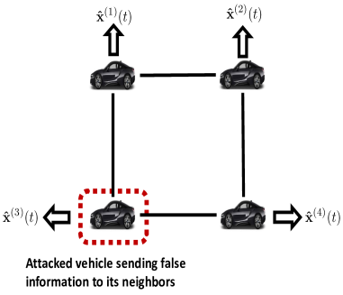
Figure 1: False data injection attack in remote estimation.

II-C The $\chi^{2}$ detector

Let us define the innovation vector at node $k$ by $\bm{z}_{k}(t):=\bm{y}_{k}(t)-\bm{H}_{k}\bm{A}\hat{\bm{x}}^{(k)}(t-1)$. Let us assume that, under no attack, $\{\bm{z}_{k}(t)\}_{t\geq 0}$ reaches its steady-state distribution $N(\bm{0},\bm{\Sigma}_{k})$. Under a possible attack, a standard technique (see [5], [10]) to detect any anomaly in $\{\bm{z}_{t}\}_{t\geq 0}$ is the $\chi^{2}$ detector, which tests whether the innovation vector follows the desired Gaussian distribution. The detector at each agent node observes the innovation sequence over a pre-specified window of $J$ time-slots, and declares an attack at time $\tau$ if $\sum_{t=\tau-J+1}^{\tau}\bm{z}_{k}(t)^{\prime}\bm{\Sigma}_{k}^{-1}\bm{z}_{k}(t)\geq\eta$, where $\eta$ is a threshold which can be adjusted to control the false alarm probability. The covariance matrix $\bm{\Sigma}_{k}$ can be computed from standard results on KCF as in [26].

The authors of [5] proposed a linear injection attack to fool the $\chi^{2}$ detector in a centralized, remote estimation setting. Motivated by [5], we also propose a linear attack, where, at time $t$, the sensor(s) associated with any node $k\in\mathcal{A}$ modifies the innovation vector as $\bm{\tilde{z}_{k}}(t)=\bm{T}_{k}\bm{z}_{k}(t)+\bm{b}_{k}(t)$, where $\bm{T}_{k}$ is a square matrix and $\bm{b}_{k}(t)\sim N(\bm{\mu}_{k}(\bm{\theta}^{(k)}(t-1)),\bm{S}_{k})$ is independent Gaussian. The bias term $\bm{\mu}_{k}(\bm{\theta}^{(k)}(t-1))$ is assumed to take a linear form $\bm{\mu}_{k}(\bm{\theta}^{(k)}(t-1))=\bm{M}_{k}\bm{\theta}^{(k)}(t-1)+\bm{d}_{k}$ for suitable matrices and vectors $\bm{M}_{k}$ and $\bm{d}_{k}$. This is equivalent to modifying the observation vector to $\bm{\tilde{y}_{k}}(t)$. If $\{\bm{T}_{k},\bm{S}_{k},\bm{M}_{k},\bm{d}_{k}\}_{1\leq k\leq N}$ is constant over time $t$, the attack is called stationary, else non-stationary.

II-D The optimization problem

The attacker seeks to steer the estimate as close as possible to some pre-defined value $\bm{x}^{*}$, while keeping the attack detection probability per unit time under some constraint value $\alpha$. Note that, the probability of attack detection per unit time slot can be upper bounded as:

$$P_{d} \leq \limsup_{T\rightarrow\infty}\frac{1}{T+1}\sum_{\tau=0}^{T}\sum_{k=1}^{N}\mathbb{P}(\sum_{t=\tau-J+1}^{\tau}\tilde{\bm{z}}_{k}(t)^{\prime}\bm{\Sigma}_{k}^{-1}\tilde{\bm{z}}_{k}(t)\geq\eta)$$ (5)

$$\leq \limsup_{T\rightarrow\infty}\frac{1}{T+1}\sum_{\tau=0}^{T}\sum_{k=1}^{N}\frac{\mathbb{E}(\sum_{t=\tau-J+1}^{\tau}\tilde{\bm{z}}_{k}(t)^{\prime}\bm{\Sigma}_{k}^{-1}\tilde{\bm{z}}_{k}(t))}{\eta}$$

$$= \frac{J}{\eta}\limsup_{T\rightarrow\infty}\frac{1}{T+1}\sum_{\tau=0}^{T}\sum_{k=1}^{N}\mathbb{E}(\tilde{\bm{z}}_{k}(t)^{\prime}\bm{\Sigma}_{k}^{-1}\tilde{\bm{z}}_{k}(t))$$

where the first and second inequalities come from union bound and Markov inequality, respectively. Hence, the attacker seeks to solve the following constrained optimization problem:

$$\min_{\{\bm{T}_{k},\bm{S_{k}},\bm{M}_{k},\bm{d}_{k}\}_{k=1}^{N}}\limsup_{T\rightarrow\infty}\frac{1}{T+1}\sum_{t=0}^{T}\sum_{k=1}^{N}\mathbb{E}||\hat{\bm{x}}^{(k)}(t)-\bm{x}^{*}||^{2}$$

s.t. $$\limsup_{T\rightarrow\infty}\frac{1}{T+1}\sum_{t=0}^{T}\sum_{k=1}^{N}\mathbb{E}(\tilde{\bm{z}}_{k}(t)^{\prime}\bm{\Sigma}_{k}^{-1}\tilde{\bm{z}}_{k}(t))\leq\frac{\alpha\eta}{J}$$ (CP)

This problem can be relaxed by a Lagrange multiplier $\lambda$ to obtain the following unconstrained optimization problem:

$$\min_{\{\bm{T}_{k},\bm{S}_{k},\bm{M}_{k},\bm{d}_{k}\}_{k=1}^{N}} \limsup_{T\rightarrow\infty}\frac{1}{T+1}\sum_{t=0}^{T}\sum_{k=1}^{N}\mathbb{E}(||\hat{\bm{x}}^{(k)}(t)-\bm{x}^{*}||^{2}$$

$$+\lambda\tilde{\bm{z}}_{k}(t)^{\prime}\bm{\Sigma}_{k}^{-1}\tilde{\bm{z}}_{k}(t))$$ (UP)

The following standard result tells us how to choose $\lambda$.

Proposition 1.

Let us consider (II-D) and its relaxed version (II-D). If there exists a $\lambda^{*}\geq 0$ and matrices $\{\bm{T}_{k}^{*},\bm{S}_{k}^{*},\bm{M}_{k}^{*},\bm{d}_{k}^{*}\}_{k=1}^{N}$ such that (i) $\{\bm{T}_{k}^{*},\bm{S}_{k}^{*},\bm{M}_{k}^{*},\bm{d}_{k}^{*}\}_{k=1}^{N}$ is the optimal solution of (II-D) under $\lambda=\lambda^{*}$, and (ii) the tuple $(\{\bm{T}_{k}^{*},\bm{S}_{k}^{*},\bm{M}_{k}^{*},\bm{d}_{k}^{*}\}_{k=1}^{N},\lambda^{*})$ satisfies the constraint in (II-D) with equality, then $(\{\bm{T}_{k}^{*},\bm{S}_{k}^{*},\bm{M}_{k}^{*},\bm{d}_{k}^{*}\}_{k=1}^{N},\lambda^{*})$ is an optimal solution for (II-D) as well.

III Attack design

We first analytically characterize the dynamics of the deviation $(\hat{\bm{x}}^{(k)}(t)-\bm{x}^{*})$ in presence of linear attack, which will be used in developing the attack design algorithm later.

Our proposed algorithm maintains iterates $\{\bm{T}_{k}(t),\bm{U}_{k}(t),\bm{M}_{k}(t),\bm{d}_{k}(t)\}_{1\leq k\leq N}$ for $\{\bm{T}_{k},\bm{U}_{k},\bm{M}_{k},\bm{d}_{k}\}_{1\leq k\leq N}$, where $\bm{U}_{k}^{\prime}\bm{U}_{k}\doteq\bm{S}_{k}$. Let

$$\mathcal{F}_{\tau} \doteq \sigma(\{\hat{\bm{x}}^{(k)}(t),\bm{y}_{k}(t),\bm{T}_{k}(t),\bm{U}_{k}(t),\bm{M}_{k}(t),\bm{d}_{k}(t),$$ (6)

$$\bm{b}_{k}(t)\}_{1\leq k\leq N},\lambda(t):1\leq t\leq\tau)$$

be a sigma algebra; this is the information available to the attacker at time $(\tau+1)$ before a new attack.

III-A Dynamics of deviation from target estimate

Let us assume for the sake of analysis that the attacker uses constant $\bm{T}_{k}$ and $\bm{S}_{k}$ respectively, for all $k\in\{1,2,\cdots,N\}$. Under this attack:

$$\hat{\bm{x}}^{(k)}(t)$$ (7)

$$= \bm{A}\hat{\bm{x}}^{(k)}(t-1)+\bm{G}_{k}\tilde{\bm{z}}_{k}(t)+\bm{C}_{k}\sum_{j\in\mathcal{N}_{k}}(\bar{\bm{x}}^{(j)}(t)-\bar{\bm{x}}^{(k)}(t))$$

$$= \bm{A}\hat{\bm{x}}^{(k)}(t-1)+\bm{G}_{k}(\bm{T}_{k}(\bm{y}_{k}(t)-\bm{H}_{k}\bm{A}\hat{\bm{x}}^{(k)}(t-1))+\bm{b}_{k}(t))$$

$$+ \bm{C}_{k}\bm{A}\sum_{j\in\mathcal{N}_{k}}(\hat{\bm{x}}^{(j)}(t-1)-\hat{\bm{x}}^{(k)}(t-1))$$

Let us define $\bm{\theta}^{(k)}(t)\doteq\hat{\bm{x}}^{(k)}(t)-\bm{x}^{*}$. Let $\tilde{\bm{\phi}}(t)\doteq(\hat{\bm{x}}(t)-\bm{x}(t))$, where $\hat{\bm{x}}(t)\doteq\mathbb{E}(\bm{x}(t)|\{\bm{y}_{k}(\tau)\}_{1\leq k\leq N,\tau\leq t})=\mathbb{E}(\bm{x}(t)|\mathcal{F}_{t})$ which can be computed by a standard Kalman filter. Let $\tilde{\bm{\phi}}(t)\sim\mathcal{N}(\bm{0},\bm{R}(t))$, whose distribution can be computed by a standard Kalman filter. Hence, conditioned on $\mathcal{F}_{t}$, the distribution of $\bm{\phi}(t)\doteq(\bm{x}(t)-\bm{x}^{*})$ is $\mathcal{N}(\hat{\bm{x}}(t)-\bm{x}^{*},\bm{R}(t))$.

$$\bm{\theta}^{(k)}(t)$$ (8)

$$= (\bm{A}-\bm{G}_{k}\bm{T}_{k}\bm{H}_{k}\bm{A})\hat{\bm{x}}^{(k)}(t-1)$$

$$+\bm{G}_{k}\bm{T}_{k}\underbrace{\bm{y}_{k}(t)}_{\doteq\bm{H}_{k}\bm{A}\bm{x}(t-1)+\bm{H}_{k}\bm{w}(t-1)+\bm{v}_{k}(t)}+\bm{G}_{k}\bm{b}_{k}(t)$$

$$+\bm{C}_{k}\bm{A}\sum_{j\in\mathcal{N}_{k}}(\hat{\bm{x}}^{(j)}(t-1)-\hat{\bm{x}}^{(k)}(t-1))-\bm{x}^{*}$$

$$= (\bm{A}-\bm{G}_{k}\bm{T}_{k}\bm{H}_{k}\bm{A})\bm{\theta}^{(k)}(t-1)+\bm{G}_{k}\bm{T}_{k}\bm{H}_{k}\bm{A}\bm{\phi}(t-1)$$

$$+\bm{C}_{k}\bm{A}\sum_{j\in\mathcal{N}_{k}}(\bm{\theta}^{(j)}(t-1)-\bm{\theta}^{(k)}(t-1))-(\bm{I}-\bm{A})\bm{x}^{*}$$

$$+\bm{G}_{k}\bm{T}_{k}\bm{H}_{k}\bm{w}(t-1)+\bm{G}_{k}\bm{b}_{k}(t)+\bm{G}_{k}\bm{T}_{k}\bm{v}_{k}(t)$$

$$= (\bm{A}-\bm{G}_{k}\bm{T}_{k}\bm{H}_{k}\bm{A}-N_{k}\bm{C}_{k}\bm{A})\bm{\theta}^{(k)}(t-1)$$

$$+\bm{C}_{k}\bm{A}\sum_{j\in\mathcal{N}_{k}}\bm{\theta}^{(j)}(t-1)-(\bm{I}-\bm{A})\bm{x}^{*}+\bm{G}_{k}\bm{T}_{k}\bm{H}_{k}\bm{A}\bm{\phi}(t-1)$$

$$+\bm{G}_{k}\bm{T}_{k}\bm{H}_{k}\bm{w}(t-1)+\bm{G}_{k}\bm{b}_{k}(t)+\bm{G}_{k}\bm{T}_{k}\bm{v}_{k}(t)$$

$$\mathbb{E}(||\bm{\theta}^{(k)}(t)||^{2}|\mathcal{F}_{t-1}) = ||(\bm{A}-\bm{G}_{k}\bm{T}_{k}\bm{H}_{k}\bm{A}-N_{k}\bm{C}_{k}\bm{A})\bm{\theta}^{(k)}(t-1)+\bm{C}_{k}\bm{A}\sum_{j\in\mathcal{N}_{k}}\bm{\theta}^{(j)}(t-1)-(\bm{I}-\bm{A})\bm{x}^{*}+\bm{G}_{k}(\bm{M}_{k}\bm{\theta}^{(k)}(t-1)+\bm{d}_{k})||^{2}$$ (9)

$$+\mbox{Tr}(\bm{G}_{k}\bm{T}_{k}\bm{H}_{k}\bm{Q}\bm{H}_{k}^{\prime}\bm{T}_{k}^{\prime}\bm{G}_{k}^{\prime}+\bm{G}_{k}\bm{S}_{k}\bm{G}_{k}^{\prime}+\bm{G}_{k}\bm{T}_{k}\bm{R}_{k}\bm{T}_{k}^{\prime}\bm{G}_{k}^{\prime})$$

$$+2\bigg{(}(\bm{A}-\bm{G}_{k}\bm{T}_{k}\bm{H}_{k}\bm{A}-N_{k}\bm{C}_{k}\bm{A})\bm{\theta}^{(k)}(t-1)+\bm{C}_{k}\bm{A}\sum_{j\in\mathcal{N}_{k}}\bm{\theta}^{(j)}(t-1)-(\bm{I}-\bm{A})\bm{x}^{*}+\bm{G}_{k}(\bm{M}_{k}\bm{\theta}^{(k)}(t-1)+\bm{d}_{k}))\bigg{)}^{\prime}$$

$$\bm{G}_{k}\bm{T}_{k}\bm{H}_{k}\bm{A}\underbrace{\mathbb{E}(\bm{\phi}(t-1)|\mathcal{F}_{t-1})}_{=\hat{\bm{x}}(t-1)-\bm{x}^{*}}+\underbrace{\mathbb{E}(||\bm{G}_{k}\bm{T}_{k}\bm{H}_{k}\bm{A}\bm{\phi}(t-1)||^{2}|\mathcal{F}_{t-1})}_{=\mbox{Tr}\bigg{(}\bm{G}_{k}\bm{T}_{k}\bm{H}_{k}\bm{A}\bigg{(}\bm{R}(t-1)+(\hat{\bm{x}}(t-1)-\bm{x}^{*})(\hat{\bm{x}}(t-1)-\bm{x}^{*})^{\prime}\bigg{)}\bm{A}^{\prime}\bm{H}_{k}^{\prime}\bm{T}_{k}^{\prime}\bm{G}_{k}^{\prime}\bigg{)}}$$

$$\mathbb{E}(\tilde{\bm{z}}_{k}(t)^{\prime}\bm{\Sigma}_{k}^{-1}\tilde{\bm{z}}_{k}(t)|\mathcal{F}_{t-1}) = \mbox{Tr}\bigg{(}\bm{\Sigma}_{k}^{-\frac{1}{2}}\bigg{(}\bm{T}_{k}\bm{H}_{k}\bm{Q}\bm{H}_{k}^{\prime}\bm{T}_{k}^{\prime}+\bm{T}_{k}\bm{R}_{k}\bm{T}_{k}^{\prime}+\bm{S}_{k}+\bm{T}_{k}\bm{H}_{k}\bm{A}\bm{R}(t-1)\bm{A}^{\prime}\bm{H}_{k}^{\prime}\bm{T}_{k}^{\prime}$$ (10)

$$+[\bm{T}_{k}\bm{H}_{k}\bm{A}\hat{\bm{x}}(t-1)-\bm{T}_{k}\bm{H}_{k}\bm{A}\hat{\bm{x}}^{(k)}(t-1)+\bm{M}_{k}\bm{\theta}^{(k)}(t-1)+\bm{d}_{k}]$$

$$[\bm{T}_{k}\bm{H}_{k}\bm{A}\hat{\bm{x}}(t-1)-\bm{T}_{k}\bm{H}_{k}\bm{A}\hat{\bm{x}}^{(k)}(t-1)+\bm{M}_{k}\bm{\theta}^{(k)}(t-1)+\bm{d}_{k}]^{\prime}\bigg{)}\bm{\Sigma}_{k}^{-\frac{1}{2}}\bigg{)}$$

 

Clearly, $\mathbb{E}(||\bm{\theta}^{(k)}(t)||^{2}|\mathcal{F}_{t-1})$ can be expressed as (9). Note that, given $\{\bm{\theta}^{(k)}(t-1):1\leq k\leq N\}$, the function $\sum_{k=1}^{N}\mathbb{E}(||\bm{\theta}^{(k)}(t)||^{2}|\mathcal{F}_{t-1})$ is quadratic in $\{\bm{T}_{k},\bm{U}_{k},\bm{M}_{k},\bm{d}_{k}\}_{1\leq k\leq N}$.

On the other hand, given $\mathcal{F}_{t-1}$, $\bm{x}(t-1)\sim\mathcal{N}(\hat{\bm{x}}(t-1),\bm{R}(t-1))$ where $(\hat{\bm{x}}(t-1),\bm{R}(t-1))$ can be computed by a standard Kalman filter. Now,

$$\tilde{\bm{z}}_{k}(t) = \bm{T}_{k}\bm{z}_{k}(t)+\bm{b}_{k}(t)$$

$$= \bm{T}_{k}\bm{y}_{k}(t)-\bm{T}_{k}\bm{H}_{k}\bm{A}\hat{\bm{x}}^{(k)}(t-1)+\bm{b}_{k}(t)$$

$$= \bm{T}_{k}(\bm{H}_{k}\bm{x}(t)+\bm{v}_{k}(t))-\bm{T}_{k}\bm{H}_{k}\bm{A}\hat{\bm{x}}^{(k)}(t-1)+\bm{b}_{k}(t)$$

$$= \bm{T}_{k}\bm{H}_{k}\bm{A}\bm{x}(t-1)+\bm{T}_{k}\bm{H}_{k}\bm{w}(t-1)+\bm{T}_{k}\bm{v}_{k}(t)$$

$$-\bm{T}_{k}\bm{H}_{k}\bm{A}\hat{\bm{x}}^{(k)}(t-1)+\bm{b}_{k}(t)$$

which, given $\mathcal{F}_{t-1}$, is distributed as $\mathcal{N}(\bm{T}_{k}\bm{H}_{k}\bm{A}\hat{\bm{x}}(t-1)-\bm{T}_{k}\bm{H}_{k}\bm{A}\hat{\bm{x}}^{(k)}(t-1)+\bm{M}_{k}\bm{\theta}^{(k)}(t-1)+\bm{d}_{k},\bm{T}_{k}\bm{H}_{k}\bm{Q}\bm{H}_{k}^{\prime}\bm{T}_{k}^{\prime}+\bm{T}_{k}\bm{R}_{k}\bm{T}_{k}^{\prime}+\bm{T}_{k}\bm{H}_{k}\bm{A}\bm{R}(t-1)\bm{A}^{\prime}\bm{H}_{k}^{\prime}\bm{T}_{k}^{\prime}+\bm{S}_{k})$. Hence, $\mathbb{E}(\tilde{\bm{z}}_{k}(t)^{\prime}\bm{\Sigma}_{k}^{-1}\tilde{\bm{z}}_{k}(t)|\mathcal{F}_{t-1})$ is given by (10).

$\sum_{k=1}^{N}\mathbb{E}(\tilde{\bm{z}}_{k}(t)^{\prime}\bm{\Sigma}_{k}^{-1}\tilde{\bm{z}}_{k}(t)|\mathcal{F}_{t-1})$ is also quadratic in $\{\bm{T}_{k},\bm{U}_{k},\bm{M}_{k},\bm{d}_{k}\}_{1\leq k\leq N}$. In case of non-stationary attack, these results will hold w.r.t. $\{\bm{T}_{k}(t),\bm{U}_{k}(t),\bm{M}_{k}(t),\bm{d}_{k}(t)\}_{1\leq k\leq N}$.

Hence, the function $f_{t}(\{\bm{T}_{k},\bm{U}_{k},\bm{M}_{k},\bm{d}_{k}\}_{1\leq k\leq N})\doteq\sum_{j=1}^{N}\mathbb{E}(||\bm{\theta}^{(j)}(t)||^{2}+\lambda(t-1)\tilde{\bm{z}}_{k}(t)^{\prime}\bm{\Sigma}_{k}^{-1}\tilde{\bm{z}}_{k}(t)|\mathcal{F}_{t-1})$ is also quadratic in $\{\bm{T}_{k},\bm{U}_{k},\bm{M}_{k},\bm{d}_{k}\}_{1\leq k\leq N}$. We also note that, if $\bm{T}_{k}$ is fixed (e.g., the identity matrix), then the function $f_{t}(\{\bm{U}_{k},\bm{M}_{k},\bm{d}_{k}\}_{1\leq k\leq N})$ is convex in $\{\bm{U}_{k},\bm{M}_{k},\bm{d}_{k}\}_{1\leq k\leq N}$.

III-B The attack design algorithm

In this subsection, we propose an optimal linear attack algorithm for distributed CPS (OLAAD). The OLAAD algorithm involves two-timescale stochastic approximation [29], which is basically a stochastic gradient descent algorithm with a noisy gradient estimate; (II-D) is solved via SPSA in the faster timescale, and $\lambda$ is updated in the slower timescale.

The algorithm requires three positive step size sequences $\{a(t)\}_{t\geq 0}$, $\{b(t)\}_{t\geq 0}$ and $\{c(t)\}_{t\geq 0}$ satisfying the following criteria: (i) $\sum_{t=0}^{\infty}a(t)=\sum_{t=0}^{\infty}b(t)=\infty$, (ii) $\sum_{t=0}^{\infty}a^{2}(t)<\infty,\sum_{t=0}^{\infty}b^{2}(t)<\infty$, (iii) $\lim_{t\rightarrow\infty}\frac{b(t)}{a(t)}=0$, (iv) $\lim_{t\rightarrow\infty}c(t)=0$, and (v) $\sum_{t=0}^{\infty}\frac{a^{2}(t)}{c^{2}(t)}<\infty$. The first three conditions are standard requirements for two-timescale stochastic approximation. The fourth condition ensures that the gradient estimate is asymptotically unbiased, and the fifth condition is required for the convergence of SPSA.

 The OLAAD algorithm   Input: $\{a(t)\}_{t\geq 0}$, $\{b(t)\}_{t\geq 0}$, $\{c(t)\}_{t\geq 0}$, $\alpha$, $\eta$, $J$,

Initialization: $\bm{T}_{k}(0),\bm{S}_{k}(0)=\bm{U}_{k}^{\prime}(0)\bm{U}_{k}(0)$, $\bm{M}_{k}(0)$, $\bm{d}_{k}(0)$ for all $k\in\mathcal{N}$, $\lambda(0)$

For $t=1,2,3,\cdots$:

1. For each $1\leq k\leq N$, the attacker generates random matrices $\bm{\Delta}^{(k)}(t)$, $\bm{\Gamma}^{(k)}(t)$, $\bm{\Pi}^{(k)}(t)$ and $\bm{\beta}^{(k)}(t)$ having same dimensions as $\bm{T}_{k}(t-1)$, $\bm{U}_{k}(t-1)$, $\bm{M}_{k}(t-1)$ and $\bm{d}_{k}(t-1)$ respectively, whose entries are uniformly and independently chosen from the set $\{-1,1\}$.

2. The attacker computes $\bm{T}_{k}^{+}\doteq\bm{T}_{k}(t-1)+c(t)\bm{\Delta}^{(k)}(t)$, $\bm{T}_{k}^{-}\doteq\bm{T}_{k}(t-1)-c(t)\bm{\Delta}^{(k)}(t)$, $\bm{U}_{k}^{+}\doteq\bm{U}_{k}(t-1)+c(t)\bm{\Gamma}^{(k)}(t)$, $\bm{U}_{k}^{-}\doteq\bm{U}_{k}(t-1)-c(t)\bm{\Gamma}^{(k)}(t)$, $\bm{M}_{k}^{+}\doteq\bm{M}_{k}(t-1)+c(t)\bm{\Pi}^{(k)}(t)$, $\bm{M}_{k}^{-}\doteq\bm{M}_{k}(t-1)-c(t)\bm{\Pi}^{(k)}(t)$, $\bm{d}_{k}^{+}\doteq\bm{d}_{k}(t-1)+c(t)\bm{\beta}^{(k)}(t)$, $\bm{d}_{k}^{-}\doteq\bm{d}_{k}(t-1)-c(t)\bm{\beta}^{(k)}(t)$, for all $1\leq k\leq N$. The matrices $\bm{S}_{k}^{+}\doteq(\bm{U}_{k}^{+})^{\prime}\bm{U}_{k}^{+}$ and $\bm{S}_{k}^{-}\doteq(\bm{U}_{k}^{-})^{\prime}\bm{U}_{k}^{-}$ are computed.

3. The attacker computes:

   $$\kappa_{t}^{+} \doteq \sum_{j=1}^{N}\mathbb{E}\bigg{(}(||\bm{\theta}^{(j)}(t)||^{2}+\lambda(t-1)\tilde{\bm{z}}_{j}(t)^{\prime}\bm{\Sigma}_{j}^{-1}\tilde{\bm{z}}_{j}(t)$$ (11)

   $$|\mathcal{F}_{t-1},\{\bm{T}_{k}^{+},\bm{S}_{k}^{+},\bm{M}_{k}^{+},\bm{d}_{k}^{+}\}_{1\leq k\leq N}\bigg{)}$$

   using (9) and (10) under $\{\bm{T}_{k}^{+},\bm{S}_{k}^{+},\bm{M}_{k}^{+},\bm{d}_{k}^{+}\}_{1\leq k\leq N}$. The attacker computes $\kappa_{t}^{-}$ in a similar way using $\{\bm{T}_{k}^{-},\bm{S}_{k}^{-},\bm{M}_{k}^{-},\bm{d}_{k}^{-}\}_{1\leq k\leq N}$.

4. The attacker updates each element $(i,j)$ of $\bm{T}_{k}(t-1)$, $\bm{U}_{k}(t-1)$, $\bm{M}_{k}(t-1)$ and $\bm{d}_{k}(t-1)$ for all $1\leq k\leq N$ as follows:

   $$\bm{T}_{k}(t)(i,j) = \bm{T}_{k}(t-1)(i,j)-a(t)\times\frac{(\kappa_{t}^{+}-\kappa_{t}^{-})}{2c(t)\bm{\Delta}_{(i,j)}^{(k)}(t)}$$

   $$\bm{U}_{k}(t)(i,j) = \bm{U}_{k}(t-1)(i,j)-a(t)\times\frac{(\kappa_{t}^{+}-\kappa_{t}^{-})}{2c(t)\bm{\Gamma}_{(i,j)}^{(k)}(t)}$$

   $$\bm{M}_{k}(t)(i,j) = \bm{M}_{k}(t-1)(i,j)-a(t)\times\frac{(\kappa_{t}^{+}-\kappa_{t}^{-})}{2c(t)\bm{\Pi}_{(i,j)}^{(k)}(t)}$$

   $$\bm{d}_{k}(t)(i,1) = \bm{d}_{k}(t-1)(i,1)-a(t)\times\frac{(\kappa_{t}^{+}-\kappa_{t}^{-})}{2c(t)\bm{\beta}_{(i,1)}^{(k)}(t)}$$

   The attacker computes $\bm{S}_{k}(t)\doteq(\bm{U}_{k}(t))^{\prime}\bm{U}_{k}(t)$ for all $1\leq k\leq N$.

5. The sensors make observations $\{\bm{y}_{k}(t)\}_{1\leq k\leq N}$, which are accessed by the attacker.

6. The attacker calculates $\bm{z}_{k}(t)=\bm{y}_{k}(t)-\bm{H}_{k}\bm{A}\hat{\bm{x}}^{(k)}(t-1)$ for all $k\in\{1,2,\cdots,N\}$.

7. The attacker calculates $\bm{\tilde{z}_{k}}(t)=\bm{T}_{k}(t)\bm{z}_{k}(t)+\bm{b}_{k}(t)$ for all $k\in\{1,2,\cdots,N\}$, where $\bm{b}_{k}(t)\sim\mathcal{N}(\bm{M}_{k}(t)\bm{\theta}^{(k)}(t-1)+\bm{d}_{k}(t),\bm{S}_{k}(t))$ chosen independently of all other variables. The observations are accordingly modified as $\tilde{\bm{y}}_{k}(t)=\tilde{\bm{z}}_{k}(t)+\bm{H}_{k}\bm{A}\hat{\bm{x}}^{(k)}(t-1)$ and sent to the agent nodes.

8. The attacker updates the Lagrange multiplier as follows:

   $$\lambda(t)=\lambda(t-1)+b(t)(\sum_{k=1}^{N}\tilde{\bm{z}}_{k}(t)^{\prime}\bm{\Sigma}_{k}^{-1}\tilde{\bm{z}}_{k}(t)-\frac{\alpha\eta}{J})$$ (13)

9. The agent nodes compute the estimates locally, using (3) and the modified $\{\tilde{\bm{y}}_{k}(t)\}_{1\leq k\leq N}$. The agent nodes broadcast their estimates to their neighbouring nodes.

end  

Note that, if $\{\bm{T}_{k}\}_{1\leq k\leq N}$ is kept fixed, then the first update in step $4$ of OLAAD is not required.

The OLAAD algorithm combines the online stochastic gradient descent (OSGD) algorithm of [28, Chapter $3$] with two-timescale stochastic approximation of [29]. The $\lambda(t)$ iterate is updated in the slower timescale to meet the constraint in (II-D). In the faster timescale, OSGD is used for solving (II-D). Since $\lim_{t\rightarrow\infty}\frac{b(t)}{a(t)}=0$, the faster timescale iterates $\{\bm{T}_{k}(t),\bm{U}_{k}(t),\bm{M}_{k}(t),\bm{d}_{k}(t)\}_{1\leq k\leq N}$ view the slower timescale iterate $\lambda(t)$ as quasi-static, while the $\lambda(t)$ iteration finds the faster timescale iterates as almost equilibriated; as if, the faster timescale iterates are varied in an inner loop and the slower timescale iterate is varied in an outer loop. Note that, OLAAD has no guarantee of convergence to globally optimal solution in general.

IV Numerical results

IV-A Three agent nodes, scalar proces

We consider a line topology with $N=3$ agent nodes. Process dimension $q=1$ and the observation dimension at each node is $2$. The system parameters $\bm{A},\bm{Q},\{\bm{R}_{k}\}_{1\leq k\leq 3},\{\bm{H}_{k}\}_{1\leq k\leq 3}$ are chosen randomly. The KCF parameters $\{\bm{G}_{k},\bm{C}_{k}\}_{1\leq k\leq 3}$ are computed using a technique from [26], and $\{\bm{\Sigma}_{k}\}_{1\leq k\leq 3}$ are computed by simulating the KCF under no attack.

For FDI attack, we set $\bm{x}^{*}=5$, $\alpha=0.3$, $\eta=500$, $J=3$, $\lambda(0)=7$, $a(t)=\frac{0.5}{t^{0.6}}$, $b(t)=\frac{0.5}{t^{0.9}}$, $c(t)=\frac{0.01}{t^{0.1}}$, $\bm{T}_{k}(t)=\bm{I}$ for all $1\leq k\leq 3$ and for all $t\geq 1$, simulated the performance of OLAAD for $1000000$ iterations and evaluated its performance between $500000$-th to $1000000$-th iteration. However, motivated by the ADAM algorithm from [30], we implemented an adaptive step size version of SGD with the basic step sizes being $\{a(t),b(t)\}_{t\geq 1}$, though gradient estimation was done via simultaneous perturbation using step size $\{c(t)\}_{t\geq 1}$. In all problem instances, deviation from $\bm{x}^{*}$ means the squared distance of $\bm{x}^{(k)}(t)$ from $\bm{x}^{*}$, summed over nodes and averaged over time; similar definition applies to deviation from origin.

We simulated multiple problem instances for different sample paths; some results are tabulated below:

Problem	Attack	Deviation	Deviation	Deviation	Deviation
instance	detection	from $\bm{x}^{*}$	from $\bm{x}^{*}$	from origin	from origin
	probability	under FDI	(no attack)	under FDI	(no attack)
1	0	29.3367	75.3063	11.0587	0.3215
2	0	27.6588	75.4367	12.2885	0.4373
3	0	42.7055	75.3845	5.0898	0.4001

We notice that the attack detection probability is $0$ because we consider a stronger constraint (upper bound to the actual attack detection probability) in our formulation. The attack detection probability also depends on the system realization, and the values of $\eta$ and $J$. For some other values of $\eta$ and $J$ and various system realizations, we obtained the following:

Problem	Attack	Deviation	Deviation	Deviation	Deviation
instance	detection	from $\bm{x}^{*}$	from $\bm{x}^{*}$	from origin	from origin
	probability	under FDI	(no attack)	under FDI	(no attack)
1	0.1190	70.8189	75.0383	0.2398	0.0014
2	0.0047	46.1039	75.2841	11.7185	0.3227

Table I: $N=3,q=1$

We observe that OLAAD significantly reduces the deviation from $\bm{x}^{*}=5$, and increases the deviation from the origin which is the mean of $\bm{x}(t)$. In all instances, constraint on attack detection probability is satisfied. This shows that OLAAD is a viable FDI attack scheme for distributed CPS.

IV-B Five agent nodes, vector process

Here we used the same setting as before, except that $N=5$, process dimension $q=2$, $\bm{x^{*}}=[55]^{T}$, $\alpha=0.1$, $\eta=200$, $J=2$, $a(t)=\frac{0.05}{t^{0.6}}$, $b(t)=\frac{0.05}{t^{0.9}}$. The results are tabulated next. It is to be noted that here also we observe the same pattern in results as seen for $N=3$.

Problem	Attack	Deviation	Deviation	Deviation	Deviation
instance	detection	from $\bm{x}^{*}$	from $\bm{x}^{*}$	from origin	from origin
	probability	under FDI	(no attack)	under FDI	(no attack)
1	0.0025	29.0400	251.3088	135.2330	1.3124
2	0	145.9975	252.0693	42.1946	2.0549
3	$8.5\times 10^{-5}$	22.6360	255.0649	177.5157	5.1584

However, it was also noticed across problem instances that, if the initial step size values $a(1),b(1),c(1)$ are significant, then the iterated might be unstable due to high initial fluctuation; hence, the initial values of the step sizes need to be chosen carefully.

V Conclusions

In this paper, we have designed an optimal linear attack for distributed cyber-physical systems. The parameters of the attack scheme were learnt and optimized on-line. Numerical results demonstrated the efficacy of the proposed attack scheme. In future, we seek to extend this work for unknown process and observation dynamics and also prove convergence of the proposed algorithms.

References

• [1] Yilin Mo and Bruno Sinopoli. Secure control against replay attacks. In Communication, Control, and Computing, 2009. Allerton 2009. 47th Annual Allerton Conference on, pages 911–918. IEEE, 2009.
• [2] Yilin Mo, Rohan Chabukswar, and Bruno Sinopoli. Detecting integrity attacks on scada systems. IEEE Transactions on Control Systems Technology, 22(4):1396–1407, 2014.
• [3] Yanpeng Guan and Xiaohua Ge. Distributed attack detection and secure estimation of networked cyber-physical systems against false data injection attacks and jamming attacks. IEEE Transactions on Signal and Information Processing over Networks, 4(1):48–59, 2018.
• [4] Yuan Chen, Soummya Kar, and José MF Moura. Optimal attack strategies subject to detection constraints against cyber-physical systems. IEEE Transactions on Control of Network Systems, 2017.
• [5] Ziyang Guo, Dawei Shi, Karl Henrik Johansson, and Ling Shi. Optimal linear cyber-attack on remote state estimation. IEEE Transactions on Control of Network Systems, 4(1):4–13, 2017.
• [6] Wu Guangyu, Sun Jian, and Chen Jie. Optimal data injection attacks in cyber-physical systems. IEEE Transactions on Cybernatics, 48(12):3302–3312, 2018.
• [7] Yuan Chen, Soummya Kar, and José MF Moura. Cyber physical attacks with control objectives and detection constraints. In Decision and Control (CDC), 2016 IEEE 55th Conference on, pages 1125–1130. IEEE, 2016.
• [8] Fabio Pasqualetti, Florian Dörfler, and Francesco Bullo. Attack detection and identification in cyber-physical systems. IEEE Transactions on Automatic Control, 58(11):2715–2729, 2013.
• [9] Fei Miao, Quanyan Zhu, Miroslav Pajic, and George J Pappas. Coding schemes for securing cyber-physical systems against stealthy data injection attacks. IEEE Transactions on Control of Network Systems, 4(1):106–117, 2017.
• [10] Yuzhe Li, Ling Shi, and Tongwen Chen. Detection against linear deception attacks on multi-sensor remote state estimation. IEEE Transactions on Control of Network Systems, 2017.
• [11] Shaunak Mishra, Yasser Shoukry, Nikhil Karamchandani, Suhas N Diggavi, and Paulo Tabuada. Secure state estimation against sensor attacks in the presence of noise. IEEE Transactions on Control of Network Systems, 4(1):49–59, 2017.
• [12] Miroslav Pajic, Insup Lee, and George J Pappas. Attack-resilient state estimation for noisy dynamical systems. IEEE Transactions on Control of Network Systems, 4(1):82–92, 2017.
• [13] Arpan Chattopadhyay and Urbashi Mitra. Attack detection and secure estimation under false data injection attack in cyber-physical systems. In Information Sciences and Systems (CISS), 2018 52nd Annual Conference on, pages 1–6. IEEE, 2018.
• [14] Arpan Chattopadhyay, Urbashi Mitra, and Erik G Ström. Secure estimation in v2x networks with injection and packet drop attacks. In 2018 15th International Symposium on Wireless Communication Systems (ISWCS), pages 1–6. IEEE, 2018.
• [15] Chattopadhyay Arpan and Mitra Urbashi. Security against false data injection attack in cyber-physical systems. accepted in IEEE Transactions on Control of Network Systems, 2019.
• [16] Chensheng Liu, Jing Wu, Chengnian Long, and Yebin Wang. Dynamic state recovery for cyber-physical systems under switching location attacks. IEEE Transactions on Control of Network Systems, 4(1):14–22, 2017.
• [17] Kebina Manandhar, Xiaojun Cao, Fei Hu, and Yao Liu. Detection of faults and attacks including false data injection attack in smart grid using kalman filter. IEEE transactions on control of network systems, 1(4):370–379, 2014.
• [18] Gaoqi Liang, Junhua Zhao, Fengji Luo, Steven R Weller, and Zhao Yang Dong. A review of false data injection attacks against modern power systems. IEEE Transactions on Smart Grid, 8(4):1630–1638, 2017.
• [19] Qie Hu, Dariush Fooladivanda, Young Hwan Chang, and Claire J Tomlin. Secure state estimation and control for cyber security of the nonlinear power systems. IEEE Transactions on Control of Network Systems, 2017.
• [20] Yorie Nakahira and Yilin Mo. Attack-resilient h2, h-infinity, and l1 state estimator. IEEE Transactions on Automatic Control, 2018.
• [21] Hamza Fawzi, Paulo Tabuada, and Suhas Diggavi. Secure estimation and control for cyber-physical systems under adversarial attacks. IEEE Transactions on Automatic Control, 59(6):1454–1467, 2014.
• [22] Cheng-Zong Bai, Vijay Gupta, and Fabio Pasqualetti. On kalman filtering with compromised sensors: Attack stealthiness and performance bounds. IEEE Transactions on Automatic Control, 62(12):6641–6648, 2017.
• [23] Yanpeng Guan and Xiaohua Ge. Distributed attack detection and secure estimation of networked cyber-physical systems against false data injection attacks and jamming attacks. IEEE Transactions on Signal and Information Processing over Networks, 4(1):48–59, 2017.
• [24] Bharadwaj Satchidanandan and Panganamala R Kumar. Dynamic watermarking: Active defense of networked cyber–physical systems. Proceedings of the IEEE, 105(2):219–240, 2016.
• [25] Florian Dörfler, Fabio Pasqualetti, and Francesco Bullo. Distributed detection of cyber-physical attacks in power networks: A waveform relaxation approach. In 2011 49th Annual Allerton Conference on Communication, Control, and Computing (Allerton), pages 1486–1491. IEEE, 2011.
• [26] R. Olfati-Saber. Kalman-consensus filter : Optimality, stability, and performance. In Conference on Decision and Control, pages 7036–7042. IEEE, 2009.
• [27] J.C. Spall. Multivariate stochastic approximation using a simultaneous perturbation gradient approximation. IEEE Transactions on Automatic Control, 37(3):332–341, 1992.
• [28] Elad Hazan et al. Introduction to online convex optimization. Foundations and Trends® in Optimization, 2(3-4):157–325, 2016.
• [29] Vivek S. Borkar. Stochastic approximation: a dynamical systems viewpoint. Cambridge University Press, 2008.
• [30] Diederik P. Kingma and Jimmy Ba. Adam: A method for stochastic optimization. In Yoshua Bengio and Yann LeCun, editors, 3rd International Conference on Learning Representations, ICLR 2015, San Diego, CA, USA, May 7-9, 2015, Conference Track Proceedings, 2015.