A family of virtual contraction based controllers for tracking of flexible-joints port-Hamiltonian robots: theory and experiments

Abstract

[Summary] In this work we present a constructive method to design a family of virtual contraction based controllers that solve the standard trajectory tracking problem of flexible-joint robots (FJRs) in the port-Hamiltonian (pH) framework. The proposed design method, called virtual contraction based control (v-CBC), combines the concepts of virtual control systems and contraction analysis. It is shown that under potential energy matching conditions, the closed-loop virtual system is contractive and exponential convergence to a predefined trajectory is guaranteed. Moreover, the closed-loop virtual system exhibits properties such as structure preservation, differential passivity and the existence of (incrementally) passive maps.

1 Introduction

Control problems in rigid robots have been widely studied in the literature due to they are instrumental in modern manufacturing systems. However, as pointed out in Tomei ¹ the elasticity in the joints often can not be neglected for accurate position tracking. For every joint that is actuated by a motor, we basically need two degrees of freedom instead of one. Such FJRs are therefore underactuated mechanical systems. In the work of Spong² two state feedback control laws based, respectively, on feedback linearization and singular perturbation theory are presented for a simplified FJRs model. Similarly, in Canudas³ a dynamic feedback controller for a more detailed model is presented. In Loría ⁴ a computed-torque controller for FJRs is designed, which does not need jerk measurements. In Ortega⁵ and Brogliato⁶ passivity-based control (PBC) schemes are proposed. The first one is an observer-based controller which requires only motor position measurements. In the latter one, a PBC controller is designed and compared with backstepping and decoupling techniques. For further details on PBC of FJRs we refer to Ortega et al. ⁷ and references therein. In Astolfi ⁸, a global tracking controller based on the immersion and invariance (I&I) method is introduced.
From a practical point of view, in Albu-Schäffer ⁹, a torque feedback is embedded into the passivity-based control approach, leading to a full state feedback controller, where acceleration and jerk measurements are not required. In the recent work of Ávila-Becerril ¹⁰, a dynamic controller is designed which solves the global position tracking problem of FJRs based only on measurements of link and joint positions. In the work of ¹¹ an adaptive-filtered backstepping design is experimentally evaluated in a single flexible-joint prototype. All of these control methods are designed for FJRs modeled as second order Euler-Lagrange (EL) systems. Most of these schemes are based on the selection of a suitable storage function that together with the dissipativity of the closed-loop system, ensures the convergence of the state trajectories to the desired solution.

As an alternative to the EL formalism, the pH framework has been introduced in van der Schaft¹². The main characteristics of the pH framework are the existence of a Dirac structure (connects geometry with analysis), port-based network modeling and the clear physical energy interpretation. For the latter part, the energy function can directly be used to show the dissipativity of the systems. Some set-point controllers have been proposed for FJRs modeled as pH systems. For instance in Borja ¹³ the controller for FJRs modeled as EL systems in Ortega⁷ is adapted and interpreted in terms of the Control by Interconnection technique (CbI). In Zhang¹⁵, they propose an Interconnection and Damping Assignment PBC (IDA-PBC) scheme, where the controller is designed with respect to the pH representation of the EL-model in Albu-Schäffer⁹.

For the tracking control case of FJRs in the pH framework, to the best of our knowledge, the only results available in the literature are the singular-perturbation approach in Jardón-Kojakhmetov¹⁸ and our preliminary work Reyes-Báez¹⁹.

In the present work we propose a setting that extends our previous results in Reyes-Báez²⁰ and Reyes-Báez²¹ on v-CBC of fully-actuated mechanical systems to solve the tracking problem of FJRs modeled as pH systems. This method relies on the contraction properties of the so-called virtual system, see the works^{22, 23, 24, 25, 26}. Roughly speaking, the method consists in designing a control law for a virtual system associated to the original FJR, such that the closed-loop virtual system is contractive and a predefined reference trajectory is exponentially stable. Finally, this control scheme is applied to the original FJR. It follows that the reference trajectory of the virtual system and the original state converge to each other.

The paper is organized as follows: In Section 2, the theoretical preliminaries on virtual contraction based control (v-CBC) and key properties of mechanical systems in the pH framework are presented. Section 3 presents the pH model of FJRs, together with the statement of the trajectory tracking problem and its solution. The main result on the construction of a family v-CBC schemes for FJRs are presented in Section 4. In Section 5, the performance of two v-CBC tracking controller is evaluated experimentally on a two-degrees of freedom FJR. Finally, in Section 6 conclusions and future research are stated.

2 Preliminaries

2.1 Contraction analysis and differential passivity

In this section, the differential approach to incremental stability²⁹ by means of contraction analysis is summarized. Sufficient conditions in terms of the frameworks of the differential Lyapunov theory ²² and of the matrix measure²⁵ are given. These ideas are later extended to systems having inputs and outputs with the notion of differential passivity³⁰, and to virtual control systems^{26, 27}. For a self-contained and detailed introduction to these topics see also ³¹.

Let $\mathcal{X}$ be an $N$-dimensional state space manifold with local coordinates $x=(x_{1},\dots,x_{N})$ and tangent bundle $T\mathcal{X}$. Let $\mathcal{U}\subset\mathds{R}^{n}$ and $\mathcal{Y}\subset\mathds{R}^{n}$ be the input and output spaces, respectively. Consider the nonlinear control system $\Sigma_{u}$, affine in the input $u$, given by

$$\Sigma_{u}:\left\{\begin{array}[]{llc}\dot{{x}}={f}(x,t)+\sum_{i=1}^{n}{g}_{i}(x,t){u}_{i},\\ y=h(x,t),\end{array}\right.$$ (1)

where $x\in\mathcal{X}$, ${u}\in\mathcal{U}$ and $y\in\mathcal{Y}$. The time varying vector fields ${f}:\mathcal{X}\times\mathds{R}_{\geq 0}\rightarrow T\mathcal{X}$, ${g}_{i}:\mathcal{X}\times\mathds{R}_{\geq 0}\rightarrow T\mathcal{X}$ for $i\in\{1,\dots,n\}$ and the output function $h:\mathcal{X}\times\mathds{R}_{\geq 0}\rightarrow\mathcal{Y}$ are assumed to be smooth. System $\Sigma_{u}$ in closed-loop with the state feedback $u=\gamma(x,t)$ defines the system $\Sigma$ given by

$$\begin{split}\Sigma:\left\{\begin{array}[]{lcc}\dot{{x}}={F}({x},t)={f}(x,t)+\sum_{i=1}^{n}{g}_{i}(x,t)\gamma_{i}(x,t),\\ {y}={h}(x,t).\end{array}\right.\end{split}$$ (2)

Solutions to system $\Sigma_{u}$ are given by the trajectory $t\in[t_{0},T]\mapsto x(t)=\psi_{t_{0}}^{u}(t,x_{0})$ from the initial condition $x_{0}\in\mathcal{X}$, for a fixed initial $u_{0}\in\mathcal{U}$, at time $t_{0}$, with $\psi_{t_{0}}^{u_{0}}(t_{0},x_{0})=x_{0}$. Consider a simply connected neighborhood $\mathcal{C}$ of $\mathcal{X}$ such that $\psi_{t_{0}}^{u}(t,x_{0})$ is forward complete for every $x_{0}\in\mathcal{C}$, i.e., $\psi_{t_{0}}^{u}(t,x_{0})\in\mathcal{C}$ for each $t_{0}$, each $u_{0}$ and each $t\geq t_{0}$. Solutions to $\Sigma$ are defined in a similar manner and are denoted by $x(t)=\psi_{t_{0}}(t,x_{0})$. By connectedness of $\mathcal{C}$, any two points in $\mathcal{C}$ can be connected by a regular smooth curve $\gamma:I\rightarrow\mathcal{C}$, with $I:=[0,1]$. A function $\alpha:\mathds{R}_{\geq 0}\rightarrow\mathds{R}_{\geq 0}$ is said to be of class $\mathcal{K}$ if it is strictly increasing and $\alpha(0)=0$ ³². When it is clear from the context, some function arguments will be left out in the rest of this paper.

Definition 1 (Incremental stability ²²).

Let $\mathcal{C}\subseteq\mathcal{X}$ be a forward invariant set, $d:\mathcal{X}\times\mathcal{X}\rightarrow\mathds{R}_{\geq 0}$ be a continuous metric and consider system $\Sigma$ given by (2). Then, system $\Sigma$ is said to be

• Incrementally stable ($\Delta$-S) on $\mathcal{C}$ (with respect to $d$) if there exist a $\mathcal{K}$ function $\alpha$ such that for each $x_{1},x_{2}\in\mathcal{C}$, for each $t_{0}\in\mathds{R}_{\geq 0}$ and for all $t\geq t_{0}$,

  $$d(\psi_{t_{0}}(t,x_{1}),\psi_{t_{0}}(t,x_{2}))\leq\alpha(d(x_{1},x_{2})).$$ (3)

• Incrementally asymptotically stable ($\Delta$-AS) on $\mathcal{C}$ if it is $\Delta$-S and for all $x_{1},x_{2}\in\mathcal{C}$, and for each $t_{0}\in\mathds{R}_{\geq 0}$,

  $$\lim\limits_{t\rightarrow\infty}d(\psi_{t_{0}}(t,x_{1}),\psi_{t_{0}}(t,x_{2}))=0.$$ (4)

• Incrementally exponentially stable ($\Delta$-ES) on $\mathcal{C}$ if there exist a distance $d$, $k\geq 1$, and $\beta>0$ such that for each $x_{1},x_{2}\in\mathcal{C}$, fir each $t_{0}\in\mathds{R}_{\geq 0}$ and for all $t\geq t_{0}$,

  $$d(\psi_{t_{0}}(t,x_{1}),\psi_{t_{0}}(t,x_{2}))\leq ke^{-\beta(t-t_{0})}d(x_{1},x_{2}).$$ (5)

Above definitions are the incremental versions of the classical notions of stability, asymptotic stability and exponential stability ³². If $\mathcal{C}=\mathcal{X}$, then we say global $\Delta$-S, $\Delta$-AS and $\Delta$-ES, respectively. All properties are assumed to be uniform in $t_{0}$.

2.1.1 Differential Lyapunov theory and contraction analysis

Definition 2.

The prolonged³³ control system $\Sigma_{u}^{\delta}$ associated to the control system $\Sigma_{u}$ in (1) is given by

$$\begin{split}\Sigma_{u}^{\delta}:\left\{\begin{array}[]{lcc}\dot{{x}}={f}({x},t)+\sum_{i=1}^{n}{g}_{i}({x},t){u}_{i},\\ y=h(x,t),\\ \delta\dot{x}=\frac{\partial f}{\partial x}(x,t)\delta x+\sum_{i=1}^{n}u_{i}\frac{\partial g_{i}}{\partial x}(x,t)\delta x+\sum_{i=1}^{n}g_{i}(x,t)\delta u_{i},\\ \delta y=\frac{\partial h}{\partial x}(x,t)\delta x.\\ \end{array}\right.\end{split}$$ (6)

with $({u},\delta{u})\in T\mathcal{U}$, $({x},\delta{x})\in T\mathcal{X}$, and $({y},\delta{y})\in T\mathcal{Y}$. The prolonged system $\Sigma^{\delta}$ of $\Sigma$ in (2) is similarly defined as

$$\begin{split}\Sigma^{\delta}:\left\{\begin{array}[]{lcc}\dot{{x}}={F}({x},t),\\ {y}={h}(x,t),\\ \delta\dot{{x}}=\frac{\partial{F}}{\partial{x}}({x},t)\delta{x},\\ \delta{y}=\frac{\partial{h}}{\partial x}(x,t)\delta x.\\ \end{array}\right.\end{split}$$ (7)

Definition 3.

A function $V:T\mathcal{X}\times\mathds{R}_{\geq 0}\rightarrow\mathds{R}_{>0}$ is a candidate differential or Finsler-Lyapunov function if it satisfies

$$c_{1}\mathcal{F}({x},\delta{x},t)^{p}\leq V({x},\delta{x},t)\leq c_{2}\mathcal{F}({x},\delta{x},t)^{p},$$ (8)

for some $c_{1},c_{2}\in\mathds{R}_{>0}$, and with $p$ a positive integer where $\mathcal{F}({x},\delta x,t)$ is a Finsler structure²², uniformly in $x$ and $t$.

The relation between a candidate differential Lyapunov function and the Finsler structure in (8) is a key property for incremental stability analysis, since it implies the existence of a well-defined distance on $\mathcal{X}$ via integration as defined below.

Definition 4.

Consider a candidate differential Lyapunov function on $\mathcal{X}$ and the associated Finsler structure $\mathcal{F}$. For any subset $\mathcal{C}\subseteq\mathcal{X}$ and any $x_{1},x_{2}\in\mathcal{C}$, let $\Gamma({x}_{1},{x}_{2})$ be the collection of piecewise $C^{1}$ curves ${\gamma}:I\rightarrow\mathcal{X}$ connecting $x_{1}$ and $x_{2}$ with ${\gamma}(0)={x}_{1}$ and ${\gamma}(1)={x}_{2}$. The Finsler distance $d:\mathcal{X}\times\mathcal{X}\rightarrow\mathds{R}_{\geq 0}$ induced by the structure $\mathcal{F}$ is defined by

$$d({x}_{1},{x}_{2}):=\inf_{\Gamma({x}_{1},{x}_{2})}\int_{\gamma}{\mathcal{F}\left({\gamma}(s),\frac{\partial{\gamma}}{\partial s}(s),t\right)}ds.$$ (9)

The following result gives a sufficient condition for incremental stability in terms of differential Lyapunov functions.

Theorem 2.1 (Direct differential Lyapunov method ²²).

Consider the prolonged system $\Sigma^{\delta}$ in (7), a connected and forward invariant set $\mathcal{C}\subseteq\mathcal{X}$, and a function $\alpha:\mathds{R}_{\geq 0}\rightarrow\mathds{R}_{\geq 0}$. Let $V$ be a candidate differential Lyapunov function satisfying

$$\dot{V}({x},\delta{x},t)\leq-\alpha(V({x},\delta{x},t))$$ (10)

for each $({x},\delta{x},t)\in T\mathcal{X}\times\mathds{R}_{\geq 0}$ uniformly in $t$. Then, system $\Sigma$ in (2) is

• incrementally stable on $\mathcal{C}$ if $\alpha(s)=0$ for each $s\geq 0$;

• Incrementally asymptotically stable on $\mathcal{C}$ if $\alpha$ is a $\mathcal{K}$ function;

• incrementally exponentially stable on $\mathcal{C}$ if $\alpha(s)=\beta s,\forall s>0$.

Definition 5.

We say that $\Sigma$ contracts²² (respectively does not expand³⁴ ) $V$ in $\mathcal{C}$ if (10) is satisfied for a function $\alpha$ of class $\mathcal{K}$ (resp. $\alpha(s)=0$ for all $s\geq 0$). The set $\mathcal{C}$ is the contraction region (resp. nonexpanding region).

Remark 2.2 (Riemannian contraction metrics).

The so-called generalized contraction analysis in Lohmiller²⁴ with Riemannian metrics can be seen as a particular case of Theorem 2.1 as follows: Take as candidate differential Lyapunov function to

$$V({x},\delta{x},t)=\frac{1}{2}\delta{x}^{\top}{\Pi}({x},t)\delta{x},$$ (11)

where $\mathcal{F}(x,\delta x,t)=\sqrt{V(x,\delta x,t)}$, ${\Pi({x},t)}=\Theta^{\top}(x,t)\Theta(x,t)$ and $\Theta:\mathcal{X}\times\mathds{R}_{\geq 0}\rightarrow\mathds{R}^{N\times N}$ is smooth and positive for all $t$. If

$$\dot{\Pi}(x,t)+\frac{\partial{F}^{\top}}{\partial{x}}{\Pi}({x},t)+{\Pi}({x},t)\frac{\partial{F}}{\partial{x}}\leq-2\beta{\Pi}(x,t).$$ (12)

holds for all $x\in\mathcal{X}$, uniformly in $t$, then, $\Sigma$ contracts (11). Condition (12) is equivalent to verify that the generalized Jacobian²⁴

$$\overline{J}(x,t)=\left[\dot{\Theta}(x,t)F(x,t)+\Theta(x,t)\frac{\partial{F}}{\partial{x}}\right]\Theta^{-1}(x,t).$$ (13)

satisfies^{22, 35} $\mu(\overline{J}(x,t))\leq-2\beta$ uniformly in $t$, where $\mu(\cdot)$ is a matrix measure as shown by Russo ³⁶, Forni ²² and Coogan ³⁵.

2.1.2 Differential passivity

Definition 6 (van der Schaft³⁰, Forni³⁷).

Consider a nonlinear control system $\Sigma_{u}$ in (1) together with its prolonged system $\Sigma_{u}^{\delta}$ given by (6). Then, $\Sigma_{u}$ is called differentially passive if the prolonged system $\Sigma_{u}^{\delta}$ is dissipative with respect to the supply rate $\delta y^{\top}\delta u$, i.e., if there exist a differential storage function function ${W}:T\mathcal{X}\times\mathds{R}_{\geq 0}\rightarrow\mathds{R}_{\geq 0}$ satisfying

$$\frac{dW}{dt}(x,\delta x,t)\leq\delta y^{\top}\delta u,$$ (14)

for all $x,\delta x,u,\delta u$ uniformly in $t$. Furthermore, system (1) is called differentially lossless if (14) holds with equality.

If additionally, the differential storage function is required to be a differential Lyapunov function, then differential passivity implies contraction when the variational input is $\delta u=0$. For further details we refer to the works of van der Schaft³⁰ and Forni ³⁸.

The following lemma characterizes the structure of a class of control systems which are differentially passive.

Lemma 2.3 (Reyes-Báez²¹).

Consider the control system $\Sigma_{u}$ in (1) together with its prolonged system $\Sigma_{u}^{\delta}$ in (6). Suppose there exists a transformation $\delta\tilde{x}=\Theta(x,t)\delta x$ such that the variational dynamics in (6) given by

$$\begin{split}\delta\Sigma_{u}:\left\{\begin{array}[]{lcc}\delta\dot{x}=\frac{\partial f}{\partial x}(x,t)\delta x+\sum_{i=1}^{n}u_{i}\frac{\partial g_{i}}{\partial x}(x,t)\delta x+\sum_{i=1}^{n}g_{i}(x,t)\delta u_{i},\\ \delta y=\frac{\partial h}{\partial x}(x,t)\delta x,\\ \end{array}\right.\end{split}$$ (15)

takes the form

$$\begin{split}\delta\tilde{\Sigma}_{u}:\left\{\begin{array}[]{lcc}\delta\dot{\tilde{x}}=\left[\Xi(\tilde{x},t)-\Upsilon(\tilde{x},t)\right]\Pi(\tilde{x},t)\delta\tilde{x}+\Psi(\tilde{x},t)\delta u,\\ \delta\tilde{y}=\Psi^{\top}(\tilde{x},t)\Pi(\tilde{x},t)\delta\tilde{x},\end{array}\right.\end{split}$$ (16)

where $\Pi(\tilde{x},t)>0_{N}$ is a Riemannian metric tensor, $\Xi(\tilde{x},t)=-\Xi^{\top}(\tilde{x},t)$, $\Upsilon(\tilde{x},t)$ are rectangular matrices. If condition

$$\delta\tilde{x}^{\top}\left[\dot{\Pi}(\tilde{x},t)-\Pi(\tilde{x},t)(\Upsilon(\tilde{x},t)+\Upsilon^{\top}(\tilde{x},t))\Pi(\tilde{x},t)\right]\delta\tilde{x}\leq-\alpha(W(\tilde{x},\delta\tilde{x},t)),$$ (17)

holds for all $(\tilde{x},\delta\tilde{x})\in T\mathcal{X}$ uniformly in $t$, with $\alpha$ of class $\mathcal{K}$. Then, $\Sigma_{u}$ is differentially passive from $\delta u$ to $\delta\tilde{y}$ with respect to the differential storage function given by

$$W(\tilde{x},\delta\tilde{x},t)=\frac{1}{2}\delta\tilde{x}^{\top}{\Pi}(\tilde{x},t)\delta\tilde{x}.$$ (18)

The passivity theorem of negative feedback interconnection of two passive systems resulting in a passive closed-loop system can be extended to differential passivity as follows. Consider two differentially passive nonlinear systems $\Sigma_{u_{i}}$, with states $x_{i}\in\mathcal{X}_{i}$, inputs $u_{i}\in\mathcal{Y}_{i}$, outputs $u_{i}\in\mathcal{U}$ and differential storage functions $W_{i}$, for $i\in\{1,2\}$. The standard feedback interconnection is

$$u_{1}=-y_{2}+e_{1},\quad u_{2}=y_{1}+e_{2},$$ (19)

where $e_{1},e_{2}$ denote external outputs. The equations (19) imply that the variational quantities $\delta u_{1},\delta u_{2},\delta y_{1},\delta y_{2},\delta e_{1},\delta e_{2}$ satisfy

$$\delta u_{1}=-\delta y_{2}+\delta e_{1},\quad\delta u_{2}=\delta y_{1}+\delta e_{2}.$$ (20)

The variational feedback interconnection (20) implies that the equality $\delta u_{1}^{\top}\delta y_{1}+\delta u_{2}^{\top}\delta y_{2}=\delta e_{1}^{\top}\delta y_{1}+\delta e_{2}^{\top}\delta y_{2}$ holds. Thus, the closed-loop system arising from the feedback interconnection in (20) of $\Sigma_{u_{1}}$ and $\Sigma_{u_{2}}$ is a differentially passive system with supply rate $\delta e_{1}^{\top}\delta y_{1}+\delta e_{2}^{\top}\delta y_{2}$ and storage function $W=W_{1}+W_{2}$, as it is shown by van der Schaft ³⁰.

2.1.3 Contraction and differential passivity of virtual systems

Definition 7 (Reyes-Baez²¹, Wang²⁴).

Consider systems $\Sigma_{u}$ and $\Sigma$, given by (1) and (2), respectively. Suppose that $\mathcal{C}_{v}\subseteq\mathcal{X}$ and $\mathcal{C}_{x}\subseteq\mathcal{X}$ are connected and forward invariant. A virtual control system associated to $\Sigma_{u}$ is defined as

$$\begin{split}{\Sigma}_{u}^{v}:\left\{\begin{array}[]{lcc}\dot{x}_{v}=\Gamma_{v}(x_{v},x,u_{v},t),\\ {y}_{v}={h}_{v}(x_{v},x,t),\quad\quad\forall t\geq t_{0},\end{array}\right.\end{split}$$ (21)

with state $x_{v}\in\mathcal{X}$ and parametrized by $x\in\mathcal{X}$, where $\Gamma_{v}:\mathcal{C}_{v}\times\mathcal{C}_{x}\times\mathcal{U}\times\mathds{R}_{\geq 0}\rightarrow T\mathcal{X}$ and $h_{v}:\mathcal{C}_{v}\times\mathcal{C}_{x}\times\mathds{R}_{\geq 0}\rightarrow\mathcal{Y}$ are such that

$$\begin{split}\Gamma(x,x,u,t)=f(x,t)+\sum_{i=1}^{n}{g}_{i}(x,t){u}_{i},\quad h_{v}(x,x,t)=h(x,t);\quad\quad\quad\forall u,\forall t\geq t_{0}.\end{split}$$ (22)

Similarly, a virtual system associated to $\Sigma$ is defined as

$${\Sigma}^{v}:\left\{\begin{array}[]{lcc}\dot{{x}}_{v}={\Phi}_{v}(x_{v},{x},t),\\ {y}_{v}={h}_{v}(x_{v},x,t),\end{array}\right.$$ (23)

with state $x_{v}\in\mathcal{C}_{v}$ and parametrized by $x\in\mathcal{C}_{x}$, where $\Phi_{v}:\mathcal{C}_{v}\times\mathcal{C}_{x}\times\mathds{R}_{\geq 0}\rightarrow T\mathcal{X}$ and $h_{v}:\mathcal{C}_{v}\times\mathcal{C}_{x}\times\mathds{R}_{\geq 0}\rightarrow\mathcal{Y}$ satisfying

$${\Phi}_{v}({x},{x},t)=F(x,t)\quad\text{and}\quad h_{v}(x,x,t)=h(x,t),\quad\quad\text{for all}t>t_{0}.$$ (24)

It follows that any solution $x(t)=\psi_{t_{0}}(t,x_{o})$ of the actual control system $\Sigma_{u}$ in (1), starting at $x_{0}\in\mathcal{C}_{x}$ for a certain input ${u}$, generates the solution $x_{v}(t)=\psi_{t_{0}}(t,x_{0})$ to the virtual system $\Sigma_{u}^{v}$ in (21), starting at $x_{v0}=x_{0}\in\mathcal{C}_{v}$ with $u_{v}=u$, for all $t>t_{0}$. In a similar manner for the closed actual system $\Sigma$ in (2), any solution $x(t)=\psi_{t_{0}}(t,x_{o})$ starting at $x_{0}\in\mathcal{C}_{x}$, generates the solution $x_{v}(t)=\psi_{t_{0}}(t,x_{o})$ to the closed virtual system $\Sigma^{v}$ in (23), starting at $x_{v0}=x_{0}\in\mathcal{C}_{v}$, for all $t>t_{0}$. However, not every virtual system’s solution $x_{v}(t)$ corresponds to an actual system’s solution. Thus, for any trajectory $x(t)$, we may consider (21) (respectively (23)) as a time-varying system with state $x_{v}$.

Theorem 2.4 (Virtual contraction ^{26, 22}).

Consider systems $\Sigma$ and $\Sigma^{v}$ given by (2) and (23), respectively. Let $\mathcal{C}_{v}\subseteq\mathcal{X}$ and $\mathcal{C}_{x}\subseteq\mathcal{X}$ be two connected and forward invariant sets. Suppose that $\Sigma^{v}$ is uniformly contracting with respect to $x_{v}$. Then, for any initial conditions $x_{0}\in\mathcal{C}_{x}$ and $x_{v0}\in\mathcal{C}_{v}$, each solution to $\Sigma^{v}$ converges asymptotically to the solution of $\Sigma$.

If the conditions of Theorem 2.4 hold, then system $\Sigma$ is said to be virtually contracting. If the virtual system $\Sigma_{u}^{v}$ is differentially passive, then the system $\Sigma_{u}$ is said to be virtually differentially passive. In this case, the steady-state solution is driven by the input and is denoted by $\overline{x}_{v}^{u_{v}}(t)=x^{u}(t)$. This last property can be used for v-CBC, as will be shown later.

2.1.4 Virtual contraction based control (v-CBC)

From a control design point of view, the usual task is to render a specific solution of the system exponentially/asymptotically stable, rather than the stronger contractive behavior of all system’s solutions. In this regard, as an alternative to the existing control techniques in the literature, we propose a design method based on the concept of virtual contraction to solve the set-point regulation or trajectory tracking problems. Thus, the control objective is to design a scheme such that a well-defined Finsler distance between the solution starting at $t_{0}$ and desired solution shrinks by means of virtual system’s contracting behavior.

The proposed design methodology is divided in three main steps:

1. Propose a virtual system (21) for system (1).

2. Design a state feedback $u_{v}=\zeta(x_{v},x,t)$ for the virtual system (21), such that the closed-loop system is contractive and tracks a predefined reference solution.

3. Define the controller for the actual system (1) as $u=\zeta(x,x,t)$.

If we are able to design a controller with the above steps, then, according to Theorem 2.4, all the solutions of the closed-loop virtual system will converge to the closed-loop original system solution starting at $x_{0}$, that is, $\overline{x}(t)=x_{d}(t)\rightarrow x(t)$ as $t\rightarrow\infty$.

2.2 A class of virtual control systems for mechanical systems in the port-Hamiltonian framework

In this subsection, the previous notions on contraction and differential passivity are applied to mechanical systems described in the port-Hamiltonian framework¹².

2.2.1 Port-Hamiltonian formulation of mechanical systems

Definition 2.5.

A port-Hamiltonian system with $N$ dimensional state space manifold $\mathcal{X}$, input and output spaces $\mathcal{U}=\mathcal{Y}\subset\mathds{R}^{m}$, and Hamiltonian function $H:\mathcal{X}\rightarrow\mathds{R}$, is given by

$$\begin{split}\dot{x}&=\left[J(x)-R(x)\right]\frac{\partial H}{\partial x}(x)+g(x)u\\ y&=g^{\top}(x)\frac{\partial H}{\partial x}(x),\end{split}$$ (25)

where $g(x)$ is a $N\times m$ matrix, $J(x)=-J^{\top}(x)$ is the $N\times N$ interconnection matrix and $R(x)=R^{\top}(x)$ is the $N\times N$ positive semi-definite dissipation matrix.

In the specific case of a mechanical system with generalized coordinates $q$ on the configuration space $\mathcal{Q}$ of dimension $n$ and velocity $\dot{{q}}\in T_{q}\mathcal{Q}$, the Hamiltonian function is given by the total energy

$$H({q,p})=\frac{1}{2}{p}^{\top}{M}^{-1}({q}){p}+P({q}),$$ (26)

where ${x}=({q},{p})\in T^{*}\mathcal{Q}$ is the state, $P({q})$ is the potential energy, $p:=M(q)\dot{q}$ is the momentum and the inertia matrix $M(q)$ is symmetric and positive definitive. Then, the pH system (25) takes the form

$$\begin{split}\begin{bmatrix}\dot{q}\\ \dot{p}\end{bmatrix}&=\begin{bmatrix}0_{n}&I_{v}\\ -I_{n}&-D(q,p)\end{bmatrix}\begin{bmatrix}\frac{\partial H}{\partial q}(q,p)\\ \frac{\partial H}{\partial p}(q,p)\end{bmatrix}+\begin{bmatrix}0_{n}\\ B(q)\end{bmatrix}u,\\ y&=B^{\top}(q)\frac{\partial H}{\partial p}(q,p),\end{split}$$ (27)

with matrices

$$J(x)=\begin{bmatrix}{0}_{n}&{I}_{n}\\ -{I}_{n}&{0}_{n}\end{bmatrix};\quad\quad R(x)=\begin{bmatrix}{0}_{n}&{0}_{n}\\ {0}_{n}&{D}({{q}},p)\end{bmatrix};\quad\quad g(x)=\begin{bmatrix}{0}_{n}\\ B(q)\end{bmatrix},$$ (28)

where ${D}({q},p)={D}^{\top}({q},p)\geq{0}_{n}$ is the damping matrix and $I_{n}$ and $0_{n}$ are the $n\times n$ identity, respectively, zero matrices. The input force matrix $B(q)$ has rank $m\leq n$; if $m<n$ we say that the mechanical system is underactuated, otherwise it is fully-actuated. System (27) defines the passive map $u\mapsto y$ with respect to the Hamiltonian (26) as storage function.

Using the structure of the internal workless forces, system (27) can be equivalently rewritten as, see Reyes-Báez^{19, 31}.

$$\begin{split}\begin{bmatrix}\dot{{q}}\\ \dot{{p}}\end{bmatrix}&=\begin{bmatrix}{0}_{n}&{I}_{n}\\ -{I}_{n}&-({E}(q,p)+D(q,p))\end{bmatrix}\begin{bmatrix}\frac{\partial P}{\partial{q}}(q)\\ \frac{\partial H}{\partial{p}}(q,p)\end{bmatrix}+\begin{bmatrix}{0}_{n}\\ B(q)\end{bmatrix}{u},\\ y_{E}&=\begin{bmatrix}{0}_{n}&{B}^{\top}(q)\end{bmatrix}\begin{bmatrix}\frac{\partial P}{\partial{q}}(q)\\ \frac{\partial H}{\partial{p}}(q,p)\end{bmatrix},\end{split}$$ (29)

where ${E}(q,p):=S_{H}(q,p)-\frac{1}{2}\dot{{M}}({q})$, and $S_{H}(q,p)={S}_{L}(q,\dot{q})|_{\dot{q}=M^{-1}(q)p}$ is a skew-symmetric matrix whose $(k,j)$-th element is

$$\begin{split}S_{Lkj}(q,\dot{q})&=\frac{1}{2}\sum_{i=1}^{n}\left\{\frac{\partial M_{ki}}{\partial q_{j}}(q)-\frac{\partial M_{ij}}{\partial q_{k}}(q)\right\}\dot{q}_{i}.\end{split}$$ (30)

From the energy balance along the trajectories of (29), it is easy to see that forces $E(q,p)M^{-1}(q)p$ are workless, i.e., their power is zero. Thus, system (29) preserves the passivity property of the map $u\mapsto y=y_{E}$, as well with (26) as storage function.

2.2.2 A class of virtual control systems for mechanical pH systems

Let $x=[q^{\top},p^{\top}]^{\top}\in T^{*}\mathcal{Q}$ be the state of system (27). Following Definition 7 and considering the port-Hamiltonian formulation (29) of (27), we construct the virtual mechanical control system associated to (27) as the time-varying system given by¹⁹

$$\begin{split}\dot{x}_{v}&=\begin{bmatrix}{0}_{n}&{I}_{n}\\ -{I}_{n}&-({E}(x)+D(x))\end{bmatrix}\begin{bmatrix}\frac{\partial H_{v}}{\partial{q}_{v}}({x_{v},x})\hfill\\ \frac{\partial H_{v}}{\partial{p}_{v}}(x_{v},x)\end{bmatrix}+\begin{bmatrix}{0}_{n}\\ {B}(q)\end{bmatrix}{u}_{v}\\ y_{v}&=\begin{bmatrix}{0}_{n}&{B}^{\top}({q})\end{bmatrix}\begin{bmatrix}\frac{\partial H_{v}}{\partial{q}_{v}}({x_{v},x})\hfill\\ \frac{\partial H_{v}}{\partial{p}_{v}}(x_{v},x)\end{bmatrix},\end{split}$$ (31)

with state $x_{v}=(q_{v},p_{v})\in\mathcal{X}$, parametrized by the state trajectory $x(t)$ of (29), and with Hamiltonian-like function

$$H_{v}(x_{v},x)=\frac{1}{2}p_{v}^{\top}M^{-1}(q)p_{v}+P_{v}(q_{v}).$$ (32)

where $P_{v}(q_{v}):=P(q_{v})$. Remarkably, the virtual control system (31) is also passive with input-output pair $(u_{v},y_{v})$ and $x$-parametrized storage function (32), for every state trajectory $x(t)$ of (29). Furthermore, system (31) can be rewritten as

$$\begin{split}\dot{x}_{v}&=\left[J_{v}(x)-R_{v}(x)\right]\frac{\partial H_{v}}{\partial x_{v}}(x_{v},x)+g(x){u}\\ y_{v}&=g^{\top}(x)\frac{\partial H_{v}}{\partial x_{v}}(x_{v},x),\end{split}$$ (33)

with $g(x)$ as in (28) and matrices

$$J_{v}(x)=\begin{bmatrix}0_{n}&I_{n}\\ -I_{n}&-S_{H}(x)\end{bmatrix},\quad\quad\ R_{v}(x):=\begin{bmatrix}0_{n}&0_{n}\\ 0_{n}&(D(x)-\frac{1}{2}\dot{M}(x))\end{bmatrix},$$ (34)

where $J_{v}(x)=-J_{v}^{\top}(x)$ and $R_{v}(x)=R^{\top}_{v}(x)$. The skew-symmetric matrix $J_{v}(x)$ defines an almost-Poisson tensor³¹ implying that energy conservation is satisfied. However, system (33) is not a pH system since $R_{v}(x)\geq 0$ does not necessarily hold. Thus, we refer to system (33) as a mechanical pH-like system. The variational virtual dynamics of system (33) is

$$\begin{split}\delta\dot{x}_{v}&=\left[J_{v}(x)-R_{v}(x)\right]\frac{\partial^{2}H_{v}}{\partial x_{v}^{2}}(x_{v},x)\delta x_{v}+g(x)\delta u\\ \delta y_{v}&=g^{\top}(x)\frac{\partial^{2}H_{v}}{\partial x_{v}^{2}}(x_{v},x)\delta x_{v}.\end{split}$$ (35)

Notice that (35) is of the form (16) with $\Xi(x_{v},t)=J_{v}(x)$, $\Upsilon(x_{v},t)=R_{v}(x)$ and $\Pi(x_{v},t)=\frac{\partial^{2}H_{v}}{\partial x_{v}^{2}}(x_{v},x)$. Moreover, if hypotheses in Lemma 2.3 are satisfied, then system (31) is differentially passive with supply rate $\delta y^{\top}\delta u$.

3 Problem Statement

3.1 Flexible-joints robots as port-Hamiltonian systems

FJRs are a class of robot manipulators in which each joint is given by a link interconnected to a motor through a spring; see Figure 1. Two generalized coordinates are needed to describe the configuration of a single flexible-joint, these are given by the link $q_{\ell}$ and motor $q_{m}$ positions as shown in Figure 1.

Figure 1: Flexible joint mechanical structure: motor’s shaft position $q_{m}$, spring’s deflection $\zeta$ and link’s position $q_{\ell}$.

Thus, FJRs are a class of underactuated mechanical systems of $n=\text{dim}\mathcal{Q}$ degrees of freedom (dof). The dof corresponding to the $n_{m}$-motors position are actuated, while the dof corresponding to the $n_{\ell}=n_{m}$ links position are underactuated, with $n=n_{m}+n_{\ell}$. We consider the following standard modeling assumptions in Spong ² and Jardón-Kojakhmetov¹⁸:

• The deflection/elongation $\zeta$ of each spring is small enough so that it is represented by a linear model.

• The $i$-th motor driving the $i$-link is mounted at the $(i-1)$-link.

• Each motor’s center of mass is located along the rotation axes.

The FJR’s generalized position $q\in\mathcal{Q}$ is split as $q=[q_{\ell}^{\top},q_{m}^{\top}]^{\top}\in\mathcal{Q}=\mathcal{Q}_{n_{\ell}}\times\mathcal{Q}_{n_{m}}$, the inertia and damping matrices are assumed to be block partitioned as follows

$$M(q)=\begin{bmatrix}M_{\ell}(q_{\ell})&0_{n_{\ell}}\\ 0_{n_{m}}&M_{m}(q_{m})\end{bmatrix};\quad\quad D(x)=\begin{bmatrix}D_{\ell}(q_{\ell},p_{\ell})&0_{n_{\ell}}\\ 0_{n_{m}}&D_{m}(q_{m},p_{m})\end{bmatrix},$$ (36)

where $M_{\ell}(q_{\ell})$ and $M_{m}(q_{m})$ are the link and motors inertia matrices, and $D_{\ell}(q_{\ell},p_{\ell})$ and $D_{m}(q_{m},p_{m})$ are the link and motor damping matrices. The total potential energy is given by

$$P(q)=P_{\ell g}(q_{\ell})+P_{mg}(q_{m})+P_{\zeta}(\zeta),$$ (37)

with links potential energy $P_{\ell}(q_{\ell})$, motors potential energy $P_{mg}(q_{m})$ and the (coupling) potential energy due to the joints stiffness $P_{\zeta}(\zeta)$. The corresponding potential energy for linear springs is

$$P_{\zeta}(\zeta)=\frac{1}{2}\zeta^{\top}K\zeta,$$ (38)

with $\zeta:=q_{m}-q_{\ell}$ and the stiffness coefficients matrix $K\in\mathds{R}^{n\times n}$ is symmetric and positive definitive. Since $\text{rank}(B(q))=n_{m}$, the input matrix is given as $B(q)=[0_{n_{\ell}}B_{m}^{\top}(q_{m})]^{\top}$. Substitution of the above specifications in the Hamiltonian function (26) and the pH mechanical system (28) results in the port-Hamiltonian model for a FJR explicitly given by

$$\begin{split}\begin{bmatrix}\dot{q}_{\ell}\\ \dot{q}_{m}\\ \dot{p}_{\ell}\\ \dot{p}_{m}\end{bmatrix}&=\begin{bmatrix}0_{n_{\ell}}&0_{n_{m}}&I_{n_{\ell}}&0_{n_{m}}\\ 0_{n_{\ell}}&0_{n_{m}}&0_{n_{\ell}}&I_{n_{m}}\\ -I_{n_{\ell}}&0_{n_{m}}&-D_{\ell}(q_{\ell},p_{\ell})&0_{n_{m}}\\ 0_{n_{\ell}}&-I_{n_{m}}&0_{n_{\ell}}&-D_{m}(q_{m},p_{m})\end{bmatrix}\begin{bmatrix}\frac{\partial H}{\partial q_{\ell}}(q,p)\\ \frac{\partial H}{\partial q_{m}}(q,p)\\ \frac{\partial H}{\partial p_{\ell}}(q,p)\\ \frac{\partial H}{\partial p_{m}}(q,p)\end{bmatrix}+\begin{bmatrix}0_{n_{\ell}}\\ 0_{n_{m}}\\ 0_{n_{\ell}}\\ B_{m}(q_{m})\end{bmatrix}u_{m},\\ y&=B_{m}^{\top}(q_{m})\frac{\partial H}{\partial p_{m}}(q,p),\end{split}$$ (39)

where $p_{\ell}=M_{\ell}(q_{\ell})\dot{q}_{\ell}$ and $p_{m}=M_{m}(q_{m})\dot{q}_{m}$ are the links and motors momenta, respectively; and $p=[p^{\top}_{\ell},p^{\top}_{m}]^{\top}$. Without loss of generality we take $B_{m}(q_{m})=I_{n_{m}}$. The pH-FJR (39) can be rewritten as the alternative model (29) with

$$E(x)=\begin{bmatrix}S_{\ell}(q_{\ell},\dot{q}_{\ell})-\frac{1}{2}\dot{M}_{\ell}(q_{\ell})&0_{2n_{m}}\\ 0_{2n_{\ell}}&S_{m}(q_{m},\dot{q}_{m})-\frac{1}{2}\dot{M}_{m}(q_{m})\end{bmatrix}_{\dot{q}=M^{-1}(q)p},$$ (40)

with $S_{\ell}^{\top}(q_{\ell},p_{\ell})=-S_{\ell}(q_{\ell},p_{\ell})$ and $S_{m}^{\top}(q_{m},p_{m})=-S_{m}(q_{m},p_{m})$. We will also denote the state of (39) by $x:=[q^{\top},p^{\top}]^{\top}\in T^{*}\mathcal{Q}$.

3.2 Trajectory tracking control problem for FJRs

3.2.1 Trajectory tracking problem:

Given a smooth reference trajectory $q_{\ell d}(t)$ for the link’s position $q_{\ell}(t)$, to design the input $u$ for the pH-FJR (39) such that the link’s position $q_{\ell}(t)$ converges asymptotically/exponentially to the reference trajectory $q_{\ell d}(t)$, as $t\rightarrow\infty$ and all closed-loop system’s trajectories are bounded.

3.2.2 Proposed solution:

Using the v-CBC method in Section 2.1.4, design a control scheme with the following structure:

$$\zeta(x_{v},x,t):=u_{v}^{ff}(x_{v},x,t)+u_{v}^{fb}(x_{v},x,t)$$ (41)

where the feedforward-like term $u_{v}^{ff}$ ensures that the closed-loop virtual system has the desired trajectory $x_{d}(t)$ as steady-state solution, and the feedback action $u_{v}^{fb}$ enforces the closed-loop virtual system to be differentially passive.

4 Trajectory-tracking control design and convergence analysis

Before presenting our main contribution, we recall a v-CBC scheme for a fully actuated rigid robot manipulators²¹ with $n_{\ell}$-dof, which will be used in the main result. To this end, we assume that this rigid robot is modeled as the pH system (27), describing the links dynamics only. In order to avoid notation inconsistency between the rigid and flexible controllers, this is stressed by adding the subscript $\ell$ to its state and parameters in (27), i.e., $x_{\ell}=[q_{\ell}^{\top},p_{\ell}^{\top}],D_{\ell}(x_{\ell}),E_{\ell}(x_{\ell}),B_{\ell}(q_{\ell})$ and $u_{\ell}$, respectively.

Lemma 4.1 (Reyes-Báez ¹⁹).

Consider the links dynamics given by (27) and its associated virtual system (31). Suppose that $\text{rank }B_{\ell}(q_{\ell})=n_{\ell}$ and let ${x}_{\ell d}=[q_{\ell d}^{\top},p_{\ell d}^{\top}]^{\top}$ be a smooth reference trajectory. Let us introduce the following error coordinates

$$\tilde{{x}}_{\ell v}:=\begin{bmatrix}\tilde{{q}}_{\ell v}\\ {\sigma_{\ell v}}\end{bmatrix}=\begin{bmatrix}{q}_{\ell v}-{q}_{\ell d}\hfill\\ {p}_{\ell v}-{p}_{\ell r}\end{bmatrix},$$ (42)

where the auxiliary momentum reference $p_{\ell r}$ is given by

$$p_{\ell r}(\tilde{q}_{\ell v},t):=M(q)(\dot{q}_{d}-\phi_{\ell}(\tilde{q}_{\ell v})+\overline{v}_{\ell r}),$$ (43)

with $\overline{v}_{\ell r}=0_{n_{\ell}}$, function $\phi_{\ell}:\mathcal{Q}_{\ell}\rightarrow T_{q_{\ell v}}\mathcal{Q}_{\ell}$ is such that $\phi_{\ell}(0_{n})=0_{n}$; and $\Pi_{\ell}:\mathcal{Q}_{\ell}\times\mathds{R}_{\geq 0}\rightarrow\mathds{R}^{n_{\ell}\times n_{\ell}}$ a positive definite Riemannian metric tensor satisfying the inequality

$$\begin{split}\dot{\Pi}_{\ell}&(\tilde{q}_{\ell v},t)-\Pi_{\ell}(\tilde{q}_{\ell v},t)\frac{\partial\phi_{\ell}}{\partial\tilde{q}_{\ell v}}(\tilde{q}_{\ell v})-\frac{\partial\phi^{\top}_{\ell}}{\partial\tilde{q}_{\ell v}}(\tilde{q}_{\ell v})\Pi_{\ell}(\tilde{q}_{\ell v},t)\leq-2\beta_{\ell}(\tilde{q}_{\ell v},t)\Pi_{\ell}(\tilde{q}_{\ell v},t),\end{split}$$ (44)

with $\beta_{\ell}(\tilde{q}_{\ell v},t)>0$, uniformly. Consider that the $x_{\ell}$-parametrized composite control law given by

$${u}_{\ell v}(x_{\ell v},x_{\ell},t):={u}_{\ell v}^{ff}(x_{\ell v},x_{\ell},t)+{u}_{\ell v}^{fb}(x_{\ell v},x_{\ell},t),$$ (45)

with

$$\begin{split}{u}_{\ell v}^{ff}&=\dot{p}_{\ell r}+\frac{\partial P_{\ell}}{\partial q_{\ell v}}(q_{\ell v})+\big{[}E_{\ell}(x_{\ell})+D_{\ell}(x_{\ell})\big{]}M^{-1}_{\ell}(q_{\ell})p_{\ell r},\quad{u}_{\ell v}^{fb}=-\int_{0}^{\tilde{{q}_{\ell v}}}\Pi_{\ell}(\xi_{\ell},t)d\xi_{\ell v}-{K}_{\ell d}M^{-1}_{\ell}(q_{\ell})\sigma_{\ell v}+\omega_{\ell},\end{split}$$ (46)

where the $i$-th row of ${\Pi}_{\ell}(\tilde{q}_{\ell v},t)$ is a conservative vector field, ${K}_{\ell d}>0$ and $\omega_{\ell}$ is an external input. Then, system (31) in closed-loop with (45) is strictly differentially passive from $\delta\omega_{\ell}$ to $\delta\overline{y}_{\sigma_{\ell v}}=M^{-1}_{\ell}(q_{\ell})\delta\sigma_{\ell v}$, with differential storage function given by

$$W_{\ell}(\tilde{x}_{\ell v},\delta\tilde{x}_{\ell v},t)=\frac{1}{2}\delta\tilde{x}^{\top}_{\ell v}\begin{bmatrix}\Pi_{\ell}(\tilde{q}_{\ell v},t)&0_{n_{\ell}}\\ 0_{n_{\ell}}&M^{-1}_{\ell}(q_{\ell})\end{bmatrix}\delta\tilde{x}_{\ell v}.$$ (47)

4.1 Controller design for pH-FJRs

Based on the v-CBC methodoloty described in Section 2.1.4, the control scheme will be designed as follows.

4.1.1 Step 1: Virtual mechanical system for a pH-FJR

Using (40), the corresponding virtual system (31) for the pH-FJR (39) is given by

$$\begin{split}\dot{x}_{v}&=\begin{bmatrix}0_{n_{\ell}}&0_{n_{m}}&I_{n_{\ell}}&0_{n_{m}}\\ 0_{n_{\ell}}&0_{n_{m}}&0_{n_{\ell}}&I_{n_{m}}\\ -I_{n_{\ell}}&0_{n_{m}}&-{\scriptsize(E_{\ell}(x_{\ell})+D_{\ell}(x_{\ell}))}&0_{n_{m}}\\ 0_{n_{\ell}}&-I_{n_{m}}&0_{n_{\ell}}&-{\scriptsize(E_{m}(x_{m})+D_{m}(x_{m}))}\end{bmatrix}\frac{\partial H_{v}}{\partial x_{v}}(x_{v},x)+\begin{bmatrix}0_{n_{\ell}}\\ 0_{n_{m}}\\ 0_{n_{\ell}}\\ I_{n_{m}}\end{bmatrix}u_{mv},\\ y_{v}&=\begin{bmatrix}0_{n_{\ell}}&0_{n_{m}}&0_{n_{\ell}}&I_{n_{m}}\end{bmatrix}^{\top}\frac{\partial H_{v}}{\partial x_{v}}(x_{v},x).\end{split}$$ (48)

with $H_{v}(x_{v},x)$ as in (32) with respect to (36)-(38) and $x_{v}=[q_{v}^{\top},p_{v}^{\top}]^{\top}\in T^{*}\mathcal{Q}$, with $q_{v}=[q_{\ell v}^{\top},q_{mv}^{\top}]^{\top}$ and $p_{v}=[p_{\ell v}^{\top},p_{mv}^{\top}]^{\top}$.

4.1.2 Step 2: Virtual differential passivity based controller design

Notice that in the links momentum dynamics of the virtual system (48), that is, in

$$\dot{p}_{\ell v}=-\frac{\partial P_{\ell v}}{\partial q_{\ell v}}(q_{\ell})-\left[E_{\ell}(x_{\ell})+D_{\ell}(x_{\ell})\right]M^{-1}_{\ell}(q_{\ell})p_{\ell v}+K\zeta_{v},$$

the potential force $K\zeta_{v}=K(q_{mv}-q_{\ell v})$ acts in all the dof since $\text{rank}(K)=n_{\ell}$. Following the ideas in ^{6, 40} of the passivity approach, we want to find a desired motors position reference $q_{md}$ such that the torque supplied by the springs makes the position of the links to track a desired reference $q_{\ell d}(t)$. To this end, it is sufficient if the following potential forces relation holds:

$$\frac{\partial P_{\zeta v}}{\partial q_{mv}}(q_{\ell v},q_{mv})=K(q_{mv}-q_{\ell v})=\frac{\partial\overline{P}_{\zeta v}}{\partial q_{mv}}(q_{m},q_{md},q_{\ell v},t):=K(q_{m}-q_{md})+u_{\ell v},$$ (49)

for any $q_{mv}$ and $q_{\ell v}$, where $u_{\ell v}$ is an artificial input for the links dynamics, $P_{\zeta_{v}}(\zeta_{v})$ is the virtual potential energy following the form in (38) and $\overline{P}_{\zeta_{v}}(\zeta_{v})$ is the target virtual potential energy. The matching condition (49) holds for $q_{md}=q_{\ell v}+K^{-1}u_{\ell v}$.

Proposition 4.2.

Consider the original system (39) and its virtual system (48). Consider also the controller $u_{\ell v}$ in (46). Let ${x}_{md}=[q_{md}^{\top},p_{md}^{\top}]^{\top}$ be the motor reference state, with $q_{md}=q_{\ell v}+K^{-1}u_{\ell v}$. Let us introduce the motors error coordinates as

$$\tilde{{x}}_{mv}:=\begin{bmatrix}\tilde{{q}}_{mv}\\ {\sigma_{mv}}\end{bmatrix}=\begin{bmatrix}{q}_{mv}-{q}_{md}\\ {p}_{mv}-{p}_{mr}\end{bmatrix},$$ (50)

where the artificial motor momentum reference $p_{mr}$ is defined by

$$p_{mr}:=M_{m}(q_{m})\big{(}\dot{q}_{md}-\phi_{m}(\tilde{q}_{mv})+\overline{v}_{mr}\big{)},$$ (51)

with $\delta\overline{v}_{mr}=-\Pi^{-1}_{m}(\tilde{q}_{mv},t)K^{\top}M_{\ell}^{-\top}(q_{\ell}){\sigma_{\ell v}}$, function $\phi_{m}:\mathcal{Q}_{m}\rightarrow T_{\tilde{q}_{mv}}\mathcal{Q}_{m}$ and a positive definite Riemannian metric $\Pi_{m}:\mathcal{Q}_{m}\times\mathds{R}_{\geq 0}\rightarrow\mathds{R}^{n_{m}\times n_{m}}$ satisfying the inequality

$$\begin{split}\dot{\Pi}_{m}(\tilde{q}_{mv},t)-&\Pi_{m}(\tilde{q}_{mv},t)\frac{\partial\phi_{m}}{\partial\tilde{q}_{mv}}(\tilde{q}_{mv})-\frac{\partial\phi_{m}^{\top}}{\partial\tilde{q}_{mv}}(\tilde{q}_{mv})\Pi_{m}(\tilde{q}_{mv},t)\leq-2\beta_{m}(\tilde{q}_{mv},t)\Pi_{m}(\tilde{q}_{mv},t),\end{split}$$ (52)

with $\beta_{m}(\tilde{q}_{mv},t)>0$, uniformly. Assume that the $i$-th row of $\Pi_{m}(\tilde{q}_{mv},t)$ is a conservative vector field. Then, the virtual system (48) in closed-loop with the control law given by

$${u}_{mv}(x_{v},x,t):={u}_{mv}^{ff}(x_{v},x,t)+{u}_{mv}^{fb}(x_{v},x,t),$$ (53)

with

$$\begin{split}{u}_{mv}^{ff}(x_{v},x,t)&=\dot{p}_{mr}+\frac{\partial P_{m}}{\partial q_{mv}}(q_{mv})+k\zeta_{v}+\big{[}E_{m}(x_{m})+D_{m}(x_{m})\big{]}M_{m}^{-1}(q_{m})p_{mr},\\ {u}_{mv}^{fb}(x_{v},x,t)&=-\int_{0_{n_{m}}}^{\tilde{{q}}_{mv}}\Pi_{m}(\xi_{mv},t)\text{d}\xi_{mv}-{K}_{md}M^{-1}_{m}(q_{m})\sigma_{mv}+\omega_{m},\end{split}$$ (54)

is strictly differentially passive from $\delta\omega$ to $\delta y_{\sigma_{v}}=M^{-1}(q)\delta\sigma_{v}$ with respect to the differential storage function

$$W(\tilde{x}_{v},\delta\tilde{x}_{v},t)=\frac{1}{2}\delta\tilde{x}_{v}^{\top}\begin{bmatrix}\Pi_{\tilde{q}_{v}}(\tilde{q}_{v},t)&0_{n}\\ 0_{n}&M^{-1}(q)\end{bmatrix}\delta\tilde{x}_{v},$$ (55)

where the error coordinate is $\tilde{x}_{v}=[\tilde{q}_{v}^{\top},\sigma_{v}^{\top}]^{\top}$, with $\tilde{q}_{v}:=[\tilde{q}_{\ell v}^{\top},\tilde{q}_{mv}^{\top}]^{\top}$ and $\sigma_{v}:=[\sigma_{\ell v}^{\top},\sigma_{mv}^{\top}]^{\top}$. Matrix ${K}_{md}>0$ is a constant derivative gain, $\omega=[\omega_{\ell}^{\top},\omega_{m}^{\top}]^{\top}$ is an external input and ${\Pi}_{\tilde{q}_{v}}(\tilde{q}_{v},t):=\text{diag}\{\Pi_{\ell}(\tilde{q}_{\ell v},t),\Pi_{m}(\tilde{q}_{mv},t)\}$. Moreover, (55) qualifies as differential Lyapunov function and the virtual system (48) in closed-loop with the control law (53) is contractive for $\omega=0_{n}$.

4.1.3 Step 3: Trajectory tracking controller for the pH-FJR

Notice that by construction, the origin $(\tilde{q}_{v},\sigma_{v})=(0_{n},0_{n})$ is a solution of the closed-loop system if $\omega=0_{n}$. Using this fact, in the next result we propose a family of trajectory-tracking controllers for the pH-FJR (39).

Corollary 4.3.

Consider the virtual controller (53) and let $q_{\ell d}(t)\in\mathcal{Q}_{\ell}$ be a reference time-varying trajectory. Suppose that the flexible joints robot (39) is controlled by the scheme

$$u_{m}(x,t):=u_{mv}(x,x,t).$$ (56)

Then, the links position $q_{\ell}$ of the closed-loop system converges globally and exponentially to the trajectory $q_{d}(t)$, with rate

$$\begin{split}\beta&=2\min\{\beta_{\tilde{q}}(\tilde{q}_{v},t),\lambda_{\min}\{D(x)+K_{d}\}\lambda_{\min}\{M^{-1}(q)\}\}.\end{split}$$ (57)

4.2 Properties of the closed-loop virtual system

4.2.1 Structural properties

In the following result we show that system (48) in closed-loop with (53) preserves the structure of the variational dynamics (16).

Corollary 4.4.

Consider system (48) in closed-loop with (53). Then the closed-loop variational dynamics satisfies Lemma 2.3, in coordinates $\tilde{x}_{v}$, with

$$\begin{split}\Pi(\tilde{x}_{v},t)&=\begin{bmatrix}\Pi_{\ell}(\tilde{q}_{\ell v},t)&0_{n_{m}}&0_{n_{\ell}}&0_{n_{m}}\\ 0_{n_{\ell}}&\Pi_{m}(\tilde{q}_{\ell v},t)&0_{n_{\ell}}&0_{n_{m}}\\ 0_{n_{\ell}}&0_{n_{m}}&M^{-1}_{\ell}(q_{\ell})&0_{n_{m}}\\ 0_{n_{\ell}}&0_{n_{m}}&0_{n_{\ell}}&M^{-1}_{m}(q_{m})\end{bmatrix};\Xi(\tilde{x}_{v},t)=\begin{bmatrix}0_{n_{\ell}}&0_{n_{m}}&I_{n_{\ell}}&0_{n_{m}}\\ 0_{n_{\ell}}&0_{n_{m}}&-\Pi_{m}^{-1}(\tilde{q}_{mv},t)K^{\top}&I_{n_{m}}\\ -I_{n_{\ell}}&K\Pi_{m}^{-1}(\tilde{q}_{mv},t)&-S_{\ell}(q_{\ell},p_{\ell})&0_{n_{m}}\\ 0_{n_{\ell}}&-I_{n_{m}}&0_{n_{\ell}}&-S_{m}(q_{m},p_{m})\end{bmatrix};\\ \Upsilon(\tilde{x}_{v},t)&=\begin{bmatrix}\frac{\partial\phi_{\ell}}{\partial\tilde{q}_{\ell v}}{\Pi}^{-1}_{\ell}(\tilde{q}_{\ell v},t)&0_{n_{m}}&0_{n_{\ell}}&0_{n_{m}}\\ 0_{n_{\ell}}&\frac{\partial\phi_{m}}{\partial\tilde{q}_{mv}}{\Pi}^{-1}_{m}(\tilde{q}_{mv},t)&0_{n_{\ell}}&0_{n_{m}}\\ 0_{n_{\ell}}&0_{n_{m}}&\left(D_{\ell}+K_{\ell d}-\frac{1}{2}\dot{M}_{\ell}(q_{\ell})\right)&0_{n_{m}}\\ 0_{n_{\ell}}&0_{n_{m}}&0_{n_{\ell}}&\left(D_{m}+K_{md}-\frac{1}{2}\dot{M}_{m}(q_{m})\right)\end{bmatrix};\Psi=\begin{bmatrix}0_{n_{\ell}}&0_{n_{m}}\\ 0_{n_{\ell}}&0_{n_{m}}\\ I_{n_{\ell}}&0_{n_{m}}\\ 0_{n_{\ell}}&I_{n_{m}}\\ \end{bmatrix},\end{split}$$ (58)

and $\Theta(x_{v},t)$ given by the Jacobian of $\tilde{x}_{v}=x_{v}-x_{d}(x_{v},t)$, with respect to $x_{v}$, where desired state $x_{d}:=[q_{\ell d}^{\top},q_{md}^{\top},p_{\ell r}^{\top},p_{mr}^{\top}]^{\top}$.

In other words, the statement in Corollary 4.4 tells us that the differential transformation $\Theta(x_{v},t)$ is implicitly constructed via the design procedure of Proposition 4.2. Furthermore, notice that the closed-loop dynamics of both, $\sigma_{\ell v}$ and $\sigma_{mv}$ in (LABEL:eq:design-closed-complete) are actuated by $\omega_{\ell}$ and $\omega_{m}$, respectively. This is in fact a direct consequence of the potential energy matching condition (49), making possible to rewrite the error dynamics as a "fully-actuated" system in (LABEL:eq:momentum-error-dynamics-Kz). Such interpretation of the closed-loop system (LABEL:eq:design-closed-complete) allows us to extend some of the structural properties of the v-CBC scheme for fully-actuated systems in our previous work Reyes-Báez ²¹.

Corollary 4.5.

Consider system (48) in closed-loop with (53). Assume that the Jacobian matrices $\frac{\partial\phi_{\ell}}{\partial\tilde{q}_{\ell}}(\tilde{q}_{\ell v})$ and $\frac{\partial\phi_{m}}{\partial\tilde{q}_{m}}(\tilde{q}_{mv})$ are symmetric and assume that the products $\Pi_{\ell}(\tilde{q}_{\ell v},t)\frac{\partial\phi_{\ell}}{\partial\tilde{q}_{\ell}}(\tilde{q}_{\ell v})$ and $\Pi_{m}(\tilde{q}_{mv},t)\frac{\partial\phi_{m}}{\partial\tilde{q}_{m}}(\tilde{q}_{mv})$ commute. Then the closed-loop variational system preserves the structure of the variational pH-like system (35), in coordinates $\tilde{x}_{v}$, with

$$\frac{\partial^{2}\tilde{H}_{v}}{\partial x_{v}^{2}}(\tilde{x}_{v},x)=\Pi(\tilde{x}_{v},t)\quad\tilde{J}_{v}(\tilde{x}_{v},t)=\Xi(\tilde{x}_{v},t),\quad\tilde{R}_{v}(\tilde{x}_{v},t)=\Upsilon(\tilde{x}_{v},t),\quad\tilde{g}:=\Psi^{\top}.$$ (59)

Notice that all matrices in (59) that define the variational system in Corollary 4.5 are state and time dependent, while the ones of the variational system (35) are only time dependent; in this sense the system in Corollary 4.5 is more general. However, despite of the structure of the variational dynamics (35) is preserved, the system defined by (59) does not necessarily correspond to a pH-like mechanical system as in (33). This would be the case under the following if and only if conditions:

$$\Pi_{\ell}(\tilde{q}_{\ell v},t)=\frac{\partial\phi_{\ell}}{\partial\tilde{q}_{\ell v}}(\tilde{q}_{\ell v})\quad\text{and}\quad\Pi_{m}(\tilde{q}_{mv},t)=\frac{\partial\phi_{m}}{\partial\tilde{q}_{mv}}(\tilde{q}_{mv})=\Lambda_{m}$$ (60)

where $\Lambda_{m}$ is a constant symmetric and positive definite matrix. Indeed, substitution in the closed-loop system (LABEL:eq:design-closed-complete) gives

$$\begin{split}\dot{\tilde{x}}_{v}&={\begin{bmatrix}-I_{n_{\ell}}&0_{n_{m}}&I_{n_{\ell}}&0_{n_{m}}\\ 0_{n_{\ell}}&-I_{n_{m}}&-\Lambda_{m}^{-1}K^{\top}&I_{n_{m}}\\ -I_{n_{\ell}}&K\Lambda_{m}^{-1}&-\left(E_{\ell}(x_{\ell})+D_{\ell}(x_{\ell})+K_{\ell d}\right)&0_{n_{m}}\\ 0_{n_{\ell}}&-I_{n_{m}}&0_{n_{\ell}}&-\left(E_{m}(x_{m})+D_{m}(q_{m})+K_{md}\right)\end{bmatrix}}\frac{\partial\tilde{H}_{v}}{\partial\tilde{x}_{v}}(\tilde{x}_{v},x)+\begin{bmatrix}0_{n_{\ell}}&0_{n_{m}}\\ 0_{n_{\ell}}&0_{n_{m}}\\ I_{n_{\ell}}&0_{n_{m}}\\ 0_{n_{\ell}}&I_{n_{m}}\\ \end{bmatrix}\omega.\\ \tilde{y}_{v}&=\begin{bmatrix}0_{n_{\ell}}&0_{n_{\ell}}&I_{n_{\ell}}&0_{n_{\ell}}\\ 0_{n_{m}}&0_{n_{m}}&0_{n_{m}}&I_{n_{m}}\\ \end{bmatrix}\frac{\partial\tilde{H}_{v}}{\partial\tilde{x}_{v}}(\tilde{x}_{v},x)\end{split}$$ (61)

where the $x$-parametrized closed-loop error Hamiltonian function is given by

$$\tilde{H}_{v}(\tilde{x}_{v},{x})=\frac{1}{2}\tilde{x}_{v}^{\top}\Pi(x)\tilde{x}_{v}=\int_{0_{n_{\ell}}}^{\tilde{q}_{\ell v}}\phi_{\ell}(\overline{q}_{\ell v})d\overline{q}_{\ell v}+\frac{1}{2}\tilde{q}_{mv}^{\top}\Lambda_{m}\tilde{q}_{mv}+\frac{1}{2}\sigma_{v}^{\top}M^{-1}(q)\sigma_{v}.$$ (62)

4.2.2 Differential passivity properties

In this part we give a differential passivity interpretation of system (48) in closed-loop with the scheme (53). Before stating the result, let us write the closed-loop variational system for the links error state $\tilde{x}_{\ell v}$ as

$$\begin{split}\begin{bmatrix}\delta\dot{\tilde{q}}_{\ell v}\\ \delta\dot{\sigma}_{\ell v}\\ \end{bmatrix}&={\begin{bmatrix}-\frac{\partial\phi_{\ell}}{\partial\tilde{q}_{\ell v}}(\tilde{q}_{\ell v}){\Pi}^{-1}_{\ell}(\tilde{q}_{\ell v},t)&I_{n_{\ell}}\\ -I_{n_{\ell}}&-\left(E_{\ell}(x_{\ell})+D_{\ell}(x_{\ell})+K_{\ell d}\right)\\ \end{bmatrix}}\begin{bmatrix}{\Pi}_{\ell}(\tilde{q}_{\ell},t)\delta\tilde{q}_{\ell v}\\ M^{-1}_{\ell}(q_{\ell})\delta\sigma_{\ell v}\\ \end{bmatrix}+\begin{bmatrix}I_{n_{\ell}}&0_{n_{\ell}}\\ 0_{n_{\ell}}&I_{n_{\ell}}\\ \end{bmatrix}\begin{bmatrix}\delta\overline{v}_{\ell r}\\ K\delta\tilde{q}_{md}+\delta\omega_{\ell}\end{bmatrix}\end{split}$$ (63)

which by Lemma 4.4, preserves the structure of (16) and is given by

$$\begin{split}\delta\tilde{x}_{\ell v}&=\underbrace{{\begin{bmatrix}-\frac{\partial\phi_{\ell}}{\partial\tilde{q}_{\ell v}}(\tilde{q}_{\ell v}){\Pi}^{-1}_{\ell}(\tilde{q}_{\ell v},t)&I_{n_{\ell}}\\ -I_{n_{\ell}}&-\left(E_{\ell}(x_{\ell})+D_{\ell}(x_{\ell})+K_{\ell d}\right)\\ \end{bmatrix}}}_{\Xi_{\ell}(\tilde{x}_{\ell},t)-\Upsilon_{\ell}(\tilde{x}_{\ell},t)}\frac{\partial^{2}\tilde{H}_{\ell}}{\partial\tilde{x}_{\ell v}^{2}}(\tilde{x}_{\ell v},x_{\ell},t)\delta\tilde{x}_{\ell v}+\begin{bmatrix}I_{n_{\ell}}&0_{n_{\ell}}\\ 0_{n_{\ell}}&I_{n_{\ell}}\\ \end{bmatrix}\begin{bmatrix}\delta\overline{v}_{\ell r}\\ \delta\overline{\omega}_{\ell}\end{bmatrix}\\ \delta\tilde{y}_{\ell}&=\begin{bmatrix}I_{n_{\ell}}&0_{n_{\ell}}\\ 0_{n_{\ell}}&I_{n_{\ell}}\\ \end{bmatrix}\frac{\partial^{2}\tilde{H}_{\ell}}{\partial\tilde{x}_{\ell v}^{2}}(\tilde{x}_{\ell v},x,t)\delta\tilde{x}_{\ell v}\end{split}$$ (64)

where $\delta\overline{\omega}_{\ell}=(K\delta\tilde{q}_{md}+\delta\omega_{\ell})$ and the Riemannian metric of (16), in this case, is given by the Hessian of the energy-like function

$$\tilde{H}_{\ell}(\tilde{x}_{\ell v},x_{\ell},t):=\frac{1}{2}\tilde{x}_{\ell v}^{\top}\begin{bmatrix}{\Pi}^{-1}_{\ell}(\tilde{q}_{\ell v},t)&0_{n_{\ell}}\\ 0_{n_{\ell}}&M^{-1}_{\ell}(q_{\ell})\end{bmatrix}\tilde{x}_{\ell v}.$$ (65)

Moreover, the map $\begin{bmatrix}\delta\overline{v}_{\ell r}^{\top}&\delta\omega_{\ell}^{\top}\end{bmatrix}^{\top}\mapsto\delta\tilde{y}_{\ell}$ is strictly differentially passive with respect to the differential storage function

$$W_{\ell}(\tilde{x}_{\ell v},\delta\tilde{x}_{\ell v},t)=\frac{1}{2}\delta\tilde{x}_{\ell v}^{\top}\frac{\partial^{2}\tilde{H}_{\ell}}{\partial\tilde{x}_{\ell v}^{2}}(\tilde{x}_{\ell v},x_{\ell},t)\delta\tilde{x}_{\ell v}.$$ (66)

Similarly, the variational dynamics of the motor error state $\tilde{x}_{mv}$ is

$$\begin{split}\begin{bmatrix}\delta\dot{\tilde{q}}_{mv}\\ \delta\dot{\sigma}_{mv}\\ \end{bmatrix}&={\begin{bmatrix}-\frac{\partial\phi_{m}}{\partial\tilde{q}_{mv}}(\tilde{q}_{mv}){\Pi}^{-1}_{m}(\tilde{q}_{mv},t)&I_{n_{m}}\\ -I_{n_{m}}&-\left(E_{m}(x_{m})+D_{m}(q_{m})+K_{md}\right)\\ \end{bmatrix}}\frac{\partial^{2}\tilde{H}_{m}}{\partial\tilde{x}_{mv}^{2}}(\tilde{x}_{mv},x_{m},t)\delta\tilde{x}_{mv}+\begin{bmatrix}I_{n_{m}}&0_{n_{m}}\\ 0_{n_{m}}&I_{n_{m}}\\ \end{bmatrix}\begin{bmatrix}\delta\overline{v}_{mr}\\ \delta\overline{\omega}_{m}\end{bmatrix}\\ \delta\tilde{y}_{m}&=\begin{bmatrix}I_{n_{\ell}}&0_{n_{\ell}}\\ 0_{n_{\ell}}&I_{n_{\ell}}\\ \end{bmatrix}\frac{\partial^{2}\tilde{H}_{m}}{\partial\tilde{x}_{mv}^{2}}(\tilde{x}_{mv},x_{m},t)\delta\tilde{x}_{mv}\end{split}$$ (67)

with $\delta\overline{v}_{mr}={\Pi}_{m}(\tilde{q}_{m},t)K^{\top}M^{-1}_{\ell}(q_{\ell})\delta\sigma_{\ell v}$, $\delta{\omega}_{m}=\delta\overline{\omega}_{m}$ and energy-like function

$$\tilde{H}_{m}(\tilde{x}_{mv},x_{m},t):=\frac{1}{2}\tilde{x}_{mv}^{\top}\begin{bmatrix}{\Pi}^{-1}_{m}(\tilde{q}_{mv},t)&0_{n_{m}}\\ 0_{n_{m}}&M^{-1}_{m}(q_{m})\end{bmatrix}\tilde{x}_{mv}.$$ (68)

Also the map $\begin{bmatrix}\delta\overline{v}_{mr}^{\top}&\delta\omega_{m}^{\top}\end{bmatrix}^{\top}\mapsto\delta\tilde{y}_{m}$ is strictly differentially passive with respect to the differential storage function

$$W_{m}(\tilde{x}_{mv},\delta\tilde{x}_{mv},t)=\frac{1}{2}\delta\tilde{x}_{mv}^{\top}\frac{\partial^{2}\tilde{H}_{m}}{\partial\tilde{x}_{mv}^{2}}(\tilde{x}_{mv},x_{m},t)\delta\tilde{x}_{mv}.$$ (69)

These show that the corresponding closed-loop links and motor systems are differentially passive.

Corollary 4.6.

Consider the closed-loop links and motors systems together with their variational dynamics in (64) and (69), respectively. Then, the resulting interconnected system via the law

$$\begin{bmatrix}\delta\overline{v}_{\ell r}\\ \delta\overline{\omega}_{\ell}\\ \delta\overline{v}_{mr}\\ \delta\overline{\omega}_{m}\end{bmatrix}=\begin{bmatrix}0_{n_{\ell}}&0_{n_{\ell}}&0_{n_{m}}&0_{n_{m}}\\ 0_{n_{\ell}}&0_{n_{\ell}}&K\Pi_{m}(\tilde{q}_{mv},t)&0_{n_{m}}\\ 0_{n_{\ell}}&-\Pi_{m}(\tilde{q}_{mv},t)K^{\top}&0_{n_{m}}&0_{n_{m}}\\ 0_{n_{\ell}}&0_{n_{\ell}}&0_{n_{m}}&0_{n_{m}}\\ \end{bmatrix}\begin{bmatrix}\delta\tilde{y}_{{\ell}v}\\ \delta\tilde{y}_{{m}v}\end{bmatrix}+\begin{bmatrix}0_{n_{\ell}}&0_{n_{m}}\\ I_{n_{\ell}}&0_{n_{m}}\\ 0_{n_{\ell}}&0_{n_{m}}\\ 0_{n_{\ell}}&I_{n_{m}}\\ \end{bmatrix}\delta\omega$$ (70)

is differentially passive system with storage function $W(\tilde{x}_{v},\delta\tilde{x}_{v},t)=W_{\ell}(\tilde{x}_{\ell v},\delta\tilde{x}_{\ell v},t)+W_{m}(\tilde{x}_{mv},\delta\tilde{x}_{mv},t)$.

The statement in Corollary 4.6 is closely related to the main result in the work of Jardón-Kojakhmetov ¹⁸, where a tracking controller for FJRs was developed using the singular perturbation approach. Under time-scale separation assumptions, in that work it is shown that controller design can be performed in a composite manner as $u=u_{s}+u_{f}$, where the links dynamics slow controller $u_{s}$ and the motors dynamics fast controller $u_{f}$ can be designed separately. Both systems, the slow and fast, are fully actuated and standard control techniques for rigid robots can be applied as long as exponential stability can be guaranteed.

In this work we do not make any explicit assumption on time scale separation in the design process. Nevertheless, due to condition (49), we require that the motors position error dynamics converges "faster" than the links one since $K\zeta_{v}=u_{\ell v}+K\tilde{q}_{mv}$. In this sense, the singular perturbation approach can be used for adjusting the convergence rate of the closed-loop system.

4.2.3 Passivity properties

It is easy to verify that the map $\omega\mapsto\tilde{y}_{v}$ is cyclo-passive with storage function (62) for the closed-loop system (61); in fact strictly passive under conditions (44) and (52). This is a direct consequence of the pH-like structure preserving conditions (60). Furthermore, passivity of (61) is independent of the properties on $\phi_{\ell}(\tilde{q}_{\ell v})$ and $\Lambda_{m}$. Nevertheless, we have to be careful in how we design $\Pi_{\ell}\phi_{\ell}(\tilde{q}_{\ell v})$ since passivity of system (61) does not necessarily imply differential passivity; the converse is true.

In what follows we give necessary and sufficient conditions on $\phi_{\ell}(\tilde{q}_{\ell v})$ and $\phi_{m}(\tilde{q}_{mv})=\Lambda_{m}\tilde{q}_{mv}$ in order to guarantee strict differential passivity and strict passivity of the closed-loop system (61) simultaneously. To this end, let us recall the following:

Definition 8 (⁴²).

The map $\chi(z)$ is incrementally passive if it satisfies the following monotonicity condition:

$$\left[\chi(z_{2})-\chi(z_{1})\right]^{\top}(z_{2}-z_{1})\geq 0,$$ (71)

for any $z_{1}$ and $z_{2}$. The property is strict if the inequality (71) is strict.

Lemma 4.7 (²¹).

If $\Pi_{\ell}(\tilde{q}_{\ell v},t)$ and $\Pi_{m}(\tilde{q}_{mv},t)$ are constant in (44) and (52), respectively. Then, the maps $\chi_{\ell}(\tilde{q}_{\ell v})=\Pi_{\ell}\phi_{\ell}(\tilde{q}_{\ell v})$ and $\chi_{m}(\tilde{q}_{mv})=\Pi_{m}\Lambda_{m}\tilde{q}_{mv}$ are strictly incrementally passive.

As said before, conditions in Lemma 4.7 are only sufficient for the incremental stability property of the above maps. However, there may exist incrementally passive maps which do not satisfy inequalities (44) and (52). The following result gives necessary and sufficient conditions to guarantee both properties, simultaneously.

Proposition 4.8.

Consider the maps $\chi_{\ell}(\tilde{q}_{\ell v})=\Pi_{\ell}\phi_{\ell}(\tilde{q}_{\ell v})$ and $\chi_{m}(\tilde{q}_{mv})=\Pi_{m}\Lambda_{m}\tilde{q}_{mv}$, with $\Pi_{\ell}$ and $\Pi_{m}$ symmetric positive definite and constant. Inequalities (44) and (52) are satisfied if and only if the following condition holds:

$$\begin{split}(\tilde{q}_{kv,2}-\tilde{q}_{kv,1})^{\top}\left[\chi_{k}(\tilde{q}_{kv,2})-\chi_{k}(\tilde{q}_{kv,1})\right]\geq 2\beta_{\tilde{q}_{kv}}(\tilde{q}_{kv,2}-\tilde{q}_{kv,1})^{\top}\Pi_{k}(\tilde{q}_{kv,2}-\tilde{q}_{kv,1})>0,\text{ for all }\tilde{q}_{kv,1},\tilde{q}_{kv,2}\quad\text{and for all }k\in\{\ell,m\}.\end{split}$$ (72)

If conditions of Proposition 4.8 are not satisfied, using Lemma 4.7 we still can find (incrementally/shifted) passive maps $\chi_{\ell}$ and $\chi_{m}$ that make (62) a Lyapunov function for system (61) with minimum at the origin. However, under Lemma 4.7 it is not possible to ensure that the unique steady-state trajectory of the closed-loop system (61) is $x_{d}:=[q_{\ell d}^{\top},q_{md}^{\top},p_{\ell r}^{\top},p_{mr}^{\top}]^{\top}$, because the contractivity conditions (44) and (52) are not necessarily satisfied.

5 Experiments evaluation of tracking controller for FJRs

In this section we present the design procedure and experimental evaluation of two schemes which lie in the family of v-CBC controllers as discussed in Section 4.1. Each of these tracking controllers exhibits different closed-loop properties with respect to Section 4.2. Furthermore, by Corollary 4.4, the closed-loop variational dynamics structure can be used as a qualitative tool for gain tuning, due to matrices in (58) allow us to have a clear physical interpretation of the controller design parameters (53), in terms of linear mass-spring-dampers systems which are modulated by the actual FJR’s state $x$. For short, considering the original state $\tilde{x}$, we denote this family of controllers as

$$\left(\Pi(\tilde{q},t),K_{d},\phi(\tilde{q})\right)\text{-controller}.$$

For all experiments we consider $t\mapsto q_{\ell d}(t)=[\sin(t),\dots,\sin(t)]^{\top}\in\mathcal{Q}_{\ell}$ as a desired links trajectory and $\Pi(\tilde{q},t)=\Lambda:=\text{diag}\{\Lambda_{\ell},\Lambda_{m}\}$ as the position contraction metric, where $\Lambda_{\ell}$ and $\Lambda_{m}$ are constant and positive definite diagonal matrices

5.1 Experimental setup

The experimental setup consists of a two degrees of freedom planar flexible-joints robot from Quanser ⁴⁴; see Figure 2.

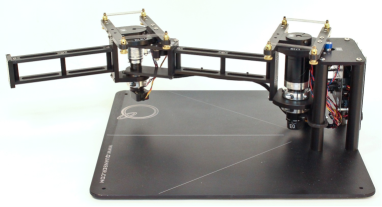
Figure 2: Quanser 2 degrees of freedom serial flexible joints robot manipulator.

For the FJR in Figure 2 we have that $n_{\ell}=n_{m}=2$ in (39), and its parameters are shown in Table 1:

Parameter	Value	Parameter	Value	Parameter	Value
$m_{\ell 1}$	$1.510kg$	$I_{\ell 1}$	$0.0392kg\cdot m^{2}$	$\ell_{\ell 1}$	$0.343m$
$m_{\ell 2}$	$0.873kg$	$I_{\ell 2}$	$0.00808kg\cdot m^{2}$	$\ell_{\ell 2}$	$0.267m$
$m_{m1}$	$0.23kg$	$r_{\ell 1}$	$0.159m$	$D_{\ell}$	diag$\{0.8,0.55\}N\cdot s/m$
$m_{m2}$	$0.01kg$	$r_{\ell 2}$	$0.055m$	$D_{m}$	diag$\{0.2,90\}N\cdot s/m$

Table 1: The parameter values of Quanser FJR as shown in Figure 2

The links and motor inertia matrices are

$$M_{\ell}(q_{\ell})=\begin{bmatrix}a_{1}+a_{2}+2b\cos(q_{\ell 2})&a_{2}+b\cos(q_{\ell 2})\\ a_{2}+b\cos(q_{\ell 2})&a_{2}\end{bmatrix}\quad\text{and}\quad M_{m}(q_{m})=\begin{bmatrix}m_{m1}&0_{n_{m}}\\ 0_{n_{m}}&m_{m2}\end{bmatrix},$$ (73)

respectively; with $a_{1}=m_{\ell 1}r_{\ell 1}^{2}+m_{\ell 2}\ell_{\ell 1}^{2}+I_{\ell 1},a_{2}=m_{\ell 2}r_{\ell 2}^{2}+I_{\ell 2},b=m_{\ell 2}\ell_{\ell 1}r_{\ell 2}$. The workless forces matrix (40) is

$$E(x)=b\sin(q_{\ell 2})\begin{bmatrix}\dot{q}_{\ell 2}&-\dot{q}_{\ell 1}&0_{n_{m}}&0_{n_{m}}\\ \left(\dot{q}_{\ell 1}+\dot{q}_{\ell 2}\right)&0_{n_{\ell}}&0_{n_{m}}&0_{n_{m}}\\ 0_{n_{\ell}}&0_{n_{\ell}}&0_{n_{m}}&0_{n_{m}}\\ 0_{n_{\ell}}&0_{n_{\ell}}&0_{n_{m}}&0_{n_{m}}\\ \end{bmatrix}_{\dot{q}=M^{-1}(q)p},$$ (74)

whose structure’s block matrices are explicitly given by

$$S_{\ell}=b\sin(q_{\ell 2})\begin{bmatrix}0_{n_{\ell}}&-\dot{q}_{\ell 1}-0.5\dot{q}_{\ell 2}\\ \dot{q}_{\ell 1}+0.5\dot{q}_{\ell 2}&0_{n_{\ell}}\end{bmatrix},\dot{M}_{\ell}=-b\sin(q_{\ell 2})\begin{bmatrix}2\dot{q}_{\ell 2}&\dot{q}_{\ell 2}\\ \dot{q}_{\ell 2}&0_{n_{\ell}}\end{bmatrix},S_{m}=\begin{bmatrix}0_{n_{m}}&0_{n_{m}}\\ 0_{n_{m}}&0_{n_{m}}\end{bmatrix},\dot{M}_{m}=\begin{bmatrix}0_{n_{m}}&0_{n_{m}}\\ 0_{n_{m}}&0_{n_{m}}\end{bmatrix}.$$ (75)

5.2 A saturated-type $(\Lambda,K_{d},\phi_{1}(\tilde{q}_{v}))$-controller

This scheme is an example of Corollary 4.5 where only the pH-like variational structure in (35) is preserved in the closed-loop. Let us introduce the following operators for given vector $w\in\mathds{R}^{p}$ as

$$\text{Tanh}(w):=\begin{bmatrix}\text{tanh}(w_{1}),\\ \vdots\\ \text{tanh}(w_{p})\end{bmatrix}\in\mathds{R}^{p}\quad\quad\text{and}\quad\quad\text{SECH}(w)=\begin{bmatrix}\text{sech}(w_{1})&\cdots&0\\ \vdots&\ddots&\vdots\\ 0&\cdots&\text{sech}(w_{p})\end{bmatrix}\in\mathds{R}^{p\times p}.$$ (76)

5.2.1 Controller construction

Since conditions on $\Pi_{q}$ and $K_{d}$ are already given, the constructive procedure is reduced to finding $\phi_{\ell}(\tilde{q}_{\ell v})$ and $\phi_{m}(\tilde{q}_{mv})$ such that inequalities in (44) and (52) hold simultaneously, or equivalently a function $\phi_{1}(\tilde{q}_{v})=[\phi_{\ell}^{\top}(\tilde{q}_{\ell v}),\phi_{m}^{\top}(\tilde{q}_{mv})]^{\top}$ such that

$$-\Lambda\frac{\partial\phi_{1}}{\partial\tilde{q}_{v}}(\tilde{q}_{v})-\frac{\partial\phi_{1}^{\top}}{\partial\tilde{q}_{v}}(\tilde{q}_{v})\Lambda\leq-2\beta_{\tilde{q}}\Lambda.$$ (77)

Corollary 5.1.

Consider $\phi_{1}(\tilde{q}_{v}):=\Lambda\text{Tanh}(\tilde{q}_{v})$. Then, hypotheses in Corollary 4.5 hold and inequality (77) is satisfied with

$$\beta_{\tilde{q}}=\frac{\lambda_{\min}(\Lambda^{2})\cdot\lambda_{\min}(\text{SECH}^{2}(\tilde{q}_{v}))}{\lambda_{\max}(\Lambda)},$$ (78)

where $\lambda_{\min}(\cdot)$ and $\lambda_{\max}(\cdot)$ are the minimum and maximum eigenvalue of their matrix argument, respectively.

Notice that despite the pH-like structure of (33) is not preserved, the vector field $\phi_{1}(\tilde{q}_{v})$ is a conservative vector field. Indeed,

$$P_{v}(\tilde{q}_{v})=\int_{0}^{\tilde{q}_{v}}\Lambda\text{Tanh}(\xi)d\xi=\sum_{k=1}^{n_{\ell}}\lambda_{k}\ln(\cosh(\tilde{q}_{\ell v,k}))+\sum_{k=1}^{n_{m}}\lambda_{k}\ln(\cosh(\tilde{q}_{mv,k})).$$ (79)

This scalar function can be interpreted as the true potential energy when constrained to the manifold $\sigma_{v}=0_{n}$.

Remark 5.2.

The range of $\text{sech}(\cdot)$ is $(0,1]$. Then, it implies that $\phi_{2}(\tilde{q}_{v})=\Lambda\tilde{q}_{v}$ also satisfies inequalities in (44) and (52) with

$$\beta_{\tilde{q}}=\frac{\lambda_{min}(\Lambda^{2})}{\lambda_{max}(\Lambda)}.$$ (80)

With $\phi_{2}(\tilde{q}_{v})=\Lambda\tilde{q}_{v}$ condition (60) holds and the pH-like form (33) is preserved, where the Hamiltonian function in (62) is

$$\tilde{H}_{v}(\tilde{x}_{v},{x})=\frac{1}{2}\tilde{q}^{\top}\Lambda\tilde{q}+\frac{1}{2}\sigma^{\top}M^{-1}(q)\sigma.$$ (81)

Hence, the scheme with $\phi_{2}(\tilde{q}_{v})$ is a structure preserving passivity-based controller for the original FJR. This controller is in fact the example presented in our preliminary conference work in Reyes-Báez ¹⁹, and the generalization to the FJRs case of the tracking scheme for fully-actuated rigid robots developed in Reyes-Báez²⁰.

5.2.2 Experimental results

The experimental results of the robot of Figure 2 in closed-loop system with this saturated-type $(\Lambda,K_{d},\phi_{1}(\tilde{q}_{v}))$-controller are shown in Figure 3. The gain matrices are $\Lambda_{\ell}=\text{diag}\{55,30\}$, $\Lambda_{m}=\text{diag}\{70,60\}$, $K_{\ell d}=\text{diag}\{15,10\}$ and $K_{md}=\text{diag}\{10,5\}$.
On the two upper figures, the time response of ${q}$ and $\tilde{q}_{m}$ is shown. On the left upper plot ${q}_{\ell}$ and $q_{m}$ are compared with the desired trajectory $q_{\ell d}$; it can be seen that links and motors positions indeed converge to $q_{\ell d}$, but only practically due to there are steady-state errors. These offsets in the state variables are attributed to the noise induced by the numerical computation of higher order derivatives. These can be better observed in the upper right plot, where the error variables are shown.
On the lower left plot of Figure 3, similarly, we observe that the time response of the momentum error variables also converge practically to zero and there is noise in the signals. As said before, the main reason is that the velocity (and hence the momentum) are computed numerically through a filter block in Simulink which causes some noise.
Even though the family of controllers of Proposition 4.2 requires the computation of the second and third derivatives of $q_{\ell}$ due to the definition of $p_{mr}$ in (51), we were able to implement controller without them by employing directly the dynamical equations in (39). In fact, the control signals are shown in the right-lower plot in Figure 2.

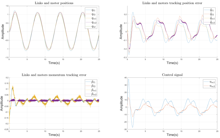
Figure 3: Closed-loop trajectories and control signal with the saturated-type $(\Lambda,K_{d},\phi_{1}(\tilde{q}_{v}))$-controller.

5.3 A v-CBC $(\Lambda,K_{d},\phi_{3}(\cdot))$-controller via the matrix measure $\mu_{1}$

By exploiting the equivalence relation between condition (10) in the direct differential Lyapunov method of Theorem 2.1 and its counterpart for generalized Jacobian in (13) in terms of matrix measures, we propose an alternative constructive procedure for $\phi_{\ell}(\tilde{q}_{\ell v})$ and $\phi_{m}(\tilde{q}_{mv})$ such that conditions (44) and (52) are both satisfied. In this specific case, we consider the matrix measure associated to the $\|\Theta x\|_{1}$ norm for a given matrices $\Theta,A\in\mathds{R}^{p\times p}$ defined as³⁶

$$\mu_{1}(A):=\max_{j}\left(A_{jj}(\tilde{q}_{v},t)+\sum_{i\neq j}|A_{ij}(\tilde{q}_{v},t)|\right).$$ (82)

5.3.1 Controller construction

The generalized Jacobian for $\phi_{3}(\tilde{q}_{v})=[\phi_{\ell}^{\top}(\tilde{q}_{\ell v}),\phi_{m}^{\top}(\tilde{q}_{mv})]^{\top}$ in this case is

$$\overline{J}(\tilde{q}_{v},t)=\Theta\frac{\partial\phi_{3}}{\partial\tilde{q}_{v}}(\tilde{q}_{v})\Theta^{-1}=\begin{bmatrix}-\frac{\partial\phi_{\ell 1}}{\partial\tilde{q}_{\ell v1}}(\tilde{q}_{\ell v})&-\frac{\theta_{1}}{\theta_{2}}\frac{\partial\phi_{\ell 1}}{\partial\tilde{q}_{\ell v2}}(\tilde{q}_{\ell v})&0_{n_{\ell}}&0_{n_{\ell}}\\ -\frac{\theta_{2}}{\theta_{1}}\frac{\partial\phi_{\ell 2}}{\partial\tilde{q}_{\ell v1}}(\tilde{q}_{\ell v})&-\frac{\partial\phi_{\ell 2}}{\partial\tilde{q}_{\ell v2}}(\tilde{q}_{\ell v})&0_{n_{\ell}}&0_{n_{\ell}}\\ 0_{m}&0_{m}&-\frac{\partial\phi_{m1}}{\partial\tilde{q}_{mv1}}(\tilde{q}_{mv})&-\frac{\theta_{3}}{\theta_{4}}\frac{\partial\phi_{m1}}{\partial\tilde{q}_{mv2}}(\tilde{q}_{mv})\\ 0_{m}&0_{m}&-\frac{\theta_{4}}{\theta_{3}}\frac{\partial\phi_{m2}}{\partial\tilde{q}_{mv1}}(\tilde{q}_{mv})&-\frac{\partial\phi_{m2}}{\partial\tilde{q}_{mv2}}(\tilde{q}_{mv})\end{bmatrix},$$ (83)

where $\Lambda=\Theta^{\top}\Theta$ for matrix $\Theta=\text{diag}\{\theta_{1},\theta_{2},\theta_{3},\theta_{4}\}>0_{n}$, and matrix measure is explicitly given by

$$\begin{split}\mu_{1}(\overline{J})=\max\left\{-\frac{\partial\phi_{\ell 1}}{\partial\tilde{q}_{\ell v1}}+\bigg{|}\frac{\theta_{2}}{\theta_{1}}\frac{\partial\phi_{\ell 2}}{\partial\tilde{q}_{\ell v1}}\bigg{|},-\frac{\partial\phi_{\ell 2}}{\partial\tilde{q}_{\ell v2}}+\bigg{|}\frac{\theta_{1}}{\theta_{2}}\frac{\partial\phi_{\ell 1}}{\partial\tilde{q}_{\ell v2}}\bigg{|},-\frac{\partial\phi_{m1}}{\partial\tilde{q}_{mv1}}+\bigg{|}\frac{\theta_{4}}{\theta_{3}}\frac{\partial\phi_{m2}}{\partial\tilde{q}_{mlv1}}\bigg{|},-\frac{\partial\phi_{m2}}{\partial\tilde{q}_{mv2}}+\bigg{|}\frac{\theta_{3}}{\theta_{4}}\frac{\partial\phi_{m1}}{\partial\tilde{q}_{mv2}}\bigg{|}\right\}.\end{split}$$ (84)

Thus, the contractivity condition in (77) is equivalent to

$$\mu_{1}(\overline{J}(\tilde{q}_{v},t))\leq-2\beta_{\tilde{q}_{v}},$$ (85)

where $2\beta_{\tilde{q}_{v}}:=\min\{c_{1}^{2},c_{2}^{2},c_{3}^{2},c_{4}^{2}\}$, with $c_{1},c_{2},c_{3},c_{4}$ positive constants satisfying the following inequalities

$$\begin{split}\overline{J}_{11}(\tilde{q}_{v})+|\overline{J}_{21}(\tilde{q}_{v})|<-c_{1}^{2};\quad\overline{J}_{22}+|\overline{J}_{12}|<-c_{2}^{2};\quad\overline{J}_{33}(\tilde{q}_{v})+|\overline{J}_{43}(\tilde{q}_{v})|<-c_{3}^{2};\quad\overline{J}_{44}+|\overline{J}_{34}|<-c_{4}^{2}.\end{split}$$ (86)

Corollary 5.3.

Let $\phi_{3}(\tilde{q}_{v})$ be defined by

$$\phi_{3}(\tilde{q}_{v})=\begin{bmatrix}\phi_{\ell 1}(\tilde{q}_{\ell v})\\ \phi_{\ell 2}(\tilde{q}_{\ell v})\\ \phi_{m1}(\tilde{q}_{mv})\\ \phi_{m2}(\tilde{q}_{mv})\end{bmatrix}=\begin{bmatrix}(1+\kappa_{1})\tilde{q}_{\ell v1}+\frac{\theta_{2}}{\theta_{1}}\text{tanh}(\tilde{q}_{\ell v2})\\ \frac{\theta_{1}}{\theta_{2}}\text{tanh}(\tilde{q}_{\ell v1})+(1+\kappa_{2})\tilde{q}_{\ell v2}\\ (1+\kappa_{3})\tilde{q}_{mv1}+\frac{\theta_{4}}{\theta_{3}}\text{tanh}(\tilde{q}_{mv2})\\ \frac{\theta_{3}}{\theta_{4}}\text{tanh}(\tilde{q}_{mv1})+(1+\kappa_{4})\tilde{q}_{mv2}\end{bmatrix},$$ (87)

where $\kappa_{1},\kappa_{2},\kappa_{3},\kappa_{4}$ are strictly positive constants. Then, condition (85) is satisfied with $c_{1}^{2}=\kappa_{1},c_{2}^{2}=\kappa_{2},c_{3}^{2}=\kappa_{3}$ and $c_{4}^{2}=\kappa_{4}$ .

With this scheme neither the structure of (33) nor the variational one of (35) are preserved. Nevertheless, uniform global exponential convergence to $q_{\ell d}$ is still guarantee. Interestingly, in this scheme the convergence rate $\beta_{\tilde{q}_{v}}$ does not depend on gain $\Lambda$, which give extra freedom in the tuning process. In particular, when constrained to the manifold $\sigma_{v}=0_{n}$, the convergence to $q_{\ell d}$ can be accelerated by the gain $\kappa_{i},i\in\{1,\dots,4\}$.

5.3.2 Experimental results

For the experiment with this controller, we consider the following specifications: $\kappa_{1}=10,\kappa_{2}=8$, $\theta_{1}=\sqrt{\Lambda_{\ell,11}}$, $\theta_{2}=\sqrt{\Lambda_{\ell,22}}$, $\theta_{3}=\sqrt{\Lambda_{m,11}}$ and $\theta_{4}=\sqrt{\Lambda_{m,22}}$ with the same gain matrices $\Lambda_{\ell}$, $\Lambda_{m}$, $K_{\ell d}$ and $K_{md}$ of the previous experiment.
The closed-loop time response is shown in Figure 4. At first stage we can observe that the performance with respect to the previous controller is improved; this is mainly attributed to the gains $\kappa_{i},i\in\{1,\dots,4\}$.
Indeed, on the left upper plot we can see how the links and motors positions almost superimpose the desired links trajectory $q_{\ell d}$. This can be appreciated better on the upper-right plot where the error variables are shown; we observe that we still have only practical convergence since there is steady-state errors, but these are considerably reduced with respect to the precious scheme as well as the overshoot in the transient time interval. We also observe some noise in the motors positions.
On the left lower plot we see the time response of the momentum error variables which have considerably decreased with respect to the previous controller. In fact, as it may be expected the overshoot during the transient time has decreased as well as the steady state momentum errors which amplitudes, excepting $\tilde{p}_{m1}$, is of the order of $10^{-2}$. Here we still have the noise problem due to the numerical computation of the momentum feedback, and in this case also the control effort of the links dynamics.
On the right lower plot, we see that the overshoot of the control signals has increased but steady-state signals amplitude is more less the same but with a rms value added. This is the expected price to pay after adding an extra control gain.

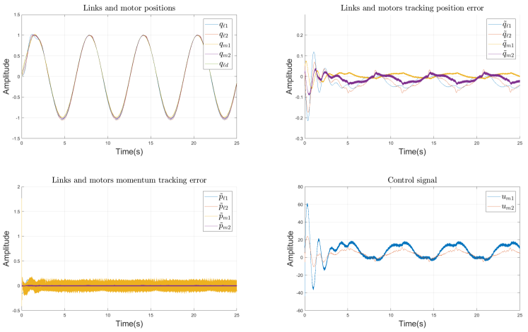
Figure 4: Closed-loop trajectories and control signal with the $(\Lambda,K_{d},\phi_{1}(\tilde{q}_{v}))$-controller via the matrix measure $\mu_{1}$.

6 Conclusions

In this work we have proposed a large family of virtual-contraction based controllers that solve the standard trajectory tracking problem of FJRs modeled as port-Hamiltonian systems. With these controllers, global exponential convergence to a predefined reference trajectory is guaranteed. The design procedure is based on the notions of contractivity and virtual systems.

The developed family of v-CBC are PD-like controllers which have three design "parameters" that give different structural properties to the closed-loop virtual system like pH-like structure preserving, variational pH-like structure preserving, differential passivity, among others. These properties were used for constructing two novel nonlinear PD-like v-CBC schemes. The performance of the aforementioned controllers was evaluated experimentally using the planar flexible-joints robot of two degrees of freedom by from Quanser.

References

• 1 Nicosia S, Tomei P. A tracking controller for flexible joint robots using only link position feedback. IEEE Transactions on Automatic Control. 1995;40(5).
• 2 Spong M W. Modeling and control of elastic joint robots. Journal of dynamic systems, measurement, and control. 1987;109(4):310–319.
• 3 Canudas de Wit C, Siciliano B, Bastin G. Theory of robot control. Springer Science & Business Media; 2012.
• 4 Loria A, Ortega R. On tracking control of rigid and flexible joints robots. Appl. Math. Comput. Sci. 1995;5(2):101–113.
• 5 Ailon A, Ortega R. An observer-based set-point controller for robot manipulators with flexible joints. Systems & Control Letters. 1993;21(4):329 - 335.
• 6 Brogliato B, Ortega R, Lozano R. Global tracking controllers for flexible-joint manipulators: a comparative study. Automatica. 1995;31(7):941–956.
• 7 Ortega R, Perez J A, Nicklasson P J, Sira-Ramirez H. Passivity-based control of Euler-Lagrange systems. Springer Science & Business Media; 2013.
• 8 Astolfi A, Ortega R. Immersion and invariance: A new tool for stabilization and adaptive control of nonlinear systems. IEEE Transactions on Automatic control. 2003;48(4):590–606.
• 9 Albu-Schäffer A, Ott C, Hirzinger G. A unified passivity-based control framework for position, torque and impedance control of flexible joint robots. The international journal of robotics research. 2007;26(1).
• 10 Avila-Becerril S, Lorá A, Panteley E. Global position-feedback tracking control of flexible-joint robots. Paper presented at: American Control Conference (ACC), 2016. 2016; Boston, MA, USA;:3008–3013.
• 11 Pan Yongping, Wang Huiming, Li Xiang, Yu Haoyong. Adaptive command-filtered backstepping control of robot arms with compliant actuators. IEEE Transactions on Control Systems Technology. 2017;26(3):1149–1156.
• 12 van der Schaft A J, Maschke B M. The Hamiltonian formulation of energy conserving physical systems with external ports. Archiv für Elektronik und Übertragungstechnik. 1995;49.
• 13 Ortega R, Borja L P. New results on control by interconnection and energy-balancing passivity-based control of port-Hamiltonian systems. Paper presented at: Decision and Control (CDC), IEEE 53rd Annual Conference on. 2014;:2346–2351.
• 14 Ortega R, van der Schaft A J, Castaños F, Astolfi A. Control by interconnection and standard passivity-based control of port-Hamiltonian systems. IEEE Transactions on Automatic Control. 2008;53.
• 15 Zhang Q, Xie Z, Kui S, Yang H, Minghe J, Cai H. Interconnection and damping assignment passivity-based control for flexible joint robot. Paper presented at: Intelligent Control and Automation (WCICA), 11th World Congress on Intelligent Control and Automation. 2014;:4242–4249.
• 16 Ortega R, van der Schaft A J, Maschke B, Escobar G. Interconnection and damping assignment passivity-based control of port-controlled Hamiltonian systems. Automatica. 2002;38(4):585–596.
• 17 Jayawardhana B. Tracking and Disturbance Rejection of Passive Nonlinear Systems. Ph.D. thesis, Imperial College London; 2006.
• 18 Jardón-Kojakhmetov H, Munoz-Arias M, Scherpen J M A. Model reduction of a flexible-joint robot: a port-Hamiltonian approach. IFAC-PapersOnLine. 2016;49(18):832 - 837. 10th IFAC Symposium on Nonlinear Control Systems NOLCOS.
• 19 Reyes-Báez R, van der Schaft A J, Jayawardhana B. Virtual Differential Passivity based Control for Tracking of Flexible-joints Robots. IFAC-PapersOnLine. 2018;51(3):169 - 174. 6th IFAC Workshop on Lagrangian and Hamiltonian Methods for Nonlinear Control LHMNC.
• 20 Reyes-Báez R, van der Schaft A J, Jayawardhana B. Tracking Control of Fully-actuated port-Hamiltonian Mechanical Systems via Sliding Manifolds and Contraction Analysis. IFAC-PapersOnLine. 2017;50(1):8256 - 8261. 20th IFAC World Congress.
• 21 Reyes-Báez R, van der Schaft A J, Jayawardhana B. Virtual differential passivity based control for a class of mechanical systems in the port-Hamiltonian framework. Submitted. 2018;.
• 22 Forni F, Sepulchre R. A Differential Lyapunov Framework for Contraction Analysis. IEEE Transactions on Automatic Control. 2014;.
• 23 Pavlov A, van de Wouw Nathan. Convergent systems: nonlinear simplicity. In: Springer 2017 (pp. 51–77).
• 24 Lohmiller W, Slotine J J E. On contraction analysis for non-linear systems. Automatica. 1998;.
• 25 Sontag E D. Contractive systems with inputs. In: Springer 2010 (pp. 217–228).
• 26 Wang W, Slotine J J E. On partial contraction analysis for coupled nonlinear oscillators. Biological cybernetics. 2005;92(1).
• 27 Jouffroy J, Fossen T. A tutorial on incremental stability analysis using contraction theory. Modeling, Identification and control. 2010;31(3):93–106.
• 28 Manchester I R, Tang J Z, Slotine J J E. Unifying classical and optimization-based methods for robot tracking control with control contraction metrics. Paper presented at: International Symposium on Robotics Research (ISRR). 2015;:1–16.
• 29 Angeli D. A Lyapunov approach to incremental stability properties. IEEE Transactions on Automatic Control. 2002;47(3):410–421.
• 30 van der Schaft A J. On differential passivity. IFAC Proceedings Volumes. 2013;46(23):21–25. 9th IFAC Symposium on Nonlinear Control Systems.
• 31 Reyes Báez Rodolfo. Virtual contraction and passivity based control of nonlinear mechanical systems: trajectory tracking and group coordination. PhD thesisUniversity of Groningen2019.
• 32 Khalil H K. Noninear systems. Prentice-Hall, New Jersey. 1996;2(5):5–1.
• 33 Crouch PE, van der Schaft AJ. Variational and Hamiltonian Control Systems. Springer-Verlag. 1987;.
• 34 Sanfelice R G, Praly L. Convergence of nonlinear observers on $\mathds{R}^{n}$ with a Riemannian metric (part I). IEEE Transactions on Automatic Control. 2015;.
• 35 Coogan S. A Contractive Approach to Separable Lyapunov Functions for Monotone Systems. arXiv preprint arXiv:1704.04218. 2017;.
• 36 Russo G, Di Bernardo M, Sontag E D. Global entrainment of transcriptional systems to periodic inputs. PLoS computational biology. 2010;6(4):e1000739.
• 37 Forni F, Sepulchre R. On differentially dissipative dynamical systems. IFAC Proceedings Volumes. 2013;46(23):15 - 20. 9th IFAC Symposium on Nonlinear Control Systems.
• 38 Forni F, Sepulchre R, van der Schaft A J. On differential passivity of physical systems. In: :6580–6585IEEE; 2013.
• 39 Arimoto S, Miyazaki F. Stabilidty and robustness of PID feedback control for robot manipulators of sensory capability. Robotics Research, The 1st Symp., by M Brady & R.P. Paul, Eds., MIT Press, Cabridge Massachusetts. 1984;.
• 40 Ott C, Albu-Schaffer A, Kugi A, Hirzinger G. On the passivity-based impedance control of flexible joint robots. IEEE Transactions on Robotics. 2008;24(2):416–429.
• 41 van der Schaft A J, Jeltsema D. Port-Hamiltonian systems theory: An introductory overview. Foundations and Trends in Systems and Control. 2014;1.
• 42 Pavlov A, Marconi L. Incremental passivity and output regulation. Paper presented at: IEEE Conference on Decision and Control. 2006;.
• 43 Kawano Y, Ohtsuka T. Nonlinear Eigenvalue Approach to Differential Riccati Equations for Contraction Analysis. IEEE Transactions on Automatic Control. 2017;62(12):6497-6504.
• 44 Quanser Consulting Inc. 2-DOF serial flexible link robot, Reference Manual, Doc. No. 763, Rev. 1, 2008.