The utilization of total mass to determine the switching points in the symmetric boundary control of a diffusion problem
M. Salman
Department of Math, Physics & Stat,
Qatar University, PO Box 2713, Doha, Qatar
msalmanz@gmail.com
Abstract.
The authors study the problem and where for
and for with and the sequence is
determined by the equations for
and for
and where . Note that the switching
points are unknown. Existence and
uniqueness are demonstrated. Theoretical estimates of the
and are obtained and numerical verifications of the
estimates are presented.
1. Introduction
As motivation for the mathematical problems considered
in this work, consider a chamber in the form of a long linear
transparent tube. We allow for the introduction or removal of
material in a gaseous state at the ends of the tube. The material
diffuses throughout the tube with or without reaction with other
materials. By illuminating the tube on one side with a light source
with a frequency range spanning the absorption range for the
material and collecting the residual light that passes through the
tube with photo-reception equipment, we can obtain a measurement of
the total mass of material contained in the tube as a function of
time. Using the total mass as switch points for changing the
boundary conditions for introduction or removal of material. The
objective is to keep the total mass of material in the tube
oscillating between two set values such as . The physical
application for such a system is the control of reaction diffusion
systems such as production of a chemical material in a reaction
chamber via the introduction of reactants at the boundary of
chamber.
In this work we study the diffusion equation
(1.1)
subject to the initial
concentration
and boundary conditions controlled by the total mass . We are going to begin by setting the
concentration to be at both boundary points and
, where is a positive constant. We shall watch the
total mass until it reaches a certain
specified level at time , where . At this
moment, we switch the concentration to
We keep watching the total mass until it drops down to a
prespecified level at time , where . We keep
switching the concentration according to the level of the total
mass so that we always have
In other words, the boundary conditions will be
(1.2)
where
; and the sequence will be strictly
increasing, i.e.
and its terms are defined by the equations
2. Existence of the Sequence
For the sake of simplicity, we will take . Consider the
problem
Using a similar
argument, we can inductively obtain
(3.7)
Next we use mathematical induction to prove (3.7). The point
can be obtained by
Assuming formula (3.7) is valid for all , then the
last equation is equivalent to
Upon adding all the terms inside the brackets as a finite
geometric sum, we will obtain
(3.8)
The time
step can be found as a solution of
Assuming the validity of (3.7) and using (3.8) for
all , the above equation implies
If we add these terms which constitute finite geometric series, we
can obtain
(3.9)
Hence, formula (3.7)
is valid.
Formula (3.7) implies that
Therefore,
which is obviously independent of .
4. A Higher Order Approximation
In this section we will study a higher order approximation of the
sequence . This approximation is based on dropping all
the terms that has from the expression
of the mass, except for a few dominating terms. The upper and
lower bounds on the mass are not necessarily symmetric. For
simplicity of computation, the bounds are chosen to be
and
where ; and
are positive numbers that are chosen so that the inequality
holds. Since , then we have
.
To find , we need to solve the
equation
which is
Upon dropping all the terms that have for
all , we get
which implies
(4.1)
In a
similar fashion, we compute by solving
i.e.,
By dropping all the terms that have for all
, we get
Using (4.1) we obtain
(4.2)
By employing a similar method of approximations we can find
through the equation
which implies that
(4.3)
For and , we obtain the explicit
expressions
(4.4)
and
(4.5)
Thus, we choose
(4.6)
and
(4.7)
By an induction argument similar to the one used in Section 3
we can show that (4.6) and (4.7) hold. Therefore the consecutive
time steps can be calculated by
(4.8)
and
(4.9)
where . For the special case
when , the time intervals reduce that shown at the end
of section 3.
5. Numerical Results
In this section, we use a finite difference technique along with
the trapezoidal rule to get an approximate discrete solution
and the sequence when the total mass hits one
of the limits or .
We discretize the space and time by using
i)
ii)
where and are positive integer and is a
positive real number. The integer has to be chosen large
enough so that the time step is much smaller than the
differences .
We consider the backward implicit finite difference scheme
as a discretized version of , where is a positive
constant. The above scheme can be written in the form
(5.1)
where
and . The initial data are set to
be for , and the boundary conditions are
for . The function
will be either 10 or 0 depending on the value of
the mass which will be approximated by the trapezoidal rule
(5.2)
The numerical experiment is carried out in the
following way. We start by setting the boundary conditions
then we solve a tridiagonal system coming out of
the difference method. We check the total mass in (5.2). We
keep doing that at each time step until the mass exceeds or
equals the upper limit . Then we switch the boundary conditions
to , and we continue the finite difference scheme for
several time steps until the total mass decreases
to . At this moment we switch the boundary condition back to 10
and continue the process as we did before.
For the data specifications , ,
, , , Table (1) shows the times switches .
As we can see there, the duration of each stage
turns out to be constant.
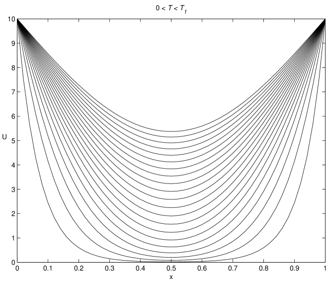
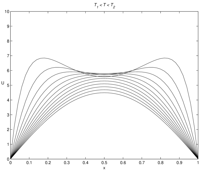
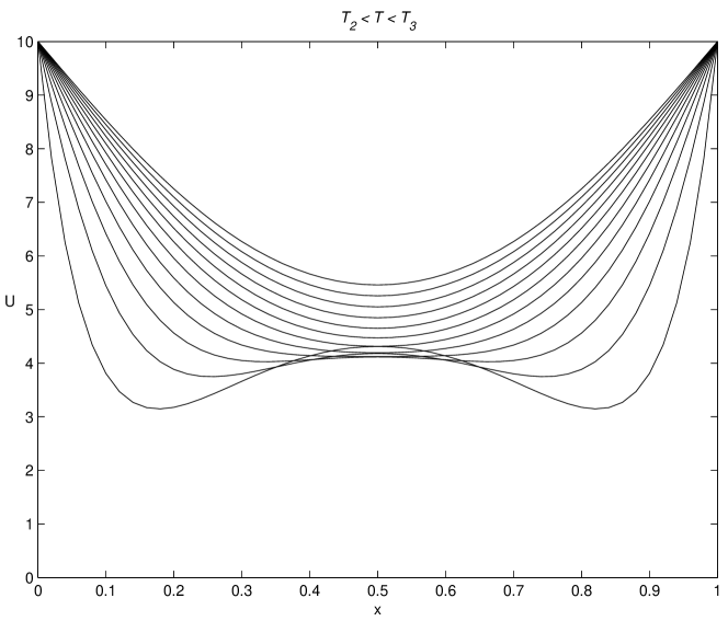
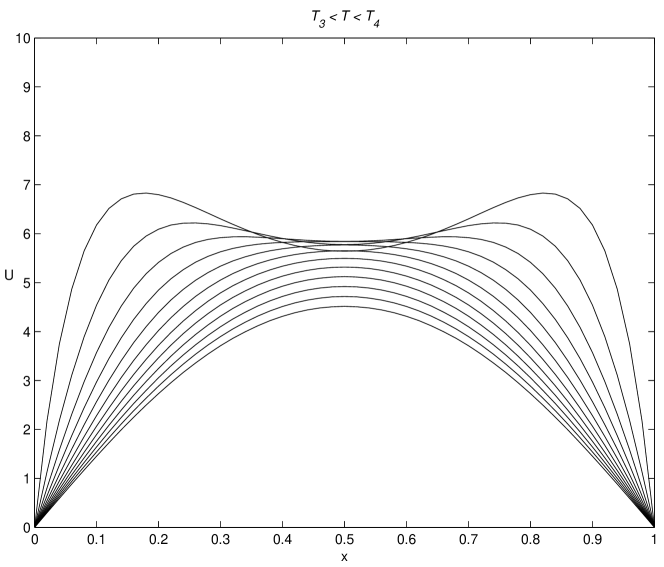
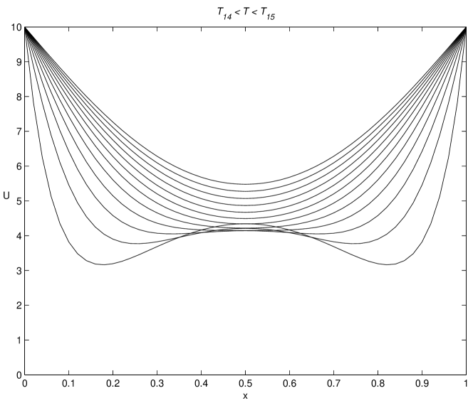
For the same set of data, Graphs (1) through (6) show the
concentration versus the space. The graphs are obtained for
different stages, where at each stage the concentration is kept
constant at the end points.
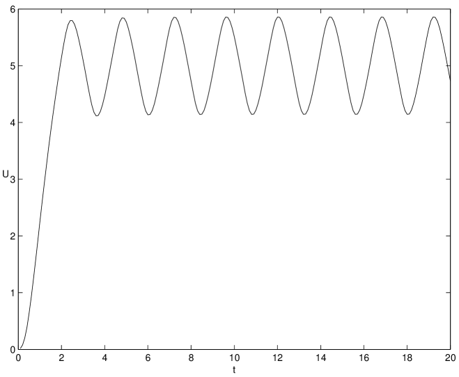
A profile of the concentrations at for various times is shown
in Graph (7) with the same specified data.
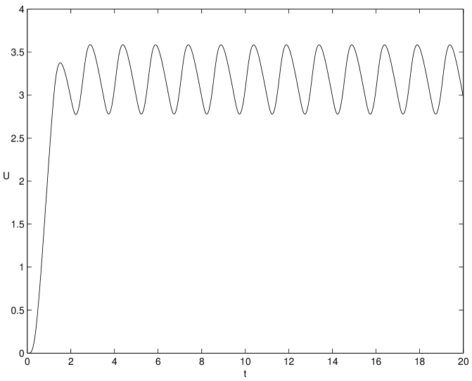
For a different set of upper and lower bounds on the mass
and along with , ,
Table (2) shows the time switches . Durations of the
time intervals fluctuates between 0.5, 1.
Graph (8) is the concentration at for the same data
generating Table (2).
Conclusion: From Table 1 and
Table 2, we see that the theoretical estimates of
and are exihibited in the
numerical examples.
n
Tn
Tn - Tn-1
n
Tn
Tn - Tn-1
1
2.1000
2.1000
8
10.5000
1.2000
2
3.3000
1.2000
9
11.7000
1.2000
3
4.5000
1.2000
10
12.9000
1.2000
4
5.7000
1.2000
11
14.1000
1.2000
5
6.9000
1.2000
12
15.3000
1.2000
6
8.1000
1.2000
13
16.5000
1.2000
7
9.3000
1.2000
14
17.7000
1.2000
Table 1. Time switches corresponding to ,
, , , ,
n
Tn
Tn - Tn-1
n
Tn
Tn - Tn-1
1
1.0000
1.0000
14
10.9400
1.0200
2
1.9400
0.9400
15
11.4200
0.4800
3
2.4200
0.4800
16
12.4400
1.0200
4
3.4400
1.0200
17
12.9200
0.4800
5
3.9200
0.4800
18
13.9400
1.0200
6
4.9400
1.0200
19
14.4200
0.4800
7
5.4200
0.4800
20
15.4400
1.0200
8
6.4400
1.0200
21
15.9200
0.4800
9
6.9200
0.4800
22
16.9400
1.0200
10
7.9400
1.0200
23
17.4200
0.4800
11
8.4200
0.4800
24
18.4400
1.0200
12
9.4400
1.0200
25
18.9200
0.4800
13
9.9200
0.4800
26
19.9400
1.0200
Table 2.
Figure 1. The first
stage where the concentration is held at 10 at the end points.
Each curve shows the concentration profile at various discrete
time steps . As the time goes on, the level of
concentrations gets higher
Figure 2. The second
stage where the concentration is held at 0 at the end points.
As the time goes on, the level of
concentrations, roughly speaking, decreases. Notice the
fluctuations when the concentration is dropped suddenly to 0 at
the beginning of the stage
Figure 3.
Figure 4.
Figure 5.
Figure 6.
Figure 7.
Figure 8.
References
[1] J. R. Cannon, The one-dimensional heat equation,
Encyclopedia of Mathematics and its Applications23
(1984).
[2] J. R. Cannon, Yapping Lin and Shuzhan Xu, Numerical
procedures for the determination of an unknown coefficient in
semi-linear parabolic differential equation. Inverse
Problems10 (1994), 227-243.
[3] W. A. Day, Existence of a property of solutions of
the heat equation to linear thermoelasticity and other theories.
Quart. Appl. Math., 40, (1982) 319-330.
[4] W. A. Day, A decreasing property of solutions of
a parabolic equation with applications to thermoelasticity. Quart. Appl. Math., 41, (1983) 468-4475.
[5] J.R. Cannon and J. Van der Hoek, The existence and
a continuous dependance result for the solution of the heat
equation subject to the specification of energy. Boll. Uni.
Math. Ital. Suppl. bf 1(1981), 253-282.
[6] J.R. Cannon and J. Van der Hoek, An emplicit
finite difference scheme for the diffusion of mass in a portion of
a domain. Numerical Solutions of Partial Differential
Equations. (J. Noye, ed) ,527-539, North-Holland,
Amsterdam, 1982.
[7] J.R. Cannon and J. Van der Hoek, Diffusion subject
to a specification of mass. J. Math. Anal. Appl.115
(1986), No.2, 517-529
[8] J. Kevorkian, Partial differential equations, analytical solution techniques. 2nd edition. Texts in Applied Mathematics35 (2000).
[9] Pao, C. V. Blowing-up of solution for a nonlocal reaction-diffusion problem in combustion theory. J. Math. Anal. Appl.166 (1992), no. 2, 591-600.
[10] Pao, C. V. Dynamics of reaction-diffusion equations with nonlocal boundary conditions. Quart. Appl. Math.53 (1995), no. 1, 173-186.
[11] Pao, C. V. Reaction diffusion equations with nonlocal boundary and nonlocal initial conditions. J. Math. Anal. Appl.195 (1995), no. 3, 702-718.
[12] Pao, C. V. Dynamics of weakly coupled parabolic systems with nonlocal boundary conditions. Advances in nonlinear dynamics, 319-327, Stability Control Theory Methods Appl., 5, Gordon and Breach, Amsterdam, 1997.
[13] Pao, C. V. Asymptotic behavior of solutions of reaction-diffusion equations with nonlocal boundary conditions. Positive solutions of nonlinear problems. J. Comput. Appl. Math.88 (1998), no. 1, 225-238.
[14] Pao, C. V. Numerical solutions of reaction-diffusion equations with nonlocal boundary conditions. J. Comput. Appl. Math.136 (2001), no. 1-2, 227-243.
[15] J. W. Thomas, Numerical partial differential equations, finite difference method. Text in Applied Mathematics22 (1995).