Mean Value of the Quantum Potential and Uncertainty Relations

Abstract

In this work we determine a lower bound to the mean value of the quantum potential for an arbitrary state. Furthermore, we derive a generalized uncertainty relation that is stronger than the Robertson-Schrödinger inequality and hence also stronger than the Heisenberg uncertainty principle. The mean value is then associated to the nonclassical part of the covariances of the momenta operator. This imposes a minimum bound for the nonclassical correlations of momenta and gives a physical characterization of the classical and semiclassical limits of quantum systems. The results obtained primarily for pure states are then generalized for density matrices describing mixed states.

I Introduction

Quantum mechanics defines a formal procedure to consistently quantize dynamical systems. The noncommutability of pairs of operators translates into the well-known uncertainty relations, which is one of the most important kinematic feature of quantum mechanics. However, from a completely different perspective, the debate on interpretation of quantum mechanics frequently focuses on the quantum potential, which seems to have no direct connection with the uncertainty relations due to the lack of an operator definition for it.

In nonrelativistic quantum mechanics, the dynamics is defined by Schrödinger equation that unitarily evolves the wave function. Using a polar form for the wave function, Schrödinger equation turns into two real coupled equations for the phase and the modulus of the wave function. One of them is very similar to a Hamilton-Jacobi equation for the phase but possessing an extra term, dubbed quantum potential ( QP), without a classical analog. The QP is responsible for all distinct quantum effects such as entanglement and tunneling. As such, there has been much attention on its properties and several proposals to interpret its physical meaning.

Among the most popular interpretations is Bohmian mechanics, which is a causal interpretation since it dismisses the collapse of the wave function to describe the measurement process Bohm (1952a, b); Bohm and Hiley (1984); Bohm et al. (1987); Holland (1993); Durr et al. (1995). The probabilistic description appears due to the unknown initial position of the particle which plays the role of a hidden parameter, hence it is an instantiation of a successful hidden-variable quantum theory in the sense that it reproduces all experimental results of canonical quantum theory. The Born rule, which in this scope is called equilibrium distribution, need not be imposed but can be dynamically derived. It can be shown that initial nonequilibrium states relax to equilibrium on a coarse-grained levelValentini (1991); Valentini and Westman (2005); Towler et al. (2012); Efthymiopoulos and Contopoulos (2006); Bennett (2010). It is worth mentioning that the ontological nature of the Bohmian trajectories and the interpretation of the QP have concrete applications in quantum cosmology Falciano et al. (2013); Vitenti et al. (2013, 2014); Pinto-Neto and Fabris (2013) and offer a new approach to semi-classical approximations Struyve (2015); Benseny et al. (2014); Struyve (2019).

In Bohmian mechanics the QP is interpreted as carrying information but has no material support. Other scenarios give completely different physical interpretation to the QP. For instance, in Weyl space Carroll (2007, 2007) it is interpreted as a geometrical object associated to the nonmetricity of the metric tensor, hence a manifestation of non-Euclidean geometry at the microscopic scale Novello et al. (2011); Falciano et al. (2010), while from the point of view of information theory, a connection with nonrelativistic quantum mechanics appears as a principle of minimum Fisher information Frieden and Soffer (1995); Reginatto (1998). The latter constitutes a rare example of a natural connection between QP and uncertainty relations (see Frieden (1988, 1989, 1998); Reginatto (1998); Frieden and Soffer (1995); Hall (2000, 2001); Hall and Reginatto (2002) for details).

In the present work we study the mathematical and physical properties of the mean value of the quantum potential ( MVQP). In contrast to the QP, its mean value satisfies inequalities that can be used to derive generalized uncertainties relations, which are shown to be more restrictive than the Heisenberg uncertainty principle. Furthermore, the MVQP is associated to a parcel of the covariances among all the momenta components, which will be called the nonclassical correlations. Thus, some of our results reproduce part of the Fisher information scenario Frieden and Soffer (1995); Reginatto (1998) but without including any extra hypothesis. We also depart from this perspective when generalizing the results for mixed states directly from the Liouville von-Neumann equation.

Our entire analysis is made within the Copenhagen formalism but since it makes no reference to the collapse of the wave function, it can be straightforwardly generalized to other scenarios as well. For instance, the question of the classical and semiclassical limits is described entirely in terms of the presence of nonclassical correlations in the system.

The paper is organized as follows. In the next section we briefly review the basic equations and fix our notation. In sec. III we derive the generalized uncertainty relations for pure states and in sec. IV we show that the MVQP encodes the nonclassical momenta correlations. In sec. V we generalize our pure state previous results for density matrices describing mixed states. In sec. VI we present several comparisons of our results with the Heisenberg and Robertson-Schrödinger uncertainties. In sec. VII we exemplify with concrete physical systems and in sec. VIII we conclude with final remarks.

II Classical and Quantum Dynamics

In this section we briefly review some basic equations in order to fix our notation used in the rest of the paper. Let $q:=(q_{1},...,q_{n})^{\top}$ and $p:=(p_{1},...,p_{n})^{\top}$ be column vectors of, respectively, the $n$ coordinates and canonically conjugated momenta of a system with $n$ degrees of freedom (DF), which has its evolution governed by the Hamiltonian

$$H(q,p)=\tfrac{1}{2}p\cdot{\bf M}p+q\cdot{\bf C}p+p\cdot\xi_{p}+U(q)\ ,$$ (1)

where $\xi_{p}\in\mathbb{R}^{n}$ is a constant column vector, ${\bf M}={\bf M}^{\top}$ and ${\bf C}$ are $n\times n$ real matrices. The term $U(q)$ is a real function describing any other contribution to the potential energy of the system, such that $H(q,p)$ is the most generic Hamiltonian comprising a quadratic kinetic energy, possibly time-dependent.

Canonical quantum mechanics promote classical variables to operators, hence we have $\hat{q}:=(\hat{q}_{1},...,\hat{q}_{n})^{\dagger}$ and $\hat{p}:=(\hat{p}_{1},...,\hat{p}_{n})^{\dagger}$ two column vectors of, respectively, coordinates and canonically conjugated momenta operators of the system. Considering the position eigenstates of the system, $|q\rangle:=|q_{1}\rangle\otimes...\otimes|q_{n}\rangle$, the momenta matrix elements are

$$\langle q^{\prime}_{j}|\hat{p}_{k}|q_{l}\rangle=-i\hbar\,\delta(q^{\prime}_{j}-q_{l})\,\delta_{jl}\,\delta_{lk}\,\partial_{k},$$ (2)

where $\partial_{k}:=\partial/\partial q_{k}$. Here we will adopt a symmetric quantization scheme, such that the quantized version of Hamiltonian (1) becomes the function of operators

$$H(\hat{q},\hat{p})=\tfrac{1}{2}\hat{p}\cdot{\bf M}\hat{p}+\tfrac{1}{2}\hat{q}\cdot{\bf C}\hat{p}+\tfrac{1}{2}\hat{p}\cdot{\bf C}^{\top}\hat{q}+\hat{p}\cdot\xi_{p}+U(\hat{q})\ .$$ (3)

In nonrelativistic quantum mechanics the evolution is dictated by Schrödinger equation, namely, using the position representation $\psi(q,t):=\langle q|\psi_{t}\rangle$ we have

$$i\hbar\partial_{t}\psi(q,t)=H\left(q,-i\hbar\partial_{q}\right)\psi(q,t),$$ (4)

where $\partial_{q}:=(\partial_{1},...,\partial_{n})^{\top}$. As any complex function, the wave function associated to the state $|\psi_{t}\rangle$ may be written in polar form,

$$\psi(q,t)=\Omega(q,t)\,{\rm e}^{\frac{i}{\hbar}S(q,t)}\ ,$$ (5)

where $\Omega(q,t)=|\psi(q,t)|$ and $S(q,t)=\hbar{\rm Arg}[\psi(q,t)]$. Using the polar decomposition for the wave function in the time-dependent Schrödinger equation (4), one obtain two coupled real equations Holland (1993) as follows. One is the continuity equation

$$\partial_{t}\Omega^{2}+{\partial_{q}}\cdot\mathcal{J}_{q}=0$$ (6)

for the probability density $\Omega^{2}(q,t)=\psi^{\ast}(q,t)\psi(q,t)$ with probability current given by

$$\mathcal{J}_{q} :=\Omega^{2}\,\partial_{p}H\big{|}_{p=\partial_{q}S}=\Omega^{2}\!\left(\xi_{p}+{\bf C}^{\top}q+{\bf M}\partial_{q}S\right)\ ;$$ (7)

the other is like the classical Hamilton-Jacobi equation for the phase $S(q,t)$,

$$\partial_{t}S+H(q,\partial_{q}S)+Q(q,t)=0\ ,$$ (8)

but with an extra term,

$$Q(q,t):=-\frac{\hbar^{2}}{2\Omega}{\partial_{q}}\cdot{\bf M}{\partial_{q}\Omega}\ ,$$ (9)

dubbed the quantum potential (QP), which is a nonlocal potential encoding the information about the state of the system and depends only on $\Omega(q,t)$. Moreover, given its invariance under $\Omega\to k\Omega$ for a constant $k$, we see that the QP does not depend on the strength of $\Omega(q,t)$, but only in its form.

In the presence of any sort of classical randomness, the system state in quantum mechanics should be described by a density operator $\hat{\rho}$, which evolution is governed by the Liouville-von Neumann equation: $i\hbar\,\partial_{t}\hat{\rho}=[\hat{H},\hat{\rho}]$. Taking the position matrix elements of the evolution equation for the Hamiltonian (3), using a position-completeness relation together with (2), it becomes

$$\!\!i\hbar{\partial_{t}}\langle q|\hat{\rho}|{q^{\prime}}\rangle=\left[H\left(q,-{i\hbar}\partial_{q}\right)-H\left(q^{\prime},{i\hbar}\partial_{q^{\prime}}\right)\right]\langle q|\hat{\rho}|{q^{\prime}}\rangle.$$ (10)

Similarly to (5), we will use the polar decomposition

$$\langle q|\hat{\rho}|{q^{\prime}}\rangle=\bar{\Omega}(q,{q^{\prime}},t)\,\exp\!\left[\frac{i}{\hbar}\bar{S}(q,{q^{\prime}},t)\right]\ ,$$ (11)

which, when inserted in (10) for the Hamiltonian (1), give us also two coupled differential equations. A continuity like equation that now reads

$$\partial_{t}\bar{\Omega}^{2}+{\partial_{q}}\cdot\mathcal{J}_{q}+\partial_{q^{\prime}}\cdot\mathcal{J}_{q^{\prime}}=0\ ,$$ (12)

where $\mathcal{J}_{q}$ is exactly written as (7) but replacing $\Omega(q,t)\to\bar{\Omega}(q,q^{\prime},t)$ and $S(q,t)\to\bar{S}(q,q^{\prime},t)$ and the current associated to the $q^{\prime}$ coordinates is

$$\mathcal{J}_{q^{\prime}}:=\bar{\Omega}^{2}\!\left(\xi_{p}+{\bf C}^{\top}{q^{\prime}}-{\bf M}\partial_{q^{\prime}}\bar{S}\right)\ .$$

The other equation is again a kind of Hamilton-Jacobi equation with some extra terms:

$$\partial_{t}\bar{S} +H(q,\partial_{q}\bar{S})-\frac{\hbar^{2}}{2\bar{\Omega}}{\partial_{q}}\cdot\mathbf{M}\partial_{q}\bar{\Omega}\,$$

$$-H(q^{\prime},-\partial_{q^{\prime}}\bar{S})+\frac{\hbar^{2}}{2\bar{\Omega}}\partial_{q^{\prime}}\cdot\mathbf{M}\partial_{q^{\prime}}\bar{\Omega}=0\ .$$ (13)

For a pure state $\hat{\rho}=|\psi_{t}\rangle\!\langle\psi_{t}|$, $\bar{\Omega}(q,q^{\prime},t)=\Omega(q,t)\Omega(q^{\prime},t)$, and $\bar{S}(q,q^{\prime},t)=S(q,t)-S(q^{\prime},t)$. In this circumstance, one can apply a separation of variables into the partial differential equations (12) and (II) to obtain, respectively, two versions of (6) and (8); the separation constant, possibly a function of $t$, can be regarded as a shift of the potential energy.

III Quantum Potential Uncertainty Relations for Pure States

We consider the amplitude $\Omega:{\mathbb{R}}^{n}\times{\mathbb{R}}\to{\mathbb{R}}_{+}$ of the pure state $|\psi\rangle$ in (5) as a (classical) probability density function twice differentiable and continuous everywhere in $\mathbb{R}^{n+1}$. Since, by definition, it is nonnegative and

$$\int_{\mathbb{R}^{n}}\!\!\!\!\!d^{n}\!q\,\,[\Omega(q,t)]^{2}=1,\,\,\,\forall t\in\mathbb{R}\ ,$$

thus $\lim_{||q||\to\infty}\Omega(q,t)=0$; this excludes nonnormalizable solutions of the Schrödinger equation to provide good candidates for $\Omega$.

The set of all square-integrable functions with respect to the measure $\Omega^{2}$ is denoted as $L^{2}(\Omega^{2})$. We also assume that any element of $L^{2}(\Omega^{2})$ is continuous and has continuous first and second derivatives. If $T_{i},T_{j}\in L^{2}(\Omega^{2})$, then the mean-value and the covariances of these functions are defined, respectively, by

$$\begin{split}&\langle T_{i}\rangle:=\int_{\mathbb{R}^{n}}\!\!\!\!\!d^{n}\!q\,\,[\Omega(q,t)]^{2}\,T_{i}(q)\ ,\\ &{\rm Cov}(T_{i},T_{j}):=\langle T_{i}T_{j}\rangle-\langle T_{i}\rangle\langle T_{j}\rangle\ .\end{split}$$ (14)

Furthermore, by the Cauchy-Schwartz inequality Kulkarni et al. (1999) we have

$$|{\rm Cov}(T_{i},T_{j})|^{2}\leq{\rm Cov}(T_{i},T_{i})\,{\rm Cov}(T_{j},T_{j})\ .$$ (15)

As a matter of compactness, we shall write for a vector function $T:{\mathbb{R}}^{n}\to{\mathbb{R}}^{n}$ and ${\mathbf{\text{C}ov}}(T,T)$ means the $n\times n$ matrix with elements ${\rm Cov}({T}_{i},{T}_{j})$ for $i,j=1,...n$.

The mean value of the quantum potential (MVQP) can readily be obtained from Eq.(9) and reads

$$\begin{split}\langle Q(t)\rangle&=-\frac{\hbar^{2}}{2}\int_{{\mathbb{R}}^{n}}\!\!\!\!\!\!d^{n}\!q\,\,\Omega\,\,\partial_{q}\cdot{\bf M}{\partial_{q}\Omega}\\ &=\frac{\hbar^{2}}{8}\int_{{\mathbb{R}}^{n}}\!\!\!\!\!\!d^{n}\!q\,\,\partial_{q}{\rm ln}\Omega^{2}\cdot{\bf M}\partial_{q}\Omega^{2}\ ,\end{split}$$ (16)

where we omit the $(q,t)$-variables in $\Omega$, which is responsible for the time dependence of $\langle Q(t)\rangle$. Furthermore, it is constrained by the following theorem.

Theorem 1.

Let a quantum system with $n$ degrees of freedom have its evolution governed by the Hamiltonian (3) where the kinetic matrix ${\bf M}$ is positive definite, real, and symmetric. If the system is in a pure state, given a generic function $T_{0}\in L^{2}(\Omega^{2})$, the mean value of the quantum potential given by (16) satisfies the following inequality

$$\langle Q(t)\rangle\geq{\mathcal{L}}_{Q}(T_{0},t):=\frac{\hbar^{2}}{8}\frac{\left\langle{\partial_{q}T_{0}}\right\rangle\cdot{\bf M}\left\langle{\partial_{q}T_{0}}\right\rangle}{{\rm Cov}(T_{0},T_{0})}\ .$$ (17)

Proof.— Since the matrix ${\bf M}$ is real and symmetric, it can be diagonalized by a real orthogonal transformation: ${\bf M}={\bf O^{\!\top}\!\!\Lambda O}$, where ${\bf\Lambda}:={\rm Diag}(\lambda_{1},...,\lambda_{n})$ is the diagonal matrix of the positive real eigenvalues of ${\bf M}$, i.e. $\lambda_{i}>0\,\forall i$. Thus, we can define the functions

$$T_{i}(q):=\sum_{j,k=1}^{n}\delta_{ij}\sqrt{\lambda_{j}}{\bf O}_{jk}\,\partial_{k}{\rm ln}\Omega^{2}\,\,\,(i=1,...,n)\ ,$$ (18)

all of which belonging to $L^{2}(\Omega^{2})$. Note that $\langle T_{i}\rangle=0$ for $i=1,...,n$, since $\Omega^{2}\to 0$ as $||q||\to\infty$. Rewriting the MVQP in (16) using (18), one finds

$$\langle Q(t)\rangle=\frac{\hbar^{2}}{8}\sum_{i=1}^{n}{\rm Cov}(T_{i},T_{i})\ .$$ (19)

Using the definition (14), the covariance of $T_{0}\in L^{2}(\Omega^{2})$ with each $T_{i}$ in (18) is given by

$${\rm Cov}(T_{0},T_{i})=-\sum_{j,k=1}^{n}\delta_{ij}\sqrt{\lambda_{j}}{\bf O}_{jk}\left\langle{\partial_{k}T_{0}}\right\rangle\ .$$

Therefore, squaring and summing for all functions $T_{i}$ in (18),

$$\sum_{i=1}^{n}|{\rm Cov}(T_{0},T_{i})|^{2}=\left\langle{\partial_{q}T_{0}}\right\rangle\cdot{\bf M}\left\langle{\partial_{q}T_{0}}\right\rangle.$$ (20)

Finally, using the Cauchy-Schwartz inequality (15) together with (19)-(20) we obtain (17). $\square$

Given that ${{\rm Cov}(T_{0},T_{0})}\geq 0$ and ${\bf M}$ is a positive-definite matrix, the arbitrariness of the function $T_{0}$ in (17) implies that $\langle Q(t)\rangle>0$, which is a remarkable and, as far as we know, new property of the QP. Furthermore, the bound function in (17) is affine symmetric, namely ${\mathcal{L}}_{Q}(\alpha T_{0}+\beta,t)={\mathcal{L}}_{Q}(T_{0},t)$ for $\alpha,\beta\in\mathbb{R}$.

In quantum mechanics, the uncertainty relations Sakurai (1994); Cohen-Tannoudji et al. (1977) are related with pairs of noncommuting quantum operators. In particular, the Robertson-Schrödinger uncertainty relation Robertson (1929); Schroedinger (1930), derived from the canonical position-momentum commutation relation, plays a central role. Note however that the QP inequality is completely different. Theorem 1 shows that the QP satisfies the inequality (17) for any function $T_{0}\in L^{2}(\Omega^{2})$. In principle, one can choose all kind of functions to relate to the QP: this raises a multitude of possible inequalities in (17). Despite the derivation relies on classical probability rules, this kind of generalized uncertainty relation is associated to the (quantum) randomness of the system. We shall analyze these characteristics in detail in the following sections but now we want to prove another important result.

Theorem 2.

Let a quantum system with $n$ degrees of freedom have its evolution governed by the Hamiltonian (3) where the kinetic matrix ${\bf M}$ is positive definite, real and symmetric. If the system is in a pure state, there is a specific function $T_{\ast}\in L^{2}(\Omega^{2})$ that extremizes the bound on the mean value of the quantum potential given by (17) such that the inequality depends only on $\Omega^{2}$ and will be given by

$$\langle Q(t)\rangle\geq\frac{\hbar^{2}}{8}\,\lambda_{\wedge}\!\left({\bf Q}\right)\ ,$$ (21)

where $\lambda_{\wedge}$ is the largest eigenvalue of the $n\times n$ real matrix ${\bf Q}$ defined as

$${\mathbf{Q}}:=-\left\langle{\partial^{2}_{qq}{\rm ln}\Omega^{2}}\right\rangle{\bf M}\ .$$ (22)

Proof.— ${\mathcal{L}}_{Q}(T_{0},t)$ can be viewed as a functional of $T_{0}(q)$ and let us suppose that it has at least one extremum at $T_{0}(q)=T_{\ast}(q)$. Consider small variations around this function as

$$\widetilde{T}_{0}(q)=T_{\ast}(q)+\epsilon\,\phi(q)\,\,\,\text{with}\,\,\,\epsilon\ll 1\ ,$$ (23)

where $\phi(q)\in L^{2}(\Omega^{2})$ is a continuous and differentiable function. Keeping only first order terms in $\epsilon$ and imposing $\delta{\mathcal{L}}_{Q}:={\mathcal{L}}_{Q}(\widetilde{T}_{0},t)-{\mathcal{L}}_{Q}(T_{\ast},t)=0$ we find

$$\frac{{\rm Cov}(T_{\ast},T_{\ast})}{\left\langle{\partial_{q}T_{\ast}}\right\rangle\cdot{\bf M}\left\langle{\partial_{q}T_{\ast}}\right\rangle}=\frac{{\rm Cov}(T_{\ast},\phi)}{\left\langle{\partial_{q}T_{\ast}}\right\rangle\cdot{\bf M}\left\langle{\partial_{q}\phi}\right\rangle}\ ,$$

which can be recast as

$$\begin{split}&\!\!\!\!\!\!\int_{\mathbb{R}^{n}}\!\!\!\!\!d^{n}\!q\,\,\Omega^{2}\phi\left[{\partial_{q}{\rm ln}\Omega^{2}}\,\cdot{\bf M}\left\langle{\partial_{q}T_{\ast}}\right\rangle{\rm Cov}(T_{\ast},T_{\ast})\right]+\\ &\!\!\!\!\!\!\int_{\mathbb{R}^{n}}\!\!\!\!\!d^{n}\!q\,\,\Omega^{2}\phi\left[\left\langle{\partial_{q}T_{\ast}}\right\rangle\cdot{\bf M}\left\langle{\partial_{q}T_{\ast}}\right\rangle(T_{\ast}-\langle T_{\ast}\rangle)\right]=0\,.\end{split}$$

Given the arbitrariness of $\phi(q)$ in (23) we conclude that

$$T_{\ast}(q)=\langle T_{\ast}\rangle-\frac{\hbar^{2}}{8}\frac{\partial_{q}{\rm ln}\Omega^{2}\cdot{\bf M}\left\langle\partial_{q}T_{\ast}\right\rangle}{{\mathcal{L}}_{Q}(T_{\ast},t)}\ .$$ (24)

Taking the derivative of (24) with respect to $q$ and averaging with $\Omega^{2}$ over all state space, we have

$$\frac{\hbar^{2}}{8}{\bf Q}\left\langle{\partial_{q}T_{\ast}}\right\rangle={\mathcal{L}}_{Q}\left\langle{\partial_{q}T_{\ast}}\right\rangle\ ,$$ (25)

where ${\bf Q}$ is the $n\times n$ real matrix defined in (22). Thus, the extreme of ${\mathcal{L}}_{Q}(T_{0},t)$ is an eigenvalue of ${\bf Q}$ associated to the eigenvector $\left\langle{\partial_{q}T_{\ast}}\right\rangle$. Therefore, the functional in (17) is bounded by

$$\hbar^{2}\lambda_{\vee}({\bf Q})/8\leq{\mathcal{L}}_{Q}(T_{0},t)\leq\hbar^{2}\lambda_{\wedge}({\bf Q})/8\ ,$$

where $\lambda_{\wedge}$ (resp. $\lambda_{\vee}$) is the largest (resp. smallest) eigenvalue of the matrix ${\bf Q}$. Since $\langle Q(t)\rangle>0$, the largest eigenvalue in $\lambda_{\wedge}\!\left({\bf Q}\right)$ must be positive. In order to obtain the most constrained bound possible, we can choose the largest eigenvalue, namely $\lambda_{\wedge}\!\left({\bf Q}\right)$. $\square$

Given a quantum state with probability amplitude $\Omega(q,t)$, the solution $T_{\ast}$ of equation (24) is a necessary and sufficient condition for the extremization of ${\mathcal{L}}_{Q}(T_{0},t)$ Gelfand and Fomin (1963). In other words, assuming that it exists, the extremum of ${\mathcal{L}}_{Q}(T_{0},t)$ must satisfy Eq.(24). This extremum will be a maximum for specific functions $\Omega(q,t)$, which will be now explored.

Sufficient Conditions for the Maximum: Gaussian States and the Linear Function

We will analyze particular solutions of (24) such as to construct sufficient conditions for extrema of the function $\mathcal{L}_{Q}$.

Linear Bound Function:

The simplest nontrivial inequality in (17) is attained for the linear function $T_{0}(q)=\zeta\cdot q+\zeta_{0}\in L^{2}(\Omega^{2})$, with $\zeta\in\mathbb{R}^{n}$ and $\zeta_{0}\in\mathbb{R}$ two constant vectors. Inserting this in (17),

$${\mathcal{L}}_{Q}(\zeta\cdot q+\zeta_{0},t)=\frac{\hbar^{2}}{8}\frac{\zeta\cdot{\bf M}\zeta}{\zeta\cdot{\mathbf{V}}\zeta}\ ,$$

where ${\bf V}={\textbf{Cov}}(q,q)>0$ is the the position covariance matrix ( PCM) defined through (14). Note that the above ${\mathcal{L}}_{Q}$ is a relative Rayleigh quotient, hence, by the Courant-Fischer theorem Horn and Johnson (2013),

$$\frac{\hbar^{2}}{8}\lambda_{\vee}({\mathbf{V}}^{-1}{\bf M})\leq{\mathcal{L}}_{Q}(\zeta\cdot q+\zeta_{0},t)\leq\frac{\hbar^{2}}{8}\lambda_{\wedge}({\mathbf{V}}^{-1}{\bf M})\ ,$$ (26)

where $\lambda_{\vee}$ (resp. $\lambda_{\wedge}$) is the smallest (resp. largest) eigenvalue of ${\bf M}{\mathbf{V}}^{-1}$ and the equality occurs when $\zeta=\zeta_{\vee}$ (resp. $\zeta=\zeta_{\wedge}$) is the eigenvector associated to $\lambda_{\vee}$ (resp. $\lambda_{\wedge}$).

Since (17) is valid for any function $T_{0}(q)\in L^{2}(\Omega^{2})$, we can write

$$\langle Q(t)\rangle\geq{\mathcal{L}}_{Q}(\zeta\cdot q+\zeta_{0},t):=\frac{\hbar^{2}}{8}\,\lambda_{\wedge}\left({\bf V}^{-1}{\bf M}\right)\ .$$ (27)

As long as ${\bf V}$ and ${\bf M}$ are positive definite symmetric matrices, the above eigenvalue is positive. The limiting interval in (26) and the bound in (27) for the function ${\mathcal{L}}_{Q}$ are valid for any quantum state and depend on it only through its covariance matrix $\bf V$. Notwithstanding, nothing inhibits that another choice of $T_{0}(q)$ will provide a greater (better) bound for the MVQP. Thus, the linear function constitutes only a sufficient condition for (26) and (27).

Gaussian States:

The probability amplitude for a generic pure Gaussian state is given by [see (70)-(73)]

$$\Omega(q,t)=\frac{\exp\left[-\frac{1}{4}(q-\eta_{q})\cdot{\bf V}^{-1}(q-\eta_{q})\right]}{\left[(2\pi)^{n}\det{\bf V}\right]^{1/4}}\ ,$$ (28)

where ${\bf V}$ is the position covariance matrix and $\eta_{q}:=\langle\psi|\hat{q}|\psi\rangle$ is the position vector of the mean values. For the amplitude of a Gaussian state in (28), the solution of (24) is a linear function, i.e., $T_{\ast}(q)=\zeta\cdot q+\zeta_{0}$, where, according to (25), $\zeta$ is one of the eigenvectors of the matrix ${\bf Q}={\bf V}^{-1}{\bf M}$ [see (22)]. If we choose the largest eigenvalue, then $T_{0}(q)=\zeta_{\wedge}\cdot q+\zeta_{0}$ is a necessary condition to

$${\mathcal{L}}_{Q}(T_{0},t)\leq{\mathcal{L}}_{Q}(\zeta_{\wedge}\cdot q+\zeta_{0},t)=\frac{\hbar^{2}}{8}\lambda_{\wedge}({\bf V}^{-1}{\bf M})\ .$$

We have previously shown that the linear function is a sufficient condition for (26), which is valid for arbitrary states. Thus, a linear function $T_{0}(q)=\zeta_{\wedge}\cdot q+\zeta_{0}$, where $\zeta_{\wedge}$ is the eigenvector associated to the largest eigenvalue of the matrix ${\bf V}^{-1}{\bf M}$, is a necessary and sufficient condition for a maximum value of the functional $\mathcal{L}_{Q}(T_{0}(q),t)$ when the state of the system is Gaussian.

In conclusion, the linear function is the solution that extremizes the bound function $\mathcal{L}_{Q}(T_{0}(q),t)$ when the state is Gaussian and vice-versa, namely, the set of states that has the linear function as the solution that extremizes $\mathcal{L}_{Q}(T_{0}(q),t)$ consists of Gaussian states.

IV Correlations and The Classical Limit

For a generic mixed or pure state $\hat{\rho}$, we define the $n\times n$ (symmetric) position covariance matrix (PCM) and the $n\times n$ (symmetric) momentum covariance matrix (MCM), respectively, as

$$\begin{split}{\mathbf{V}}&:=\text{Tr}\left(\hat{\rho}\,\hat{q}\hat{q}^{\dagger}\right)-\text{Tr}\left(\hat{\rho}\,\hat{q}\right)\text{Tr}\left(\hat{\rho}\,\hat{q}^{\dagger}\right)\ ,\\ \widetilde{\mathbf{V}}&:=\text{Tr}\left(\hat{\rho}\,\hat{p}\hat{p}^{\dagger}\right)-\text{Tr}\left(\hat{\rho}\,\hat{p}\right)\text{Tr}\left(\hat{\rho}\,\hat{p}^{\dagger}\right)\ .\end{split}$$ (29)

In this section we will continue to deal only with pure states, $\hat{\rho}=|\psi\rangle\!\langle\psi|$, and postpone the appropriate generalization for mixed states to the subsequent section.

Using the wave function of a pure state in the polar form, Eq.(5), the correlations contained in the MCM of the state can be broken into two distinct contributions. In fact, inserting position-completeness relations into (29), considering the matrix elements in (2), and using (11), it is possible to show that

$$\widetilde{\mathbf{V}}=\widetilde{\mathbf{V}}_{\!\text{c}}+\widetilde{\mathbf{V}}_{\!\text{nc}}\ ,$$ (30)

where

$$\widetilde{\mathbf{V}}_{\!\text{c}}:={\mathbf{Cov}}\!\left({\partial_{q}S},{\partial_{q}S}\right),\,\,\,\widetilde{\mathbf{V}}_{\!\text{nc}}:=\left\langle-\frac{\hbar^{2}}{\Omega}\partial^{2}_{qq}\Omega\right\rangle\ ,$$ (31)

with the mean value and the covariance both defined in (14), i.e., using the “classical” probability $\Omega^{2}$.

The above structure distinguishes the correlations $\widetilde{\mathbf{V}}_{\!\text{c}}$ generated by the Hamilton-Jacobi dynamics (8) and the purely quantum ones in $\widetilde{\mathbf{V}}_{\!\text{nc}}$. This description is in accordance with the notion developed in Hall (2001); Hall and Reginatto (2002), where the momenta operator is decomposed as a sum of a classical and a nonclassical operators, $\hat{p}=\hat{p}_{\text{c}}+\hat{p}_{\text{nc}}$. The decomposition is such that the mean value of the classical part is

$$p_{\text{c}}:=\langle\psi|\hat{p}|\psi\rangle=\left\langle\partial_{q}S\right\rangle\ .$$ (32)

As a consequence, the nonclassical operator, while having null mean value, $p_{\text{nc}}:=\langle\psi|\hat{p}_{\text{nc}}|\psi\rangle=0$, still influences the system dynamics due to “quantum induced noises” through the nonclassical correlations represented by $\widetilde{\mathbf{V}}_{\text{nc}}$. Note that this matrix is related to the concavity of the function $\Omega(q,t)$, actually to a kind of “mean concavity”.

Comparing the first line in (16) with $\widetilde{\mathbf{V}}_{\!\text{nc}}$ in Eq.(31), one finds

$$\langle Q(t)\rangle=\frac{1}{2}{\rm Tr}\left[\widetilde{\mathbf{V}}_{\!\text{nc}}{\bf M}\right]\ ,$$ (33)

which shows that MVQP can be interpreted as a measure of the “quantumness” of the state of the system inasmuch as the Hamilton-Jacobi equation gives the classical dynamics. We can obtain the same result by integrating by parts (22), thus the matrix $\bf Q$ [defined in (22)] can be written as

$$\frac{\hbar^{2}}{4}{\bf Q}=\widetilde{\mathbf{V}}_{\!\text{nc}}{\bf M}\ .$$ (34)

Therefore, the inequality for the MVQP on (21) sets a bound on the quantum and classical correlations, which are constrained by the uncertainty relation

$${\rm Tr}\left[\widetilde{\mathbf{V}}_{\!\text{nc}}{\bf M}\right]={\rm Tr}\left[\widetilde{\mathbf{V}}{\bf M}-\widetilde{\mathbf{V}}_{\!\text{c}}{\bf M}\right]\geq\lambda_{\wedge}\!\left(\widetilde{\mathbf{V}}_{\!\text{nc}}{\bf M}\right)\ .$$ (35)

Since ${\bf M}>0$, the inertias of $\bf Q$ and $\widetilde{\mathbf{V}}_{\!\text{nc}}$ are the same Horn and Johnson (2013), even though in principle generic. Notwithstanding, the relation (35) imposes a stronger physical constraint: whatever the sign of the eigenvalues of $\widetilde{\mathbf{V}}_{\!\text{nc}}$, the quantum potential uncertainty relation guarantees a minimum of quantum correlations determined by the largest (positive) eigenvalue of $\bf Q$ or $\widetilde{\mathbf{V}}_{\!\text{nc}}$.

A quantum system approaches the classical limit where the QP is negligible. However, the QP can vanish only in some regions of the configuration space, since we have proven that $\langle Q(t)\rangle>0$. The latter is a statement about the average over the whole configuration space and the positivity condition of the MVQP by itself is not sufficient to forbid the classical behavior of the system. In fact, the vanishing of $\langle Q(t)\rangle$ would imply the vanishing of the nonclassical correlations $\widetilde{\mathbf{V}}_{\!\text{nc}}$ due to the positive definiteness of ${\bf M}$, see (33). Therefore, (35) can be understood as saying that it is impossible to find a quantum state that has no quantum momenta correlations.

In addition, the semiclassical limit is commonly taken as the rough limit $\hbar\rightarrow 0$. A WKB approximation consists in keeping only first order terms in $\hbar$, which, in principle, succeeds to describe all sorts of quantum phenomena such as superposition, entanglement and coherence. Thus, it is not clear what is discarded when we neglect second or higher order terms in $\hbar$. In contrast, using our description, the situation is more precise. In terms of the correlations, the WKB approximation describes quantum systems that are dominated by classical correlations, i.e., the nonclassical ones are small compared to the classical correlations. For instance, the QP of a Gaussian state such as (54) does not vanish in the semiclassical limit, since ${\bf V}$ depends on $\hbar$, see (74). This is consistent with the fact that not all pure Gaussian states are WKB wave packets Maia et al. (2008).

As a last comment, from the structure of Eqs.(30) and (31), the decomposition of the momenta is such that $\langle\psi|\hat{p}_{\text{nc}}\,\hat{p}_{\text{c}}^{\dagger}|\psi\rangle=0$, i.e., the classical and nonclassical components are linearly uncorrelated, namely, they do describe independent degrees of freedom.

V Mixed States

In the last section we analyzed only pure states. Now we proceed to generalize all previous results to mixed states evolving under the Liouville-von Neumann equation (10). In equation (II), derived from (10), there are two analogous terms to the quantum potential defined in (9). One of them is

$$\bar{Q}(q,q^{\prime},t):=-\frac{\hbar^{2}}{2\bar{\Omega}}{\partial_{q}}\cdot\mathbf{M}\partial_{q}\bar{\Omega}\$$ (36)

and the other is equal to $-\bar{Q}(q^{\prime},q,t)$. All the results in this section are invariant under such interchanges between $q^{\prime}$ and $q$, since $\bar{\Omega}(q,q^{\prime},t)=\bar{\Omega}(q^{\prime},q,t)$. Hence, it will be enough to work with definition (36). As will become clear soon, it will be enough for our purposes to deal with the quantity $\bar{Q}(q,q^{\prime},t)\big{|}_{q^{\prime}=q}$, which means that we calculate the function in (36) and only afterwards evaluate the diagonal terms by making $q^{\prime}=q$.

As before, we interpret $\bar{\Omega}(q,q^{\prime}=q,t)$ in (11) as a (classical) probability, since $\bar{\Omega}:{\mathbb{R}}^{2n+1}\to{\mathbb{R}}$ is non-negative and

$$\int_{\mathbb{R}^{n}}\!\!\!\!\!{\rm d}^{n}\!q\,\,\bar{\Omega}(q,q,t)=1\ ,\,\,\,\forall t\in\mathbb{R}\ .$$

Again we assume that $\bar{\Omega}(q,q^{\prime},t)$ is twice differentiable and continuous everywhere in $\mathbb{R}^{2n+1}$. Consequently,

$$\lim_{||q||\to\infty}\bar{\Omega}(q,q^{\prime},t)=\lim_{||q^{\prime}||\to\infty}\bar{\Omega}(q,q^{\prime},t)=0\ .$$

Note, however, that $\bar{\Omega}(q,q^{\prime},t)$ is a probability density only when $q^{\prime}=q$. In order to make a clear distinction from (14), the (ensemble) mean value of a function $\bar{T}_{i}\in L^{2}(\bar{\Omega})$ will be denote with a sub-index $\rho$ as

$$\langle\bar{T}_{i}\rangle_{\rho}:=\int_{\mathbb{R}^{n}}\!\!\!\!\!d^{n}\!q\,\,\Omega(q,q,t)\,\bar{T}_{i}(q)\ ,$$

and similarly for the covariance, which will be denoted by ${\rm Cov}(\bar{T}_{i},\bar{T}_{j})_{\rho}$.

Calculating the mean value of (36) with respect to the probability measure $\bar{\Omega}(q,q,t)$ we get

$$\begin{split}\langle\bar{Q}(t)\rangle_{\rho}&=\int_{\mathbb{R}^{n}}\!\!\!\!\!{\rm d}^{n}\!q\,\,\bar{\Omega}(q,q,t)\,\bar{Q}(q,q^{\prime},t)\big{|}_{q^{\prime}=q}\\ &=-\frac{\hbar^{2}}{2}\!\int_{\mathbb{R}^{n}}\!\!\!\!\!{\rm d}^{n}\!q\,\,\partial_{q}\cdot{\bf M}\partial_{q}\bar{\Omega}\big{|}_{q^{\prime}=q}\ .\end{split}$$ (37)

Inserting the completeness relation in position on the definition (29) and using the polar structure (11), it is not difficult to show that $\widetilde{\mathbf{V}}$ still decomposes as $\widetilde{\mathbf{V}}=\widetilde{\mathbf{V}}_{\!\text{c}}+\widetilde{\mathbf{V}}_{\!\text{nc}}$ but now with

$$\begin{split}\widetilde{\mathbf{V}}_{\!\text{c}}&:={\mathbf{Cov}}\!\left({\partial_{q}\bar{S}\big{|}_{q^{\prime}=q}},{\partial_{q}\bar{S}\big{|}_{q^{\prime}=q}}\right)_{\!\rho},\\ \widetilde{\mathbf{V}}_{\!\text{nc}}&:=\left\langle\left[-\frac{\hbar^{2}}{\bar{\Omega}}\partial^{2}_{qq}\bar{\Omega}\right]_{q^{\prime}=q}\right\rangle_{\!\rho}\ .\end{split}$$ (38)

The above definitions for mixed states are natural extensions of the “quantum-classical” dichotomy of the momenta operator, where the mean value of the nonclassical part $\hat{p}_{\text{nc}}$ is null, i.e., $p_{\text{nc}}=0$, while the classical part is such that

$$p_{\text{c}}:=\text{Tr}\left(\hat{\rho}\,\hat{p}\right)=\left\langle\partial_{q}\bar{S}\big{|}_{q^{\prime}=q}\right\rangle_{\!\rho}\ .$$ (39)

As expected, both equations in (38) and (39) reduce, respectively, to (31) and (32) for pure states $\hat{\rho}=|\psi\rangle\!\langle\psi|$. In addition, one has $\bar{\Omega}(q,q^{\prime},t)=\Omega(q,t)\Omega(q^{\prime},t)$ and $\bar{S}(q,q^{\prime},t)=S(q,t)-S(q^{\prime},t)$.

An interesting result is that, for a generic mixed state, with the above definitions, the relation between the MVQP and the nonclassical correlations of momenta is still preserved. Indeed, it is easy to see from Eqs.(37) and (38) that

$$\langle\bar{Q}(t)\rangle_{\rho}=\frac{1}{2}{\rm Tr}\left[\widetilde{\mathbf{V}}_{\!\text{nc}}{\bf M}\right]\ .$$ (40)

Since $\hat{\rho}$ is a positive definite operator operator with unity trace, we can choose its spectral decomposition

$$\hat{\rho}=\sum_{k}\omega_{k}|\psi_{k}\rangle\!\langle\psi_{k}|,\,\,\,\sum_{k}\omega_{k}=1\ ,$$ (41)

where $\omega_{k}\geq 0$ and $|\psi_{k}\rangle$ are, respectively, its eigenvalues and eigenvectors. Expression (41) is called a convex decomposition of $\hat{\rho}$ in terms of pure states. Inserting (41) in (29), one recovers the well known result that a convex combination of covariance matrices is also a covariance matrix (see, for instance, Cox and Hinkley (1974)). In fact, (39) with the decomposition (41) reads

$$p_{\text{c}}:=\text{Tr}\left(\hat{\rho}\,\hat{p}\right)=\sum_{k}\omega_{k}\left\langle\partial_{q}S_{k}\right\rangle,\,\,\,\left\langle\partial_{q}S_{k}\right\rangle=\langle\psi_{k}|\hat{p}|\psi_{k}\rangle\ .$$

From (29), which also can be written as $\widetilde{\mathbf{V}}=\sum_{k}\omega_{k}\langle\psi_{k}|(\hat{p}-p_{\text{c}})(\hat{p}-p_{\text{c}})^{\dagger}|\psi_{k}\rangle$, we find

$$\widetilde{\mathbf{V}}=\sum_{k}\omega_{k}\left[\widetilde{\mathbf{V}}_{\!\text{c}}^{(k)}+\widetilde{\mathbf{V}}_{\!\text{nc}}^{(k)}+\delta{\mathbf{V}}^{(k)}\right]\ ,$$

where

$$\!\widetilde{\mathbf{V}}_{\!\text{c}}^{(k)}:={\mathbf{Cov}}\!\left({\partial_{q}S_{k}},{\partial_{q}S_{k}}\right),\,\,\widetilde{\mathbf{V}}_{\!\text{nc}}^{(k)}:=\left\langle\!-\frac{\hbar^{2}}{\Omega_{k}}\partial^{2}_{qq}\Omega_{k}\!\right\rangle$$ (42)

are the matrices in (31) for each eigenstate $|\psi_{k}\rangle$ of the decomposition and

$${\delta\bf V}^{(k)}:=\left\langle\partial_{q}S_{k}-p_{\text{c}}\right\rangle\left\langle\partial_{q}S_{k}-p_{\text{c}}\right\rangle^{\!\top}$$ (43)

are the correlations induced by the statistical mixture. To obtain (42) and (43), we wrote each state of the decomposition as (5), with $\Omega_{k}(q,t)=|\langle q|\psi_{k}\rangle|$ and $S_{k}(q,t)=\hbar\,{\rm arg}(\langle q|\psi_{k}\rangle)$.

Neither the phase $\bar{S}(q,q^{\prime},t)$ nor the amplitude $\bar{\Omega}(q,q^{\prime},t)$ is a convex combination, respectively, of the phases and amplitudes of the pure states $|\psi_{k}\rangle$. Thus, due to the terms (43), the matrices $\widetilde{\mathbf{V}}_{\!\text{c}}$ and $\widetilde{\mathbf{V}}_{\!\text{nc}}$ in (38) are not decomposable exclusively into convex combinations of $\widetilde{\mathbf{V}}_{\!\text{c}}^{(k)}$ and $\widetilde{\mathbf{V}}_{\!\text{nc}}^{(k)}$.

However, $\widetilde{\mathbf{V}}_{\!\text{nc}}$ in (38) still can be written as a convex sum, just rewriting properly the second derivatives of $\bar{\Omega}(q,q^{\prime},t)$. This tour de force is carefully detailed in Appendix B and the final form is

$$\widetilde{\mathbf{V}}_{\!\text{nc}}=\sum_{k}\omega_{k}\widetilde{\mathbf{V}}_{\!\text{nc}}^{(k)}+\delta\widetilde{\bf V}_{\!\text{nc}}\ ,$$ (44)

where $\delta\widetilde{\bf V}_{\!\text{nc}}$ is the symmetric positive-semidefinite matrix given by (79). Now, we are in a position to establish a generalized uncertainty relation, analogous to (21), for mixed states.

Theorem 3.

Let a quantum system with $n$ degrees of freedom to have its evolution governed by the Hamiltonian (3) where the kinetic matrix ${\bf M}$ is positive definite, real, and symmetric. If the system is in a mixed state, the MVQP defined in (37) has a lower bound given by

$$\langle\bar{Q}(t)\rangle_{\rho}\geq\frac{\hbar^{2}}{8}\sum_{k}\omega_{k}\,\lambda_{\wedge}\!\left({{\bf V}^{(k)}}^{-1}{\bf M}\right)\ ,$$ (45)

where $\lambda_{\wedge}$ is the largest eigenvalue of ${{\bf V}^{(k)}}^{-1}{\bf M}$ and ${\bf V}^{(k)}$ is the PCM defined in (29) for each state $|\psi_{k}\rangle$.

Proof.— Using (40) and (44), the MVQP reads

$$\begin{split}\langle\bar{Q}(t)\rangle_{\rho}&=\frac{1}{2}\sum_{k}\omega_{k}{\rm Tr}\left[\widetilde{\mathbf{V}}_{\!\text{nc}}^{(k)}{\bf M}\right]+\frac{1}{2}{\rm Tr}\left[\delta\widetilde{\mathbf{V}}_{\!\text{nc}}{\bf M}\right]\\ &\geq\frac{1}{2}\sum_{k}\omega_{k}{\rm Tr}\left[\widetilde{\mathbf{V}}_{\!\text{nc}}^{(k)}{\bf M}\right]=\sum_{k}\omega_{k}\left\langle Q_{k}(t)\right\rangle\ ,\end{split}$$ (46)

where we have used the fact that $\bf M$ is positive-definite and $\delta\widetilde{\mathbf{V}}_{\!\text{nc}}$ is positive semidefinite. Each $\left\langle Q_{k}(t)\right\rangle$ is the MVQP for each pure state of the convex decomposition (41), and each one of them is bounded by a respective function $\mathcal{L}_{Q}^{k}(T_{0}^{k},t)$ in (17). By choosing linear functions $T_{0}^{k}(q)=\zeta_{\wedge}^{k}\cdot q+\zeta_{0}^{k}$, where $\zeta_{\wedge}^{k}\in\mathbb{R}^{n}$ is the eigenvector associated to the largest eigenvalue $\lambda_{\wedge}$ of ${{\bf V}^{(k)}}^{-1}{\bf M}$, and $\zeta_{0}^{k}\in\mathbb{R}$ is a constant, we immediately arrive at (45). $\square$

Similarly to the pure case, a quantum system in a mixed state has a minimum of quantum correlations. As long as $\delta\widetilde{\bf V}_{\!\text{nc}}$ is a symmetric positive-semidefinite matrix, the decomposition (44) shows that

$$\begin{split}{\rm Tr}\left[\widetilde{\mathbf{V}}_{\!\text{nc}}{\bf M}\right]&\geq\sum_{k}\omega_{k}\,\lambda_{\wedge}\!\left(\widetilde{\mathbf{V}}_{\!\text{nc}}^{(k)}{\bf M}\right)\\ &\geq\lambda_{\wedge}\!\left(\sum_{k}\omega_{k}\widetilde{\mathbf{V}}_{\!\text{nc}}^{(k)}{\bf M}\right)\ ,\end{split}$$ (47)

where the last inequality relies on Weil’s theorem for the sum of eigenvalues Horn and Johnson (2013).

VI Position-Momentum Uncertainties

In this section we present several comparisons of our results with the Heisenberg and Robertson-Schrödinger uncertainty principles. To this end, we need the position-momentum covariance matrix, which is the $2n\times 2n$ symmetric and positive-definite matrix defined through the following block structure

$$\mathcal{V}:=\left(\begin{array}[]{ll}{\bf V}&{\bf V}_{\!qp}\\ {\bf V}_{\!qp}^{\top}&\widetilde{\bf V}\end{array}\right)\ ,$$

where ${\bf V}$ and $\widetilde{\bf V}$ are the $n\times n$ symmetric and positive-definite matrices in (29). The $n\times n$ matrix ${\bf V}_{\!qp}$ encodes the covariances among positions and momenta:

$${\bf V}_{\!qp}:=\text{Tr}\left(\hat{\rho}\,\{\!\!\{\hat{q},\hat{p}\}\!\!\}\right)-\{\!\!\{\text{Tr}(\hat{\rho}\,\hat{q}),\text{Tr}(\hat{\rho}\,\hat{p})\}\!\!\}\ ,$$

where $\{\!\!\{A,B\}\!\!\}:=\tfrac{1}{2}(AB^{\dagger}+BA^{\dagger})$. The Robertson-Schrödinger uncertainty relation (RSUR) is written as Simon (2000)

$$\mathcal{V}+\frac{i\hbar}{2}\mathsf{J}\geq 0,$$

where $\mathsf{J}$ is defined in (68). Since ${\bf V}>0$, the above condition on $\mathcal{V}$ can be expressed in terms of the Schur complement Horn and Johnson (2013)

$$\widetilde{\bf V}-\left[{\bf V}_{\!qp}+\tfrac{i\hbar}{2}\mathsf{I}_{n}\right]^{\dagger}{\bf V}^{-1}\left[{\bf V}_{\!qp}+\tfrac{i\hbar}{2}\mathsf{I}_{n}\right]\geq 0\ .$$ (48)

For a system with only one- DF,

$$\Delta q^{2}\Delta p^{2}-[{\rm Cov}(q,p)]^{2}-\frac{\hbar^{2}}{4}\geq 0\ ,$$ (49)

which is a sufficient condition to the Heisenberg principle $\Delta q\Delta p\geq\frac{\hbar}{2}$. Let us now compare our results with the RSUR for separate cases: an arbitrary one- DF system; pure Gaussian states; quantum states with no classical correlations; and a system with $n$ independent DF.

Systems with one DF:

Considering a system with only one- DF and described by a pure state, we write ${\bf M}=1/m>0$ in (3) and the general uncertainty relation (17) becomes

$$\langle Q(t)\rangle\geq{\mathcal{L}}_{Q}(T_{0},t):=\frac{\hbar^{2}}{8m}\frac{\left\langle{\partial_{q}T_{0}}\right\rangle^{2}}{{\rm Cov}(T_{0},T_{0})}\ .$$ (50)

The maximum value attained by the function $\mathcal{L}_{Q}$ in (25) simplifies to

$${\mathcal{L}}_{Q}(T_{\ast}(q),t)=-\frac{\hbar^{2}}{8m}\left\langle\partial^{2}_{qq}{\rm ln}\Omega^{2}\right\rangle\ .$$ (51)

From the definition of the MVQP in (22), it is evident that $\left\langle Q(t)\right\rangle={\mathcal{L}}_{Q}(T_{\ast}(q),t)$ for one dimensional systems. Actually, the equality is a direct consequence of the saturation of the Cauchy-Schwartz inequality in (15). This inequality becomes an equality if and only if the functions $T_{i}(q)$ and $T_{j}(q)$ are linearly correlated Kulkarni et al. (1999), i.e., when there exists $\alpha,\beta,\gamma\in\mathbb{R}$, such that $\alpha T_{i}(q)+\beta T_{j}(q)+\gamma=0$. Accordingly, the saturation of the uncertainty relation for the MVQP in (17) occurs when such a linear relation is obeyed by $T_{i}$ in (18) and $T_{0}$.

When a system described by a pure state has only one- DF, there exists only one $T_{i}(q)$ in (18) and it is easy to see from (24) that

$$T_{\ast}(q)=\langle T_{\ast}\rangle-\frac{\hbar^{2}}{8}\frac{\langle\partial_{q}T_{\ast}\rangle}{\mathcal{L}_{Q}(T_{\ast},t)}\,T_{1}(q)\ .$$

This means that, for all one- DF systems, the uncertainty principle in (17) is saturated by the solution $T_{0}(q)=T_{\ast}(q)$. Therefore, in general, the saturation of the MVQP for mixed states differs from the sum of the MVQP for each pure state comprising the mixed state (see (46)). As a last comment, as far as we know, there is not a relation between the saturation of the RSUR and the dimension of the system.

Even though there is no new information about the behavior of the quantum potential in (51), the inequality in (50) is still valid and can give important information about the system. In particular, the generalized uncertainty relation is stronger than the RSUR as shown by the following theorem.

Theorem 4.

Let a quantum system with one-degree of freedom to have its evolution governed by the Hamiltonian (3) where the kinetic matrix ${\bf M}$ is positive definite, real, and symmetric. If the system is in a pure state, its variance on position $\Delta q^{2}$ and momentum $\Delta p^{2}$ satisfies the inequality

$$\Delta p^{2}\Delta q^{2}-{\rm Cov}\left({\partial_{q}S},{\partial_{q}S}\right)\Delta q^{2}-\frac{\hbar^{2}}{4}\geq 0\ ,$$ (52)

where $S(q,t)$ is the phase of the wave function describing the state of the system. Furthermore, inequality (52) is stronger than the RSUR in the sense that is a sufficient but not necessary condition for the RSUR.

Proof.— For the system considered, we can choose a linear function $T_{0}(q)=\zeta q+\zeta_{0}$, with $\zeta,\zeta_{0}\in\mathbb{R}$, to obtain the one- DF version of (27):

$$\langle Q(t)\rangle\,\Delta q^{2}\geq\frac{\hbar^{2}}{8m}\ .$$ (53)

In addition, in this case the covariance matrix is simply the position variance, ${\mathbf{V}}=\Delta q^{2}$ while the MVQP is only related to the nonclassical correlations, see (33). The one- DF version of (30), where $\widetilde{\mathbf{V}}=\Delta p^{2}$, $\widetilde{\mathbf{V}}_{\!\text{c}}={\rm Cov}\left({\partial_{q}S},{\partial_{q}S}\right)$, and $\widetilde{\mathbf{V}}_{\!\text{nc}}=\Delta p^{2}_{\text{nc}}$, when inserted in (53), gives exactly (52). In order to prove that it is stronger than the RSUR, let us define the quantity ${\bf\delta}:={\rm Cov}\left({\partial_{q}S},{\partial_{q}S}\right)\Delta q^{2}-[{\rm Cov}(q,p)]^{2}$. Summing it to both sides of (52), we recognize its LHS identical to the LHS of Eq.(49), while the RHS is just ${\bf\delta}$. Defining the vector $x:=(\partial_{q}S,q)^{\top}$, one notes that ${\bf\delta}=\det{\rm\bf Cov}(x,x)$. Since a generic covariance matrix is always non-negative Kulkarni et al. (1999), then ${\bf\delta}\geq 0$. $\square$

The above result shows that the generalized uncertainty principle for the quantum potential (53) is a sufficient condition to the RSUR (48), for any one- DF system.

Pure Gaussian States:

For a generic pure Gaussian state, the QP and its mean value, using (16), read

$$Q(q,t) = \tfrac{\hbar^{2}}{4}\,{\rm Tr}\!\left({\bf V}^{-1}{\bf M}\right)$$

$$- \tfrac{\hbar^{2}}{8}(q-\eta_{q})\cdot{\bf V}^{-1}{\bf M}{\bf V}^{-1}(q-\eta_{q})\ ,$$

$$\langle Q(t)\rangle = \tfrac{\hbar^{2}}{8}\,{\rm Tr}\!\left({\bf V}^{-1}{\bf M}\right)\ .$$ (54)

It is interesting to notice that the MVQP is half of the maximum value of the QP, which is reached for the center of the wavepacket $\langle q\rangle=\eta_{q}$, i.e., $\langle Q(t)\rangle=\tfrac{1}{2}Q(\eta_{q},t)$.

We have shown in Sec.III that the system in a pure Gaussian state is a sufficient condition for the maximization of the bound function in (17). Thus, we can find a relation between the correlations of the system that are more restrictive than the RSUR. Using the definition (22) for the matrix $\bf Q$ together with the amplitude for a pure Gaussian state (28), the identification (34) can be recast as

$${\bf V}\widetilde{\mathbf{V}}_{\!\text{nc}}=\frac{\hbar^{2}}{4}\mathsf{I}_{n}\ ,$$ (55)

which establishes an exact relation (instead of an inequality) between the quantum and classical correlations for the states. For the one- DF case, it reduces to

$$\Delta p_{\text{n}c}^{2}\Delta q^{2}=\frac{\hbar^{2}}{4}\ ,$$ (56)

which can be seen as an equality encoded within Heisenberg’s uncertainty relation. Note that (56) is simply (53) for the present case.

Noteworthy, the uncertainty relation in (55) is stronger than the RSUR for pure Gaussian states. Actually, we will prove that (55) is a sufficient condition to (48). We begin by using (30) in (55), and choosing $w\in\mathbb{C}^{n}$ in order to write an inner product as

$$w^{\dagger}\left[\widetilde{\mathbf{V}}-\widetilde{\mathbf{V}}_{\!\text{c}}-\frac{\hbar^{2}}{4}{\bf V}^{-1}\right]w=0\ .$$

Adding the term ${\bf\Delta}:=\widetilde{\mathbf{V}}_{\!\text{c}}-{\bf V}_{\!qp}^{\top}{\bf V}^{-1}{\bf V}_{\!qp}$ on both sides of the above equation, and noting that the pair of Hermitian conjugated terms $(\frac{i\hbar}{2}{\bf V}_{\!qp}^{\top}{\bf V}^{-1},-\frac{i\hbar}{2}{\bf V}^{-1}{\bf V}_{\!qp})$ give zero contribution to the inner product, we find

$$w^{\dagger}\left[\widetilde{\bf V}-\left({\bf V}_{\!qp}+\tfrac{i\hbar}{2}\mathsf{I}_{n}\right)^{\!{\dagger}}{\bf V}^{-1}\left({\bf V}_{\!qp}+\tfrac{i\hbar}{2}\mathsf{I}_{n}\right)\right]w\geq w^{\dagger}{\bf\Delta}w\ ,$$

where the matrix inside the brackets is the same as in (48).

Note that $\bf\Delta$ is the Schur complement of the covariance matrix ${\bf Cov}(x,x)$ for $x:=((\partial_{q}S)^{\top},q^{\top})^{\top}$. As long as a covariance matrix is always positive-semidefinite Kulkarni et al. (1999) and a positive-semidefinite matrix has a positive-semidefinite Schur complement Horn and Johnson (2013), we conclude that ${\bf\Delta}\geq 0$. Therefore, for pure Gaussian states, the uncertainty relation (55) implies the RSUR (48). In particular, (53) or (52) implies (49) for an arbitrary one- DF Gaussian state.

Absence of Classical Correlations:

The uncertainty relations (35) and (47) assert the necessary presence of quantum correlations on any physical system. Notwithstanding, there is no bound for the classical correlations, hence we shall analyze what happens when $\widetilde{\mathbf{V}}_{\!\text{c}}$ in (31) or (38) vanishes.

For pure states, a sufficient condition to have $\widetilde{\mathbf{V}}_{\!\text{c}}={\bf 0}_{n}$ is that $\partial_{q}S=0$, while for mixed states we need $\partial_{q}S_{k}=0,\forall k$ [see Eq.(77)]. In these cases we have $p_{\text{c}}=0$ in (32) and in (39). Moreover, since ${\bf V}_{\!qp}={\bf 0}_{n}$, the RSUR in (48) becomes

$${\bf V}\widetilde{\mathbf{V}}_{\!\text{nc}}\geq\frac{\hbar^{2}}{4}\mathsf{I}_{n}\ ,$$ (57)

which is an uncertainty relation including just nonclassical correlations.

Typically, this situation occurs for real eigenfunctions of the Hamiltonian operator. Indeed, the unitary evolution of an eigenstate $|\psi_{k}\rangle$ with eigenvalue $E_{k}$ is $\exp(-iE_{k}t/\hbar)|\psi_{k}\rangle$, while the phase is given by $S_{k}(q,t)=S_{k}(q,0)-E_{k}t/\hbar$. Consequently, $\partial_{q}S_{k}(q,t)=\partial_{q}S_{k}(q,0)$. If the phase of the initial state is at most linear in $q$, then $\partial_{q}S_{k}(q,t)$ will be a constant vector, and ${\rm\bf Cov}(\partial_{q}S_{k},\partial_{q}S_{k})={\bf V}_{\!qp}={\bf 0}_{n}$.

For real wave functions, it is convenient to write $\psi_{k}(q,0)=\Omega_{k}(q,0)\cos\left[S_{k}(q,0)/\hbar\right]$. It is well known that eigenfunctions of time-inversion symmetric Hamiltonians are real, consequently, $\partial_{q}S_{k}(q,t)=0,\forall t\in\mathbb{R}$. Note that this is not the case for the generic Hamiltonian in (3) due to the terms $q\cdot{\mathbf{C}}p+p\cdot\xi_{p}$.

Another example of a state with no classical correlations is the Gaussian state described in (70) where the phase in (73) has ${\rm Im}({\bf\Sigma}_{\sf S})=0$. This happens when ${\bf b}={\bf c}={\bf 0}_{n}$ or ${\bf a}={\bf d}={\bf 0}_{n}$ in (69).

From inequality (57), one can prove that

$$\tfrac{\hbar^{2}}{4}\,{\rm Tr}\!\left({\bf V}^{-1}{\bf M}\right)\leq{\rm Tr}\left[\widetilde{\mathbf{V}}_{\!\text{nc}}{\bf M}\right]\ ,$$

which is clearly saturated (becomes an equality) for pure Gaussian states since they satisfy (55). Nevertheless, for mixed states this issue is more involved.

Let us assume that $\partial_{q}S_{k}=0\ (\forall k)$ and hence $\delta{\bf V}^{(k)}={\bf 0}_{n}$. Furthermore, according to (38), there are no classical correlations either ($\widetilde{\mathbf{V}}_{\!\text{c}}={\bf 0}_{n}$) since $\partial_{q}\bar{S}\big{|}_{q^{\prime}=q}=0$ [see (77)]. Therefore, we have $\widetilde{\mathbf{V}}=\widetilde{\mathbf{V}}_{\!\text{nc}}$ [see (38)], which becomes the convex combination of the $\widetilde{\mathbf{V}}_{\!\text{nc}}^{(k)}$’s in (42). This is what happens, for example, when all $|\psi_{k}\rangle$ in (41) are eigenstates of the Hamiltonian of the system.

However, $\delta{\bf V}^{(k)}={\bf 0}_{n}\ (\forall k)$ is not a necessary condition for expressing the matrices in (38) as convex combinations of the ones in (42). In fact, when all states $|\psi_{k}\rangle$ in (41) are such that $\left\langle\partial_{q}S_{k}\right\rangle=0$, then $\delta{\bf V}^{(k)}={\bf 0}_{n}\,(\forall k)$, but this does not imply that either one in (38) becomes the convex sum of the others in (42).

Note that the same condition for $\delta{\bf V}^{(k)}={\bf 0}_{n}$ also implies $\delta\widetilde{\mathbf{V}}_{\!\text{nc}}={\bf 0}_{n}$, see (79). In this case, (46) gives the convex decomposition of $\langle\bar{Q}(t)\rangle_{\rho}$ in terms of $\left\langle Q_{k}(t)\right\rangle$.

Systems with independent $n$-DF:

Let us assume a system with $n$ DF that are completely independent from each other, i.e., its evolution is governed by a Hamiltonian given by $H(q,p)=\sum_{i=1}^{n}H_{i}(q_{i},p_{i})$ with

$$H_{i}(q_{i},p_{i}):=\tfrac{1}{2m_{i}}p_{i}^{2}+L^{i}q_{i}p_{i}+\xi_{p}^{i}p_{i}+U_{i}(q_{i})\ .$$

Thus, if the system starts in an uncorrelated initial state, it will remain uncorrelated for all times. From (9), the quantum potential also factorizes into

$$Q(q,t)=\sum_{i=1}^{n}Q_{i}(q_{i},t),\,\,\,Q_{i}(q_{i},t):=-\frac{\hbar^{2}}{2m_{i}\Omega_{i}}\frac{\partial^{2}\Omega_{i}}{\partial q_{i}^{2}}\ .$$

Now, choosing $n$ functions $T_{0}^{i}(q)=\zeta_{i}q_{i}\in\mathcal{T}_{\Omega_{i}}^{1}$, and following the same reasoning as in Theorem 1, one can show that each degree of freedom satisfies an inequality identical to (53). Summing all these inequalities, one obtains

$$\langle Q(t)\rangle=\sum_{i=1}^{n}\langle Q_{i}(t)\rangle\geq\frac{\hbar^{2}}{8}\sum_{i=1}^{n}\frac{1}{m_{i}\Delta q^{2}_{i}}\ ,$$

which is different from (27).

VII Examples

In this section we will exemplify our results with known physical systems. We hope that analyzing concrete examples will help to gain physical insight into our previous conclusions.

Harmonic Oscillator Eigenfunctions:

Consider the eigenfunctions for a one- DF Harmonic Oscillator

$$\psi_{n}(q)=\frac{1}{\sqrt{2^{n}n!}}\left(\frac{1}{2\pi\Delta q^{2}_{0}}\right)^{\!\tfrac{1}{4}}{\rm e}^{-\frac{q^{2}}{4\Delta q^{2}_{0}}}{\rm H}_{n}\!\left(\frac{q}{\sqrt{2}\Delta q_{0}}\right)\ ,$$ (58)

where ${\rm H}_{n}(x)$ are the Hermite polynomials and $\Delta q_{0}^{2}$ is the position variance of the ground state, which is a Gaussian state since ${\rm H}_{0}(x)=1$. The variances of these states are given by

$$\Delta q^{2}_{n}=(2n+1)\Delta q^{2}_{0},\,\,\,\Delta p^{2}_{n}=(2n+1)\frac{\hbar^{2}}{4\Delta q^{2}_{0}}\ .$$ (59)

Considering the harmonic oscillator Hamiltonian as

$$\hat{H}=\frac{\nu}{2}(\hat{q}^{2}+\hat{p}^{2})\ ,$$

and using (9), the quantum potential reads

$$Q_{n}(q)=(2n+1)\frac{\hbar^{2}\nu}{4\,\Delta q^{2}_{0}}-\frac{\hbar^{2}\nu}{8\,\Delta q^{4}_{0}}q^{2},$$

which is time independent inasmuch as the time evolution does not change the modulus of $\psi_{n}(q)$. Since $\langle q\rangle=0$ for the Harmonic Oscillator eigenfunctions, the MVQP in (16) is readily obtained

$$\langle Q_{n}\rangle=(2n+1)\Delta q_{0}^{2}\frac{\hbar^{2}\nu}{8\,\Delta q^{4}_{0}}=\frac{\hbar^{2}\nu}{8}\frac{\Delta q_{n}^{2}}{\Delta q^{4}_{0}}\ ,$$ (60)

where we have used (59). The function $T_{0}$ which solves (24) can be determined using ${\rm H}^{\prime}_{n}=2x{\rm H}_{n}-{\rm H}_{n+1}$ Gradshteyn and Ryzhik (2007), such that it is given by

$$T_{\ast}(q)=\alpha+\beta\left[\frac{q}{\sqrt{2}\Delta q_{0}}-\frac{{\rm H}_{n+1}(x)}{{\rm H}_{n}(x)}\right]_{x=\frac{q}{\sqrt{2}\Delta q_{0}}}\ ,$$

for $\alpha$ and $\beta$ real constants. As can be seen, the above $T_{\ast}$ is no longer a linear function, unless $n=0$. From (18), the above $T_{\ast}(q)$ and $T_{1}(q)$ are linearly dependent, and thus $\mathcal{L}_{Q}$ is equal to $\langle Q\rangle$ in (60). Notwithstanding, the limiting function in (17) for the linear function is

$${\mathcal{L}}_{Q}(\zeta q+\zeta_{0})=\frac{\hbar^{2}\nu}{8\Delta q_{n}^{2}}=\frac{\hbar^{2}\nu}{8(2n+1)\Delta q_{0}^{2}}\ .$$

Since the linear $T_{0}(q)$ is a sufficient condition valid for any state, see Sec.IIIa, the function above constitutes a bound for MVQP. Therefore the uncertainty relation for the wave functions (58) is written as (53) with $\Delta q=\Delta q_{n}$. Furthermore, the comparison of the above bound with (27) shows that $\langle Q\rangle={\mathcal{L}}_{Q}(aq+b)$ only for $n=0$, which is a pure Gaussian state. This shows that none of the Harmonic Oscillator eigenfunctions with $n>0$ saturates the linear uncertainty relation, as expected.

As eigenstates, the classical correlations are null and the one- DF version of (57) applies. Using (33), relation (57) becomes

$$\Delta q^{2}_{n}\langle Q_{n}\rangle=(2n+1)^{2}\frac{\hbar^{2}\nu}{8}\geq\frac{\hbar^{2}\nu}{8}\ ,$$

which is exactly (53).

Thermal State:

As an example of a mixed state, let us consider the thermal state of the harmonic oscillator. The density operator is written as (41), with

$$\omega_{k}=\frac{{\rm e}^{-\hbar\beta\nu k}}{\bar{n}+1}\quad\mbox{and}\quad\bar{n}:=({\rm e}^{\hbar\beta\nu}-1)^{-1}\ .$$

The parameter $\beta$ is the inverse of the temperature, $|\psi_{k}\rangle$ are the harmonic oscillator eigenstates with eigenfunctions given by (58) and the sum in (41) ranges in $k=0,1,2,...,\infty$. As discussed in Sec.VI, the classical correlations for this state vanish, since the eigenstates of the spectral decomposition are also eigenstates of the Hamiltonian of the system.

The position and momentum variances for the thermal state are obtained as the convex sum of the ones for the Harmonic oscillator eigenfunctions (59), namely

$$\Delta q^{2} ={\rm cotanh}\left(\tfrac{1}{2}\hbar\beta\nu\right)\Delta q_{0}^{2}\ ,$$

$$\ \Delta p^{2} ={\rm cotanh}\left(\tfrac{1}{2}\hbar\beta\nu\right)\Delta p_{0}^{2}\ .$$

Since there are no classical correlations for this system, the above $\Delta p^{2}$ is due solely to the nonclassical part of the momentum. In addition, from (46) with $\delta\widetilde{\mathbf{V}}_{\!\text{nc}}={\bf 0}_{n}$, the MVQP in (37) becomes the convex sum of the ones in (60)

$$\langle\bar{Q}\rangle_{\rho}=\frac{\hbar^{2}\nu}{8\Delta q_{0}^{2}}\,{\rm cotanh}\left(\tfrac{1}{2}\hbar\beta\nu\right)=\frac{\nu}{2}\Delta p^{2}\ .$$

Note that the QP is a monotonically decreasing function of $\beta$, which shows that the quantum correlations are erased for lower temperatures. Nevertheless, the limit $\lim_{\beta\to\infty}\langle\bar{Q}\rangle_{\rho}=\frac{\nu}{2}\Delta p_{0}^{2}$ is finite; hence, even for vanishing temperatures the correlations in momentum remain. In general, correlations, such as entanglement, are expected to vanish for high temperatures Anders and Winter (2008). However, there exist also correlations, such as quantum discord Giorda and Paris (2010) that increase with the temperature, similarly to the correlations of momenta described above.

Coherent and Squeezed States:

Let us consider a system with $n$ DF described initially by a Gaussian state, see (70), with symplectic matrix given by

$${\mathsf{S}}={\bf a}\oplus{\bf d}\quad,\quad{\bf a}={\bf d}^{-1},\,\,\,{\bf a}={\rm Diag}(a_{11},...,a_{nn})\ ,$$ (61)

which means that the system is uncorrelated and described by the covariance matrix

$${\mathbf{V}}={\rm Diag}(\Delta q_{1}^{2},...,\Delta q_{n}^{2})\ ,$$

with $\Delta q_{i}=\sqrt{\tfrac{\hbar}{2}}\,|a_{ii}|$ for $(i=1,...,n)$ and $a_{ii}$ are the squeezing parameters of the state. The evolution is given by the Hamiltonian of $n$ noninteracting harmonic oscillators,

$$\hat{H}=\sum_{i=1}^{n}\frac{\nu_{i}}{2}(\hat{q}_{i}^{2}+\hat{p}_{i}^{2})\ ,$$ (62)

which can be brought to the form in (3) with potential energy in (67) by setting ${\bf M}={\rm Diag}(\nu_{1},...,\nu_{n})$. Using (68), the symplectic matrix generated by this Hamiltonian reads

$${\mathsf{S}}_{t}=\left(\!\!\begin{array}[]{rc}\cos({\bf M}t)&\sin({\bf M}t)\\ -\sin({\bf M}t)&\cos({\bf M}t)\end{array}\right),\,\,\,{\bf M}_{ij}=\nu_{i}\delta_{ij}\ ,$$

and the evolved state, cf. (72), will also be a Gaussian state with covariance matrix

$${\bf V}_{t}=\frac{\hbar}{2}[\cos^{2}({\bf M}t){\bf aa}^{\top}+\sin^{2}({\bf M}t){\bf dd}^{\top}]\ ;$$ (63)

if the initial mean value of position and momentum are, respectively, $\eta_{q}$ and $\eta_{p}$, the position mean value vector reads

$${\eta_{q}}(t)=\cos({\bf M}t)\eta_{q}+\sin({\bf M}t)\eta_{p}\ .$$ (64)

Since the initial state is uncorrelated and the dynamics is described by a non-interacting Hamiltonian, the MVQP in (54), as well as the QP, becomes a sum of terms each for one degree of freedom, i.e.

$$\langle Q(t)\rangle=\sum_{i=1}^{n}\langle Q_{i}(t)\rangle\ ,$$ (65)

where

$$\langle Q_{i}(t)\rangle=\frac{\hbar^{2}\nu_{i}}{8\Delta q_{i}^{2}}\left[\cos^{2}(\nu_{i}t)+a_{ii}^{-4}\sin^{2}(\nu_{i}t)\right]^{-1}\ .$$ (66)

Noting that

$$\Delta q_{i}(t)=\Delta q_{i}\left[\cos^{2}(\nu_{i}t)+a_{ii}^{-4}\sin^{2}(\nu_{i}t)\right]^{-1/2}\ ,$$

each of the individual quantum potentials saturates the uncertainty relation as expected by (56). By the other side, the full MVQP (65) satisfies (27), which becomes

$$\langle Q(t)\rangle\geq\frac{\hbar^{2}}{8}\,{\rm max}\left\{\frac{\nu_{i}}{[\Delta q_{i}(t)]^{2}};\,{i=1,...,n}\right\}\ .$$

Let us now consider a $n$- DF coherent state, which can be obtained by setting $a_{ii}=1,\forall i$ in (61). This means that its wave function is obtained from (70) by choosing $\mathsf{S}=\mathsf{I}_{2n}$ in (69). It is well known Sakurai (1994); Cohen-Tannoudji et al. (1977) that the Hamiltonian (62) preserves the coherent character of the state.

The QP in (54) will be the sum of the individual QPs

$$Q_{i}(q_{i},t)=\frac{\hbar^{2}\nu_{i}}{4\Delta q_{i}^{2}}-\frac{\hbar^{2}\nu_{i}}{8\Delta q_{i}^{4}}(q_{i}-{\eta_{q}}_{i}(t))^{2}\ ,$$

and will be time dependent through the mean value vector in (64). Notwithstanding, the MVQP will be time independent since it depends only on the covariance matrix, which is constant, as can be seen by setting ${\bf a}={\mathsf{I}}_{n}$ in (63). Thus, using (66), we have $\langle Q_{i}\rangle=\hbar\nu_{i}/4$.

Non Linear Functions for the Bound:

It is interesting to see what changes when we choose different functions $T_{0}(q)$ for the bound in (17). We will also consider a one- DF Gaussian state evolving subjected to the Hamiltonian (3) with a quadratic potential. Let us ignore the solution that extremizes the bound (17) and choose a power law function of the form

$$T_{0}(q)=(q-\eta_{q})^{k},\,\,\,k\in{\mathbb{N}}.$$

A known result about the centered moments of a Gaussian distribution Papoulis and Unnikrishna Pillai (2002) is that its mean reads

$$\langle(q-\eta_{q})^{k}\rangle=\left\{\begin{array}[]{l}0\,\,\,\text{if}\,\,\,k\,\,\,\text{odd}\ ,\\ \Delta q^{k}(k-1)!!\,\,\,\text{if}\,\,\,k\,\,\,\text{even}\ .\end{array}\right.$$

Inserting $T_{0}(q)$ above in (17) and using the above moments, one can show that

$${\mathcal{L}}_{Q}((q-\eta_{q})^{k},t)=C_{k}\,{\mathcal{L}}_{Q}(q-\eta_{q},t)\ ,$$

where

$$C_{k}:=\left\{\begin{array}[]{cl}\frac{(k!!)^{2}}{(2k-1)!!}&\,\,\,\text{if}\,\,\,k\,\,\text{odd}\ ,\\ 0&\,\,\,\text{if}\,\,\,k\,\,\text{even}\ .\end{array}\right.$$

The coefficients $C_{k}$ satisfy the following properties

$$\begin{split}&\text{(i)}\,\,C_{1}=1\ ,\\ &\text{(ii)}\,\,C_{k}\geq 0,\forall k\in\mathbb{N}\ ,\\ &\text{(iii)}\,\,C_{2k+1}>C_{2k+3},\forall k\in\mathbb{N}\ .\end{split}$$

Properties (i) and (ii) are straightforward, while (iii) can be proved by induction. These properties show that ${\mathcal{L}}_{Q}((q-\eta_{q})^{k},t)\leq{\mathcal{L}}_{Q}((q-\eta_{q}),t),\forall k\in\mathbb{N}$. This agrees with the fact that the linear bound in (27) is the greatest bound for Gaussian states.

Inverted Oscillator:

Consider the one- DF Hamiltonian

$$\hat{H}=\frac{\nu}{2}(\hat{p}^{2}-\hat{q}^{2})\ ,$$

which describes a scattering interaction through a parabolic barrier. An initial coherent state evolves into a kind of squeezed state with wave function (70) determined by

$${\mathsf{S}}_{t}=\left(\begin{array}[]{rc}\cosh(\nu t)&\sinh(\nu t)\\ \sinh(\nu t)&\cosh(\nu t)\end{array}\right),$$

which implies ${\bf V}={\Delta q^{2}}=\frac{\hbar}{2}\cosh(2\nu t)$. The quantum potential given by (54) reads $\langle Q(t)\rangle=\hbar\nu/[4\cosh(2\nu t)]$.

As $t$ increases, the dispersion on the position increases, while the mean value of the QP becomes smaller in order to maintain the relation $\langle Q(t)\rangle\Delta q^{2}=\hbar^{2}/(8m)$ intact. However, this saturation does not happen for the Heisenberg uncertainty relation. The dispersion on the momentum can be calculated directly from the wave function and gives $\Delta p^{2}=\hbar\cosh(2\nu t)/2$. Thus, we have $\Delta q^{2}\Delta p^{2}>\hbar^{2}/4$ for all $t>0$.

Pöschl-Teller Potential:

The system described by the Hamiltonian

$$\hat{H}=\frac{\hat{p}^{2}}{2m}-\frac{\lambda(\lambda+1)}{2}{\rm sech}(\hat{q})\ ,$$

constitutes one of the few examples of an analytically solvable problem in quantum mechanics Pöschl and Teller (1933). The eigenfunctions and the Hamiltonian eigenvalues for this potential are, respectively, given by

$$\psi_{\lambda}^{\mu}(q)=\sqrt{\frac{\mu(\lambda-\mu)!}{(\lambda+\mu)!}}\,{\rm P}_{\lambda}^{\mu}(\tanh(q))\ ,\,\,\,E_{\mu}=-\frac{\hbar^{2}\mu}{2m}\ ,$$

where $P_{\lambda}^{\mu}(x)$ are the Legendre associated polynomials Gradshteyn and Ryzhik (2007), $\lambda\in\mathbb{N}$, and $\mu=1,2,...,\lambda-1,\lambda$. Inserting the wave function in (9) and using the identity Gradshteyn and Ryzhik (2007)

$${\rm P}_{\lambda+1}^{\mu}(x)=\frac{(2\lambda+1)}{(\lambda-\mu+1)}x{\rm P}_{\lambda}^{\mu}(x)-\frac{(\lambda+\mu)}{(\lambda-\mu+1)}{\rm P}_{\lambda-1}^{\mu}(x)\ ,$$

the QP and its MVQP for the Pöschl-Teller potential read

$$Q_{\lambda}^{\mu}(q) =-E_{\mu}+\frac{\hbar^{2}}{2m}\lambda(\lambda+1){\rm sech}^{2}(q)\ ,$$

$$\langle Q\rangle =-E_{\mu}+\frac{\hbar^{2}}{2m}\frac{2\mu\lambda(\lambda+1)}{2\lambda+1}\ .$$

From (24), the function that extremizes the inequality is

$$T_{\ast}(q)=2(\lambda+1){\tanh}(q)-2\alpha(\lambda-\mu+1)\frac{{\rm P}_{\lambda+1}^{\mu}(\tanh(q))}{{\rm P}_{\lambda}^{\mu}(\tanh(q))}\ ,$$

for a real constant $\alpha$. In order to study the behavior of the bound function (17), we will choose $\lambda=\mu$, which corresponds to the highest excited state of the Pöschl-Teller potential for a given $\lambda$.

According to (18), the saturation of the Cauchy-Schwartz inequality (see Sec.VI) happens when $T_{\ast}(q)$ becomes proportional to $T_{1}(q)={\tanh}(q)$. As a fact, using the identity Gradshteyn and Ryzhik (2007) ${\rm P}_{\mu+1}^{\mu}(x)=(2\mu+1)x{\rm P}_{\mu+1}^{\mu}(x)$ in the above function $T_{\ast}(q)$ it follows that $\left\langle Q\right\rangle=\mathcal{L}_{Q}({\tanh}(q))$.

The uncertainty relation (17) can be (analytically) determined by considering functions of the form $T_{0}(q)={\tanh}^{n}(q)$ with $n\in\mathbb{N}$. In this case, we find

$$\begin{split}\left\langle T_{0}\right\rangle&=\sqrt{\frac{1+(-1)^{n}}{2\pi}}\,\frac{\Gamma\!\left(\mu\!+\!\frac{1}{2}\right)\Gamma\!\left(\frac{n+1}{2}\right)}{\Gamma\!\left(\frac{n+1}{2}\!+\!\mu\right)}\ ,\\ \left\langle T_{0}^{2}\right\rangle&=\frac{1}{\sqrt{\pi}}\frac{\Gamma\!\left(\!\mu\!+\!\frac{1}{2}\right)\Gamma\!\left(\frac{n}{2}\!+\!1\right)}{\Gamma\!\left(\frac{n}{2}\!+\!\mu\!+\!1\right)}\ ,\\ \left\langle{\partial_{q}T_{0}}\right\rangle&=\left[1-(-1)^{n}\right]\mu\left\langle T_{0}^{2}\right\rangle\ .\end{split}$$

Therefore, the bound function vanishes if $n$ is even, $\mathcal{L}_{Q}({\tanh}^{n}(q),t)=0$, and gives

$$\mathcal{L}_{Q}({\tanh}^{n}(q),t)=\frac{\mu^{2}\hbar^{2}}{2m}\frac{\Gamma\!\left(\mu\!+\!\frac{1}{2}\right)\Gamma\!\left(n\!+\!\mu\!+\!\frac{1}{2}\right)\Gamma\!\left(\frac{n}{2}\!+\!1\right)^{2}}{\sqrt{\pi}\,\Gamma\!\left(n\!+\!\frac{1}{2}\right)\Gamma\!\left(\frac{n}{2}\!+\!\mu\!+\!1\right)^{2}},$$

for $n$ odd. Figure 1 shows this bound for some values of $n$.

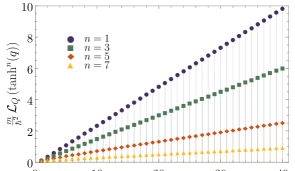
Figure 1: (Color Online) Bound $\mathcal{L}_{Q}(T_{0}(q))$ of the quantum potential associated to the eigenstates of the Pöschl-Teller potential for the function $T_{0}(q)=\tanh^{n}(q)$. The case $n=1$ corresponds to the mean value of the quantum potential, i.e., $\mathcal{L}_{Q}(\tanh(q))=\left\langle Q\right\rangle$.

Let us now consider the uncertainty relation (53) for a linear function $T_{0}(q)=\zeta q+\zeta_{0}$. In accordance with (53), we need to determine the position variance, which is given by a generalized hypergeometric function ${}_{r}{\rm F}_{s}[(a_{r});(b_{s});z]$ Gradshteyn and Ryzhik (2007). Indeed, we have

$$\begin{split}\Delta q^{2}&=\int^{+\infty}_{-\infty}\!\!\!\![{\psi}_{\mu}^{\mu}(q)]^{2}q^{2}dq=\frac{(2\mu-1)!!}{(2\mu-2)!!}\int^{\infty}_{0}\!\!\!\!\!{\rm sech}^{2\mu}(q)\,q^{2}dq\\ &=\frac{2^{\mu-1}(2\mu-1)!!}{\mu^{2}\,\mu!}\,_{4}{\rm F}_{3}\!\left[\begin{array}[]{c}\mu\hskip 11.38092pt\mu\hskip 11.38092pt\mu\hskip 11.38092pt2\mu\\ \mu+1\;\mu+1\;\mu+1\end{array};-1\right]\ .\end{split}$$

In Fig.2, we compare the bound function with the MVQP (case $n=1$ in Fig.1). Note that the uncertainty relation for the linear function (53) gives a stronger constraint than the next function in Fig.1, i.e., the case $n=3$.

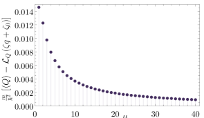
Figure 2: (Color Online) Difference between the mean value of the quantum potential and the bound $\mathcal{L}_{Q}(\zeta q+\zeta_{0})$ for the eigenstates of the Pöschl-Teller potential. The mean value $\left\langle Q\right\rangle$ is the curve $n=1$ in Fig.1.

As a final remark, note that the wave function for $\lambda=\mu$ corresponds to the most excited states. As $\mu$ increases, the behavior of the system approaches a plane wave and $Q(q,t)\to 0$ for $q\to\pm\infty$. Numerical tests up to $n\sim 10^{3}$ show that the monotonic decrease observed in Fig.2 is persistent. Thus the quantum potential approaches the linear bound function in this limit, even though the wave function of a free particle does not belong to the set $L^{2}(\Omega^{2})$, and the Cauchy-Schwartz inequality is not applicable.

VIII Conclusions and Final Comments

The debate on interpretation of quantum mechanics has been centered on the properties of the quantum potential and rarely makes any connection between the QP and the uncertainty relations. Instead of focusing on the quantum potential, in the present work we analyzed the properties and physical meaning of its mean value.

In sec. III, we showed that the MVQP satisfies an inequality for an arbitrary scalar function $T_{0}\in L^{2}\left(\Omega^{2}\right)$ and, by suitably choosing this function, the MVQP is always positive and bounded from below. Furthermore, we derived a generalized uncertainty relation that is stronger than the Robertson-Schrödinger inequality.

The physical meaning of the MVQP is that it is related to the nonclassical part of the momentum covariance matrix. Decomposing it as $\widetilde{\mathbf{V}}=\widetilde{\mathbf{V}}_{\!\text{c}}+\widetilde{\mathbf{V}}_{\!\text{nc}}$, where $\widetilde{\mathbf{V}}_{\!\text{c}}$ is exactly the momentum covariance matrix of the classical Hamilton-Jacobi formalism, i.e. $\widetilde{\mathbf{V}}_{\!\text{c}}={\mathbf{Cov}}\!\left(\partial_{q}S,\partial_{q}S\right)$, the nonclassical part identifies with the MVQP, namely, $\widetilde{\mathbf{V}}_{\!\text{nc}}:=\left\langle-\frac{\hbar^{2}}{\Omega}\partial^{2}_{qq}\Omega\right\rangle$. Thus, the bound on MVQP implies that any quantum system has a minimum of quantum momentum correlation. While classical systems can have zero momenta correlations, quantum systems are always correlated.

The results obtained primarily for pure states are then generalized for density matrices describing mixed states. Using a spectral decomposition $\hat{\rho}=\sum_{k}\omega_{k}|\psi_{k}\rangle\!\langle\psi_{k}|$, where $|\psi_{k}\rangle$ are eigenstates, neither $\widetilde{\mathbf{V}}_{\!\text{c}}$ nor $\widetilde{\mathbf{V}}_{\!\text{nc}}$ can be decomposed exclusively as a convex combination of $\widetilde{\mathbf{V}}_{\!\text{c}}^{(k)}$ nor $\widetilde{\mathbf{V}}_{\!\text{nc}}^{(k)}$, respectively. Notwithstanding, $\widetilde{\mathbf{V}}_{\!\text{nc}}$ can still be written as a convex sum, namely, $\widetilde{\mathbf{V}}_{\!\text{nc}}=\sum_{k}\omega_{k}\widetilde{\mathbf{V}}_{\!\text{nc}}^{(k)}+\delta\widetilde{\mathbf{V}}_{\!\text{nc}}$ where the latter term is a symmetric positive-semidefinite matrix. As a consequence, the MVQP defined in (37) for mixed states is always greater than or equal to the sum of the MVQP for each pure state in the spectral decomposition. As a corollary, the MVQP for mixed states also has a positive lower bound.

The identification of the MVQP with the nonclassical part of the momentum covariance matrix allow us to interpret the semiclassical limit in an adequate manner, which might give new insights for this regime. Indeed, in reference Maia et al. (2008), the WBK propagation becomes a good description for the dynamics of the system when a dynamical stretching of the initial (non-WKB) Gaussian state along an unstable manifold of the classical dynamics is performed. On the lines developed here, this stretching is responsible for the vanishing of the quantum correlations. Thus, our studies might open up new connections in the influence of the quantum potential on the semiclassical propagation.

Appendices

Appendix A Pure Gaussian States

In this appendix we summarize some information about pure Gaussian states of a system with $n$ degrees of freedom and their symplectic evolution.

It is well known that a quadratic Hamiltonian generates a symplectic evolution and that this preserves the Gaussian character of an initial Gaussian state Littlejohn (1986). The most generic quadratic Hamiltonian can be constructed from the Hamiltonian in (3) with

$$U(q)=\tfrac{1}{2}q\cdot{\bf L}q+\xi_{q}\cdot q+H_{0}$$ (67)

where ${\bf L}={\bf L}^{\top}$ is a $n\times n$ symmetric real matrix, $\xi_{q}\in\mathbb{R}^{n}$ is a column vector, and $H_{0}$ is a real constant. Such a Hamiltonian is the generator of the uniparametric symplectic subgroup constituted by $\mathsf{S}_{t}$ such that

$${\mathsf{S}_{t}}:={\rm e}^{\mathsf{J}{\bf H}t},\,\,\,{\mathsf{J}}:=\left(\!\begin{array}[]{cc}0_{n}&\mathsf{I}_{n}\\ -\mathsf{I}_{n}&0_{n}\end{array}\!\right),\,\,\,{\bf H}:=\left(\!\begin{array}[]{lc}{\bf L}&{\bf C}\\ {\bf C}^{\top}&{\bf M}\end{array}\!\right).$$ (68)

A $2n\times 2n$ real matrix $\mathsf{S}$ is said to be symplectic if $\mathsf{S}\!^{\top}\!\!\mathsf{J}\mathsf{S}=\mathsf{S}\mathsf{J}\mathsf{S}\!^{\top}=\mathsf{J}$, which is the case of $\mathsf{S}_{t}$ in (68). These matrices can be partitioned into $n\times n$ blocks ${\bf a},{\bf b},{\bf c},{\bf d}$, as follows

$$\mathsf{S}=\!\left(\!\begin{array}[]{cc}\mathbf{a}&\mathbf{b}\\ \mathbf{c}&\mathbf{d}\end{array}\!\right)\!\,{\rm with}\left\{\!\!\begin{array}[]{ll}\mathbf{ad\!^{\top}}-\mathbf{bc\!^{\top}}=\mathsf{I}_{n},&\!\!\mathbf{a\!^{\top}\!c=c\!^{\top}\!a},\\ \mathbf{a\!^{\top}\!d}-\mathbf{c\!^{\top}\!b}=\mathsf{I}_{n},&\!\!\mathbf{ab\!^{\top}=ba\!^{\top}},\\ \mathbf{cd\!^{\top}=dc\!^{\top}},&\!\!\mathbf{b\!^{\top}\!d=d\!^{\top}\!b}.\end{array}\right.$$ (69)

The constraints over the blocks came from the symplectic nature of $\mathsf{S}$ Littlejohn (1986).

The wave function of a generic pure Gaussian state of $n$ DF always has the following structure Littlejohn (1986):

$$\psi(q,t)=\frac{{\rm e}^{-\frac{1}{2\hbar}(q-\eta_{q})\cdot{\bf\Sigma}_{\mathsf{S}}(q-\eta_{q})+\frac{i}{\hbar}(\eta_{p}\cdot q-\frac{1}{2}\eta_{q}\cdot\eta_{p})}}{{(\pi\hbar)^{\frac{n}{4}}\sqrt{\det{(\mathbf{a}+i\mathbf{b})}}}},$$ (70)

where

$${\bf\Sigma}_{\mathsf{S}}:=[\mathsf{I}_{n}-i(\bf{ca\!^{\top}}+\bf{db\!^{\top}})]({\bf aa\!^{\top}}+{\bf bb\!^{\top}})^{-1}$$ (71)

is a $n\times n$ matrix constructed with the $n\times n$ blocks of $\mathsf{S}$ in (69), $\eta_{q}:=\langle\psi|\hat{q}|\psi\rangle\in\mathbb{R}^{n}$ and $\eta_{p}:=\langle\psi|\hat{p}|\psi\rangle\in\mathbb{R}^{n}$ are, respectively, the mean value column vectors of position and momentum operators, see below.

Under the quadratic Hamiltonian, which generates $\mathsf{S}_{t}$ in (68), the state in (70) evolves into another Gaussian pure state with the same structure, but with the replacements Littlejohn (1986):

$${\bf\Sigma}_{\mathsf{S}}\rightarrow{\bf\Sigma}_{\mathsf{S}_{t}\mathsf{S}},\,\left(\!\begin{array}[]{c}\eta_{q}\\ \eta_{p}\end{array}\!\right)\rightarrow\mathsf{S}_{t}\left(\!\begin{array}[]{c}\eta_{q}\\ \eta_{p}\end{array}\!\right)+\int_{0}^{t}\!\!\!dt^{\prime}{\mathsf{S}}_{t^{\prime}}\mathsf{J}\!\left(\!\begin{array}[]{c}\xi_{q}\\ \xi_{p}\end{array}\!\right).$$ (72)

Since the product $\mathsf{S}_{t}\mathsf{S}$ is a member of the symplectic group, the generic structure in (70) is preserved by this temporal evolution.

The polar structure in (5) is readily obtained for the wave function in (70):

$$\begin{split}\Omega(q,t)&=\frac{\exp\left[-\frac{1}{4}(q-\eta_{q})\cdot{\bf V}^{-1}(q-\eta_{q})\right]}{\left[(2\pi)^{n}\det{\bf V}\right]^{1/4}},\\ S(q,t)&=\tfrac{1}{2}(q-\eta_{q})\cdot{\rm Im}({\bf\Sigma}_{\sf S})(q-\eta_{q})\\ &+(\eta_{p}\cdot q-\tfrac{1}{2}\eta_{q}\cdot\eta_{p})-\tfrac{\hbar}{2}\,{\rm Arg}[\det({\bf a}+i{\bf b})].\end{split}$$ (73)

In these last equations, the matrix $\bf V$ is the position covariance matrix in (29) and, for the Gaussian state in (70), is equal to

$${\bf V}=\frac{\hbar}{2}\left[{\rm Re}({\bf\Sigma}_{\sf S})\right]^{-1}=\frac{\hbar}{2}({\bf aa\!^{\top}}+{\bf bb\!^{\top}}),$$ (74)

and is determined by (71). Furthermore, the already defined mean values are written as

$$\begin{split}\eta_{q}&=\langle\psi|\hat{q}|\psi\rangle=\int_{\mathbb{R}^{n}}\!\!\!\!\!{\rm d}^{n}\!q\,\,[\Omega(q,t)]^{2}\,q.\\ \eta_{p}&=\langle\psi|\hat{p}|\psi\rangle=\int_{\mathbb{R}^{n}}\!\!\!\!\!{\rm d}^{n}\!q\,\,[\Omega(q,t)]^{2}\,\partial_{q}S(q,t).\end{split}$$

The mean value of the momenta vector is also in accordance with (32), i.e., $p_{\text{c}}=\eta_{p}$ for a Gaussian state.

Appendix B Convex Decomposition of $\widetilde{\mathbf{V}}_{\!\text{nc}}$

In this Appendix the reader will find the demonstration that the classical/quantum correlations of a mixed states can be written as a convex sum. In summary, we will show the relation among the matrix $\widetilde{\mathbf{V}}_{\!\text{nc}}$ in Eqs.(38) and the matrices $\widetilde{\mathbf{V}}_{\!\text{nc}}^{(k)}$ in Eq.(42). To this end we will only properly rewrite all the derivatives appearing in (38).

For a question of compactness, let us define $\rho_{qq^{\prime}}:=\langle q|\hat{\rho}|{q^{\prime}}\rangle$ for the matrix element in (11), and by the hermiticity of $\hat{\rho}$, it is clear that $\rho_{q^{\prime}\!q}=\rho_{qq^{\prime}}^{\ast}$. Using the spectral decomposition (41), we calculate

$$\begin{split}&\rho_{qq}=\bar{\Omega}(q,q,t)=\sum_{k}\omega_{k}|\psi_{k}^{\ast}(q)|^{2}=\sum_{k}\omega_{k}\,\Omega_{k}^{2},\\ &\partial_{j}\rho_{qq^{\prime}}|_{q^{\prime}=q}=\sum_{k}\omega_{k}\,\psi_{k}^{\ast}(q)\,\partial_{j}\psi_{k}(q)\\ &\hskip 45.52458pt=\sum_{k}\omega_{k}\left[\Omega_{k}\partial_{j}\Omega_{k}+\frac{i}{\hbar}\Omega_{k}^{2}\partial_{j}S_{k}\right],\\ \end{split}$$ (75)

with $\Omega_{k}=\Omega_{k}(q,t)$ being the amplitude and $S_{k}=S_{k}(q,t)$ the phase of $\psi_{k}(q)=\langle q|\psi_{k}\rangle$.

The amplitude in (11) can be written as

$$\bar{\Omega}(q,{q^{\prime}},t)=|\rho_{qq^{\prime}}|=\sqrt{\rho_{qq^{\prime}}\rho_{q^{\prime}\!q}}.$$

Taking the derivative with respect to $q_{j}$ and using (75), one has

$$\begin{split}\partial_{j}\bar{\Omega}|_{q^{\prime}=q}&=\left[\frac{1}{2\bar{\Omega}}\left(\rho_{q^{\prime}\!q}\partial_{j}\rho_{qq^{\prime}}+\rho_{qq^{\prime}}\partial_{j}\rho_{q^{\prime}\!q}\right)\right]_{q^{\prime}=q}\\ &=\tfrac{1}{2}\left[\partial_{j}\rho_{qq^{\prime}}+\partial_{j}\rho_{q^{\prime}\!q}\right]_{q^{\prime}=q}\\ &=\tfrac{1}{2}\sum_{k}\omega_{k}\,\partial_{j}|\psi_{k}(q)|^{2}=\tfrac{1}{2}\partial_{j}\bar{\Omega}(q,q,t).\end{split}$$ (76)

Note the factor $1/2$ at the end, which shows the noncommutation of the derivative with the selection of the diagonal term $q^{\prime}=q$.

A clever way to obtain the derivative of the phase of (11) is to write it as follows

$$\begin{split}\partial_{j}\bar{S}|_{q^{\prime}=q}&=-i\hbar\,\left[{\rm e}^{-\frac{i}{\hbar}\bar{S}(q,q^{\prime},t)}\,\partial_{j}{\rm e}^{\frac{i}{\hbar}\bar{S}(q,q^{\prime},t)}\right]_{q^{\prime}=q}\\ &=-i\hbar\,{\rm e}^{-\frac{i}{\hbar}\bar{S}(q,q,t)}\,\partial_{j}\!\!\left.\left(\frac{\rho_{qq^{\prime}}}{\bar{\Omega}}\right)\right|_{q^{\prime}=q}\\ &=\frac{1}{\bar{\Omega}(q,q,t)}\sum_{k}\omega_{k}\,\Omega_{k}^{2}\,\partial_{j}S_{k},\end{split}$$ (77)

where we used Eqs.(11), Eq.(75) and that $\bar{S}(q,q^{\prime}=q,t)=0$. Note that

$$\left\langle\partial_{j}\bar{S}|_{q^{\prime}=q}\right\rangle_{\rho}=\int_{\mathbb{R}^{n}}\!\!\!\!\!{\rm d}^{n}\!q\,\,\bar{\Omega}(q,q,t)\,\partial_{j}\bar{S}|_{q^{\prime}=q}=\sum_{k}\omega_{k}\,\left\langle\partial_{j}S_{k}\right\rangle$$

is the $j^{\text{th}}$ component of the classical momenta in (39).

Now, we calculate the second derivative of the amplitude and write it as

$$\partial^{2}_{ij}\bar{\Omega}|_{q^{\prime}=q}=\Phi_{1}(q,t)+\Phi_{2}(q,t)+\Phi_{3}(q,t).$$ (78)

The first term in the above equation is

$$\begin{split}\Phi_{1}(q,t):=&-\left[\frac{\partial_{i}\bar{\Omega}}{2\bar{\Omega}^{2}}\left(\rho_{q^{\prime}\!q}\,\partial_{j}\rho_{qq^{\prime}}+\rho_{qq^{\prime}}\,\partial_{j}\rho_{q^{\prime}\!q}\right)\right]_{q^{\prime}=q}\\ =&-\frac{1}{4\bar{\Omega}(q,q,t)}\partial_{i}\bar{\Omega}(q,q,t)\,\partial_{j}\bar{\Omega}(q,q,t),\end{split}$$

where we used (76) and the derivatives of $\rho_{qq^{\prime}}$ were calculated using (11). The second term is

$$\begin{split}\Phi_{2}(q,t):=&\left[\frac{1}{2\bar{\Omega}}\left(\rho_{q^{\prime}\!q}\,\partial^{2}_{ij}\rho_{qq^{\prime}}+\rho_{qq^{\prime}}\,\partial^{2}_{ji}\rho_{q^{\prime}\!q}\right)\right]_{q^{\prime}=q}\\ =&\sum_{k}\omega_{k}\,{\rm Re}\!\left[\psi_{k}^{\ast}(q)\,\partial^{2}_{ij}\psi_{k}(q)\right]\\ =&\sum_{k}\omega_{k}\Omega_{k}\partial^{2}_{ij}\Omega_{k}-\frac{1}{\hbar^{2}}\sum_{k}\omega_{k}\Omega_{k}^{2}\,\partial_{i}S_{k}\,\partial_{j}S_{k},\\ \end{split}$$

where we use Eq.(76) and the second derivatives were performed directly from Eq.(41). The last term is

$$\begin{split}\Phi_{3}(q,t):=&\left[\frac{1}{2\bar{\Omega}}\left(\partial_{i}\rho_{qq^{\prime}}\,\partial_{j}\rho_{q^{\prime}\!q}+\partial_{i}\rho_{q^{\prime}\!q}\,\partial_{j}\rho_{qq^{\prime}}\right)\right]_{q^{\prime}=q}\\ =&-\Phi_{1}(q,t)+\frac{1}{\hbar^{2}}\bar{\Omega}(q,q,t)\,\partial_{i}\bar{S}|_{q^{\prime}=q}\,\partial_{j}\bar{S}|_{q^{\prime}=q},\end{split}$$

where the derivatives were calculated using (11). Finally, comparing $\widetilde{\mathbf{V}}_{\!\text{nc}}$ in (38) with (78), we obtain the desired result:

$$\!\widetilde{\mathbf{V}}_{\!\text{nc}}=-\hbar^{2}\!\sum_{m=1}^{3}\!\int_{\mathbb{R}^{n}}\!\!\!{\rm d}^{n}\!q\,\,\Phi_{m}(q,t)=\!\sum_{k}\omega_{k}\widetilde{\mathbf{V}}_{\!\text{nc}}^{(k)}+\,\delta\widetilde{\bf V}_{\!\text{nc}},$$

where $\Phi_{1}$ cancels with part of $\Phi_{3}$, while the first summation in the final form of $\Phi_{2}$ gives rise to the summation of the quantum potentials in (42). The remaining terms of $\Phi_{2}$ and $\Phi_{3}$ are grouped in

$$\begin{split}\delta\widetilde{\bf V}_{\!\text{n}c}:=&\sum_{k}\omega_{k}\!\int_{\mathbb{R}^{n}}\!\!\!\!\!{\rm d}^{n}\!q\,\Omega_{k}^{2}\,\partial_{q}S_{k}(\partial_{q}S_{k})^{\!\top}-\int_{\mathbb{R}^{n}}\!\!\!\!\!{\rm d}^{n}\!q\,\bar{\Omega}(q,q,t)\,\partial_{q}\bar{S}|_{q^{\prime}=q}\,(\partial_{q}\bar{S}|_{q^{\prime}=q})^{\top}\\ =&\sum_{k}\omega_{k}\!\int_{\mathbb{R}^{n}}\!\!\!\!\!{\rm d}^{n}\!q\,\Omega_{k}^{2}\left(\partial_{q}S_{k}-\partial_{q}\bar{S}|_{q^{\prime}=q}\right)\!\!\left(\partial_{q}S_{k}-\partial_{q}\bar{S}|_{q^{\prime}=q}\right)^{\!\!\top}.\end{split}$$ (79)

From its structure, the matrix $\delta{\bf V}_{\!\text{nc}}$ is a positive-semidefinite matrix, which is the most important observation of this appendix.

References

- Bohm (1952a) D. Bohm, Physical Review 85, 166 (1952a).
- Bohm (1952b) D. Bohm, Physical Review 85, 180 (1952b).
- Bohm and Hiley (1984) D. Bohm and B. J. Hiley, Foundations of Physics 14, 255 (1984).
- Bohm et al. (1987) D. Bohm, B. J. Hiley, and P. N. Kaloyerou, Physics Reports 144, 321 (1987).
- Holland (1993) P. R. Holland, The Quantum Theory of Motion: An Account of the de Broglie-Bohm Causal Interpretation of Quantum Mechanics (Cambridge University Press, 1993).
- Durr et al. (1995) D. Durr, S. Goldstein, and N. Zanghi, (1995), arXiv:quant-ph/9511016 [quant-ph] .
- Valentini (1991) A. Valentini, Phys. Lett. A156, 5 (1991).
- Valentini and Westman (2005) A. Valentini and H. Westman, Proceedings of the Royal Society A: Mathematical, Physical and Engineering Sciences 461, 253 (2005).
- Towler et al. (2012) M. D. Towler, N. J. Russell, and A. Valentini, Proceedings of the Royal Society A: Mathematical, Physical and Engineering Sciences 468, 990 (2012).
- Efthymiopoulos and Contopoulos (2006) C. Efthymiopoulos and G. Contopoulos, Journal of Physics A: Mathematical and General 39, 1819 (2006).
- Bennett (2010) A. F. Bennett, Journal of Physics A: Mathematical and Theoretical 43, 195304 (2010).
- Falciano et al. (2013) F. T. Falciano, N. Pinto-Neto, and S. D. P. Vitenti, Phys. Rev. D87, 103514 (2013), arXiv:1305.4664 [gr-qc] .
- Vitenti et al. (2013) S. D. P. Vitenti, F. T. Falciano, and N. Pinto-Neto, Phys. Rev. D87, 103503 (2013), arXiv:1206.4374 [gr-qc] .
- Vitenti et al. (2014) S. D. P. Vitenti, F. T. Falciano, and N. Pinto-Neto, Phys. Rev. D89, 103538 (2014), arXiv:1311.6730 [astro-ph.CO] .
- Pinto-Neto and Fabris (2013) N. Pinto-Neto and J. C. Fabris, Classical and Quantum Gravity 30, 143001 (2013), arXiv:1306.0820 [gr-qc] .
- Struyve (2015) W. Struyve, (2015), arXiv:1507.04771 [quant-ph] .
- Benseny et al. (2014) A. Benseny, G. Albareda, A. S. Sanz, J. Mompart, and X. Oriols, Eur. Phys. J. D68, 286 (2014), arXiv:1406.3151 [quant-ph] .
- Struyve (2019) W. Struyve, (2019), ArXiv:1902.02188 [gr-qc] .
- Carroll (2007) R. Carroll, (2007), arXiv:0705.3921 [gr-qc] .
- Carroll (2007) R. Carroll, On the Quantum potential (Abramis, United Kingdom, 2007).
- Novello et al. (2011) M. Novello, J. M. Salim, and F. T. Falciano, Int. J. Geom. Meth. Mod. Phys. 8, 87 (2011).
- Falciano et al. (2010) F. T. Falciano, M. Novello, and J. M. Salim, Found. Phys. 40, 1885 (2010).
- Frieden and Soffer (1995) B. R. Frieden and B. H. Soffer, Phys. Rev. E 52, 2274 (1995).
- Reginatto (1998) M. Reginatto, Phys. Rev. A 58, 1775 (1998).
- Frieden (1988) B. R. Frieden, Journal of Modern Optics 35, 1297 (1988).
- Frieden (1989) B. R. Frieden, American Journal of Physics 57, 1004 (1989).
- Frieden (1998) B. R. Frieden, Physics from Fisher Information: A Unification (Cambridge University Press, 1998).
- Hall (2000) M. J. W. Hall, Phys. Rev. A 62, 012107 (2000).
- Hall (2001) M. J. W. Hall, Phys. Rev. A 64, 052103 (2001).
- Hall and Reginatto (2002) M. J. W. Hall and M. Reginatto, J. Phys. A: Math. Gen 35, 3289 (2002).
- Kulkarni et al. (1999) D. Kulkarni, D. Schmidt, and S.-K. Tsui, Linear Algebra and its Applications 297, 63 (1999).
- Sakurai (1994) J. J. Sakurai, Modern quantum mechanics (Addison Wesley, 1994).
- Cohen-Tannoudji et al. (1977) C. Cohen-Tannoudji, B. Diu, and F. Laloe, Quantum Mechanics (John Wiley & Sons, 1977).
- Robertson (1929) H. P. Robertson, Phys. Rev. 34, 163 (1929).
- Schroedinger (1930) E. Schroedinger, Zum Heisenbergschen Unschaerfeprinzip, Sitzungsberichte der Preussischen Akademie der Wissenschaften, Physikalisch-mathematische Klasse 14, 296 (1930).
- Gelfand and Fomin (1963) I. M. Gelfand and S. V. Fomin, Calculus of Variations (Prentice-Hall, New-Jersey, 1963).
- Horn and Johnson (2013) R. A. Horn and C. R. Johnson, Matrix Analysis (Cambridge University Press, New York, 2013).
- Maia et al. (2008) R. N. P. Maia, F. Nicacio, R. O. Vallejos, and F. Toscano, Phys. Rev. Lett. 100, 184102 (2008).
- Cox and Hinkley (1974) D. R. Cox and D. V. Hinkley, Theoretical Statistics (Springer-Science+Business Media, B.V., London, 1974).
- Simon (2000) R. Simon, Phys. Rev. Lett. 84, 2726 (2000).
- Gradshteyn and Ryzhik (2007) I. S. Gradshteyn and I. M. Ryzhik, Table of Integrals, Series, and Products (Elsevier, Amsterdam, 2007).
- Anders and Winter (2008) J. Anders and A. Winter, Quantum Information & Computation 8, 245 (2008).
- Giorda and Paris (2010) P. Giorda and M. G. A. Paris, Phys. Rev. Lett. 105, 020503 (2010).
- Papoulis and Unnikrishna Pillai (2002) A. Papoulis and S. Unnikrishna Pillai, Probability, Random Variables and Stochastic Processes (McGraw-Hill, 2002).
- Pöschl and Teller (1933) G. Pöschl and E. Teller, Zeitschrift für Physik 83, 143 (1933).
- Littlejohn (1986) R. G. Littlejohn, Physics Reports 138, 193 (1986).