Locating ergostar models in parameter space
Abstract
Recently, we have shown that dynamically stable ergostar solutions (equilibrium neutron stars that contain an ergoregion) with a compressible and causal equation of state exist [A. Tsokaros, M. Ruiz, L. Sun, S. L. Shapiro, and K. Uryū, Phys. Rev. Lett. 123, 231103 (2019)]. These stars are hypermassive, differentially rotating, and highly compact. In this work, we make a systematic study of equilibrium models in order to locate the position of ergostars in parameter space. We adopt four equations of state that differ in the matching density of a maximally stiff core. By constructing a large number of models both with uniform and differential rotation of different degrees, we identify the parameters for which ergostars appear. We find that the most favorable conditions for the appearance of dynamically stable ergostars are a significant finite density close to the surface of the star (i.e., similar to self-bound quark stars) and a small degree of differential rotation.
I Introduction
One important open question in modern astrophysics is the mechanism that powers relativistic jets in short gamma-ray bursts like the one accompanying event GW170817 Abbott et al. (2017); Savchenko et al. (2017, ). Within the membrane paradigm, these highly energetic phenomena are typically attributed to the black hole horizon Thorne et al. (1986). On the other hand, according to more recent studies Komissarov (2004, 2005); Ruiz et al. (2012), it is the ergosphere and its threading by magnetic field lines that is chiefly responsible for the jet’s existence, while a black hole horizon is not necessary. An ergostar is a star that contains an ergoregion, i.e., a region where there are no timelike static observers and all trajectories (timelike or null) must rotate in the direction of rotation of the star (frame dragging). For an ergostar, the question relevant to jet formation is whether the ergoregion is preserved in the presence of a dissipative mechanism, such as viscosity or a turbulent magnetic field. In particular, when an ergostar is threaded by a magnetic field, is stability maintained over many Alfvén timescales, or does the turbulent magnetic viscosity destabilize the star before a jet can be launched?
The question regarding the dynamical stability of an ergostar with a causal and compressible equation of state (EOS) was answered positively in Tsokaros et al. (2019). There, the ALF2cc EOS was adopted to create ergostars that evolved stably for dynamical times or rotation periods. These equilibria, when perturbed in a radial or nonaxisymmetric way, showed no significant mode growth, while their shape and ergoregion remained intact. At the same time, polytropic models of ergostars presented in Komatsu et al. (1989) proved to be unstable to radial collapse. The secular evolution of stars containing ergoregions is governed by the fact that the timelike Killing vector associated with the stationarity of the spacetime becomes spacelike inside the ergoregion, which implies a negative energy with respect to an asymptotic observer for a freely moving particle there. As a consequence, a nonaxisymmetric perturbation that radiates positive energy at infinity will make the negative energy in the ergoregion even more negative, leading to the so-called Friedman instability Friedman (1978); Moschidis (2018). The timescale for this instability was initially considered to be longer than the Hubble time Comins and Schutz (1978), but more recently, it was found that it can be quite small Yoshida and Eriguchi (1996); Brito et al. (2015) (for small mode numbers).
On the other hand, since the original work of Wilson Wilson (1972), it seems that differential rotation plays a crucial role in the appearance of an ergoregion (see also the models of Butterworth and Ipser (1975); Komatsu et al. (1989); Ansorg et al. (2002)). In the presence of magnetic fields, this differential rotation is eventually suppressed due to magnetic winding and the magnetorotational instability Shapiro (2000); Duez et al. (2006), which in turn implies that jet formation (if dependent on the existence of the ergoregion) may be inhibited. Given the fact that we were able to construct dynamically stable, differentially rotating ergostars, the answer regarding the ergosphere hypothesis on jet formation depends crucially on whether a dissipative mechanism will affect the structure of the ergostar sufficiently to remove the ergoregion before powering a jet. Alternatively, they may drive an ergostar, if hypermassive, to collapse to a black hole. If the ergosphere is indeed responsible for the formation of a jet, then in this case, its lifetime may be different from the case where a black hole is the power source.
In order to probe the possible scenarios described above, one needs to know the most favorable equilibria that contain ergoregions. Is it possible to have ergostars that are uniformly rotating (with a compressible and causal EOS)? Is it possible to have supramassive Cook et al. (1992) ergostars, i.e., uniformly rotating ergostars with mass larger than the maximum Tolman-Oppenheimer-Volkoff (TOV) limit, but less than the maximum mass at the mass-shedding (Kepler) limit? To answer such questions, we perform in this work a parameter study probing the existence of ergostars. Using four EOSs and different degrees of differential rotation, we map the location of the ergostars on mass vs central density diagrams. Our EOS strategy is similar to the one employed in Tsokaros et al. (2019). This time, we start with the SLy EOS Douchin and Haensel (2001) and construct a large number of uniformly and differentially rotating models using 5 degrees of differential rotation. Then we construct three additional EOSs based on the SLy one where we progressively substitute an inner core at matching densities with the maximally stiff EOS, which has the speed of sound equal to the speed of light [see Eq. (4)]. Here, is nuclear matter density. Sequences of constant angular momentum and constant rest mass are constructed and stability questions are addressed.
II Numerical methods
Our equilibria are constructed with the Cook-Shapiro-Teukolsky (CST) code Cook et al. (1992), which solves the Einstein equations for rotating equilibria under the assumptions of stationarity and axisymmetry. The spacetime element (units of ) is in the form of
| (1) | |||||
where are all functions of and only, while the stress-energy tensor is written as
| (2) |
where is the rest-mass density, the internal energy density, and the pressure at the rest frame of the fluid. Here, is the fluid four-velocity that for a circular flow considered here may be written as , where is the timelike Killing vector that defines stationarity, and is the azimuthal spacelike Killing vector that defines axisymmetry. The angular velocity is constant for uniform rotation but a function of and when differential rotation is considered. The vanishing divergence of the stress-energy tensor, together with the assumptions of stationarity and axisymmetry, lead to the Euler equation of hydrostatic equilibrium Cook et al. (1992). In the case of uniform rotation, the Euler equation can be directly integrated, while in the case of differential rotation, it can be integrated when the specific angular momentum is a function of itself Cook et al. (1992); Uryū et al. (2016). In this work, we will consider either uniform rotation or differential rotation described by the Komatsu-Eriguchi-Hachisu law Komatsu et al. (1989, 1989) , where is the angular velocity at the center of the star, and is a parameter that controls the amount of differential rotation. To probe for the existence of the ergosphere, we examine at every point the sign of the norm of the vector , and in particular, we identify where the condition
| (3) |
is satisfied.
| - | |
|---|---|
The first EOS that we consider here uses the SLy EOS Douchin and Haensel (2001) in the form of a piecewise representation Read et al. (2009). The matching rest-mass densities as well as the polytropic indices are shown in Table 1. A polytropic constant is calculated from the reference values of pressure () and density (), while the rest of the polytropic constants are calculated from the equality of pressure at the dividing densities of Table 1. The other three EOSs (SLycc1, SLycc2, and SLycc4) are based on the SLy one where we progressively substitute an inner core at matching densities , and , with the maximally stiff EOS Haensel and Zdunik (1989)
| (4) |
Here, is a dimensionless parameter, is the total energy density, and the pressure at . The solutions presented in this work assume , i.e., a core at the causal limit, which represents the compressible EOS that yields configurations of maximal compactness Lattimer and Prakash (2016). Equation (4) relates the pressure to the total energy density when for the SLycc1, SLycc2, and SLycc4 EOSs respectively, while for the SLy EOS is recovered. One can express the pressure in terms of the rest-mass density in a polytropiclike form by integrating the first law of the thermodynamics . Using Eq. (4), we get for ,
| (5) | |||||
| (6) | |||||
| (7) |
where the constant , and is the specific enthalpy. The value can be evaluated from the polytrope outside the core.
| EOS | ||||
|---|---|---|---|---|
| SLy | ||||
| SLycc1 | ||||
| SLycc2 | ||||
| SLycc4 |
III Results
For the four EOSs described above the maximum spherical mass , the maximum mass at the mass-shedding limit under uniform rotation , as well as their corresponding rest-mass densities are shown in Table 2. We note here that the SLy EOS has a speed of sound larger than the speed of light when which is identical to the density at the maximum mass. For the other three EOSs, since is less than this value, we always have .
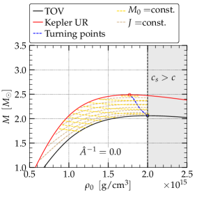

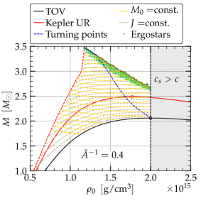
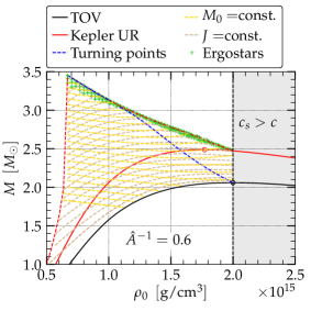

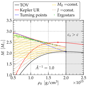
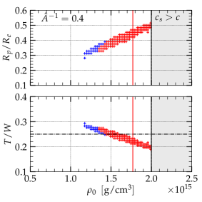
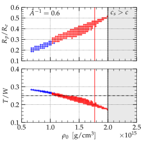

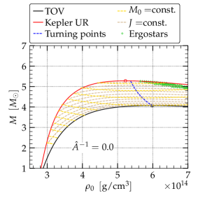

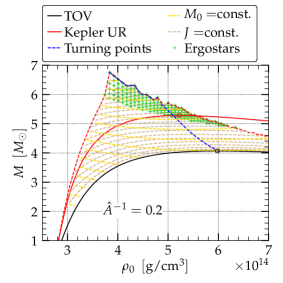
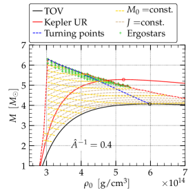
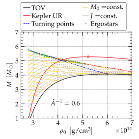
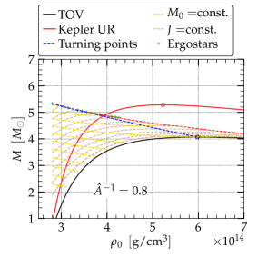
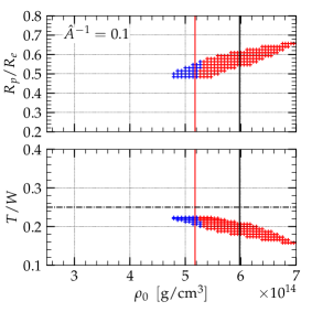
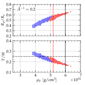
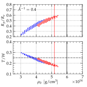
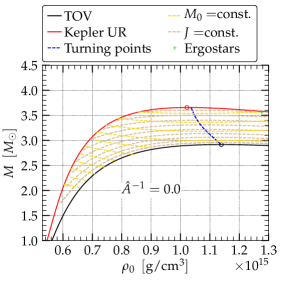
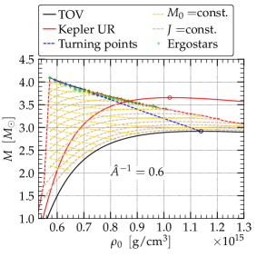
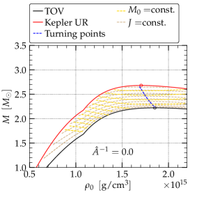
Figure 1 is devoted to the SLy EOS. The top and middle rows depict the position of ergostars (green crosses) in a mass vs central rest-mass density diagram.111Here we use the notation of the CST code Cook et al. (1992) where , being the equatorial radius. Every panel corresponds to a different degree of differential rotation starting from uniform rotation in the top left panel where and progressing to a higher degree of differential rotation in the right middle panel where . In each plot, we show the spherical solutions (TOV black curve), the mass-shedding limit of uniformly rotating stars (red curve), sequences of constant rest mass (orange dashed curves), sequences of constant angular momentum (brown dashed curves), and the curve that joins the maximum mass points (turning points) on every sequence (blue dashed curve). In a typical calculation, for every (i.e., for every panel) we divide a range of densities starting from a low density up to the limiting point into intervals, and using the CST code we compute constant rest-mass density sequences from the spherical limit (black curve) all the way up into more massive models that have small ratios until the code fails to converge. Here, is the polar radius. The last points, i.e., the points with the smaller value of , on every sequence are connected with a dashed red curve in the panels of the top and middle row in Fig. 1. As we can see, there are no ergostars for uniformly rotating models or small differential rotation for the SLy EOS. On the other hand, the largest number of ergostars appear when is approximately in the range , while for larger degrees of differential rotation, they tend to diminish again.
One important line in these plots is the blue dashed line which separates the secularly unstable/stable models against axisymmetric perturbations. For the uniformly rotating case, it is denoted as the turning point line due to “turning point theorem” of Friedman, et al. Friedman et al. (1988): Along a sequence of uniformly rotating stars with fixed angular momentum and increasing central density, the configuration of maximum mass marks the onset of secular instability. The turning point line is also commonly taken to be the criterion for distinguishing dynamical stability. Although the analysis of Takami et al. Takami et al. (2011) implies that the loci of secular, dynamical, and turning point lines is more subtle, they clearly are close to each other. For differential rotation, there is no analogous theorem, but there is significant evidence that again the locus of dynamical stability is very close to the turning point on const curves Kaplan et al. (2014); Bauswein and Stergioulas (2017); Weih et al. (2018). According to Takami et al. (2011); Weih et al. (2018), the dynamical instability typically sets in at central densities slightly below the one that corresponds to the turning point. In particular, as one moves along a const sequence toward increasing densities, one encounters the secular instability first, then the dynamical, and finally the turning point. Given that all three points are very close together and given the lack of any general theorem, we will assume here that the turning points mark the beginning of the dynamically unstable region, although the reader should be aware of the differences discussed above. We also note here that in the cases with differential rotation, the CST code can go to large deformations (i.e., small ratios of ) that correspond to toroidal configurations. On the other, hand in some cases, especially for large masses and smaller densities, we were not able to find a turning point. Typically, for those cases a fixed angular momentum sequence is a monotonically increasing function of mass as one moves to larger densities. For our present purposes, we tacitly assume that the last points in those sequences signify the dynamical instability limit, although in reality that limit should be on the left at higher densities.222It is possible that more fine-tuned codes like Stergioulas and Friedman (1995); Ansorg et al. (2009) can go beyond our calculated models and refine the position of the turning point in the very high mass differentially rotating regime.
This implies that all ergostars on and to the right of the blue dashed lines are dynamically unstable. For the SLy EOS, Fig. 1, this criterion rules out most of the ergostars, at least for a mild degree of differential rotation (). For larger differential rotation, the ergostars tend to accumulate close to the turning point line (or more precisely, close to the last model we were able to calculate), and given the discussion above, the dynamical stability of these models is questionable, as a full evolution will be needed for a diagnosis. We also note here that as differential rotation becomes larger, the turning point line becomes straighter and rotates counterclockwise with respect to the maximum spherical point. This also implies that all models on and to the right of the uniformly rotating turning point line are dynamically unstable irrespective of the degree of differential rotation. In addition, this is true for supramassive as well as hypermassive stars.
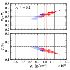
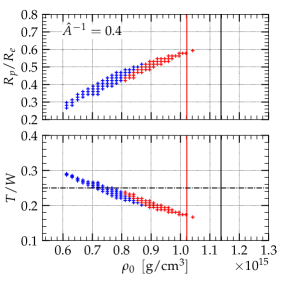
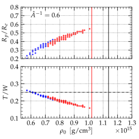
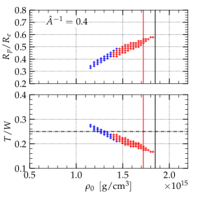
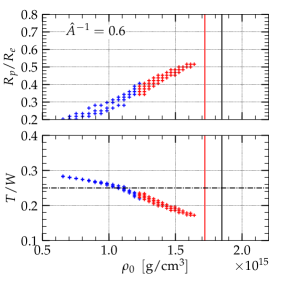
To get a better understanding of the qualitative features of the SLy ergostars, we plot in the bottom row of Fig. 1 the deformation parameter as well as the rotational kinetic over the gravitational potential energy for three representative cases of differential rotation. The vertical black line corresponds to the density of the maximum spherical mass, while the red one corresponds to the density of the maximum uniformly rotating mass. We find that all models with are toroidal (i.e., the maximum density is not at the center), and the larger the differential rotation, the more toroidal shapes we were able to compute. Note that according to recent studies Espino et al. (2019), extreme toroidal configurations are dynamically unstable. In the panels, we draw with a horizontal dashed-dot line the benchmark, which in many cases provides a crude criterion for the onset of dynamical instability to nonaxisymmetric (bar) modes Shibata et al. (2000); Baumgarte et al. (2000). Blue crosses correspond to ergostars on the left of the turning point line, while red crosses correspond to ergostars on the right of the turning point line.
Figure 2 is similar to Fig. 1, but it corresponds to the SLycc1 EOS. The effect of the large causal core is immediately seen even for the uniformly rotating models: Supramassive ergostars now appear, but they all lie in the dynamical unstable part of the parameter space. We also note here that the maximum mass of the spherical solutions, as well as the maximum mass at the mass-shedding limit, increase considerably from the SLy EOS (by factors of and , respectively). This has already been seen with the ALF2cc EOS employed in Tsokaros et al. (2019, 2020). Given the fact that the SLycc1 and ALF2cc EOSs only differ in the crust (i.e., for ), it is not surprising that the differences in the TOV and Kepler lines are minute. In addition, comparing SLycc1 vs SLy, we see that the densities where the maximum mass for the spherical and mass-shedding sequence reduce significantly (by factors of and , respectively; see Table 2). Although this may seem contradictory, it is related to the fact that the density profile along an axis is quite different from models using a typical EOS (like SLy or ALF2) without a large causal core. Instead of a parabolic type, the profile with SLycc1 starts from a smaller central density, diminishes somewhat all the way to the surface of the star, where it abruptly reduces to zero (see Fig. 1 in Tsokaros et al. (2020)). In this respect, stars with the SLycc1 or ALF2cc EOS resemble quark stars that have a finite surface density.
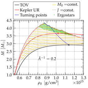

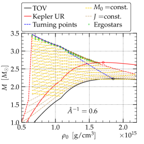

When differential rotation is considered, the general trends are (1) the turning point line moves up and turns counterclockwise with respect to the maximum TOV mass point, as in Fig. 1. (2) The ergostars move toward smaller densities well beyond the turning point line, toward the stable part of the parameter space. (3) For a larger degree of differential rotation, the ergostars tend to accumulate toward the turning point line and also the number of them tends to decrease. When differential rotation is large enough, the ergostars almost disappear.
The fact that a very mild differential rotation moved the ergostars from the unstable regime at high densities on the right of the turning point line to the left at lower central densities enabled us to find dynamically stable models Tsokaros et al. (2019). Although these models used a different EOS (ALF2cc), they do not differ significantly from the models of Fig. 2 since apart from a small crust, the rest of the star has the same (causal) EOS. In particular, the featured model in Fig. 1 of Tsokaros et al. (2019) had , a central density , and mass . Looking at the right panel of the top row in Fig. 2, we can see that indeed such a model lies within the dynamically stable regime.
From the bottom row panels of Fig. 2, where differential rotation is small () all ergostars are spheroidal for the SLycc1 EOS, and they progressively become toroidal with higher differential rotation (this is in contrast with the SLy EOS where almost all ergostars found had toroidal topology). Also, for the spheroidal models is below the benchmark value of , while it becomes larger and reaches the value as differential rotation is increased. We note here that for , the ergostars to the right of the blue line (which are the majority of them) should be unstable to axisymmetric perturbations. For the small number of ergostars to the left of the red line the possibility of dynamical stability is significant. For , all models with density larger than approximately should also be unstable to axisymmetric perturbations, but the ones with less central density can be stable even with respect to nonaxisymmetric modes (there are many models with and even some with can be stable). Similar arguments can be made for .
When the causal core is assumed at , ergostars almost disappear from the uniformly rotating regime (Fig. 3 top left panel). Similar to the SLycc1 EOS, small differential rotation () brings ergostars into the stable side of the turning point line and, according to Fig. 3 second row left panel, these are possibly stable against nonaxisymmetric perturbations. As the degree of differential rotation increases, the turning point line turns counterclockwise with respect to the maximum spherical mass point, and the ergostars accumulate toward the end point of our convergence regime. The middle and right panels in the second row of Fig. 3 show the deformation and when for the SLycc2 EOS. Full simulations will be needed to probe the fate of these equilibria. The bottom two rows in Fig. 3 depict the ergostars when the causal core shifts at . Here, the EOS is very close to the original SLy, apart from the very high density regime; thus, the position of the ergostars resembles the one found in Fig. 1.
IV Discussion
It has recently been proposed Komissarov (2004, 2005) that the mechanism behind the launching of relativistic jets from compact objects is the ergosphere and not a black hole horizon. In Ruiz et al. (2012), the authors tested a simplified version of this scenario by performing a force-free numerical simulation of a homogeneous ergostar using the Cowling approximation. They confirmed that the Blandford-Znajek mechanism is not directly related to the horizon of the black hole by showing that (a) the magnetic field collimation, (b) the induced charged density and poloidal currents, and (c) the electromagnetic luminosity that are produced by a rotating ergostar are similar to those observed in a rotating black hole spacetime. Their use of an incompressible EOS together with their freezing of the gravitational field, raises doubts regarding the stability of ergostars in a realistic evolutionary scenario. As in Ruiz et al. (2018, 2016); Paschalidis et al. (2015), we define an incipient jet based on the following three characteristics: (1) a collimated, tightly wound magnetic field, (2) a mildly relativistic outflow (), and (3) the outflow is confined by a funnel containing a (nearly) force-free magnetic field . Here, , and is the magnetic field at the poles. In the case of Ruiz et al. (2012), the absence of all matter does not permit conditions (2) and (3) to be checked, which motivates our efforts to explore the parameter space of dynamically stable ergostars with a compressible and causal EOS.
Regarding the Friedman instability, it was shown that the bar mode of a homogeneous ergostar having a period has a growth time Yoshida and Eriguchi (1996). Larger values of have even larger . On the other hand, the Alfvén timescale is
| (8) |
For typical ergostars and , one gets . Therefore, it is improbable that the Friedman instability will have any effect on the possible formation of a jet. On the other hand, large magnetic fields () are needed to bring the Alfvén timescale on levels that can be currently simulated () but sufficiently small that they are not dynamically significant initially.
In this work, we constructed more than uniformly and differentially rotating equilibria using four EOSs in order to probe the parameter space and identify the parameters under which ergostars appear. The most favorable parameters will be adopted in the future for full magnetohydrodynamical simulations. Using the SLy EOS as a basis, we constructed three other EOSs by imposing a causal core at , and . We expect that similar behavior will be found when any other EOS is used instead of the SLy one. The differential rotation law that we explored is the so-called “-const” law, and it will be interesting in the future to see how robust our findings are when other differential rotating laws are employed, like those presented in Uryū et al. (2017) that model more accurately the rotation profile of a neutron star merger remnant. In all cases considered, we calculated the turning point line Friedman et al. (1988) and commented on the stability properties of the ergostars that we found. For a regular EOS like the SLy, most ergostars appear on the unstable side of the turning point line, but for small differential rotation, models on the stable side also appear. These stars typically are highly hypermassive and very close to the limits of convergence for the CST code. Their stability will have to be probed by full general relativistic simulations as in Tsokaros et al. (2019). For an EOS like SLycc1, ergostars appear more frequently for a mild degree of differential rotation. Here, dynamically stable models exist, as shown in Tsokaros et al. (2019). Given the fact that the stars of this EOS resemble quark stars, we conjecture that stable ergostars of quark or strange matter will have more favorable possibilities for existence. When a causal core is found deep in the high density regime of a neutron star, the number of ergostars that we were able to construct diminished.
V Acknowledgments.
This work was supported by National Science Foundation Grant No. PHY-1662211 and the National Aeronautics and Space Administration (NASA) Grant No. 80NSSC17K0070 to the University of Illinois at Urbana-Champaign. This work made use of the Extreme Science and Engineering Discovery Environment, which is supported by National Science Foundation Grant No. TG-MCA99S008. This research is part of the Blue Waters sustained-petascale computing project, which is supported by the National Science Foundation (Grants No. OCI-0725070 and No. ACI-1238993) and the State of Illinois. Blue Waters is a joint effort of the University of Illinois at Urbana-Champaign and its National Center for Supercomputing Applications. Resources supporting this work were also provided by the NASA High-End Computing Program through the NASA Advanced Supercomputing Division at Ames Research Center.
References
- Abbott et al. (2017) B. P. Abbott et al. (Virgo, LIGO Scientific), Phys. Rev. Lett. 119, 161101 (2017), arXiv:1710.05832 [gr-qc] .
- Savchenko et al. (2017) V. Savchenko et al., Astrophys. J. 848, L15 (2017), arXiv:1710.05449 [astro-ph.HE] .
- (3) V. Savchenko et al., GCN Circular No. 21507, 2017 .
- Thorne et al. (1986) K. S. Thorne, R. H. Price, and D. A. Macdonald, The Membrane Paradigm (Yale University Press, New Haven, 1986).
- Komissarov (2004) S. S. Komissarov, Mon. Not. Roy. Astron. Soc. 350, 407 (2004), arXiv:astro-ph/0402403 .
- Komissarov (2005) S. S. Komissarov, Mon. Not. Roy. Astron. Soc. 359, 801 (2005), arXiv:astro-ph/0501599 .
- Ruiz et al. (2012) M. Ruiz, C. Palenzuela, F. Galeazzi, and C. Bona, Mon.Not.Roy.Astron.Soc. 423, 1300 (2012).
- Tsokaros et al. (2019) A. Tsokaros, M. Ruiz, L. Sun, S. L. Shapiro, and K. Uryū, Phys. Rev. Lett. 123, 231103 (2019), arXiv:1907.03765 [gr-qc] .
- Komatsu et al. (1989) H. Komatsu, Y. Eriguchi, and I. Hachisu, Monthly Notices of the Royal Astronomical Society 239, 153 (1989).
- Friedman (1978) J. L. Friedman, Communications in Mathematical Physics 63, 243 (1978).
- Moschidis (2018) G. Moschidis, Communications in Mathematical Physics 358, 437 (2018), arXiv:1608.02035 [math.AP] .
- Comins and Schutz (1978) N. Comins and B. Schutz, Proceedings Of The Royal Society Of London A Mathematical And Physical Sciences 364, 211 (1978).
- Yoshida and Eriguchi (1996) S. Yoshida and Y. Eriguchi, Monthly Notices of the Royal Astronomical Society 282, 580 (1996).
- Brito et al. (2015) R. Brito, V. Cardoso, and P. Pani, Lect. Notes Phys. 906, pp.1 (2015), arXiv:1501.06570 [gr-qc] .
- Wilson (1972) J. R. Wilson, Astrophys. J. 176, 195 (1972).
- Butterworth and Ipser (1975) E. M. Butterworth and J. R. Ipser, Astrophys. J. 200, L103 (1975).
- Ansorg et al. (2002) M. Ansorg, A. Kleinwachter, and R. Meinel, Astron. Astrophys. 381, L49 (2002), arXiv:astro-ph/0111080 [astro-ph] .
- Shapiro (2000) S. L. Shapiro, Astrophys.J. 544, 397 (2000).
- Duez et al. (2006) M. D. Duez, Y. T. Liu, S. L. Shapiro, M. Shibata, and B. C. Stephens, Physical Review Letters 96, 031101 (2006).
- Cook et al. (1992) G. B. Cook, S. L. Shapiro, and S. A. Teukolsky, Astrophys. J. 398, 203 (1992).
- Douchin and Haensel (2001) F. Douchin and P. Haensel, Astron. Astrophys. 380, 151 (2001), arXiv:astro-ph/0111092 .
- Uryū et al. (2016) K. Uryū, A. Tsokaros, F. Galeazzi, H. Hotta, M. Sugimura, K. Taniguchi, and S. Yoshida, Phys. Rev. D93, 044056 (2016).
- Komatsu et al. (1989) H. Komatsu, Y. Eriguchi, and I. Hachisu, Mon. Not. Roy. Astron. Soc. 237, 355 (1989).
- Read et al. (2009) J. S. Read, B. D. Lackey, B. J. Owen, and J. L. Friedman, Phys. Rev. D79, 124032 (2009).
- Haensel and Zdunik (1989) P. Haensel and J. L. Zdunik, Nature (London) 340, 617 (1989).
- Lattimer and Prakash (2016) J. M. Lattimer and M. Prakash, Phys. Rept. 621, 127 (2016).
- Friedman et al. (1988) J. L. Friedman, J. R. Ipser, and R. D. Sorkin, Astrophys. J. 325, 722 (1988).
- Takami et al. (2011) K. Takami, L. Rezzolla, and S. Yoshida, Mon. Not. Roy. Astron. Soc. 416, L1 (2011), arXiv:1105.3069 [gr-qc] .
- Kaplan et al. (2014) J. D. Kaplan, C. D. Ott, E. P. O’Connor, K. Kiuchi, L. Roberts, and M. Duez, Astrophys. J. 790, 19 (2014), arXiv:1306.4034 [astro-ph.HE] .
- Bauswein and Stergioulas (2017) A. Bauswein and N. Stergioulas, Mon. Not. Roy. Astron. Soc. 471, 4956 (2017), arXiv:1702.02567 [astro-ph.HE] .
- Weih et al. (2018) L. R. Weih, E. R. Most, and L. Rezzolla, Mon. Not. Roy. Astron. Soc. 473, L126 (2018), arXiv:1709.06058 [gr-qc] .
- Stergioulas and Friedman (1995) N. Stergioulas and J. Friedman, Astrophys. J. 444, 306 (1995), arXiv:astro-ph/9411032 [astro-ph] .
- Ansorg et al. (2009) M. Ansorg, D. Gondek-Rosińska, and L. Villain, Monthly Notices of the Royal Astronomical Society 396, 2359–2366 (2009).
- Espino et al. (2019) P. L. Espino, V. Paschalidis, T. W. Baumgarte, and S. L. Shapiro, Phys. Rev. D100, 043014 (2019), arXiv:1906.08786 [astro-ph.HE] .
- Shibata et al. (2000) M. Shibata, T. W. Baumgarte, and S. L. Shapiro, The Astrophysical Journal 542, 453 (2000).
- Baumgarte et al. (2000) T. W. Baumgarte, S. L. Shapiro, and M. Shibata, Astrophys. J. 528, L29 (2000), arXiv:astro-ph/9910565 [astro-ph] .
- Tsokaros et al. (2020) A. Tsokaros, M. Ruiz, S. L. Shapiro, L. Sun, and K. Uryū, Phys. Rev. Lett. 124, 071101 (2020), arXiv:1911.06865 [astro-ph.HE] .
- Ruiz et al. (2018) M. Ruiz, S. L. Shapiro, and A. Tsokaros, Phys. Rev. D98, 123017 (2018), arXiv:1810.08618 [astro-ph.HE] .
- Ruiz et al. (2016) M. Ruiz, R. N. Lang, V. Paschalidis, and S. L. Shapiro, Astrophys. J. 824, L6 (2016).
- Paschalidis et al. (2015) V. Paschalidis, M. Ruiz, and S. L. Shapiro, Astrophys. J. Letters 806, L14 (2015).
- Uryū et al. (2017) K. Uryū, A. Tsokaros, L. Baiotti, F. Galeazzi, K. Taniguchi, and S. Yoshida, Phys. Rev. D96, 103011 (2017), arXiv:1709.02643 [astro-ph.HE] .