All-In-One Robust Estimator of the Gaussian Mean

Abstract

The goal of this paper is to show that a single robust estimator of the mean of a multivariate Gaussian distribution can enjoy five desirable properties. First, it is computationally tractable in the sense that it can be computed in a time which is at most polynomial in dimension, sample size and the logarithm of the inverse of the contamination rate. Second, it is equivariant by translations, uniform scaling and orthogonal transformations. Third, it has a high breakdown point equal to $0.5$, and a nearly-minimax-rate-breakdown point approximately equal to $0.28$. Fourth, it is minimax rate optimal, up to a logarithmic factor, when data consists of independent observations corrupted by adversarially chosen outliers. Fifth, it is asymptotically efficient when the rate of contamination tends to zero. The estimator is obtained by an iterative reweighting approach. Each sample point is assigned a weight that is iteratively updated by solving a convex optimization problem. We also establish a dimension-free non-asymptotic risk bound for the expected error of the proposed estimator. It is the first result of this kind in the literature and involves only the effective rank of the covariance matrix. Finally, we show that the obtained results can be extended to sub-Gaussian distributions, as well as to the cases of unknown rate of contamination or unknown covariance matrix.

1 Introduction

Robust estimation is one of the most fundamental problems in statistics. Its goal is to design efficient methods capable of processing data sets contaminated by outliers, so that these outliers have little influence on the final result. The notion of an outlier is hard to define for a single data point. It is also hard, inefficient and often impossible to clean data by removing the outliers. Instead, one can build methods that take as input the contaminated data set and provide as output an estimate which is not very sensitive to the contamination. Recent advances in data acquisition and computational power provoked a revival of interest in robust estimation and learning, with a focus on finite sample results and computationally tractable procedures. This was in contrast to the more traditional studies analyzing asymptotic properties of such statistical methods.

This paper builds on recent advances made in robust estimation and suggests a method that has attractive properties both from asymptotic and finite-sample points of view. Furthermore, it is computationally tractable and its statistical complexity depends optimally on the dimension. As a matter of fact, we even show that what really matters is the intrinsic dimension, defined in the Gaussian model as the effective rank of the covariance matrix.

Note that in the framework of robust estimation, the high-dimensional setting is qualitatively different from the one dimensional setting. This qualitative difference can be shown at two levels. First, from a computational point of view, the running time of several robust methods scales poorly with dimension. Second, from a statistical point of view, while a simple “remove then average” strategy might be successful in low-dimensional settings, it can easily be seen to fail in the high dimensional case. Indeed, assume that for some $\varepsilon\in(0,1/2)$, $p\in\mathbb{N}$, and $n\in\mathbb{N}$, the data $\boldsymbol{X}_{1},\ldots,\boldsymbol{X}_{n}$ consist of $n(1-\varepsilon)$ points (inliers) drawn from a $p$-dimensional Gaussian distribution $\mathcal{N}_{p}(0,\mathbf{I}_{p})$ (where $\mathbf{I}_{p}$ is the $p\times p$ identity matrix) and $\varepsilon n$ points (outliers) equal to a given vector $\boldsymbol{u}$. Consider an idealized setting in which, for a given threshold $r>0$, an oracle tells the user whether or not $\boldsymbol{X}_{i}$ is within a distance $r$ of the true mean $0$. A simple strategy for robust mean estimation consists of removing all the points of Euclidean norm larger than $2\sqrt{p}$ and averaging all the remaining points. If the norm of $\boldsymbol{u}$ is equal to $\sqrt{p}$, one can check that the distance between this estimator and the true mean $\boldsymbol{\mu}=0$ is of order $\sqrt{p/n}+\varepsilon\|\boldsymbol{u}\|_{2}=\sqrt{p/n}+\varepsilon\sqrt{p}$. This error rate is provably optimal in the small dimensional setting $p=O(1)$, but suboptimal as compared to the optimal rate $\sqrt{p/n}+\varepsilon$ when the dimension $p$ is not constant. The reason of this suboptimality is that the individually harmless outliers, lying close to the bulk of the point cloud, have a strong joint impact on the quality of estimation.

We postpone a review of the relevant prior work to Section 4 in order to ease comparison with our results, and proceed here with a summary of our contributions. In the context of a data set subject to a fully adversarial corruption, we introduce a new estimator of the Gaussian mean that enjoys the following properties (the precise meaning of these properties is given in Section 2):

• it is computable in polynomial time,

• it is equivariant with respect to similarity transformations (translations, uniform scaling and orthogonal transformations),

• it has a high (minimax) breakdown point: $\varepsilon^{*}=(5-\sqrt{5})/10\approx 0.28$,

• it is minimax-rate-optimal, up to a logarithmic factor,

• it is asymptotically efficient when the rate of contamination tends to zero,

• for inhomogeneous covariance matrices, it achieves a better sample complexity than all the other previously studied methods.

In order to keep the presentation simple, all the aforementioned results are established in the case where the inliers are drawn from the Gaussian distribution. We then show that the extension to a sub-Gaussian distribution can be carried out along the same lines. Furthermore, we prove that using Lepski’s method, one can get rid of the knowledge of the contamination rate. More precisely, we establish that the rate $\sqrt{p/n}+\varepsilon\sqrt{\log(1/\varepsilon)}$ can be achieved without any information on $\varepsilon$ other than $\varepsilon<(5-\sqrt{5})/10\approx 0.28$. Finally, we prove that the same order of magnitude of the estimation error is achieved when the covariance matrix $\boldsymbol{\Sigma}$ is unknown but isotropic (i.e., proportional to the identity matrix). When the covariance matrix is an arbitrary unknown matrix with bounded operator norm, our estimator has an error of order $\sqrt{p/n}+\sqrt{\varepsilon}$, which is the best known rate of estimation by a computationally tractable procedure in the case of unknown covariance matrices.

The rest of this paper is organized as follows. We complete this introduction by presenting the notation used throughout the paper. Section 2 describes the problem setting and provides the definitions of the properties of robust estimators such as rate optimality or breakdown point. The iteratively reweighted mean estimator is introduced in Section 3. This section also contains the main facts characterizing the iteratively reweighted mean estimator along with their high-level proofs. A detailed discussion of relation to prior work is included in Section 4. Section 5 is devoted to a formal statement of the main building blocks of the proofs. Extensions to the cases of sub-Gaussian distributions, unknown $\varepsilon$ and $\boldsymbol{\Sigma}$ are examined in Section 6. Some empirical results illustrating our theoretical claims are reported in Section 7. Postponed proofs are gathered in Section 8 and in the appendix.

For any vector $\boldsymbol{v}$, we use the norm notations $\|\boldsymbol{v}\|_{2}$ for the standard Euclidean norm, $\|\boldsymbol{v}\|_{1}$ for the sum of absolute values of entries and $\|\boldsymbol{v}\|_{\infty}$ for the largest in absolute value entry of $\boldsymbol{v}$. The tensor product of $\boldsymbol{v}$ by itself is denoted by $\boldsymbol{v}^{\otimes 2}=\boldsymbol{v}\boldsymbol{v}^{\top}$. We denote by $\boldsymbol{\Delta}^{n-1}$ and by $\mathbb{S}^{n-1}$, respectively, the probability simplex and the unit sphere in $\mathbb{R}^{n}$. For any symmetric matrix $\mathbf{M}$, $\lambda_{\max}(\mathbf{M})$ is the largest eigenvalue of $\mathbf{M}$, while $\lambda_{\max,+}(\mathbf{M})$ is its positive part. The operator norm of $\mathbf{M}$ is denoted by $\|\mathbf{M}\|_{\textup{op}}$. We will often use the effective rank $\mathbf{r}_{\mathbf{M}}$ defined as $\mathop{\textup{Tr}}(\mathbf{M})/\|\mathbf{M}\|_{\textup{op}}$, where $\mathop{\textup{Tr}}(\mathbf{M})$ is the trace of matrix $\mathbf{M}$. For symmetric matrices $\mathbf{A}$ and $\mathbf{B}$ of the same size we write $\mathbf{A}\succeq\mathbf{B}$, if the matrix $\mathbf{A}-\mathbf{B}$ is positive semidefinite. For a rectangular $p\times n$ matrix $\mathbf{A}$, we let $s_{\min}(\mathbf{A})$ and $s_{\max}(\mathbf{A})$ be the smallest and the largest singular values of $\mathbf{A}$ defined respectively as $s_{\min}(\mathbf{A})=\inf_{\boldsymbol{v}\in\mathbb{S}^{n-1}}\|\mathbf{A}\boldsymbol{v}\|_{2}$ and $s_{\max}(\mathbf{A})=\sup_{\boldsymbol{v}\in\mathbb{S}^{n-1}}\|\mathbf{A}\boldsymbol{v}\|_{2}$. The set of all $p\times p$ positive semidefinite matrices is denoted by $\mathcal{S}_{+}^{p}$.

2 Desirable properties of a robust estimator

We consider the setting in which the sample points are corrupted versions of independent and identically distributed random vectors drawn from a $p$-variate Gaussian distribution with mean $\boldsymbol{\mu}^{*}$ and covariance matrix $\boldsymbol{\Sigma}$. In what follows, we will assume that the rate of contamination and the covariance matrix are known and, therefore, can be used for constructing an estimator of $\boldsymbol{\mu}^{*}$. We present in Section 6 some additional results which are valid under relaxations of this assumption.

Definition 1.

We say that the distribution $\mathbf{P}\!_{n}$ of data $\boldsymbol{X}_{1},\ldots,\boldsymbol{X}_{n}$ is Gaussian with adversarial contamination, denoted by $\mathbf{P}\!_{n}\in\textup{GAC}(\boldsymbol{\mu}^{*},\boldsymbol{\Sigma},\varepsilon)$ with $\varepsilon\in(0,1/2)$ and $\boldsymbol{\Sigma}\succeq 0$, if there is a set of $n$ independent and identically distributed random vectors $\boldsymbol{Y}_{1},\ldots,\boldsymbol{Y}_{n}$ drawn from $\mathcal{N}_{p}(\boldsymbol{\mu}^{*},\boldsymbol{\Sigma})$ satisfying

$$\big{|}\{i:\boldsymbol{X}_{i}\neq\boldsymbol{Y}_{i}\}\big{|}\leq\varepsilon n.$$ (1)

In what follows, the sample points $\boldsymbol{X}_{i}$ with indices in the set $\mathcal{O}=\{i:\boldsymbol{X}_{i}\neq\boldsymbol{Y}_{i}\}$ are called outliers, while all the other sample points are called inliers. We define $\mathcal{I}=\{1,\ldots,n\}\setminus\mathcal{O}$, the set of inliers. Assumption GAC allows both the set of outliers $\mathcal{O}$ and the outliers themselves to be random and to depend arbitrarily on the values of $\boldsymbol{Y}_{1},\ldots,\boldsymbol{Y}_{n}$. In particular, we can consider a game in which an adversary has access to the clean observations $\boldsymbol{Y}_{1},\ldots,\boldsymbol{Y}_{n}$ and is allowed to modify an $\varepsilon$ fraction of them before unveiling to the Statistician. The Statistician aims at estimating $\boldsymbol{\mu}^{*}$ as accurately as possible, the accuracy being measured by the expected estimation error:

$$R_{\mathbf{P}\!_{n}}(\widehat{\boldsymbol{\mu}}_{n},\boldsymbol{\mu}^{*})=\|\widehat{\boldsymbol{\mu}}_{n}-\boldsymbol{\mu}^{*}\|_{\mathbb{L}_{2}({\mathbf{P}\!_{n}})}=\bigg{(}\sum_{j=1}^{p}\mathbf{E}_{\mathbf{P}\!_{n}}[(\widehat{\boldsymbol{\mu}}_{n}-\boldsymbol{\mu}^{*})_{j}^{2}]\bigg{)}^{1/2}.$$ (2)

Thus, the goal of the adversary is to apply a contamination that makes the task of estimation the hardest possible. The goal of the Statistician is to find an estimator $\widehat{\boldsymbol{\mu}}_{n}$ that minimizes the worst-case risk

$$R_{\max}(\widehat{\boldsymbol{\mu}}_{n},\boldsymbol{\Sigma},\varepsilon)=\sup_{\boldsymbol{\mu}^{*}\in\mathbb{R}^{p}}\sup_{\mathbf{P}\!_{n}\in\textup{GAC}(\boldsymbol{\mu}^{*},\boldsymbol{\Sigma},\varepsilon)}R_{\mathbf{P}\!_{n}}(\widehat{\boldsymbol{\mu}}_{n},\boldsymbol{\mu}^{*}).$$ (3)

Let $\textbf{{r}}_{\scriptscriptstyle\boldsymbol{\Sigma}}=\mathop{\textup{Tr}}(\boldsymbol{\Sigma})/\|\boldsymbol{\Sigma}\|_{\textup{op}}$ be the effective rank of $\boldsymbol{\Sigma}$. The theory developed by [Chen et al., 2016, 2018], in conjunction with [Bateni and Dalalyan, 2020, Prop. 1], implies that

$$\inf_{\widehat{\boldsymbol{\mu}}_{n}}R_{\max}(\widehat{\boldsymbol{\mu}}_{n},\boldsymbol{\Sigma},\varepsilon)\geq c\|\boldsymbol{\Sigma}\|^{1/2}_{\textup{op}}\bigg{(}\sqrt{\frac{\textbf{{r}}_{\scriptscriptstyle\boldsymbol{\Sigma}}}{n}}+\varepsilon\bigg{)}$$ (4)

for some constant $c>0$, where the infimum is over all measurable functions of $(\boldsymbol{X}_{1},\ldots,\boldsymbol{X}_{n})$. A detailed proof of this claim is presented in Appendix D. This lower bound naturally leads to the following definition.

Definition 2.

We say that the estimator $\widehat{\boldsymbol{\mu}}_{n}$ is minimax rate optimal (in expectation), if there are universal constants $c_{1}$, $c_{2}$ and $C$ such that

$$R_{\max}(\widehat{\boldsymbol{\mu}}_{n},\boldsymbol{\Sigma},\varepsilon)\leq C\|\boldsymbol{\Sigma}\|^{1/2}_{\textup{op}}\bigg{(}\sqrt{\frac{\textbf{{r}}_{\scriptscriptstyle\boldsymbol{\Sigma}}}{n}}+\varepsilon\bigg{)}$$ (5)

for every $(n,\boldsymbol{\Sigma},\varepsilon)$ satisfying $\textbf{{r}}_{\scriptscriptstyle\boldsymbol{\Sigma}}\leq c_{1}n$ and $\varepsilon\leq c_{2}$.

The iteratively reweighted mean estimator, introduced in the next section, is not minimax rate optimal but is very close to being so. Indeed, we will prove that it is minimax rate optimal up to a $\sqrt{\log(1/\varepsilon)}$ factor in the second term ($\varepsilon$ is replaced by $\varepsilon\sqrt{\log(1/\varepsilon)}$). It should be stressed here that, to the best of our knowledge, none of the results on robust estimation of the Gaussian mean provides rate-optimality in expectation in the high-dimensional setting. Indeed, all those results provide risk bounds that hold with high probability, and either (a) do not say anything about the magnitude of the error on a set of small but strictly positive probability or (b) use the confidence parameter in the construction of the estimator. Both of these shortcomings prevent from extracting bounds for expected loss from high-probability bounds. This being said, it should be noted that most prior work has focused on the Huber contamination, in which case no meaningful (i.e., different from $+\infty$, see Section 2.6 in [Bateni and Dalalyan, 2020]) upper bound on the minimax risk in expectation can be obtained.

Definition 3.

We say that $\widehat{\boldsymbol{\mu}}_{n}$ is an asymptotically efficient estimator of $\boldsymbol{\mu}^{*}$, if when $\varepsilon=\varepsilon_{n}$ tends to zero sufficiently fast, as $n$ tends to infinity, we have

$$R_{\max}(\widehat{\boldsymbol{\mu}}_{n},\boldsymbol{\Sigma},\varepsilon)\leq\|\boldsymbol{\Sigma}\|^{1/2}_{\textup{op}}\sqrt{\frac{\textbf{{r}}_{\scriptscriptstyle\boldsymbol{\Sigma}}}{n}}\,\big{(}1+o_{n}(1)\big{)}.$$ (6)

If we compare inequalities in Definition 2 and Definition 3, we can see that the constant $C$ present in the former disappeared in the latter. This reflects the fact that asymptotic efficiency implies not only rate-optimality, but also the optimality of the constant factor. We recall here that in the outlier-free situation, the sample mean is asymptotically efficient and its worst-case risk is equal to $\|\boldsymbol{\Sigma}\|^{1/2}_{\textup{op}}\sqrt{{\textbf{{r}}_{\scriptscriptstyle\boldsymbol{\Sigma}}}/{n}}$.

One can infer from (4) that a necessary condition for the existence of asymptotically efficient estimator is $\varepsilon_{n}^{2}=o_{n}(\textbf{{r}}_{\scriptscriptstyle\boldsymbol{\Sigma}}/n)$. We show in the next section that this condition is almost sufficient, by proving that the iteratively reweighted mean estimator is asymptotically efficient provided that $\varepsilon_{n}^{2}\log(1/\varepsilon_{n})=o_{n}(\textbf{{r}}_{\scriptscriptstyle\boldsymbol{\Sigma}}/n)$.

The last notion that we introduce in this section is the breakdown point, the term being coined by Hampel [1968], see also [Donoho and Huber, 1983]. Roughly speaking, the breakdown point of a given estimator is the largest proportion of outliers that the estimator can support without becoming infinitely large. The definition we provide below slightly differs from the original one. This difference is motivated by our goal to focus on studying the expected risk of robust estimators.

Definition 4.

We say that $\varepsilon_{n}^{*}\in[0,1/2]$ is the (finite-sample) breakdown point of the estimator $\widehat{\boldsymbol{\mu}}_{n}$, if

$$R_{\max}(\widehat{\boldsymbol{\mu}}_{n},\boldsymbol{\Sigma},\varepsilon)<+\infty,\qquad\forall\varepsilon<\varepsilon^{*}_{n}$$ (7)

and $R_{\max}(\widehat{\boldsymbol{\mu}}_{n},\boldsymbol{\Sigma},\varepsilon)=+\infty$, for every $\varepsilon>\varepsilon^{*}_{n}$.

One can check that the breakdown points of the componentwise median and the geometric median (see the definition of $\widehat{\boldsymbol{\mu}}_{n}^{\textup{GM}}$ in (13) below) equal $1/2$. Unfortunately, the minimax rate of these methods is strongly suboptimal, see [Chen et al., 2018, Prop. 2.1] and [Lai et al., 2016, Prop. 2.1]. Among all rate-optimal (up to a polylogarithmic factor) robust estimators, Tukey’s median is the one with highest known breakdown point equal to $1/3$ [Donoho and Gasko, 1992]. It should be noted that this paper deal with the original definition of the breakdown point which, as already mentioned, is slightly different from that of Definition 4.

The notion of breakdown point given in Definition 4, well adapted to estimators that do not rely on the knowledge of $\varepsilon$, becomes less relevant in the context of known $\varepsilon$. Indeed, if a given estimator $\widehat{\boldsymbol{\mu}}_{n}(\varepsilon)$ is proved to have a breakdown point equal to $0.1$, one can consider instead the estimator $\widetilde{\boldsymbol{\mu}}_{n}(\varepsilon)=\widehat{\boldsymbol{\mu}}_{n}(\varepsilon)\mathds{1}(\varepsilon<0.1)+\widehat{\boldsymbol{\mu}}_{n}^{\textup{GM}}\mathds{1}(\varepsilon\geq 0.1)$, which will have a breakdown point equal to $0.5$. For this reason, it appears more appealing to consider a different notion that we call rate-breakdown point, and which is of the same flavor as the $\delta$-breakdown point defined in [Chen et al., 2016].

Definition 5.

We say that $\varepsilon_{r}^{*}\in[0,1/2]$ is the $r(n,\boldsymbol{\Sigma},\varepsilon)$-breakdown point of the estimator $\widehat{\boldsymbol{\mu}}_{n}$ for a given function $r:\mathbb{N}\times\mathcal{S}_{+}^{p}\times[0,1/2)$, if for every $\varepsilon<\varepsilon_{r}^{*}$,

$$\sup_{n,p}\frac{R_{\max}(\widehat{\boldsymbol{\mu}}_{n}(\varepsilon),\boldsymbol{\Sigma},\varepsilon)}{r(n,\boldsymbol{\Sigma},\varepsilon)}<+\infty,$$ (8)

and $\varepsilon^{*}_{r}$ is the largest value satisfying this property.

In the context of Gaussian mean estimation, if the previous definition is applied with $r(n,\boldsymbol{\Sigma},\varepsilon)=\|\boldsymbol{\Sigma}\|_{\textup{op}}\big{(}\sqrt{\textbf{{r}}_{\scriptscriptstyle\boldsymbol{\Sigma}}/n}+\varepsilon)$, we call the corresponding value the minimax-rate-breakdown point. Similarly, if $r(n,\boldsymbol{\Sigma},\varepsilon)=\|\boldsymbol{\Sigma}\|_{\textup{op}}\big{(}\sqrt{\textbf{{r}}_{\scriptscriptstyle\boldsymbol{\Sigma}}/n}+\varepsilon\sqrt{\log(1/\varepsilon)})$, we call the corresponding value the nearly-minimax-rate-breakdown point. It should be mentioned here that the extra $\sqrt{\log(1/\varepsilon)}$ factor cannot be avoided by any Statistical Query (SQ) polynomial-time algorithm, as shown by the SQ lower bound established in [Diakonikolas et al., 2017].

3 Iterative reweighting approach

In this section, we define the iterative reweighting estimator that will be later proved to enjoy all the desirable properties. To this end, we set

$$\bar{\boldsymbol{X}}_{\boldsymbol{w}}=\sum_{i=1}^{n}w_{i}\boldsymbol{X}_{i},\qquad G(\boldsymbol{w},\boldsymbol{\mu})=\lambda_{\max,+}\bigg{(}\sum_{i=1}^{n}w_{i}(\boldsymbol{X}_{i}-\boldsymbol{\mu})^{\otimes 2}-\boldsymbol{\Sigma}\bigg{)}$$ (9)

for any pair of vectors $\boldsymbol{w}\in[0,1]^{n}$ and $\boldsymbol{\mu}\in\mathbb{R}^{p}$. The main idea of the proposed methods is to find a weight vector $\widehat{\boldsymbol{w}}_{n}$ belonging to the probability simplex

$$\boldsymbol{\Delta}^{n-1}=\Big{\{}\boldsymbol{w}\in[0,1]^{n}:w_{1}+\ldots+w_{n}=1\Big{\}}$$ (10)

that mimics the ideal weight vector $\boldsymbol{w}^{*}$ defined by $w^{*}_{j}=\mathds{1}(j\in\mathcal{I})/|\mathcal{I}|$, so that the weighted average $\bar{\boldsymbol{X}}_{\widehat{\boldsymbol{w}}_{n}}$ is nearly as close to $\boldsymbol{\mu}^{*}$ as the average of the inliers. Note that, for any weight vector $\boldsymbol{w}\in\boldsymbol{\Delta}^{n-1}$ and any vector $\boldsymbol{\mu}\in\mathbb{R}^{p}$, we have

$$\sum_{i=1}^{n}w_{i}(\boldsymbol{X}_{i}-\boldsymbol{\mu})^{\otimes 2}=\sum_{i=1}^{n}w_{i}(\boldsymbol{X}_{i}-\bar{\boldsymbol{X}}_{\boldsymbol{w}})^{\otimes 2}+(\bar{\boldsymbol{X}}_{\boldsymbol{w}}-\boldsymbol{\mu})^{\otimes 2}\succeq\sum_{i=1}^{n}w_{i}(\boldsymbol{X}_{i}-\bar{\boldsymbol{X}}_{\boldsymbol{w}})^{\otimes 2}.$$ (11)

This readily yields that $G(\boldsymbol{w},\boldsymbol{\mu})\geq G(\boldsymbol{w},\bar{\boldsymbol{X}}_{\boldsymbol{w}})$ , and, therefore

$$G(\boldsymbol{w},\bar{\boldsymbol{X}}_{\boldsymbol{w}})=\min_{\boldsymbol{\mu}\in\mathbb{R}^{n}}G(\boldsymbol{w},\boldsymbol{\mu}),\qquad\forall\boldsymbol{w}\in\boldsymbol{\Delta}^{n-1}.$$ (12)

Algorithm 1.

Iteratively reweighted mean estimator (known $\boldsymbol{\varepsilon}$ and $\boldsymbol{\Sigma}$)a1

  Input: data $\boldsymbol{X}_{1},\ldots,\boldsymbol{X}_{n}\in\mathbb{R}^{p}$, contamination rate $\varepsilon$ and $\boldsymbol{\Sigma}$

  Output: parameter estimate $\widehat{\boldsymbol{\mu}}_{n}^{\textup{IR}}$

  Initialize: compute $\widehat{\boldsymbol{\mu}}^{0}$ as a minimizer of $\sum_{i=1}^{n}\|\boldsymbol{X}_{i}-\boldsymbol{\mu}\|_{2}$

  Set $K=0\vee\Big{\lceil}\frac{\log(4\textbf{{r}}_{\scriptscriptstyle\boldsymbol{\Sigma}})-2\log(\varepsilon({1-2\varepsilon}))}{2\log(1-2\varepsilon)-\log\varepsilon-\log(1-\varepsilon)}\Big{\rceil}$.

  For $k=1:K$

    Compute current weights:   $\displaystyle\boldsymbol{w}\in\mathop{\textup{arg\,min}}_{(n-n\varepsilon)\|\boldsymbol{w}\|_{\infty}\leq 1}\lambda_{\max}\bigg{(}\sum_{i=1}^{n}w_{i}(\boldsymbol{X}_{i}-\widehat{\boldsymbol{\mu}}^{k-1})^{\otimes 2}-\boldsymbol{\Sigma}\bigg{)}\vee 0.$

    Update the estimator: $\widehat{\boldsymbol{\mu}}^{k}=\sum_{i=1}^{n}w_{i}\boldsymbol{X}_{i}$.

  EndFor

  Return $\widehat{\boldsymbol{\mu}}^{K}$.

The precise definition of the proposed estimator is as follows. We start from an initial estimator $\widehat{\boldsymbol{\mu}}^{0}$ of $\boldsymbol{\mu}^{*}$. To give a concrete example, and also in order to guarantee equivariance by similarity transformations, we assume that $\widehat{\boldsymbol{\mu}}^{0}$ is the geometric median:

$$\widehat{\boldsymbol{\mu}}^{0}=\widehat{\boldsymbol{\mu}}_{n}^{\textup{GM}}\in\textup{arg}\min_{\boldsymbol{\mu}\in\mathbb{R}^{p}}\sum_{i=1}^{n}\|\boldsymbol{X}_{i}-\boldsymbol{\mu}\|_{2}.$$ (13)

Definition 3.1.

We call iteratively reweighted mean estimator, denoted by $\widehat{\boldsymbol{\mu}}_{n}^{\textup{IR}}$, the $K$-th element of the sequence $\{\widehat{\boldsymbol{\mu}}^{k};k=0,1,\ldots\}$ starting from $\widehat{\boldsymbol{\mu}}^{0}$ in (13) and defined by the recursion

$$\widehat{\boldsymbol{w}}^{k}\in\textup{arg}\min_{(n-n\varepsilon)\|\boldsymbol{w}\|_{\infty}\leq 1}G(\boldsymbol{w},\widehat{\boldsymbol{\mu}}^{k-1}),\qquad\widehat{\boldsymbol{\mu}}^{k}=\bar{\boldsymbol{X}}_{\widehat{\boldsymbol{w}}^{k}},$$ (14)

where the minimum is over all weight vectors $\boldsymbol{w}\in\boldsymbol{\Delta}^{n-1}$ satisfying $\max_{j}w_{j}\leq 1/(n-n\varepsilon)$ and the number of iteration is

$$K=0\bigvee\bigg{\lceil}\frac{\log(4\textbf{{r}}_{\scriptscriptstyle\boldsymbol{\Sigma}})-2\log(\varepsilon({1-2\varepsilon}))}{2\log(1-2\varepsilon)-\log\varepsilon-\log(1-\varepsilon)}\bigg{\rceil}.$$ (15)

The idea of computing a weighted mean, with weights measuring the outlyingness of the observations goes back at least to [Donoho, 1982, Stahel, 1981]. Perhaps the first idea similar to that of minimizing the largest eigenvalue of the covariance matrix was that of minimizing the determinant of the sample covariance matrix over all subsamples of a given cardinality [Rousseeuw, 1984, 1985]. It was also observed in [Lopuhaä and Rousseeuw, 1991] that one can improve the estimator by iteratively updating the weights. An overview of these results can be found in [Rousseeuw and Hubert, 2013].

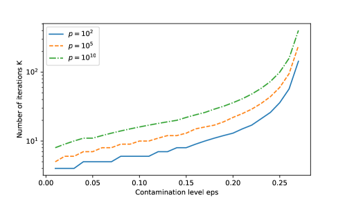
Figure 1: The behavior of the number of iterations $K=K_{\varepsilon}$, given by (15), as a function of the contamination rate $\varepsilon$ for different values of the dimension $p=\textbf{{r}}_{\scriptscriptstyle\boldsymbol{\Sigma}}$.

Note that the value of $K$ provided above is tailored to the case where the initial estimator is the geometric median. Clearly, $K$ depends only logarithmically on the dimension and $K=K_{\varepsilon}$ tends to 2 when $\varepsilon$ goes to zero, see Figure 1. Note also that the choice of $K$ in (15) is derived from the condition $\big{(}\sqrt{\varepsilon(1-\varepsilon)}/(1-2\varepsilon)\big{)}^{K}\|\widehat{\boldsymbol{\mu}}^{0}-\boldsymbol{\mu}^{*}\|_{\mathbf{L}_{2}}\leq\varepsilon$, see (25) below. We can use any other initial estimator of $\boldsymbol{\mu}^{*}$ instead of the geometric median, provided that $K$ is large enough to satisfy the last inequality.

We have to emphasize that $\widehat{\boldsymbol{\mu}}_{n}^{\textup{IR}}$ relies on the knowledge of both $\varepsilon$ and $\boldsymbol{\Sigma}$ (the dependence on $\boldsymbol{\Sigma}$ is through the effective rank, which coincides with the dimension for non degenerate covariance matrices). Indeed, the number of iterations $K$ depends on both $\varepsilon$ and $\boldsymbol{\Sigma}$. Additionally, $\boldsymbol{\Sigma}$ is used in the cost function $G(\boldsymbol{w},\boldsymbol{\mu})$ and $\varepsilon$ is used for specifying the set of feasible weights in optimization problem (14). We present some extensions to the case of unknown $\varepsilon$ and $\boldsymbol{\Sigma}$ in Section 6.

The rest of this section is devoted to showing that the iteratively reweighted estimator enjoys all the desirable properties announced in the introduction. An estimator is called computationally tractable, if its computational complexity is at most polynomial in $n$, $p$ and $1/\varepsilon$.

Fact 1.

f1 The estimator $\widehat{\boldsymbol{\mu}}_{n}^{\textup{IR}}$ is computationally tractable.

In order to check computational tractability, it suffices to prove that each iteration of the algorithm can be performed in polynomial time. Since the number of iterations depends logarithmically on $\textbf{{r}}_{\scriptscriptstyle\boldsymbol{\Sigma}}\leq p$, this will suffice. Note now that the optimization problem in (14) is convex and can be cast into a semi-definite program. Indeed, it is equivalent to minimizing a real value $t$ over all the pairs $(t,\boldsymbol{w})$ satisfying the constraints

$$t\geq 0,\quad\boldsymbol{w}\in\boldsymbol{\Delta}^{n-1},\quad\|\boldsymbol{w}\|_{\infty}\leq\frac{1}{n(1-\varepsilon)},\quad\sum_{i=1}^{n}w_{i}(\boldsymbol{X}_{i}-\widehat{\boldsymbol{\mu}}^{k-1})^{\otimes 2}\preceq\boldsymbol{\Sigma}+t\mathbf{I}_{p}.$$ (16)

The first two constraints can be rewritten as a set of linear inequalities, while the third constraint is a linear matrix inequality. Given the special form of the cost function and the constraints, it is possible to design specific optimization routines which will find an approximate solution to the problem in a faster way than the out-of-shelf SDP-solvers. However, we will not pursue this line of research in this work.

Fact 2.

f2 The estimator $\widehat{\boldsymbol{\mu}}_{n}^{\textup{IR}}$ is translation, uniform scaling and orthogonal transformation equivariant.

The equivariance mentioned in this statement should be understood as follows. If we denote by $\widehat{\boldsymbol{\mu}}_{n,X}^{\textup{IR}}$ the estimator computed for data $\boldsymbol{X}_{1},\ldots,\boldsymbol{X}_{n}$, and by $\widehat{\boldsymbol{\mu}}_{n,X^{\prime}}^{\textup{IR}}$ the one computed for data $\boldsymbol{X}^{\prime}_{1},\ldots,\boldsymbol{X}^{\prime}_{n}$, with $\boldsymbol{X}_{i}^{\prime}=\boldsymbol{a}+\lambda\mathbf{U}\boldsymbol{X}_{i}$, where $\boldsymbol{a}\in\mathbb{R}^{p}$, $\lambda>0$ and $\mathbf{U}$ is a $p\times p$ orthogonal matrix, then $\widehat{\boldsymbol{\mu}}_{n,X^{\prime}}^{\textup{IR}}=\boldsymbol{a}+\lambda\mathbf{U}\widehat{\boldsymbol{\mu}}_{n,X}^{\textup{IR}}$. To prove this property, we first note that

$$\min_{\boldsymbol{\mu}\in\mathbb{R}^{p}}\sum_{i=1}^{n}\|\boldsymbol{X}^{\prime}_{i}-\boldsymbol{\mu}\|_{2}=\lambda\min_{\boldsymbol{\mu}\in\mathbb{R}^{p}}\sum_{i=1}^{n}\|\boldsymbol{X}_{i}-\lambda^{-1}\mathbf{U}^{\top}(\boldsymbol{\mu}-\boldsymbol{a})\|_{2}.$$ (17)

This implies that $\widehat{\boldsymbol{\mu}}_{n,X}^{\textup{GM}}=\lambda^{-1}\mathbf{U}^{\top}(\widehat{\boldsymbol{\mu}}_{n,X^{\prime}}^{\textup{GM}}-\boldsymbol{a})$, which is equivalent to $\widehat{\boldsymbol{\mu}}_{n,X^{\prime}}^{\textup{GM}}=\boldsymbol{a}+\lambda\mathbf{U}\widehat{\boldsymbol{\mu}}_{n,X}^{\textup{GM}}$. Therefore, the initial value of the recursion is equivariant. If we add to this the fact that $G_{X}(\boldsymbol{w},\boldsymbol{\mu})=\lambda^{2}G_{X^{\prime}}(\boldsymbol{w},\boldsymbol{a}+\lambda\mathbf{U}\boldsymbol{\mu})$ for every $(\boldsymbol{w},\boldsymbol{\mu})$, we get the equivariance of $\widehat{\boldsymbol{\mu}}_{n}^{\textup{IR}}$.

Fact 3.

f3 The breakdown point $\varepsilon^{*}_{n}$ and the nearly-minimax-rate-breakdown point $\varepsilon^{*}_{r}$ of $\widehat{\boldsymbol{\mu}}_{n}^{\textup{IR}}$ satisfy, respectively, $\varepsilon^{*}_{n}=0.5$ and $\varepsilon^{*}_{r}\geq(5-\sqrt{5})/10\approx 0.28$.

We prove later in this paper (see (41)) that if $\boldsymbol{X}_{1},\ldots,\boldsymbol{X}_{n}$ satisfy GAC$(\boldsymbol{\mu}^{*},\boldsymbol{\Sigma},\varepsilon)$, there is a random variable $\Xi$ depending only on $\boldsymbol{\zeta}_{i}=\boldsymbol{Y}_{i}-\boldsymbol{\mu}^{*}$, $i=1,\ldots,n$, such that

$$\|\bar{\boldsymbol{X}}_{\boldsymbol{w}}-{\boldsymbol{\mu}}^{*}\|_{2} \leq\frac{\sqrt{\varepsilon(1-\varepsilon)}}{1-2\varepsilon}\,G(\boldsymbol{w},\boldsymbol{\mu})^{1/2}+\Xi,\quad\forall\boldsymbol{\mu}\in\mathbb{R}^{p},$$ (18)

for every $\boldsymbol{w}\in\boldsymbol{\Delta}^{n-1}$ such that $n(1-\varepsilon)\|\boldsymbol{w}\|_{\infty}\leq 1$. Inequality (18) is one of the main building blocks of the proof of LABEL:fact:f3, LABEL:fact:f4 and LABEL:fact:f5. This inequality, as well as inequalities (27) and (28) below will be formally stated and proved in subsequent sections. To check LABEL:fact:f3, we set $\alpha_{\varepsilon}={\sqrt{\varepsilon(1-\varepsilon)}}/{(1-2\varepsilon)}$ and note that

$$\|\widehat{\boldsymbol{\mu}}^{k}-{\boldsymbol{\mu}}^{*}\|_{2}=\|\bar{\boldsymbol{X}}_{\widehat{\boldsymbol{w}}^{k}}-{\boldsymbol{\mu}}^{*}\|_{2} \leq\alpha_{\varepsilon}\,G(\widehat{\boldsymbol{w}}^{k},\widehat{\boldsymbol{\mu}}^{k-1})^{1/2}+\Xi$$ (19)

$$\leq\alpha_{\varepsilon}\,G(\boldsymbol{w}^{*},\widehat{\boldsymbol{\mu}}^{k-1})^{1/2}+\Xi$$ (20)

$$\leq\alpha_{\varepsilon}\,\big{(}G(\boldsymbol{w}^{*},\bar{\boldsymbol{X}}_{\boldsymbol{w}^{*}})+\|\bar{\boldsymbol{X}}_{\boldsymbol{w}^{*}}-\widehat{\boldsymbol{\mu}}^{k-1}\|_{2}^{2}\big{)}^{1/2}+\Xi$$ (21)

$$\leq\alpha_{\varepsilon}\,\big{(}G(\boldsymbol{w}^{*},\boldsymbol{\mu}^{*})+\|\bar{\boldsymbol{X}}_{\boldsymbol{w}^{*}}-\widehat{\boldsymbol{\mu}}^{k-1}\|_{2}^{2}\big{)}^{1/2}+\Xi$$ (22)

$$\leq\alpha_{\varepsilon}\,\|\widehat{\boldsymbol{\mu}}^{k-1}-\boldsymbol{\mu}^{*}\|_{2}+\widetilde{\Xi},$$ (23)

where $\widetilde{\Xi}=\alpha_{\varepsilon}\,\big{(}G(\boldsymbol{w}^{*},\boldsymbol{\mu}^{*})^{1/2}+\|\bar{\boldsymbol{\zeta}}_{\boldsymbol{w}^{*}}\|_{2}\big{)}+\Xi$. Unfolding this recursion, we get

$$\|\widehat{\boldsymbol{\mu}}_{n}^{\textup{IR}}-{\boldsymbol{\mu}}^{*}\|_{2}=\|\widehat{\boldsymbol{\mu}}^{K}-{\boldsymbol{\mu}}^{*}\|_{2} \leq\alpha_{\varepsilon}^{K}\,\|\widehat{\boldsymbol{\mu}}^{0}-\boldsymbol{\mu}^{*}\|_{2}+\frac{\widetilde{\Xi}}{1-\alpha_{\varepsilon}}.$$ (24)

The geometric median $\widehat{\boldsymbol{\mu}}^{0}=\widehat{\boldsymbol{\mu}}_{n}^{\textup{GM}}$ having a breakdown point equal to $1/2$, we infer from the last display that the error of the iteratively reweighted estimator remains bounded after altering $\varepsilon$-fraction of data points provided that $\alpha_{\varepsilon}<1$. This implies that the breakdown point is at least equal to the solution of the equation $\sqrt{\varepsilon(1-\varepsilon)}=1-2\varepsilon$, which yields $\varepsilon^{*}\geq(5-\sqrt{5})/10$. Moreover, if $\varepsilon\in[(5-\sqrt{5})/10,1/2]$, then the number of iterations $K$ equals zero and the iteratively reweighted mean coincides with the geometric median. Therefore, its breakdown point is $1/2$.

Fact 4.

f4 The estimator $\widehat{\boldsymbol{\mu}}_{n}^{\textup{IR}}$ is nearly minimax rate optimal, in the sense that its worst-case risk is bounded by $C\|\boldsymbol{\Sigma}\|^{1/2}_{\textup{op}}\big{(}\sqrt{{\textbf{{r}}_{\scriptscriptstyle\boldsymbol{\Sigma}}}/{n}}+\varepsilon\sqrt{\log(1/\varepsilon)}\big{)}$, where $C$ is a universal constant.

Without loss of generality, we assume that $\|\boldsymbol{\Sigma}\|_{\textup{op}}=1$ so that $\textbf{{r}}_{\scriptscriptstyle\boldsymbol{\Sigma}}=\mathop{\textup{Tr}}(\boldsymbol{\Sigma})$. We can always reduce the initial problem to this case by considering scaled data points $\boldsymbol{X}_{i}/\|\boldsymbol{\Sigma}\|_{\textup{op}}^{1/2}$ instead of $\boldsymbol{X}_{i}$. Combining (24) and the triangle inequality, we get

$$\|\widehat{\boldsymbol{\mu}}_{n}^{\textup{IR}}-{\boldsymbol{\mu}}^{*}\|_{\mathbb{L}_{2}} \leq\alpha_{\varepsilon}^{K}\,\|\widehat{\boldsymbol{\mu}}_{n}^{\textup{GM}}-\boldsymbol{\mu}^{*}\|_{\mathbb{L}_{2}}+\frac{\|\widetilde{\Xi}\|_{\mathbb{L}_{2}}}{1-\alpha_{\varepsilon}}.$$ (25)

It is not hard to check that $\|\widehat{\boldsymbol{\mu}}_{n}^{\textup{GM}}-\boldsymbol{\mu}^{*}\|_{\mathbb{L}_{2}}\leq 2\sqrt{\textbf{{r}}_{\scriptscriptstyle\boldsymbol{\Sigma}}}/(1-2\varepsilon)$, see Lemma 8.11 below. Furthermore, the choice of $K$ in (15) entails $2\alpha_{\varepsilon}^{K}\sqrt{\textbf{{r}}_{\scriptscriptstyle\boldsymbol{\Sigma}}}\leq\varepsilon(1-2\varepsilon)$. This implies that

$$\|\widehat{\boldsymbol{\mu}}_{n}^{\textup{IR}}-{\boldsymbol{\mu}}^{*}\|_{\mathbb{L}_{2}} \leq\varepsilon+\frac{\|\widetilde{\Xi}\|_{\mathbb{L}_{2}}}{1-\alpha_{\varepsilon}}.$$ (26)

The last two building blocks of the proof are the following inequalities:

$$\mathbf{E}[G(\boldsymbol{w}^{*},\boldsymbol{\mu}^{*})]\leq C\big{(}1+\sqrt{\textbf{{r}}_{\scriptscriptstyle\boldsymbol{\Sigma}}/n}\big{)}\sqrt{\textbf{{r}}_{\scriptscriptstyle\boldsymbol{\Sigma}}/n},$$ (27)

$$\|\Xi\|_{\mathbb{L}_{2}}\leq\sqrt{\textbf{{r}}_{\scriptscriptstyle\boldsymbol{\Sigma}}/n}(1+C\sqrt{\varepsilon})+C\sqrt{\varepsilon}(\textbf{{r}}_{\scriptscriptstyle\boldsymbol{\Sigma}}/n)^{1/4}+C\varepsilon\sqrt{\log(1/\varepsilon)},$$ (28)

where $C>0$ is a universal constant. In what follows, the value of $C$ may change from one line to the other. We have

$$\|\widetilde{\Xi}\|_{\mathbb{L}_{2}} \leq\alpha_{\varepsilon}\big{(}\|G(\boldsymbol{w}^{*},\boldsymbol{\mu}^{*})^{1/2}\|_{\mathbb{L}_{2}}+\|\bar{\boldsymbol{\zeta}}_{\boldsymbol{w}^{*}}\|_{\mathbb{L}_{2}}\big{)}+\|\Xi\|_{\mathbb{L}_{2}}$$ (29)

$$\leq C\sqrt{\varepsilon}\,\big{(}\mathbf{E}^{1/2}[G(\boldsymbol{w}^{*},\boldsymbol{\mu}^{*})]+\sqrt{\textbf{{r}}_{\scriptscriptstyle\boldsymbol{\Sigma}}/n}\big{)}+\|\Xi\|_{\mathbb{L}_{2}}^{2}$$ (30)

$$\leq C\varepsilon\,\big{(}(\textbf{{r}}_{\scriptscriptstyle\boldsymbol{\Sigma}}/n)^{1/4}+\sqrt{\textbf{{r}}_{\scriptscriptstyle\boldsymbol{\Sigma}}/n}\big{)}+\|\Xi\|_{\mathbb{L}_{2}}$$ (31)

$$\leq\sqrt{\textbf{{r}}_{\scriptscriptstyle\boldsymbol{\Sigma}}/n}(1+C\sqrt{\varepsilon})+C\sqrt{\varepsilon}(\textbf{{r}}_{\scriptscriptstyle\boldsymbol{\Sigma}}/n)^{1/4}+C\varepsilon\sqrt{\log(1/\varepsilon)}$$ (32)

$$\leq C\sqrt{\textbf{{r}}_{\scriptscriptstyle\boldsymbol{\Sigma}}/n}+C\varepsilon\sqrt{\log(1/\varepsilon)}.$$ (33)

Returning to (24) and combining it with (33), we get the claim of LABEL:fact:f4 for every $\varepsilon\leq\varepsilon_{0}$, where $\varepsilon_{0}$ is any positive number strictly smaller than $(5-\sqrt{5})/10$. This also proves the second claim of LABEL:fact:f3.

Fact 5.

f5 In the setting $\varepsilon=\varepsilon_{n}\to 0$ so that $\varepsilon^{2}\log(1/\varepsilon)=o_{n}(\textbf{{r}}_{\scriptscriptstyle\boldsymbol{\Sigma}}/n)$ when $n\to\infty$, the estimator $\widehat{\boldsymbol{\mu}}_{n}^{\textup{IR}}$ is asymptotically efficient.

The proof of this fact follows from (24) and (28). Indeed, if $\varepsilon^{2}\log(1/\varepsilon)=o_{n}(\textbf{{r}}_{\scriptscriptstyle\boldsymbol{\Sigma}}/n)$, (28) implies that

$$\|\widetilde{\Xi}\|_{\mathbb{L}_{2}}^{2} \leq\frac{\textbf{{r}}_{\scriptscriptstyle\boldsymbol{\Sigma}}}{n}\big{(}1+o_{n}(1)\big{)}.$$ (34)

Injecting this bound in (24) and using the fact that $\varepsilon$ tends to zero, we get the claim of LABEL:fact:f5.

4 Relation to prior work and discussion

Robust estimation of a mean is a statistical problem studied by many authors since at least sixty years. It is impossible to give an overview of all existing results and we will not try to do it here. The interested reader may refer to the books [Maronna et al., 2006] and [Huber and Ronchetti, 2009]. We will rather focus here on some recent results that are the most closely related to the present work. Let us just recall that Huber and Ronchetti [2009] enumerates three desirable properties of a statistical procedure: efficiency, stability and breakdown. We showed here that iteratively reweighted mean estimator possesses these features and, in addition, is equivariant and computationally tractable.

To the best of our knowledge, the form $\sqrt{p/n}+\varepsilon$ of the minimax risk in the Gaussian mean estimation problem has been first obtained by Chen et al. [2018]. They proved that this rate holds with high probability for the Tukey median, which is known to be computationally intractable in the high-dimensional setting. The first nearly-rate-optimal and computationally tractable estimators have been proposed by Lai et al. [2016] and Diakonikolas et al. [2016]. The methods analyzed in these papers are different, but they share the same idea: If for a subsample of points the empirical covariance matrix is sufficiently close to the theoretical one, then the arithmetic mean of this subsample is a good estimator of the theoretical mean. Our method is based on this idea as well, which is mathematically formalized in (18), see also Proposition 5.2 below.

Further improvements in running times—up to obtaining a linear in $np$ computational complexity in the case of a constant $\varepsilon$—are presented in [Cheng et al., 2019a]. Some lower bounds suggesting that the log-factor in the term $\varepsilon\sqrt{\log(1/\varepsilon)}$ cannot be removed from the rate of computationally tractable estimators are established in [Diakonikolas et al., 2017]. In a slightly weaker model of corruption, Diakonikolas et al. [2018] propose an iterative filtering algorithm that achieves the optimal rate $\varepsilon$ without the extra factor $\sqrt{\log(1/\varepsilon)}$. On a related note, [Collier and Dalalyan, 2019] shows that in a weaker contamination model termed as parametric contamination, the carefully trimmed sample mean can achieve a better rate than that of the coordinatewise/geometric median.

An overview of the recent advances on robust estimation with a focus on computational aspects can be found in [Diakonikolas and Kane, 2019]. Extensions of these methods to the sparse mean estimation are developed in [Balakrishnan et al., 2017, Diakonikolas et al., 2019b]. All these results are proved to hold on an event with a prescribed probability, see [Bateni and Dalalyan, 2020] for a relation between results in expectation and those with high probability, as well as for the definitions of various types of contamination.

The proposed estimator shares some features with the adaptive weights smoothing [Polzehl and Spokoiny, 2000]. Adaptive weights smoothing (AWS) iteratively updates the weights assigned to observations, similarly to Algorithm LABEL:algo:a1. The main difference is that the weights in AWS are not measuring the outlyingness but the relevance for interpolating a function at a given point. There are also many other statistical problems in which robust estimation has been recently revisited from the point of view of minimax rates. This includes scale and covariance matrix estimation [Chen et al., 2018, Comminges et al., 2020], matrix completion [Klopp et al., 2017], multivariate regression [Gao, 2020, Dalalyan and Thompson, 2019, Chinot, 2020], classification [Cannings et al., 2020, Li and Bradic, 2018], subspace clustering [Soltanolkotabi and Candès, 2012], community detection [Cai and Li, 2015], etc. Properties of robust $M$-estimators in high-dimensional settings are studied in [Loh, 2017, Elsener and van de Geer, 2018]. There is also an increasing body of literature on the robustness to heavy tailed distributions [Lugosi and Mendelson, 2020, 2019, Devroye et al., 2016, Lecué and Lerasle, 2019, 2020, Minsker, 2018] and the computationally tractable methods in this context [Hopkins, 2018, Cherapanamjeri et al., 2019, Dong et al., 2019, Depersin and Lecué, 2019].

A potentially useful observation, from a computational standpoint, is that it is sufficient to solve the optimization problem in Equation 14 up to an error proportional to $\sqrt{\textbf{{r}}_{\scriptscriptstyle\boldsymbol{\Sigma}}/n}+\sqrt{\varepsilon}$. Indeed, one can easily repeat all the steps in (23) to check that this optimization error does not alter the order of magnitude of the statistical error.

5 Formal statement of main building blocks

The first building block, inequality (18), used in Section 3 to analyze the risk of $\widehat{\boldsymbol{\mu}}^{\textup{IR}}_{n}$, upper bounds the error of estimating the mean by the error of estimating the covariance matrix. In order to formally state the result, we need some additional notations.

Let $\boldsymbol{w}\in\boldsymbol{\Delta}^{n-1}$ be a vector of weights and let $I$ be a subset of $\{1,\ldots,n\}$. We use the notation $\boldsymbol{w}_{I}$ for the vector obtained from $\boldsymbol{w}$ by zeroing all the entries having indices outside $I$. Considering $\boldsymbol{w}$ as a probability on $\{1,\ldots,n\}$, we define $\boldsymbol{w}_{|I}$ as the corresponding conditional probability on $I$ that is

$$\boldsymbol{w}_{|I}\in\boldsymbol{\Delta}^{n-1},\qquad(\boldsymbol{w}_{|I})_{i}=(w_{i}/\|\boldsymbol{w}_{I}\|_{1})\mathds{1}(i\in I).$$ (35)

We will make repeated use of the notation

$$\bar{\boldsymbol{X}}_{\boldsymbol{w}}=\sum_{i=1}^{n}w_{i}\boldsymbol{X}_{i},\qquad\bar{\boldsymbol{\xi}}_{\boldsymbol{w}_{|I}}=\sum_{i\in I}(\boldsymbol{w}_{|I})_{i}\boldsymbol{\xi}_{i},\qquad\bar{\boldsymbol{\zeta}}_{\boldsymbol{w}_{|I}}=\sum_{i\in I}(\boldsymbol{w}_{|I})_{i}\boldsymbol{\zeta}_{i}.$$ (36)

Proposition 5.2.

Let $\boldsymbol{\zeta}_{1},\ldots,\boldsymbol{\zeta}_{n}$ be a set of vectors such that $\boldsymbol{\zeta}_{i}=\boldsymbol{X}_{i}-\boldsymbol{\mu}^{*}$ for every $i\in\mathcal{I}$, where $\mathcal{I}$ is a subset of $\{1,\ldots,n\}$. For every weight vector $\boldsymbol{w}\in\boldsymbol{\Delta}^{n-1}$ such that $\sum_{i\not\in\mathcal{I}}w_{i}\leq\varepsilon_{w}\leq 1/2$ and for every $p\times p$ matrix $\boldsymbol{\Sigma}$, it holds

$$\|\bar{\boldsymbol{X}}_{\boldsymbol{w}}-{\boldsymbol{\mu}}^{*}\|_{2} \leq\frac{\sqrt{\varepsilon_{w}}}{1-\varepsilon_{w}}\,\lambda_{\max,+}^{1/2}\Big{(}\sum_{i=1}^{n}w_{i}(\boldsymbol{X}_{i}-\bar{\boldsymbol{X}}_{\boldsymbol{w}})^{\otimes 2}-\boldsymbol{\Sigma}\Big{)}+R(\boldsymbol{\zeta},\boldsymbol{w},\mathcal{I}),$$ (37)

with the remainder term

$$R(\boldsymbol{\zeta},\boldsymbol{w},\mathcal{I})=2\sqrt{\|\boldsymbol{\Sigma}\|_{\rm op}}\varepsilon_{w}+\sqrt{2\varepsilon_{w}}\,\lambda_{\max,+}^{1/2}\bigg{(}\sum_{i\in\mathcal{I}}(\boldsymbol{w}_{|\mathcal{I}})_{i}(\boldsymbol{\Sigma}-\boldsymbol{\zeta}_{i}\boldsymbol{\zeta}_{i}^{\top})\bigg{)}+(1+\sqrt{2\varepsilon_{w}})\|\bar{\boldsymbol{\zeta}}_{\boldsymbol{w}_{|\mathcal{I}}}\|_{2}.$$ (38)

The proof of this result is postponed to the last section. In simple words, the claim of proposition is that the estimation error of the weighted mean $\bar{\boldsymbol{X}}_{\boldsymbol{w}}$ is, up to a remainder term, governed by the quantity $G(\boldsymbol{w},\bar{\boldsymbol{X}}_{\boldsymbol{w}})^{1/2}$. It turns out that the remainder term is bounded by a small quantity uniformly in $\boldsymbol{w}$ and $\mathcal{I}$, provided that these two satisfy suitable conditions. For $\mathcal{I}$, it is enough to constrain the cardinality of its complement $\mathcal{I}^{c}=\mathcal{O}$. For $\boldsymbol{w}$, it appears to be sufficient to assume that its sup-norm is small. In that respect, the following lemma plays a key role in the proof.

Lemma 5.3.

For any integer $\ell>0$, let $\mathcal{W}_{n,\ell}$ be the set of all $\boldsymbol{w}\in\boldsymbol{\Delta}^{n-1}$ such that $\max_{i}w_{i}\leq 1/\ell$. The following facts hold:

1. For every $J\subset\{1,\ldots,n\}$ such that $|J|\geq\ell$, the uniform weight vector $\boldsymbol{u}^{J}\in\mathcal{W}_{n,\ell}$.

2. The set $\mathcal{W}_{n,\ell}$ is the convex hull of the uniform weight vectors $\{\boldsymbol{u}^{J}:|J|=\ell\}$.

3. For every convex mapping $G:\boldsymbol{\Delta}^{n-1}\to\mathbb{R}$, we have

   $$\sup_{\boldsymbol{w}\in\mathcal{W}_{n,\ell}}G(\boldsymbol{w})=\max_{|J|=\ell}G(\boldsymbol{u}^{J}),$$ (39)

   where the last maximum is over all subsets $J$ of cardinality $\ell$ of the set $\{1,\ldots,n\}$.

4. If $\boldsymbol{w}\in\mathcal{W}_{n,\ell}$ then for any $I$ such that $|I|\geq\ell^{\prime}>n-\ell$, we have $\boldsymbol{w}_{|I}\in\mathcal{W}_{n,\ell+\ell^{\prime}-n}$.

Let us denote by $\mathcal{W}_{n}(\varepsilon)$ the set $\mathcal{W}_{n,n(1-\varepsilon)}$. This is exactly the feasible set in the optimization problem defining the iterations of Algorithm LABEL:algo:a1. It is clear that for $\boldsymbol{w}\in\mathcal{W}_{n}(\varepsilon)$ and for $|I^{c}|\leq n\varepsilon$, we have $\sum_{i\not\in I}w_{i}\leq\varepsilon/(1-\varepsilon)$. We now infer from Proposition 5.2 and (12) that

$$\|\bar{\boldsymbol{X}}_{\boldsymbol{w}}-{\boldsymbol{\mu}}^{*}\|_{2} \leq\alpha_{\varepsilon}\,\lambda_{\max,+}^{1/2}\Big{(}\sum_{i=1}^{n}w_{i}(\boldsymbol{X}_{i}-\bar{\boldsymbol{X}}_{\boldsymbol{w}})^{\otimes 2}-\boldsymbol{\Sigma}\Big{)}+\Xi$$ (40)

$$=\alpha_{\varepsilon}\,\inf_{\boldsymbol{\mu}\in\mathbb{R}^{p}}G(\boldsymbol{w},\boldsymbol{\mu})^{1/2}+\Xi,$$ (41)

with $\Xi$ being the largest value of $R(\boldsymbol{\zeta},\boldsymbol{w},I)$ over all possible weights $\boldsymbol{w}\in\mathcal{W}_{n}(\varepsilon)$ and subsets $I\subset\{1,\ldots,n\}$ satisfying $|I^{c}|\leq n\varepsilon$. The second building block, formally stated in the next proposition, provides a suitable upper bound for the random variable $\Xi$.

Proposition 5.4.

Let $R(\boldsymbol{\zeta},\boldsymbol{w},I)$ be defined in Proposition 5.2 and $\boldsymbol{\zeta}_{1},\ldots,\boldsymbol{\zeta}_{n}$ be i.i.d. centered Gaussian random vectors with covariance matrix $\boldsymbol{\Sigma}$ satisfying $\lambda_{\max}(\boldsymbol{\Sigma})=1$. If $\varepsilon\leq 0.28$, then the random variable

$$\Xi=\sup_{\boldsymbol{w}\in\mathcal{W}_{n}(\varepsilon)}\max_{|I|\geq n(1-\varepsilon)}R(\boldsymbol{\zeta},\boldsymbol{w},I)$$ (42)

satisfies, for a universal constant $C>0$, the inequalities

$$\|\Xi\|_{\mathbb{L}_{2}} \leq\sqrt{\textbf{{r}}_{\scriptscriptstyle\boldsymbol{\Sigma}}/n}(1+C\sqrt{\varepsilon})+C\sqrt{\varepsilon}(\textbf{{r}}_{\scriptscriptstyle\boldsymbol{\Sigma}}/n)^{1/4}+C\varepsilon\sqrt{\log(1/\varepsilon)}$$ (43)

$$\|\Xi\|_{\mathbb{L}_{2}} \leq\sqrt{p/n}(1+16\sqrt{\varepsilon})+5\sqrt{3\varepsilon}\,(p/n)^{1/4}+32\varepsilon\sqrt{\log(2/\varepsilon)},$$ (44)

where for the second inequality we assumed that $p\geq 2$ and $n\geq p\vee 4$.

The second inequality is weaker than the first one, since obviously $\textbf{{r}}_{\scriptscriptstyle\boldsymbol{\Sigma}}\leq p$. However, the advantage of the second inequality is that it comes with explicit constants and shows that these constants are not excessively large.

To close this section, we state a theorem that rephrases LABEL:fact:f4 in a way that might be more convenient for future references. Its proof is omitted, since it follows the lines of the proof of LABEL:fact:f4 presented above.

Theorem 5.5.

Let $\widehat{\boldsymbol{\mu}}_{n}^{\textup{IR}}$ be the iteratively reweighted mean defined in Definition 3.1 and Algorithm LABEL:algo:a1. There is a universal constant $C>0$ such that for any $n,p\geq 1$ and for every $\varepsilon<(5-\sqrt{5})/10$, we have

$$\sup_{\boldsymbol{\mu}^{*}\in\mathbb{R}^{p}}\sup_{\mathbf{P}\!_{n}\in\textup{GAC}(\boldsymbol{\mu}^{*},\boldsymbol{\Sigma},\varepsilon)}\mathbf{E}^{1/2}[\|\widehat{\boldsymbol{\mu}}_{n}^{\textup{IR}}-\boldsymbol{\mu}^{*}\|_{2}^{2}]\leq\frac{C\|\boldsymbol{\Sigma}\|^{1/2}_{\textup{op}}}{1-2\varepsilon-\sqrt{\varepsilon(1-\varepsilon)}}\,\big{(}\sqrt{\textbf{{r}}_{\scriptscriptstyle\boldsymbol{\Sigma}}/n}+\varepsilon\sqrt{\log(1/\varepsilon)}\big{)},$$ (45)

where $\mathbf{P}\!_{n}\in\textup{GAC}(\boldsymbol{\mu}^{*},\boldsymbol{\Sigma},\varepsilon)$ means that the data points $\boldsymbol{X}_{i}$ are Gaussian with adversarial contamination, see Definition 1. If, in addition, $p\geq 2$ and $n\geq p\vee 10$, then

$$\sup_{\boldsymbol{\mu}^{*}\in\mathbb{R}^{p}}\sup_{\mathbf{P}\!_{n}\in\textup{GAC}(\boldsymbol{\mu}^{*},\boldsymbol{\Sigma},\varepsilon)}\mathbf{E}^{1/2}[\|\widehat{\boldsymbol{\mu}}_{n}^{\textup{IR}}-\boldsymbol{\mu}^{*}\|_{2}^{2}]\leq\frac{10\|\boldsymbol{\Sigma}\|^{1/2}_{\textup{op}}}{1-2\varepsilon-\sqrt{\varepsilon(1-\varepsilon)}}\,\big{(}\sqrt{p/n}+\varepsilon\sqrt{\log(1/\varepsilon)}\big{)}.$$ (46)

To the best of our knowledge, this is the first result in the literature that provides an upper bound on the expected error of an outlier-robust estimator, which is of nearly optimal rate.

6 Sub-Gaussian distributions, high-probability bounds and adaptation

Risk bounds stated in LABEL:fact:f4 and LABEL:fact:f5 and formalized in Theorem 5.5 hold for the expected error under the condition that the reference distribution is Gaussian. Furthermore, the proposed procedure relies on the knowledge of both the contamination rate $\varepsilon$ and the covariance matrix $\mathbf{\Sigma}$. The goal of this section is to show how some of these restriction can be alleviated.

6.1 High-probability risk bound for a sub-Gaussian reference distribution

As expected, the risk bounds established in previous sections can be extended to the case of sub-Gaussian distributions. Furthermore, risk bounds holding with high-probability can be proved using the same techniques as those employed for proving the in-expectation bounds. In order to be more precise, we state in this subsection the high-probability counterpart of the second claim of Theorem 5.5. The price to pay for covering the more general sub-Gaussian case is that the constant in the right hand side of the inequality is no longer explicit.

Recall that a zero-mean random vector $\boldsymbol{\xi}$ is called sub-Gaussian with parameter $\tau>0$ (also known as the variance proxy), if

$$\mathbf{E}[e^{\boldsymbol{v}^{\top}\boldsymbol{\xi}}]\leq e^{\nicefrac{{\tau}}{{2}}\|\boldsymbol{v}\|_{2}^{2}},\qquad\forall\boldsymbol{v}\in\mathbb{R}^{p}.$$ (47)

We write $\boldsymbol{\xi}\sim SG_{p}(\tau)$. If $\boldsymbol{\xi}$ is standard Gaussian then it is sub-Gaussian with parameter $1$. Similarly, if $\boldsymbol{\xi}$ is centered and belongs almost surely to the unit ball, then $\boldsymbol{\xi}$ is sub-Gaussian with parameter 1. Let us describe now the set of data-generating distributions that we consider in this section.

Definition 6.6.

We say that the joint distribution $\mathbf{P}\!_{n}$ of the random vectors $\boldsymbol{X}_{1},\ldots,\boldsymbol{X}_{n}\in\mathbb{R}^{p}$ belongs to the sub-Gaussian model with adversarial contamination with mean $\boldsymbol{\mu}^{*}$, covariance matrix $\boldsymbol{\Sigma}$ and contamination rate $\varepsilon$, if there are independent random vectors $\boldsymbol{\xi}_{i}\sim SG_{p}(\tau)$ such that

$$\Big{|}\Big{\{}i:=1,\ldots,n:\boldsymbol{X}_{i}\neq\boldsymbol{\mu}^{*}+\boldsymbol{\Sigma}^{1/2}\boldsymbol{\xi}_{i}\Big{\}}\Big{|}\leq\varepsilon n.$$ (48)

We then write $\mathbf{P}\!_{n}\in\textup{SGAC}(\boldsymbol{\mu}^{*},\boldsymbol{\Sigma},\varepsilon)$.

It is clear that a Gaussian model with adversarial contamination defined in Definition 1 is a particular case of the sub-Gaussian model with adversarial contamination. In other terms, the set SGAC$(\boldsymbol{\mu}^{*},\boldsymbol{\Sigma},\varepsilon)$ is strictly larger than the set GAC$(\boldsymbol{\mu}^{*},\boldsymbol{\Sigma},\varepsilon)$. Nevertheless, as shows the result below, the risk bounds established for the iteratively reweighted mean algorithms remain valid uniformly over this extended class SGAC$(\boldsymbol{\mu}^{*},\boldsymbol{\Sigma},\varepsilon)$.

Theorem 6.7.

Let $\widehat{\boldsymbol{\mu}}_{n}^{\textup{IR}}$ be the iteratively reweighted mean defined in Definition 3.1 and in Algorithm LABEL:algo:a1. Let $\delta\in(4e^{-n},1)$ be a tolerance level. There exists a constant $A_{5}$ depending only on the variance proxy $\tau$ such that if $n\geq p\geq 2$ and $\varepsilon<(5-\sqrt{5})/10$, then for every $\boldsymbol{\mu}^{*}\in\mathbb{R}^{p}$ and every $\mathbf{P}\!_{n}\in\textup{SGAC}(\boldsymbol{\mu}^{*},\boldsymbol{\Sigma},\varepsilon)$, we have

$$\mathbf{P}\Bigg{(}\|\widehat{\boldsymbol{\mu}}_{n}^{\textup{IR}}-\boldsymbol{\mu}^{*}\|_{2}^{2}\leq\frac{A_{5}\|\boldsymbol{\Sigma}\|^{1/2}_{\textup{op}}}{1-2\varepsilon-\sqrt{\varepsilon(1-\varepsilon)}}\,\bigg{(}\sqrt{\frac{p+\log(4/\delta)}{n}}+\varepsilon\sqrt{\log(1/\varepsilon)}\bigg{)}\Bigg{)}\leq 1-4\delta.$$ (49)

The proof of this theorem is postponed to the supplementary material. Let us just mention that [Cheng et al., 2019b, Section 1.2] claim that the rate $\sqrt{p/n}+\varepsilon\sqrt{\log(1/\varepsilon)}$ is optimal for sub-Gaussian distributions, meaning that, unlike the Gaussian case, the $\sqrt{\log(1/\varepsilon)}$ factor cannot be removed. A formal proof of this fact can be found in the last remark of Section 2 in [Lugosi and Mendelson, 2021].

6.2 Adaptation to unknown contamination rate $\varepsilon$

An appealing feature of the risk bounds that hold with high probability is that they allow us to apply Lepski’s method [Lepskii, 1992, Lepski and Spokoiny, 1997] for obtaining an adaptive estimator with respect to $\varepsilon$. The obtained adaptive estimator enjoys all the five properties enumerated in Section 3 except the asymptotic efficiency, since the adaptation results in an inflation of the risk bound by a factor 3. The precise description of the algorithm, already used in the framework of robust estimation by Collier and Dalalyan [2019], is presented below. We will denote by $\mathbb{B}(\boldsymbol{\mu},r)$ the ball with center $\boldsymbol{\mu}$ and radius $r$ in the Euclidean space $\mathbb{R}^{p}$.

Definition 6.8.

We choose a geometric grid $\varepsilon_{\ell}=a^{\ell}\varepsilon_{0}$, $\ell=1,2,\ldots,\ell_{\max}$, of possible values of the contamination rate. Here, $a\in(0,1)$ is a real number, $\varepsilon_{0}=(5-\sqrt{5})/10$ and $\ell_{\max}=[0.5\log_{a}(p/n)]$. For each $\ell=1,\ldots,\ell_{\max}$, we denote by $\widehat{\boldsymbol{\mu}}_{n}^{\textup{IR}}(\varepsilon_{\ell})$ the iteratively reweighted mean computed for $\varepsilon=\varepsilon_{\ell}$, see Algorithm LABEL:algo:a1, and we set

$$R_{\delta}(z)=\frac{A_{5}\|\boldsymbol{\Sigma}\|^{1/2}_{\textup{op}}}{1-2z-\sqrt{z(1-z)}}\,\bigg{(}\sqrt{\frac{p+\log(4\ell_{\max}/\delta)}{n}}+z\sqrt{\log(1/z)}\bigg{)},\qquad z\in[0,\varepsilon_{0}),$$ (50)

where $\delta\in(0,1)$ is a tolerance level and $A_{5}$ is the constant from Theorem 6.7. The adaptively chosen iteratively reweighted mean estimator $\widehat{\boldsymbol{\mu}}_{n}^{\textup{AIR}}$ is defined by $\widehat{\boldsymbol{\mu}}_{n}^{\textup{AIR}}=\widehat{\boldsymbol{\mu}}_{n}^{\textup{IR}}(\varepsilon_{\widehat{\ell}})$ where

$$\widehat{\ell}=\max\Big{\{}\ell\leq\ell_{\max}:\bigcap_{j=1}^{\ell}\mathbb{B}\big{(}\widehat{\boldsymbol{\mu}}_{n}^{\textup{IR}}(\varepsilon_{j});R_{\delta}(\varepsilon_{j})\big{)}\neq\varnothing\Big{\}}.$$ (51)

The estimator $\widehat{\boldsymbol{\mu}}_{n}^{\textup{AIR}}$ can be computed without the knowledge of the true contamination rate $\varepsilon$. Furthermore, its computational complexity nearly of the same order as the complexity of computing a single instance of the iteratively reweighted mean as defined by Algorithm LABEL:algo:a1. Indeed, to compute $\widehat{\boldsymbol{\mu}}_{n}^{\textup{AIR}}$, one needs to apply Algorithm LABEL:algo:a1 at most $\ell_{\max}=[0.5\log_{a}(p/n)]$ times, and to solve a second-order cone program for checking whether the intersection of a small number of balls is empty. The next theorem, proved in the supplementary material, shows that the estimation error of this estimator $\widehat{\boldsymbol{\mu}}_{n}^{\textup{AIR}}$ is of the optimal rate, up to a logarithmic factor. To the best of our knowledge, this is the first result of this kind in the literature.

Theorem 6.9.

Let $\widehat{\boldsymbol{\mu}}_{n}^{\textup{AIR}}$ be the estimator defined in Definition 6.8. Let $\delta\in(4e^{-n},1)$ be a tolerance level. Let $n\geq p\geq 2$ and $\varepsilon\leq(5-\sqrt{5})a/10$, where $a\in(0,1)$ is the parameter used in Definition 6.8. Then, for every $\boldsymbol{\mu}^{*}\in\mathbb{R}^{p}$ and every $\mathbf{P}\!_{n}\in\textup{SGAC}(\boldsymbol{\mu}^{*},\boldsymbol{\Sigma},\varepsilon)$, we have

$$\mathbf{P}\Bigg{(}\|\widehat{\boldsymbol{\mu}}_{n}^{\textup{AIR}}-\boldsymbol{\mu}^{*}\|_{2}^{2}\leq\frac{3A_{5}\|\boldsymbol{\Sigma}\|^{1/2}_{\textup{op}}}{a-2\varepsilon-\sqrt{\varepsilon(a-\varepsilon)}}\,\bigg{(}\sqrt{\frac{p+\log(4\ell_{\max}/\delta)}{n}}+\varepsilon\sqrt{\log(1/\varepsilon)}\bigg{)}\Bigg{)}\leq 1-4\delta.$$ (52)

The breakdown point of the adaptive estimator $\widehat{\boldsymbol{\mu}}_{n}^{\textup{AIR}}$ inferred from the last theorem is slightly smaller than the one of $\widehat{\boldsymbol{\mu}}_{n}^{\textup{IR}}$. Indeed, there is a factor $a<1$ between these two quantities. Note that one can choose $a$ to be very close to one. The only drawback of choosing $a$ too close to one is the higher computational complexity of the resulting estimator.

Algorithm 2.

Iteratively reweighted mean estimator (known $\boldsymbol{\varepsilon}$, unknown $\boldsymbol{\Sigma}$)a2

  Input: data $\boldsymbol{X}_{1},\ldots,\boldsymbol{X}_{n}\in\mathbb{R}^{p}$, contamination rate $\varepsilon$

  Output: parameter estimate $\widehat{\boldsymbol{\mu}}_{n}^{\textup{IR}}$

  Initialize: compute $\widehat{\boldsymbol{\mu}}^{0}$ as a minimizer of $\sum_{i=1}^{n}\|\boldsymbol{X}_{i}-\boldsymbol{\mu}\|_{2}$

  Set $K=0\vee\Big{\lceil}\frac{\log(4p)-2\log(\varepsilon({1-2\varepsilon}))}{2\log(1-2\varepsilon)-\log\varepsilon-\log(1-\varepsilon)}\Big{\rceil}$.

  For $k=1:K$

    Compute current weights:   $\displaystyle\boldsymbol{w}\in\mathop{\textup{arg\,min}}_{(n-n\varepsilon)\|\boldsymbol{w}\|_{\infty}\leq 1}\lambda_{\max}\bigg{(}\sum_{i=1}^{n}w_{i}(\boldsymbol{X}_{i}-\widehat{\boldsymbol{\mu}}^{k-1})^{\otimes 2}\bigg{)}.$

    Update the estimator: $\widehat{\boldsymbol{\mu}}^{k}=\sum_{i=1}^{n}w_{i}\boldsymbol{X}_{i}$.

  EndFor

  Return $\widehat{\boldsymbol{\mu}}^{K}$.

6.3 Extension to unknown covariance $\mathbf{\Sigma}$

The iteratively reweighted mean estimator, as defined in Algorithm LABEL:algo:a1, requires the knowledge of the covariance matrix $\boldsymbol{\Sigma}$. Let us briefly discuss what happens when this matrix is unknown, by considering two qualitatively different situations.

The first situation is when the covariance matrix is isotropic, $\boldsymbol{\Sigma}=\sigma^{2}\mathbf{I}_{p}$, with unknown $\sigma>0$. One can easily check that all the claims of Section 3 and Section 5 hold true for a slight modification of $\widehat{\mu}_{n}^{\textup{IR}}$ obtained by minimizing $\lambda_{\max}(\sum_{i}w_{i}(\boldsymbol{X}_{i}-\widehat{\mu}^{k-1})^{\otimes 2}-\boldsymbol{\Sigma})$ instead of $G(\boldsymbol{w},\widehat{\boldsymbol{\mu}}^{k-1})$ in (14). For isotropic matrices $\boldsymbol{\Sigma}$, we have

$$\text{arg}\min_{\boldsymbol{w}}\lambda_{\max}\bigg{(}\sum_{i}w_{i}(\boldsymbol{X}_{i}-\widehat{\mu}^{k-1})^{\otimes 2}-\sigma^{2}\mathbf{I}_{p}\bigg{)}=\text{arg}\min_{\boldsymbol{w}}\lambda_{\max}\bigg{(}\sum_{i}w_{i}(\boldsymbol{X}_{i}-\widehat{\mu}^{k-1})^{\otimes 2}\bigg{)},$$ (53)

which means that the resulting value is independent of $\boldsymbol{\Sigma}$. Therefore, in this first situation, the modified estimator defined in Algorithm LABEL:algo:a2 satisfies inequalities of Theorem 5.5 and Theorem 6.7.

The second situation is when $\boldsymbol{\Sigma}$ is unknown and arbitrary. In this case, to the best of our knowledge, there is no known computationally tractable estimator of $\boldsymbol{\mu}^{*}$ achieving a rate faster than $\sqrt{p/n}+\sqrt{\varepsilon}$. It turns out that a slightly modified version of the iteratively reweighted mean estimator defined in Algorithm LABEL:algo:a2 achieves this rate as well. The formal statement of the result entailing this claim is presented below.

Theorem 6.10.

Let $\widehat{\boldsymbol{\mu}}_{n}^{\textup{IR}}$ be the iteratively reweighted mean defined in Algorithm LABEL:algo:a2. Let $\delta\in(4e^{-n},1)$ be a tolerance level. There exists a constant $A_{5}$ depending only on the variance proxy $\tau$ such that if $n\geq p\geq 2$ and $\varepsilon<(5-\sqrt{5})/10$, then for every $\boldsymbol{\mu}^{*}\in\mathbb{R}^{p}$ and every $\mathbf{P}\!_{n}\in\textup{SGAC}(\boldsymbol{\mu}^{*},\boldsymbol{\Sigma},\varepsilon)$, we have

$$\mathbf{P}\Bigg{(}\|\widehat{\boldsymbol{\mu}}_{n}^{\textup{IR}}-\boldsymbol{\mu}^{*}\|_{2}^{2}\leq\frac{A_{5}\|\boldsymbol{\Sigma}\|^{1/2}_{\textup{op}}}{1-2\varepsilon-\sqrt{\varepsilon(1-\varepsilon)}}\,\bigg{(}\sqrt{\frac{p+\log(4/\delta)}{n}}+3\sqrt{\varepsilon}\bigg{)}\Bigg{)}\leq 1-4\delta.$$ (54)

The proof of this theorem is deferred to the supplementary material. One can use Theorem 6.10 to construct an adaptive (with respect to $\varepsilon$) estimator of $\boldsymbol{\mu}^{*}$ in the case of unknown $\boldsymbol{\Sigma}$ using Lepski’s method detailed in Section 6.2. For this construction, it suffices to know an upper bound $\sigma_{\max}$ on the operator norm $\|\boldsymbol{\Sigma}\|^{1/2}_{\textup{op}}$. The resulting estimator has an error of the order $\sigma_{\max}(\sqrt{p/n}+\sqrt{\varepsilon})$.

One can also consider intermediate cases, in which the covariance matrix is not arbitrary but has a more general form than the simple isotropic one. In such a situation, it might be of interest to extend the method proposed in Algorithm LABEL:algo:a1 by using an initial estimator of $\boldsymbol{\Sigma}$ and by updating its value at each step. Indeed, when a weight vector is computed, it can be used for updating not only the mean but also the covariance matrix. The study of this estimator is left for future research.

7 Empirical results

This section showcases empirical results obtained by applying the iteratively reweighted mean estimator described in Algorithm LABEL:algo:a1 to synthetic data sets. We stress right away that there are multiple ways of solving the optimization problem involved in Algorithm LABEL:algo:a1, and the implementation we used in our experiments is not the most efficient one. As already mentioned, the aforementioned optimization problem can be seen as a semi-definite program and out-of-shelf algorithm can be applied to solve it. We implemented this approach in R using the MOSEK solver. All the results reported in this section are obtained using this implementation. We are currently working on an improved implementation using the dual sub-gradient algorithm of [Cox et al., 2014].

We applied Algorithm LABEL:algo:a1 to $\boldsymbol{X}_{1},\dots,\boldsymbol{X}_{n}$ from $\mathbf{P}\!_{n}\in\textup{GAC}(\boldsymbol{\mu}^{*},\boldsymbol{\Sigma},\varepsilon)$ with various types of contamination schemes. In the numerical experiments below, we illustrate (a) the evolution of the estimation error along the iterations, (b) the properties related to the theoretical breakdown point and (c) the performance of the estimator obtained from Algorithm LABEL:algo:a1 as compared to some simple estimators of the mean and to the oracle. In this section, the error of estimation is understood as the Euclidean distance between the estimated mean and its true value.

Notice that, due to the equivariance stated in LABEL:fact:f2, it is sufficient to take as the true target mean vector $\boldsymbol{\mu}^{*}$ the zero vector $\mathbf{0}_{p}$ and as $\boldsymbol{\Sigma}$ any diagonal matrix with nonnegative entries. We consider the following two schemes of outlier generation:

• Contamination by “smallest” eigenvector: Sample $n$ i.i.d. observations $\boldsymbol{Y}_{1},\dots,\boldsymbol{Y}_{n}$ drawn from $\mathcal{N}(\mathbf{0}_{p},\mathbf{I}_{p})$ and compute the smallest eigenvalue $\lambda_{p}$ and the corresponding eigenvector $\boldsymbol{v}_{p}$ of the sample covariance matrix, defined as

  $$\widehat{\boldsymbol{\Sigma}}_{n}=\frac{1}{n}\sum_{i=1}^{n}(\boldsymbol{Y}_{i}-\overline{\boldsymbol{Y}}_{n})^{\otimes 2},$$ (55)

  where $\overline{\boldsymbol{Y}}_{n}\stackrel{{\scriptstyle\text{def}}}{{=}}(\boldsymbol{Y}_{1}+\dots+\boldsymbol{Y}_{n})/n$. Choose the ${n\varepsilon}$ observations from $\boldsymbol{Y}_{1},\dots,\boldsymbol{Y}_{n}$ that have the highest (in absolute value) correlation coefficient with $\boldsymbol{v}_{p}$ and replace them by a vector proportional to $\boldsymbol{v}_{p}$ with proportionality coefficient equal to $\sqrt{p}$.

• Uniform outliers: Sample $n$ observations according to this model

  $$\boldsymbol{Y}_{i}=\boldsymbol{\theta}_{i}+\boldsymbol{\xi}_{i},\text{ with }\boldsymbol{\xi}_{i}\stackrel{{\scriptstyle\text{i.i.d.}}}{{\sim}}\mathcal{N}(\mathbf{0}_{p},\mathbf{I}_{p})\text{ for }~{}i=1,\dots,n,$$ (56)

  where $\boldsymbol{\theta}_{i}$s are all-zero vectors for $n(1-\varepsilon)$ observations $i\in\mathcal{I}=\{1,\ldots,n(1-\varepsilon)\}$, while for the indices $i\not\in\mathcal{I}$ we have $\|\boldsymbol{\theta}_{i}\|_{2}\neq 0$. We take the values of $\{\boldsymbol{\theta}_{i}\}_{i\in\mathcal{O}}$ to be i.i.d. from uniform distribution, i.e., for $i\not\in\mathcal{I}$ we take $\{\boldsymbol{\theta}_{i}^{j}\}_{j=1}^{p}\stackrel{{\scriptstyle\text{i.i.d.}}}{{\sim}}\mathcal{U}[a,b]$. We took different values of $a$ and $b$ in different experiments reported below.

7.1 Improvement along iterations

In this experiment we show the improvement of the estimation error along the iterations. The data for this experiment were generated according to the second contamination scheme mentioned above with $a=0.5$ and $b=2$. In Figure 3, we drew the logarithm of the estimation error (i.e., the risk between $\widehat{\boldsymbol{\mu}}_{n}$ and $\boldsymbol{\mu}^{*}$) as a function of the iteration number. The results are obtained by averaging over 50 independent repetitions. We observe that the error decreases very fast during the first iteration and remains almost constant during the rest of time. As a matter of fact, in order to speed-up the procedure, we can stop the iterations if the current weights $\boldsymbol{w}$ satisfy $\lambda_{\max}(\sum_{i}w_{i}(\boldsymbol{X}_{i}-\bar{\boldsymbol{X}}_{\boldsymbol{w}})^{\otimes 2}-\boldsymbol{\Sigma})\leq\varepsilon$. It is easy to check that this modified estimator still possesses all the desirable properties described in previous sections.

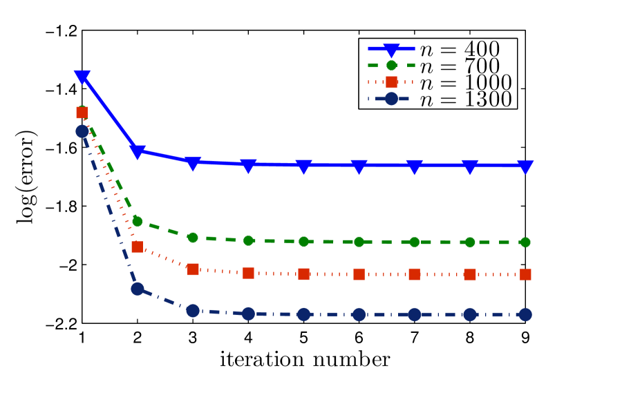
Figure 2: The decay of the error along the iterations for $p=9$, $\varepsilon=0.2$ and different values of $n$. The contamination scheme is “uniform outliers” with $(a,b)=(0.5,2)$.

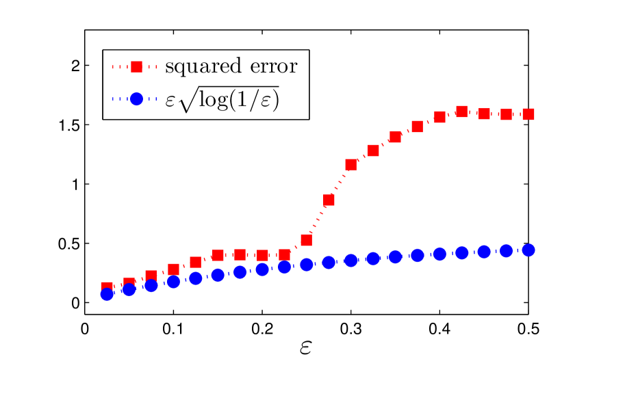
Figure 3: The error as a function of the contamination rate $\varepsilon$ for $n=500$ and $p=5$. The contamination scheme is “smallest” eigenvector. The number of iterations for $\varepsilon>\varepsilon^{*}$ was set to $30$.

7.2 Breakdown point

The goal of this experiment is to check empirically the validity of the breakdown point $\varepsilon^{*}\stackrel{{\scriptstyle\text{def}}}{{=}}(5-\sqrt{5})/10\approx 0.28$. To this end, we chose to contaminate the standard normal vectors by “smallest” eigenvector scheme. Note that if the outliers are well separated from the inliers, like in the uniform outliers scheme, then Algorithm LABEL:algo:a1 detects well these outliers by pushing their weights to $0$ even when $\varepsilon$ is large (larger than $0.28$).

For $n=500$ and $p=5$, we conducted 50 independent repetitions of the experiment and plotted the error averaged over these 50 repetitions in Figure 3. For $\varepsilon>0.28$, we manually set the number of iterations to 30. It is interesting to observe that there is a clear change in the mean error occurring at a value close to $0.28$. This empirical result allows us to conjecture that the breakdown point of the presented estimator is indeed close to $0.28$.

7.3 Comparison with other estimators

In this last experiment we wanted to provide a visual illustration of the performance of the proposed estimator $\widehat{\boldsymbol{\mu}}^{\text{IR}}_{n}$ as compared to some simple competitors: the sample mean, the coordinatewise median, the geometric median and the oracle obtained by averaging all the inliers. The obtained errors, averaged over 50 independent repetitions, are depicted in Figure 5 and Figure 5. The former corresponds to $n=500$, $p=20$ and varying $\varepsilon$, while the parameters of the latter are $p=10$, $\varepsilon=0.1$ and $n\in[10,1000]$. In the legend of these figures, Estimated Mu refers to $\widehat{\boldsymbol{\mu}}^{\text{IR}}_{n}$, the output of Algorithm LABEL:algo:a1, Sample Mean and Sample Median correspond respectively to the sample mean and sample coordinatewise median, Geometric Median refers to the estimator defined in (13) and Oracle refers to the sample mean of inliers only.

The plots show that the iteratively reweighted mean estimators has an error which is nearly as small as the error of the oracle. These errors are way smaller than the errors of the other estimators included in this experiment, which is in line with all the existing theoretical results.

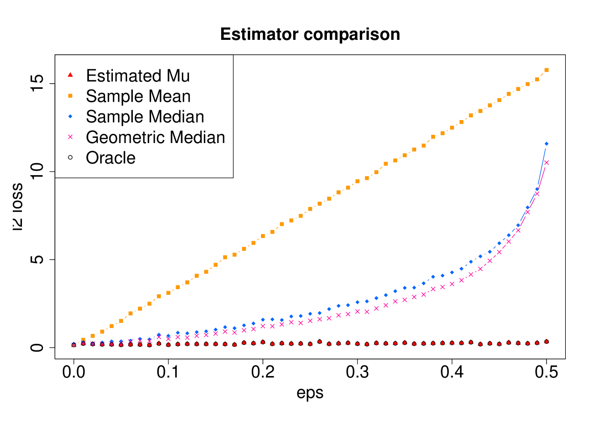
Figure 4: $\ell_{2}$-loss for different estimators when $n=500,p=20$ and the uniform outliers scheme with $a=4$ and $b=10$.

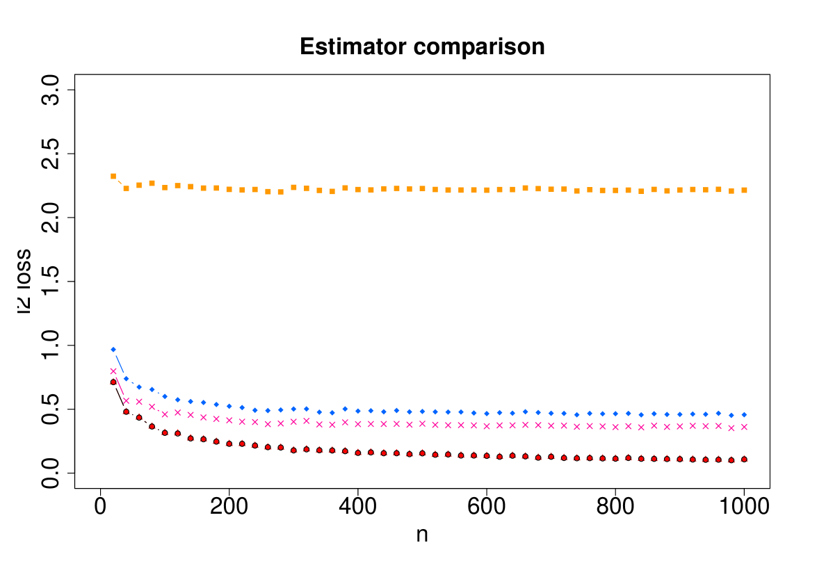
Figure 5: $\ell_{2}$-loss for different estimators when $p=10$, $\varepsilon=0.1$ and the uniform outliers scheme with $a=4$ and $b=10$.

8 Postponed proofs

We collected in this section all the technical proofs postponed from the Section 3 and Section 5. Throughout this section, we will always assume that $\lambda_{\max}(\boldsymbol{\Sigma})=\|\boldsymbol{\Sigma}\|_{\textup{op}}=1$. As we already mentioned above, the general case can be reduced to this one by dividing all the data vectors by $\|\boldsymbol{\Sigma}\|_{\textup{op}}^{1/2}$. The proofs in this section are presented according to the order of the appearance of the corresponding claims in the previous sections. Since the proof of Theorem 5.5 relies on several lemmas and propositions, we provide in Figure 6 a diagram showing the relations between these results.

8.1 Additional details on (23)

One can check that

$$\sum_{i=1}^{n}w_{i}^{*}(\boldsymbol{X}_{i}-\widehat{\boldsymbol{\mu}}^{k-1})^{\otimes 2} =\sum_{i=1}^{n}w_{i}^{*}(\boldsymbol{X}_{i}-\bar{\boldsymbol{X}}_{\boldsymbol{w}^{*}})^{\otimes 2}+(\bar{\boldsymbol{X}}_{\boldsymbol{w}^{*}}-\widehat{\boldsymbol{\mu}}^{k-1})^{\otimes 2}$$ (57)

$$\preceq\sum_{i=1}^{n}w_{i}^{*}(\boldsymbol{X}_{i}-\bar{\boldsymbol{X}}_{\boldsymbol{w}^{*}})^{\otimes 2}+\big{\|}\bar{\boldsymbol{X}}_{\boldsymbol{w}^{*}}-\widehat{\boldsymbol{\mu}}^{k-1}\big{\|}_{2}^{2}\,\mathbf{I}_{p}$$ (58)

$$\preceq\sum_{i=1}^{n}w_{i}^{*}(\boldsymbol{X}_{i}-\boldsymbol{\mu}^{*})^{\otimes 2}+\big{\|}\bar{\boldsymbol{X}}_{\boldsymbol{w}^{*}}-\widehat{\boldsymbol{\mu}}^{k-1}\big{\|}_{2}^{2}\,\mathbf{I}_{p}.$$ (59)

This readily yields

$$G(\boldsymbol{w}^{*},\widehat{\boldsymbol{\mu}}^{k-1}) \leq\lambda_{\max,+}\bigg{(}\sum_{i=1}^{n}w_{i}^{*}(\boldsymbol{X}_{i}-\boldsymbol{\mu}^{*})^{\otimes 2}-\boldsymbol{\Sigma}\bigg{)}+\big{\|}\bar{\boldsymbol{X}}_{\boldsymbol{w}^{*}}-\widehat{\boldsymbol{\mu}}^{k-1}\big{\|}_{2}^{2}$$ (60)

$$\leq G(\boldsymbol{w}^{*},\boldsymbol{\mu}^{*})+\big{(}\big{\|}\bar{\boldsymbol{\zeta}}_{\boldsymbol{w}^{*}}\big{\|}_{2}+\big{\|}\boldsymbol{\mu}^{*}-\widehat{\boldsymbol{\mu}}^{k-1}\big{\|}_{2}\big{)}^{2}.$$ (61)

To get the last line of (23), it suffices to apply the elementary consequence of the Minkowskii inequality $\sqrt{a+(b+c)^{2}}\leq\sqrt{a+b^{2}}+c$, for every $a,b,c>0$.

8.2 Rough bound on the error of the geometric median

This subsection is devoted to the proof of an error estimate of the geometric median. This estimate is rather crude, in terms of its dependence on the sample size, but it is sufficient for our purposes. As a matter of fact, it also shows that the breakdown point of the geometric median is equal to $1/2$.

Lemma 8.11.

For every $\varepsilon\leq 1/2$, the geometric median satisfies the inequality

$$\|\widehat{\boldsymbol{\mu}}_{n}^{\textup{GM}}-\boldsymbol{\mu}^{*}\|_{2} \leq\frac{2}{n(1-2\varepsilon)}\sum_{i=1}^{n}\|\boldsymbol{\zeta}_{i}\|_{2}.$$ (62)

Furthermore, its expected error satisfies

$$\|\widehat{\boldsymbol{\mu}}_{n}^{\textup{GM}}-\boldsymbol{\mu}^{*}\|_{\mathbb{L}_{2}} \leq\frac{2\textbf{{r}}_{\scriptscriptstyle\boldsymbol{\Sigma}}^{1/2}}{1-2\varepsilon}.$$ (63)

Proof 8.12.

Recall that the geometric median of $\boldsymbol{X}_{1},\ldots,\boldsymbol{X}_{n}$ is defined by

$$\widehat{\boldsymbol{\mu}}_{n}^{\textup{GM}}\in\textup{arg}\min_{\boldsymbol{\mu}\in\mathbb{R}^{p}}\sum_{i=1}^{n}\|\boldsymbol{X}_{i}-\boldsymbol{\mu}\|_{2}.$$ (64)

It is clear that

$$\sum_{i=1}^{n}\|\boldsymbol{X}_{i}-\widehat{\boldsymbol{\mu}}_{n}^{\textup{GM}}\|_{2} \leq\sum_{i=1}^{n}\|\boldsymbol{X}_{i}-\boldsymbol{\mu}^{*}\|_{2}$$ (65)

Without loss of generality, we assume that $\boldsymbol{\mu}^{*}=\mathbf{0}$. We also assume that $n\varepsilon$ is an integer. On the one hand, we have the simple bound

$$n(1-\varepsilon)\|\widehat{\boldsymbol{\mu}}_{n}^{\textup{GM}}\|_{2} \leq\sum_{i\in\mathcal{I}}\big{(}\|\boldsymbol{X}_{i}-\widehat{\boldsymbol{\mu}}_{n}^{\textup{GM}}\|_{2}+\|\boldsymbol{\zeta}_{i}\|_{2}\big{)}$$ (66)

$$\leq\sum_{i=1}^{n}\|\boldsymbol{X}_{i}-\widehat{\boldsymbol{\mu}}_{n}^{\textup{GM}}\|_{2}+\sum_{i\in\mathcal{I}}\|\boldsymbol{\zeta}_{i}\|_{2}-\sum_{i\in\mathcal{O}}\|\boldsymbol{X}_{i}-\widehat{\boldsymbol{\mu}}_{n}^{\textup{GM}}\|_{2}$$ (67)

$$\leq\sum_{i=1}^{n}\|\boldsymbol{X}_{i}-\boldsymbol{\mu}^{*}\|_{2}+\sum_{i\in\mathcal{I}}\|\boldsymbol{\zeta}_{i}\|_{2}-\sum_{i\in\mathcal{O}}\|\boldsymbol{X}_{i}-\widehat{\boldsymbol{\mu}}_{n}^{\textup{GM}}\|_{2}$$ (68)

$$\leq 2\sum_{i\in\mathcal{I}}\|\boldsymbol{\zeta}_{i}\|_{2}+\sum_{i\in\mathcal{O}}\big{(}\|\boldsymbol{X}_{i}\|_{2}-\|\boldsymbol{X}_{i}-\widehat{\boldsymbol{\mu}}_{n}^{\textup{GM}}\|_{2}\big{)}$$ (69)

$$\leq 2\sum_{i\in\mathcal{I}}\|\boldsymbol{\zeta}_{i}\|_{2}+n\varepsilon\|\widehat{\boldsymbol{\mu}}_{n}^{\textup{GM}}\|_{2},$$ (70)

where the first and the last inequalities follow from triangle inequality. From the last display, we infer that

$$\|\widehat{\boldsymbol{\mu}}_{n}^{\textup{GM}}\|_{\mathbb{L}_{2}} \leq\frac{2}{n(1-2\varepsilon)}\sum_{i=1}^{n}\|\boldsymbol{\zeta}_{i}\|_{\mathbb{L}_{2}}\leq\frac{2}{1-2\varepsilon}\|\boldsymbol{\zeta}_{1}\|_{\mathbb{L}_{2}}\leq\frac{2\textbf{{r}}_{\scriptscriptstyle\boldsymbol{\Sigma}}^{1/2}}{1-2\varepsilon}$$ (71)

and we get the claim of the lemma.

Figure 6: A diagram showing the relation between different lemmas and propositions used in the proof of Theorem 5.5.

8.3 Proof of Proposition 5.2

To ease notation throughout this proof, we write $\bar{\varepsilon}$ instead of $\varepsilon_{w}$. Simple algebra yields

$$\bar{\boldsymbol{X}}_{\boldsymbol{w}}-\boldsymbol{\mu}^{*}-\bar{\boldsymbol{\zeta}}_{\boldsymbol{w}_{\mathcal{I}}} =\bar{\boldsymbol{X}}_{\boldsymbol{w}_{\mathcal{I}}}+\bar{\boldsymbol{X}}_{\boldsymbol{w}_{\mathcal{I}^{c}}}-\boldsymbol{\mu}^{*}-\bar{\boldsymbol{\zeta}}_{\boldsymbol{w}_{\mathcal{I}}}$$ (72)

$$=(1-\bar{\varepsilon})\boldsymbol{\mu}^{*}+\bar{\boldsymbol{\zeta}}_{\boldsymbol{w}_{\mathcal{I}}}+\bar{\boldsymbol{X}}_{\boldsymbol{w}_{\mathcal{I}^{c}}}-\boldsymbol{\mu}^{*}-\bar{\boldsymbol{\zeta}}_{\boldsymbol{w}_{\mathcal{I}}}$$ (73)

$$=\bar{\boldsymbol{X}}_{\boldsymbol{w}_{\mathcal{I}^{c}}}-\bar{\varepsilon}\boldsymbol{\mu}^{*}$$ (74)

$$=\bar{\boldsymbol{X}}_{\boldsymbol{w}_{\mathcal{I}^{c}}}-\bar{\varepsilon}\bar{\boldsymbol{X}}_{\boldsymbol{w}}+\bar{\varepsilon}(\bar{\boldsymbol{X}}_{\boldsymbol{w}}-\boldsymbol{\mu}^{*}).$$ (75)

This implies that $(1-\bar{\varepsilon})(\bar{\boldsymbol{X}}_{\boldsymbol{w}}-\boldsymbol{\mu}^{*})-\bar{\boldsymbol{\zeta}}_{\boldsymbol{w}_{\mathcal{I}}}=\bar{\boldsymbol{X}}_{\boldsymbol{w}_{\mathcal{I}^{c}}}-\bar{\varepsilon}\bar{\boldsymbol{X}}_{\boldsymbol{w}}$, which is equivalent to

$$\bar{\boldsymbol{X}}_{\boldsymbol{w}}-\boldsymbol{\mu}^{*}-\bar{\boldsymbol{\zeta}}_{\boldsymbol{w}_{|\mathcal{I}}}=\frac{\bar{\boldsymbol{X}}_{\boldsymbol{w}_{\mathcal{I}^{c}}}-\bar{\varepsilon}\bar{\boldsymbol{X}}_{\boldsymbol{w}}}{1-\bar{\varepsilon}}.$$ (76)

Therefore, we have

$$\big{\|}\bar{\boldsymbol{X}}_{\boldsymbol{w}}-\boldsymbol{\mu}^{*}-\bar{\boldsymbol{\zeta}}_{\boldsymbol{w}_{|\mathcal{I}}}\big{\|}_{2} =\frac{\big{\|}\bar{\boldsymbol{X}}_{\boldsymbol{w}_{\mathcal{I}^{c}}}-\bar{\varepsilon}\bar{\boldsymbol{X}}_{\boldsymbol{w}}\big{\|}_{2}}{1-\bar{\varepsilon}}$$ (77)

$$=\frac{1}{1-\bar{\varepsilon}}\bigg{\|}\sum_{i\in\mathcal{I}^{c}}w_{i}(\boldsymbol{X}_{i}-\bar{\boldsymbol{X}}_{\boldsymbol{w}})\bigg{\|}_{2}$$ (78)

$$=\frac{1}{1-\bar{\varepsilon}}\sup_{\boldsymbol{v}\in\mathbb{S}^{p-1}}\sum_{i\in\mathcal{I}^{c}}w_{i}\,\boldsymbol{v}^{\top}(\boldsymbol{X}_{i}-\bar{\boldsymbol{X}}_{\boldsymbol{w}}).$$ (79)

Using the Cauchy-Schwarz inequality as well as the notations $\mathbf{M}_{i}=(\boldsymbol{X}_{i}-\bar{\boldsymbol{X}}_{\boldsymbol{w}})^{\otimes 2}$ and $\mathbf{M}=\sum_{i=1}^{n}w_{i}\mathbf{M}_{i}$, we get

$$\bigg{\{}\sum_{i\in\mathcal{I}^{c}}w_{i}\,\boldsymbol{v}^{\top}(\boldsymbol{X}_{i}-\bar{\boldsymbol{X}}_{\boldsymbol{w}})\bigg{\}}^{2} \leq\sum_{i\in\mathcal{I}^{c}}w_{i}\sum_{i\in\mathcal{I}^{c}}w_{i}|\boldsymbol{v}^{\top}(\boldsymbol{X}_{i}-\bar{\boldsymbol{X}}_{\boldsymbol{w}})|^{2}=\bar{\varepsilon}\,\boldsymbol{v}^{\top}\sum_{i\in\mathcal{I}^{c}}w_{i}\mathbf{M}_{i}\boldsymbol{v}$$ (80)

$$=\bar{\varepsilon}\,\boldsymbol{v}^{\top}\sum_{i=1}^{n}w_{i}\mathbf{M}_{i}\boldsymbol{v}-\boldsymbol{v}^{\top}\sum_{i\in\mathcal{I}}w_{i}\mathbf{M}_{i}\boldsymbol{v}$$ (81)

$$={\bar{\varepsilon}}\,\boldsymbol{v}^{\top}\big{(}\mathbf{M}-\boldsymbol{\Sigma}\big{)}\boldsymbol{v}+{\bar{\varepsilon}}\boldsymbol{v}^{\top}\Big{(}\boldsymbol{\Sigma}-\sum_{i\in\mathcal{I}}w_{i}\mathbf{M}_{i}\Big{)}\boldsymbol{v}$$ (82)

$$\leq\bar{\varepsilon}\,\lambda_{\max}\big{(}\mathbf{M}-\boldsymbol{\Sigma}\big{)}+\bar{\varepsilon}\,\Big{\{}\boldsymbol{v}^{\top}\boldsymbol{\Sigma}\boldsymbol{v}-\boldsymbol{v}^{\top}\sum_{i\in\mathcal{I}}w_{i}\mathbf{M}_{i}\boldsymbol{v}\Big{\}}.$$ (83)

Finally, for any unit vector $\boldsymbol{v}$,

$$\boldsymbol{v}^{\top}\sum_{i\in\mathcal{I}}w_{i}\mathbf{M}_{i}\boldsymbol{v} =(1-\bar{\varepsilon})\,\boldsymbol{v}^{\top}\sum_{i\in\mathcal{I}}(\boldsymbol{w}_{|\mathcal{I}})_{i}(\boldsymbol{X}_{i}-\bar{\boldsymbol{X}}_{\boldsymbol{w}})^{\otimes 2}\boldsymbol{v}$$ (84)

$$\geq(1-\bar{\varepsilon})\,\boldsymbol{v}^{\top}\sum_{i\in\mathcal{I}}(\boldsymbol{w}_{|\mathcal{I}})_{i}(\boldsymbol{X}_{i}-\bar{\boldsymbol{X}}_{\boldsymbol{w}_{|\mathcal{I}}})^{\otimes 2}\boldsymbol{v}$$ (85)

$$=(1-\bar{\varepsilon})\,\boldsymbol{v}^{\top}\sum_{i\in\mathcal{I}}(\boldsymbol{w}_{|\mathcal{I}})_{i}(\boldsymbol{\zeta}_{i}-\bar{\boldsymbol{\zeta}}_{\boldsymbol{w}_{|\mathcal{I}}})^{\otimes 2}\boldsymbol{v}$$ (86)

$$=(1-\bar{\varepsilon})\,\boldsymbol{v}^{\top}\sum_{i\in\mathcal{I}}(\boldsymbol{w}_{|\mathcal{I}})_{i}\boldsymbol{\zeta}_{i}\boldsymbol{\zeta}_{i}^{\top}\boldsymbol{v}-(1-\bar{\varepsilon})\,(\boldsymbol{v}^{\top}\bar{\boldsymbol{\zeta}}_{\boldsymbol{w}_{|\mathcal{I}}})^{2}$$ (87)

$$\geq(1-\bar{\varepsilon})\bigg{(}\boldsymbol{v}^{\top}\boldsymbol{\Sigma}\boldsymbol{v}-\lambda_{\max}\bigg{(}\sum_{i\in\mathcal{I}}(\boldsymbol{w}_{|\mathcal{I}})_{i}(\boldsymbol{\Sigma}-\boldsymbol{\zeta}_{i}\boldsymbol{\zeta}_{i}^{\top})\bigg{)}-\|\bar{\boldsymbol{\zeta}}_{\boldsymbol{w}_{|\mathcal{I}}}\|_{2}^{2}\bigg{)}.$$ (88)

Combining (83) and (88), we get

$$\bigg{\{}\sum_{i\in\mathcal{I}^{c}}w_{i}\,\boldsymbol{v}^{\top}(\boldsymbol{X}_{i}-\boldsymbol{\mu})\bigg{\}}^{2} \leq\bar{\varepsilon}\,\lambda_{\max}\big{(}\mathbf{M}-\boldsymbol{\Sigma}\big{)}+\bar{\varepsilon}^{2}\,\lambda_{\max}\big{(}\boldsymbol{\Sigma}\big{)}$$ (89)

$$\qquad+\bar{\varepsilon}(1-\bar{\varepsilon})\bigg{\{}\lambda_{\max}\bigg{(}\sum_{i\in\mathcal{I}}(\boldsymbol{w}_{|\mathcal{I}})_{i}(\boldsymbol{\Sigma}-\boldsymbol{\zeta}_{i}\boldsymbol{\zeta}_{i}^{\top})\bigg{)}+\|\bar{\boldsymbol{\zeta}}_{\boldsymbol{w}_{|\mathcal{I}}}\|_{2}^{2}\bigg{\}}.$$ (90)

In conjunction with (79), this yields

$$\big{\|}\bar{\boldsymbol{X}}_{\boldsymbol{w}}-\boldsymbol{\mu}^{*}-\bar{\boldsymbol{\zeta}}_{\boldsymbol{w}_{|\mathcal{I}}}\big{\|}_{2} \leq\frac{\sqrt{\bar{\varepsilon}}}{1-\bar{\varepsilon}}\bigg{(}\lambda_{\max}\big{(}\mathbf{M}-\boldsymbol{\Sigma}\big{)}+\bar{\varepsilon}\,\lambda_{\max}\big{(}\boldsymbol{\Sigma}\big{)}$$ (91)

$$\qquad+(1-\bar{\varepsilon})\bigg{\{}\lambda_{\max}\bigg{(}\sum_{i\in\mathcal{I}}(\boldsymbol{w}_{|\mathcal{I}})_{i}(\boldsymbol{\Sigma}-\boldsymbol{\zeta}_{i}\boldsymbol{\zeta}_{i}^{\top})\bigg{)}+\|\bar{\boldsymbol{\zeta}}_{\boldsymbol{w}_{|\mathcal{I}}}\|_{2}^{2}\bigg{\}}\bigg{)}^{1/2}.$$ (92)

From this relation, using the triangle inequality and the inequality $\sqrt{a_{1}+\ldots+a_{n}}\leq\sqrt{a_{1}}+\ldots+\sqrt{a_{n}}$, we get

$$\big{\|}\bar{\boldsymbol{X}}_{\boldsymbol{w}}-\boldsymbol{\mu}^{*}\|_{2} \leq\|\bar{\boldsymbol{\zeta}}_{\boldsymbol{w}_{|\mathcal{I}}}\big{\|}_{2}+\frac{\sqrt{\bar{\varepsilon}}}{1-\bar{\varepsilon}}\lambda_{\max,+}^{1/2}\big{(}\mathbf{M}-\boldsymbol{\Sigma}\big{)}+\frac{{\bar{\varepsilon}}\|\boldsymbol{\Sigma}\|_{\textup{op}}^{1/2}}{1-\bar{\varepsilon}}$$ (93)

$$\qquad+\sqrt{\frac{\bar{\varepsilon}}{1-\bar{\varepsilon}}}\lambda_{\max,+}^{1/2}\bigg{(}\sum_{i\in\mathcal{I}}(\boldsymbol{w}_{|\mathcal{I}})_{i}(\boldsymbol{\Sigma}-\boldsymbol{\zeta}_{i}\boldsymbol{\zeta}_{i}^{\top})\bigg{)}+\sqrt{\frac{\bar{\varepsilon}}{1-\bar{\varepsilon}}}\|\bar{\boldsymbol{\zeta}}_{\boldsymbol{w}_{|\mathcal{I}}}\|_{2}$$ (94)

and, after rearranging the terms, the claim of the proposition follows.

8.4 Proof of Lemma 5.3

Claim i) of this lemma is straightforward. For ii), we use the fact that the compact convex polytope $\mathcal{W}_{n,\ell}$ is the convex hull of its extreme points. The fact that each uniform weight vector $\boldsymbol{u}^{J}$ is an extreme point of $\mathcal{W}_{n,\ell}$ is easy to check. Indeed, if for two points $\boldsymbol{w}$ and $\boldsymbol{w}^{\prime}$ from $\mathcal{W}_{n,\ell}$ we have $\boldsymbol{u}^{J}=0.5(\boldsymbol{w}+\boldsymbol{w}^{\prime})$, then we necessarily have $\boldsymbol{w}_{J^{c}}=\boldsymbol{w}^{\prime}_{J^{c}}=0$. Therefore, for any $j\in J$,

$$\frac{1}{\ell}\geq w_{j}=1-\sum_{i\in J\setminus\{j\}}w_{i}\geq 1-\big{(}\ell-1)\times\frac{1}{\ell}=\frac{1}{\ell}.$$ (95)

This implies that $w_{j}=\frac{1}{\ell}\mathds{1}(j\in J)$. Hence, $\boldsymbol{w}=\boldsymbol{u}^{J}$ and the same is true for $\boldsymbol{w}^{\prime}$. Hence, $\boldsymbol{u}^{J}$ is an extreme point. Let us prove now that all the extreme points of $\mathcal{W}_{n,\ell}$ are of the form $\boldsymbol{u}^{J}$ with $|J|=\ell$. Let $\boldsymbol{w}\in\mathcal{W}_{n,\ell}$ be such that one of its coordinates is strictly positive and strictly smaller than $1/\ell$. Without loss of generality, we assume that the two smallest nonzero entries of $\boldsymbol{w}$ are $w_{1}$ and $w_{2}$. We have $0<w_{1}<1/\ell$ and $0<w_{2}<1/\ell$. Set $\rho=w_{1}\wedge w_{2}\wedge\{1/\ell-w_{1}\}\wedge\{1/\ell-w_{2}\}$. For $\boldsymbol{w}^{+}=\boldsymbol{w}+(\rho,-\rho,0,\ldots,0)$ and $\boldsymbol{w}^{-}=\boldsymbol{w}-(\rho,-\rho,0,\ldots,0)$, we have $\boldsymbol{w}^{+},\boldsymbol{w}^{-}\in\mathcal{W}_{n,\ell}$ and $\boldsymbol{w}=0.5(\boldsymbol{w}^{+}+\boldsymbol{w}^{-})$. Therefore, $\boldsymbol{w}$ is not an extreme point of $\mathcal{W}_{n,\ell}$. This completes the proof of ii).

Claim ii) implies that $\mathcal{W}_{n,\ell}=\{\sum_{|J|=\ell}\alpha_{J}\boldsymbol{u}^{J}:\boldsymbol{\alpha}\in\boldsymbol{\Delta}^{K-1}\}$ with $K={n\choose\ell}$. Hence,

$$\sup_{\boldsymbol{w}\in\mathcal{W}_{n,\ell}}G(\boldsymbol{w}) =\sup_{\boldsymbol{\alpha}\in\boldsymbol{\Delta}^{K-1}}G\bigg{(}\sum_{|J|=\ell}\alpha_{J}\boldsymbol{u}^{J}\bigg{)}\leq\sup_{\boldsymbol{\alpha}\in\boldsymbol{\Delta}^{K-1}}\sum_{|J|=\ell}\alpha_{J}G\big{(}\boldsymbol{u}^{J}\big{)}\leq\max_{|J|=\ell}G(\boldsymbol{u}^{J})$$ (96)

and claim iii) follows.

To prove iv), we check that

$$\|\boldsymbol{w}_{I}\|_{1}=\sum_{i\in I}w_{i}=1-\sum_{i\not\in I}w_{i}\geq 1-\frac{|I^{c}|}{\ell}\geq 1-\frac{n-\ell^{\prime}}{\ell}=\frac{\ell+\ell^{\prime}-n}{\ell}.$$ (97)

This readily yields $(\boldsymbol{w}_{|I})_{i}\leq 1/(\ell+\ell^{\prime}-n)$, which leads to the claim of item iv).

8.5 Moments of suprema over $\mathcal{W}_{n,\ell}$ of weighted averages of Gaussian vectors

We recall that $\boldsymbol{\xi}_{i}$’s, for $i=1,\ldots,n$ are i.i.d. Gaussian vectors with zero mean and identity covariance matrix, and $\boldsymbol{\zeta}_{i}=\boldsymbol{\Sigma}^{1/2}\boldsymbol{\xi}_{i}$. In addition, the covariance matrix $\boldsymbol{\Sigma}$ satisfies $\|\boldsymbol{\Sigma}\|_{\textup{op}}=1$.

Lemma 8.13.

Let $p\geq 1$, $n\geq 1$, $m\in[2,0.562n]$ and $o\in[0,m]$ be four positive integers. It holds that

$$\mathbf{E}^{1/2}\Bigg{[}\sup_{\begin{subarray}{c}\boldsymbol{w}\in\mathcal{W}_{n,n-m+o}\\ |I|\geq n-o\end{subarray}}{\|\bar{\boldsymbol{\zeta}}_{\boldsymbol{w}_{|I}}\|}_{2}^{2}\Bigg{]}\leq{\sqrt{\textbf{{r}}_{\scriptscriptstyle\boldsymbol{\Sigma}}/n}}\,\bigg{(}1+7\sqrt{\frac{m}{2n}}\bigg{)}+\frac{4.6m}{n}\sqrt{\log(\nicefrac{{ne}}{{m}})}.$$ (98)

Proof 8.14 (Proof of Lemma 8.13).

We have

$$\sup_{\boldsymbol{w}\in\mathcal{W}_{n,n-m+o}}\|\bar{\boldsymbol{\zeta}}_{\boldsymbol{w}_{|I}}\|_{2} \stackrel{{\scriptstyle(a)}}{{\leq}}\sup_{\boldsymbol{w}\in\mathcal{W}_{n,n-m}}\|\bar{\boldsymbol{\zeta}}_{\boldsymbol{w}}\|_{2}\stackrel{{\scriptstyle(b)}}{{\leq}}\max_{|J|=n-m}\big{\|}\bar{\boldsymbol{\zeta}}_{\boldsymbol{u}^{J}}\big{\|}_{2},$$ (99)

where $(a)$ follows from claim iv) of Lemma 5.3 and $(b)$ is a direct consequence of claim iii) of Lemma 5.3. Thus, we get

$$\sup_{\boldsymbol{w}\in\mathcal{W}_{n,n-m+o}}\|\bar{\boldsymbol{\zeta}}_{\boldsymbol{w}_{|I}}\|_{2} \leq\max_{|J|=n-m}{\big{\|}\bar{\boldsymbol{\zeta}}_{\boldsymbol{u}^{J}}\big{\|}}_{2}=\frac{1}{n-m}\max_{|J|=n-m}\bigg{\|}\sum_{i\in J}\boldsymbol{\zeta}_{i}\bigg{\|}_{2}$$ (100)

$$\leq\frac{1}{n-m}\bigg{\|}\sum_{i=1}^{n}\boldsymbol{\zeta}_{i}\bigg{\|}_{2}+\frac{1}{n-m}\max_{|\bar{J}|=m}\bigg{\|}\sum_{i\in\bar{J}}\boldsymbol{\zeta}_{i}\bigg{\|}_{2}.$$ (101)

On the one hand, one readily checks that

$$\mathbf{E}\bigg{[}\bigg{\|}\sum_{i=1}^{n}\boldsymbol{\zeta}_{i}\bigg{\|}_{2}^{2}\bigg{]}=n\textbf{{r}}_{\scriptscriptstyle\boldsymbol{\Sigma}}.$$ (102)

On the other hand, it is clear that for every $\bar{J}$ of cardinality $m$, the random variable $\big{\|}\sum_{i\in\bar{J}}\boldsymbol{\zeta}_{i}\big{\|}^{2}_{2}$ has the same distribution as $m\sum_{j=1}^{p}\lambda_{j}(\boldsymbol{\Sigma})\xi_{j}^{2}$, where $\xi_{1},\ldots,\xi_{p}$ are i.i.d. standard Gaussian. Therefore, by the union bound, for every $t\geq 0$, we have

$$\mathbf{P}\bigg{(}\max_{|\bar{J}|=m}\bigg{\|}\sum_{i\in\bar{J}}\boldsymbol{\zeta}_{i}\bigg{\|}^{2}_{2}>m\big{(}2\textbf{{r}}_{\scriptscriptstyle\boldsymbol{\Sigma}}+t\big{)}\bigg{)} \leq{{n}\choose{m}}\mathbf{P}\bigg{(}\bigg{\|}\sum_{i=1}^{m}\boldsymbol{\zeta}_{i}\bigg{\|}_{2}^{2}>m\big{(}2\textbf{{r}}_{\scriptscriptstyle\boldsymbol{\Sigma}}+t\big{)}\bigg{)}$$ (103)

$$={{n}\choose{m}}\mathbf{P}\bigg{(}\sum_{j=1}^{p}\lambda_{j}(\boldsymbol{\Sigma})\xi_{j}^{2}>2\textbf{{r}}_{\scriptscriptstyle\boldsymbol{\Sigma}}+t\bigg{)}\leq{{n}\choose{m}}e^{-t/3},$$ (104)

where the last line follows from a well-known bound on the tails of the generalized $\chi^{2}$-distribution, see for instance [Comminges and Dalalyan, 2012, Lemma 8].

Therefore, setting $Z=\frac{1}{m}\max_{|J|=m}\big{\|}\sum_{i\in J}\boldsymbol{\zeta}_{i}\big{\|}^{2}_{2}-2\textbf{{r}}_{\scriptscriptstyle\boldsymbol{\Sigma}}$ and using the well-known identity $\mathbf{E}[Z]\leq\mathbf{E}[Z_{+}]=\int_{0}^{\infty}\mathbf{P}(Z\geq t)\,dt$, we get

$$\mathbf{E}\bigg{[}\max_{|\bar{J}|=m}\frac{1}{m}\bigg{\|}\sum_{i\in\bar{J}}\boldsymbol{\zeta}_{i}\bigg{\|}^{2}_{2}\bigg{]} \leq 2\textbf{{r}}_{\scriptscriptstyle\boldsymbol{\Sigma}}+\int_{0}^{\infty}1\wedge{{n}\choose{m}}e^{-t/3}\,dt$$ (105)

$$=2\textbf{{r}}_{\scriptscriptstyle\boldsymbol{\Sigma}}+3\log{{n}\choose{m}}+{{n}\choose{m}}\int_{3\log{{n}\choose{m}}}^{\infty}e^{-t/3}\,dt$$ (106)

$$\leq 2\textbf{{r}}_{\scriptscriptstyle\boldsymbol{\Sigma}}+3m\log(\nicefrac{{ne}}{{m}})+3$$ (107)

$$\leq 2\textbf{{r}}_{\scriptscriptstyle\boldsymbol{\Sigma}}+3.9m\log(\nicefrac{{ne}}{{m}}),$$ (108)

where the last two steps follow from the inequality $\log{n\choose{m}}\leq m\log(ne/m)$ and the fact that $m\geq 2$, $m\log(\nicefrac{{ne}}{{m}})\geq n\inf_{x\in[2/n,1]}x(1-\log x)\geq 2(1-\log(2/n))\geq 10/3$. Combining (101), (102) and (108), we arrive at

$$\bigg{(}\mathbf{E}\bigg{[}\sup_{\begin{subarray}{c}\boldsymbol{w}\in\mathcal{W}_{n,n-m+o}\\ |I|\geq n-o\end{subarray}}{\|\bar{\boldsymbol{\zeta}}_{\boldsymbol{w}_{|I}}\|}_{2}^{2}\bigg{]}\bigg{)}^{1/2} \leq\frac{\sqrt{n\textbf{{r}}_{\scriptscriptstyle\boldsymbol{\Sigma}}}}{n-m}+\frac{\sqrt{m}}{n-m}\times\big{(}2\textbf{{r}}_{\scriptscriptstyle\boldsymbol{\Sigma}}+3.9m\log(\nicefrac{{ne}}{{m}})\big{)}^{1/2}$$ (109)

$$\leq\sqrt{\textbf{{r}}_{\scriptscriptstyle\boldsymbol{\Sigma}}/n}\Big{(}1+\frac{m}{n-m}+\frac{\sqrt{2mn}}{n-m}\Big{)}+\frac{4.6m}{n}\sqrt{\log(\nicefrac{{ne}}{{m}})}.$$ (110)

Finally, note that for $\alpha=m/n\leq 0.562$, we have

$$\frac{m}{n-m}+\frac{\sqrt{2mn}}{n-m} =\sqrt{\frac{m}{2n}}\bigg{(}\frac{\sqrt{2mn}}{n-m}+\frac{2n}{n-m}\bigg{)}$$ (111)

$$=\sqrt{\frac{m}{2n}}\bigg{(}\frac{\sqrt{2\alpha}}{1-\alpha}+\frac{2}{1-\alpha}\bigg{)}\leq 7\sqrt{\frac{m}{2n}}.$$ (112)

This completes the proof of the lemma.

8.6 Moments and deviations of singular values of Gaussian matrices

Let $\boldsymbol{\zeta}_{1},\ldots,\boldsymbol{\zeta}_{n}$ be i.i.d. random vectors drawn from $\mathcal{N}_{p}(0,\boldsymbol{\Sigma})$ distribution, where $\boldsymbol{\Sigma}$ is a $p\times p$ covariance matrix. We denote by $\boldsymbol{\zeta}_{1:n}$ the $p\times n$ random matrix obtained by concatenating the vectors $\boldsymbol{\zeta}_{i}$. Recall that $s_{\min}(\boldsymbol{\zeta}_{1:n})=\lambda_{\min}^{1/2}(\boldsymbol{\zeta}_{1:n}\boldsymbol{\zeta}_{1:n}^{\top})$ and $s_{\max}(\boldsymbol{\zeta}_{1:n})=\lambda_{\max}^{1/2}(\boldsymbol{\zeta}_{1:n}\boldsymbol{\zeta}_{1:n}^{\top})$ are the smallest and the largest singular values of the matrix $\boldsymbol{\zeta}_{1:n}$.

Lemma 8.15 (Vershynin [2012], Theorem 5.32 and Corollary 5.35).

Let $\lambda_{\max}(\boldsymbol{\Sigma})=1$. For every $t>0$ and for every pair of positive integers $n$ and $p$, we have

$$\mathbf{E}\big{[}s_{\max}(\boldsymbol{\zeta}_{1:n})\big{]} \leq\sqrt{n}+\sqrt{\textbf{{r}}_{\scriptscriptstyle\boldsymbol{\Sigma}}},\quad \mathbf{P}\big{(}s_{\max}(\boldsymbol{\zeta}_{1:n})\geq\sqrt{n}+\sqrt{\textbf{{r}}_{\scriptscriptstyle\boldsymbol{\Sigma}}}+t\big{)}\leq e^{-t^{2}/2}.$$ (113)

If, in addition, $\boldsymbol{\Sigma}$ is the identity matrix, then

$$\mathbf{E}\big{[}s_{\min}(\boldsymbol{\zeta}_{1:n})\big{]} \geq{\big{(}\sqrt{n}-\sqrt{p}\big{)}}_{+},\quad \mathbf{P}\big{(}s_{\min}(\boldsymbol{\zeta}_{1:n})\leq\sqrt{n}-\sqrt{p}-t\big{)}\leq e^{-t^{2}/2}.$$ (114)

The corresponding results in [Vershynin, 2012] treat only the case of identity covariance matrix $\boldsymbol{\Sigma}=\mathbf{I}_{p}$, however the proof presented therein carries with almost no change over the case of arbitrary covariance matrix. These bounds allow us to establish the following inequalities.

Lemma 8.16.

For a subset $\bar{J}$ of $\{1,\ldots,n\}$, we denote by $\boldsymbol{\zeta}_{\bar{J}}$ the $p\times|\bar{J}|$ matrix obtained by concatenating the vectors $\{\boldsymbol{\zeta}_{i}:i\in\bar{J}\}$. Let the covariance matrix $\boldsymbol{\Sigma}$ be such that $\lambda_{\max}(\boldsymbol{\Sigma})=1$. For every pair of integers $n,p\geq 1$ and for every integer $m\in[1,n]$, we have

$$\mathbf{E}\big{[}s_{\max}^{2}(\boldsymbol{\zeta}_{1:n})\big{]} \leq\big{(}\sqrt{\textbf{{r}}_{\scriptscriptstyle\boldsymbol{\Sigma}}}+\sqrt{n}\big{)}^{2}+4,$$ (115)

$$\mathbf{E}\big{[}(s_{\max}(\boldsymbol{\zeta}_{1:n})^{2}-n)_{+}\big{]} \leq 6\sqrt{n\textbf{{r}}_{\scriptscriptstyle\boldsymbol{\Sigma}}}+4\textbf{{r}}_{\scriptscriptstyle\boldsymbol{\Sigma}},\qquad\forall n\geq 8,$$ (116)

$$\mathbf{E}\big{[}(n-s_{\min}(\boldsymbol{\xi}_{1:n})^{2})_{+}\big{]} \leq 6\sqrt{np},\qquad\forall n\geq 8,$$ (117)

$$\mathbf{E}\Big{[}\max_{|\bar{J}|=m}s_{\max}^{2}(\boldsymbol{\zeta}_{\bar{J}})\Big{]} \leq\big{(}\sqrt{\textbf{{r}}_{\scriptscriptstyle\boldsymbol{\Sigma}}}+\sqrt{m}+1.81\sqrt{m\log(\nicefrac{{ne}}{{m}})}\big{)}^{2}+4.$$ (118)

Proof 8.17.

The bias-variance decomposition, in conjunction with Lemma 8.15, yields

$$\mathbf{E}\big{[}s_{\max}^{2}(\boldsymbol{\zeta}_{1:n})\big{]} =\textbf{Var}\big{(}s_{\max}(\boldsymbol{\zeta}_{1:n})\big{)}+\mathbf{E}\big{[}s_{\max}(\boldsymbol{\zeta}_{1:n})\big{]}^{2}$$ (119)

$$\leq\textbf{Var}\big{(}s_{\max}(\boldsymbol{\zeta}_{1:n})\big{)}+\big{(}\sqrt{n}+\sqrt{\textbf{{r}}_{\scriptscriptstyle\boldsymbol{\Sigma}}}\big{)}^{2}.$$ (120)

Applying the well-known fact $\mathbf{E}[Z^{2}]=\int_{0}^{\infty}\mathbf{P}(Z^{2}\geq t)\,dt$ to the random variable $Z=s_{\max}(\boldsymbol{\zeta}_{1:n})-\mathbf{E}[s_{\max}(\boldsymbol{\zeta}_{1:n})]$ and using the Gaussian concentration inequality, we get

$$\textbf{Var}\big{(}s_{\max}(\boldsymbol{\zeta}_{1:n})\big{)} =\int_{0}^{\infty}\mathbf{P}\Big{(}\big{|}s_{\max}(\boldsymbol{\zeta}_{1:n})-\mathbf{E}[s_{\max}(\boldsymbol{\zeta}_{1:n})]\big{|}\geq\sqrt{t}\Big{)}\,dt\leq 2\int_{0}^{\infty}e^{-t/2}\,dt=4.$$ (121)

This completes the proof of (115).

For every random variable $Z$ and every constant $a>0$, we have

$$\mathbf{E}\big{[}((a+Z)^{2}-n)_{+}\big{]} =\mathbf{E}\big{[}(a^{2}+2aZ+Z^{2}-n)_{+}\big{]}$$ (122)

$$\leq\mathbf{E}\big{[}(a^{2}+2aZ-n)_{+}\big{]}+\mathbf{E}[Z^{2}]$$ (123)

$$\leq|a^{2}-n|+2a\mathbf{E}[Z_{+}]+\mathbf{E}[Z^{2}].$$ (124)

Taking $a=\mathbf{E}[s_{\max}(\boldsymbol{\zeta}_{1:n})]$ and $Z=s_{\max}(\boldsymbol{\zeta}_{1:n})-\mathbf{E}[s_{\max}(\boldsymbol{\zeta}_{1:n})]$, we get

$$\mathbf{E}\big{[}(s_{\max}(\boldsymbol{\zeta}_{1:n})^{2}-n)_{+}\big{]} \leq|(\sqrt{n}+\sqrt{\textbf{{r}}_{\scriptscriptstyle\boldsymbol{\Sigma}}})^{2}-n|+(\sqrt{n}+\sqrt{\textbf{{r}}_{\scriptscriptstyle\boldsymbol{\Sigma}}})\sqrt{2\pi}+4$$ (125)

$$=2\sqrt{n\textbf{{r}}_{\scriptscriptstyle\boldsymbol{\Sigma}}}+\textbf{{r}}_{\scriptscriptstyle\boldsymbol{\Sigma}}+(\sqrt{n}+\sqrt{\textbf{{r}}_{\scriptscriptstyle\boldsymbol{\Sigma}}})\sqrt{2\pi}+4$$ (126)

$$\leq 6\sqrt{n\textbf{{r}}_{\scriptscriptstyle\boldsymbol{\Sigma}}}+4\textbf{{r}}_{\scriptscriptstyle\boldsymbol{\Sigma}},\qquad\forall n\geq 8.$$ (127)

Similarly, we have

$$\mathbf{E}\big{[}(n-(a+Z)^{2})_{+}\big{]} =\mathbf{E}\big{[}(n-a^{2}-2aZ-Z^{2})_{+}\big{]}\leq(n-a^{2})_{+}+2a\mathbf{E}\big{[}Z_{-}\big{]}.$$ (128)

Taking $a=\mathbf{E}[s_{\min}(\boldsymbol{\xi}_{1:n})]$ and $Z=s_{\min}(\boldsymbol{\xi}_{1:n})-\mathbf{E}[s_{\min}(\boldsymbol{\xi}_{1:n})]$, we get

$$\mathbf{E}\big{[}(n-s_{\min}(\boldsymbol{\xi}_{1:n})^{2})_{+}\big{]} \leq(n-\mathbf{E}[s_{\min}(\boldsymbol{\xi}_{1:n})]^{2})_{+}+\mathbf{E}[s_{\min}(\boldsymbol{\xi}_{1:n})]\sqrt{2\pi}$$ (129)

$$\leq(n-(\sqrt{n}-\sqrt{p})^{2})_{+}+(\sqrt{n}+\sqrt{p})\sqrt{2\pi}$$ (130)

$$\leq 2\sqrt{np}+(\sqrt{n}+\sqrt{p})\sqrt{2\pi}\leq 6\sqrt{np}.$$ (131)

Thus, we have checked (116) and (117).

In view of Lemma 8.15, for every $t>0$,

$$\mathbf{P}\Big{(}s_{\max}\big{(}\boldsymbol{\zeta}_{\bar{J}}\big{)}<\sqrt{|\vbox to7.0pt{\hbox{$\bar{J}$}}|}+\sqrt{\textbf{{r}}_{\scriptscriptstyle\boldsymbol{\Sigma}}}+t\Big{)}\geq 1-e^{-t^{2}/2}.$$ (132)

Let $I_{0}\subset[n]$ be any set of cardinality $m$. Combining the relation $\mathbf{E}[Z]=\int_{0}^{\infty}\mathbf{P}(Z\geq s)\,ds$, the union bound, and (132), we arrive at

$$\mathbf{E}\Big{[}\max_{|\bar{J}|=m}s_{\max}(\boldsymbol{\zeta}_{\bar{J}})\Big{]} \leq\sqrt{m}+\sqrt{\textbf{{r}}_{\scriptscriptstyle\boldsymbol{\Sigma}}}+\mathbf{E}\Big{[}\max_{|\bar{J}|=m}\big{(}s_{\max}(\boldsymbol{\zeta}_{\bar{J}})-\sqrt{m}-\sqrt{\textbf{{r}}_{\scriptscriptstyle\boldsymbol{\Sigma}}}\big{)}_{+}\Big{]}$$ (133)

$$=\sqrt{m}+\sqrt{\textbf{{r}}_{\scriptscriptstyle\boldsymbol{\Sigma}}}+\int_{0}^{\infty}\mathbf{P}\Big{(}\max_{|\bar{J}|=m}s_{\max}(\boldsymbol{\zeta}_{\bar{J}})\geq\sqrt{m}+\sqrt{\textbf{{r}}_{\scriptscriptstyle\boldsymbol{\Sigma}}}+t\Big{)}\,dt$$ (134)

$$\leq\sqrt{m}+\sqrt{\textbf{{r}}_{\scriptscriptstyle\boldsymbol{\Sigma}}}+\int_{0}^{\infty}1\bigwedge{n\choose{m}}\mathbf{P}\Big{(}s_{\max}(\boldsymbol{\zeta}_{I_{0}})\geq\sqrt{m}+\sqrt{\textbf{{r}}_{\scriptscriptstyle\boldsymbol{\Sigma}}}+t\Big{)}\,dt$$ (135)

$$\leq\sqrt{m}+\sqrt{\textbf{{r}}_{\scriptscriptstyle\boldsymbol{\Sigma}}}+\int_{0}^{\infty}\bigg{\{}1\bigwedge{n\choose{m}}e^{-t^{2}/2}\bigg{\}}\,dt.$$ (136)

From now on, we assume that $m\in[2,n-1]$, which implies that ${n\choose{m}}\geq n$. Let $t_{0}$ be the value of $t$ for which the two terms in the last minimum coincide, that is

$${n\choose{m}}e^{-t_{0}^{2}/2}=1\quad \Longleftrightarrow\quad t_{0}^{2}=2\log{n\choose{m}}\quad\Longrightarrow\quad\begin{cases}t_{0}^{2}\leq 2m\log(\nicefrac{{ne}}{{m}}),\\ t_{0}^{2}\geq 2\log(\nicefrac{{n(n-1)}}{{2}}),\end{cases}$$ (137)

We have, for $m\geq 1$,

$$\int_{0}^{\infty}\bigg{\{}1\bigwedge{n\choose{m}}e^{-t^{2}/2}\bigg{\}}\,dt =t_{0}+{n\choose{m}}\int_{t_{0}}^{\infty}e^{-t^{2}/2}\,dt\leq{t_{0}}+{n\choose{m}}\frac{e^{-t^{2}_{0}/2}}{t_{0}}$$ (138)

$$\leq{t_{0}}+\frac{1}{t_{0}}\leq 1.81\sqrt{m\log(\nicefrac{{ne}}{{m}})}.$$ (139)

Inequalities (136) and (139) yield

$$\mathbf{E}\Big{[}\max_{|\bar{J}|=m}s_{\max}\big{(}\boldsymbol{\zeta}_{\bar{J}}\big{)}\Big{]} \leq\sqrt{m}+\sqrt{\textbf{{r}}_{\scriptscriptstyle\boldsymbol{\Sigma}}}+1.81\sqrt{m\log(\nicefrac{{ne}}{{m}})}.$$ (140)

On the other hand, the mapping $\boldsymbol{\zeta}_{1:n}\mapsto F(\boldsymbol{\zeta}_{1:n}):=\max_{|\bar{J}|=m}s_{\max}\big{(}\boldsymbol{\zeta}_{\bar{J}}\big{)}$ being 1-Lipschitz, the Gaussian concentration inequality leads to

$$\textbf{Var}\Big{(}\max_{|\bar{J}|=m}s_{\max}\big{(}\boldsymbol{\zeta}_{\bar{J}}\big{)}\Big{)} =\int_{0}^{\infty}\textbf{P}\Big{(}\big{|}F(\boldsymbol{\zeta}_{1:n})-\mathbf{E}[F(\boldsymbol{\zeta}_{1:n})]\big{|}\geq\sqrt{t}\Big{)}\,dt\leq 2\int_{0}^{\infty}e^{-t/2}\,dt=4.$$ (141)

This completes the proof of the lemma.

Lemma 8.18.

There is a constant $A_{1}>0$ such that for every pair of integers $n\geq 8$ and $p\geq 1$ and for every covariance matrix $\boldsymbol{\Sigma}$ such that $\lambda_{\max}(\boldsymbol{\Sigma})=1$, we have

$$\mathbf{E}\Big{[}\|\boldsymbol{\zeta}_{1:n}\boldsymbol{\zeta}_{1:n}^{\top}-n\boldsymbol{\Sigma}\|_{\textup{op}}\Big{]} \leq A_{1}\big{(}\sqrt{n}+\sqrt{\textbf{{r}}_{\scriptscriptstyle\boldsymbol{\Sigma}}}\big{)}\sqrt{\textbf{{r}}_{\scriptscriptstyle\boldsymbol{\Sigma}}},$$ (142)

$$\mathbf{E}\Big{[}\lambda_{\max,+}(\boldsymbol{\zeta}_{1:n}\boldsymbol{\zeta}_{1:n}^{\top}-n\boldsymbol{\Sigma})\Big{]} \leq 6\sqrt{np}+4p,$$ (143)

$$\mathbf{E}\Big{[}\lambda_{\max,+}(n\boldsymbol{\Sigma}-\boldsymbol{\zeta}_{1:n}\boldsymbol{\zeta}_{1:n}^{\top})\Big{]} \leq 6\sqrt{np},$$ (144)

where the last inequality is valid under the additional assumption $p\leq n$. Furthermore, there is a constant $A_{2}>0$ such that

$$\mathbf{P}\bigg{(}\|\boldsymbol{\zeta}_{1:n}\boldsymbol{\zeta}_{1:n}^{\top}-n\boldsymbol{\Sigma}\|_{\textup{op}}-\mathbf{E}\Big{[}\|\boldsymbol{\zeta}_{1:n}\boldsymbol{\zeta}_{1:n}^{\top}-n\boldsymbol{\Sigma}\|_{\textup{op}}\Big{]}\geq A_{2}\Big{(}\sqrt{tn}+\sqrt{t\textbf{{r}}_{\scriptscriptstyle\boldsymbol{\Sigma}}}+t\Big{)}\bigg{)}\leq e^{-t},\quad\forall t\geq 1.$$ (145)

Proof 8.19.

Inequality (142) and the last claim of the lemma are respectively Theorems 4 and 5 in [Koltchinskii and Lounici, 2017]. Let us prove the two other claims. Since $\boldsymbol{\zeta}_{i}=\boldsymbol{\Sigma}^{1/2}\boldsymbol{\xi}_{i}$ where $\boldsymbol{\xi}_{i}$’s are i.i.d. $\mathcal{N}(0,\mathbf{I}_{p})$, we have

$$\lambda_{\max,+}(\boldsymbol{\zeta}_{1:n}\boldsymbol{\zeta}_{1:n}^{\top}-n\boldsymbol{\Sigma}) \leq\lambda_{\max,+}(\boldsymbol{\xi}_{1:n}\boldsymbol{\xi}_{1:n}^{\top}-n\mathbf{I}_{p})=\big{(}s_{\max}(\boldsymbol{\xi}_{1:n})^{2}-n\big{)}_{+}.$$ (146)

Inequality (143) now follows from (116) applied in the case of an identity covariance matrix so that $\textbf{{r}}_{\scriptscriptstyle\boldsymbol{\Sigma}}=p$. Similarly, (144) follows from (117) using the same argument.

8.7 Moments of suprema over $\mathcal{W}_{n,\ell}$ of weighted centered Wishart matrices

Lemma 8.20.

Let $p\geq 2$, $n\geq 4\vee p$, $m\in[2,0.6n]$ and $o\leq m$ be four integers. It holds that

$$\mathbf{E} \Bigg{[}\sup_{\begin{subarray}{c}\boldsymbol{w}\in\mathcal{W}_{n,n-m+o}\\ |I|\geq n-o\end{subarray}}\lambda_{\max,+}\Big{(}\boldsymbol{\Sigma}-\sum_{i=1}^{n}(\boldsymbol{w}_{|I})_{i}\boldsymbol{\zeta}_{i}\boldsymbol{\zeta}_{i}^{\top}\Big{)}\Bigg{]}\leq 25\sqrt{p/n}+33(m/n)\log({n}/{m}).$$ (147)

Furthermore, for any $p\geq 1$, $n\geq 1$, $m\in[2,0.6n]$ and $o\leq m$,

$$\mathbf{E} \bigg{[}\sup_{\begin{subarray}{c}\boldsymbol{w}\in\mathcal{W}_{n,n-m+o}\\ |I|\geq n-o\end{subarray}}\Big{\|}\boldsymbol{\Sigma}-\sum_{i=1}^{n}(\boldsymbol{w}_{|I})_{i}\boldsymbol{\zeta}_{i}\boldsymbol{\zeta}_{i}^{\top}\Big{\|}_{\textup{op}}\bigg{]}\leq(5.1A_{1}+2.5A_{2})\sqrt{\frac{\textbf{{r}}_{\scriptscriptstyle\boldsymbol{\Sigma}}}{n}}+7.5A_{2}\frac{m\log(\nicefrac{{ne}}{{m}})}{n},$$ (148)

where $A_{1}$ and $A_{2}$ are the same constants as in Lemma 8.18.

Proof 8.21 (Proof of Lemma 8.20).

For every $I\subset[n]$ such that $|I|\geq n-o$, we have

$$\sup_{\boldsymbol{w}\in\mathcal{W}_{n,n-m+o}}\lambda_{\max,+}\Big{(}\boldsymbol{\Sigma}-\sum_{i=1}^{n}(\boldsymbol{w}_{|I})_{i}\boldsymbol{\zeta}_{i}\boldsymbol{\zeta}_{i}^{\top}\Big{)} \stackrel{{\scriptstyle(a)}}{{\leq}}\sup_{\boldsymbol{w}\in\mathcal{W}_{n,n-m}}\lambda_{\max,+}\Big{(}\boldsymbol{\Sigma}-\sum_{i=1}^{n}w_{i}\boldsymbol{\zeta}_{i}\boldsymbol{\zeta}_{i}^{\top}\Big{)}$$ (149)

$$\stackrel{{\scriptstyle(b)}}{{\leq}}\sup_{|J|=n-m}\lambda_{\max,+}\Big{(}\sum_{i=1}^{n}u^{J}_{i}(\boldsymbol{\Sigma}-\boldsymbol{\zeta}_{i}\boldsymbol{\zeta}_{i}^{\top})\Big{)}.$$ (150)

In the above inequalities, $(a)$ follows from claim iv) of Lemma 5.3, while $(b)$ is a direct consequence of Lemma 5.3, claim iii). Thus, we can infer that for every $\boldsymbol{w}\in\mathcal{W}_{n,n-m+o}$,

$$(n-m)\lambda_{\max,+} \Big{(}\boldsymbol{\Sigma}-\sum_{i=1}^{n}(\boldsymbol{w}_{|I})_{i}\boldsymbol{\zeta}_{i}\boldsymbol{\zeta}_{i}^{\top}\Big{)}\leq\max_{|J|=n-m}\lambda_{\max,+}\Big{(}\sum_{i\in J}(\boldsymbol{\Sigma}-\boldsymbol{\zeta}_{i}\boldsymbol{\zeta}_{i}^{\top})\Big{)}$$ (151)

$$\leq\lambda_{\max,+}\bigg{(}\sum_{i=1}^{n}(\boldsymbol{\Sigma}-\boldsymbol{\zeta}_{i}\boldsymbol{\zeta}_{i}^{\top})\bigg{)}+\max_{|\bar{J}|=m}\lambda_{\max,+}\bigg{(}\sum_{i\in\bar{J}}(\boldsymbol{\zeta}_{i}\boldsymbol{\zeta}_{i}^{\top}-\boldsymbol{\Sigma})\bigg{)}$$ (152)

$$\leq\lambda_{\max,+}\bigg{(}\sum_{i=1}^{n}(\boldsymbol{\Sigma}-\boldsymbol{\zeta}_{i}\boldsymbol{\zeta}_{i}^{\top})\bigg{)}+\max_{|\bar{J}|=m}\bigg{\{}\lambda_{\max}\bigg{(}\sum_{i\in\bar{J}}\boldsymbol{\xi}_{i}\boldsymbol{\xi}_{i}^{\top}\bigg{)}-m\bigg{\}}_{+},$$ (153)

where in the last line we have used the fact that for any symmetric matrix $\mathbf{B}$, we have $\lambda_{\max,+}(\boldsymbol{\Sigma}^{1/2}\mathbf{B}\boldsymbol{\Sigma}^{1/2})\leq\|\boldsymbol{\Sigma}^{1/2}\|^{2}_{\textup{op}}\lambda_{\max,+}(\mathbf{B})=\lambda_{\max,+}(\mathbf{B})$. To analyze the last term of the previous display, we note that

$$\lambda_{\max}\bigg{(}\sum_{i\in\bar{J}}\boldsymbol{\xi}_{i}\boldsymbol{\xi}_{i}^{\top}\bigg{)} =\lambda_{\max}\big{(}\boldsymbol{\xi}_{\bar{J}}\boldsymbol{\xi}_{\bar{J}}^{\top}\big{)}=s_{\max}^{2}\big{(}\boldsymbol{\xi}_{\bar{J}}\big{)}.$$ (154)

On the one hand, inequality (118) of Lemma 8.16 yields

$$\mathbf{E}\bigg{[}\max_{|\bar{J}|=m}\bigg{\{}\lambda_{\max}\bigg{(}\sum_{i\in\bar{J}}\boldsymbol{\xi}_{i}\boldsymbol{\xi}_{i}^{\top}\bigg{)}-m\bigg{\}}_{+}\bigg{]} \leq\mathbf{E}\Big{[}\max_{|\bar{J}|=m}s_{\max}^{2}\big{(}\boldsymbol{\xi}_{\bar{J}}\big{)}\Big{]}$$ (155)

$$\leq\big{(}\sqrt{p}+\sqrt{m}+1.81\sqrt{m\log(\nicefrac{{ne}}{{m}})}\big{)}^{2}+4$$ (156)

$$\leq p+10m\log(\nicefrac{{ne}}{{m}})+5.62\sqrt{pm\log(\nicefrac{{ne}}{{m}})}$$ (157)

$$\leq 4p+13m\log(\nicefrac{{ne}}{{m}}).$$ (158)

On the other hand, for $n\geq p$, according to (144),

$$\lambda_{\max,+}\bigg{(}\sum_{i=1}^{n}(\boldsymbol{\Sigma}-\boldsymbol{\zeta}_{i}\boldsymbol{\zeta}_{i}^{\top})\bigg{)}\leq 6\sqrt{np}.$$ (159)

Combining (153), (158) and (159), we arrive at

$$\mathbf{E}\bigg{[}\sup_{\begin{subarray}{c}\boldsymbol{w}\in\mathcal{W}_{n,n-m+o}\\ |I|\geq n-o\end{subarray}}\lambda_{\max,+}\Big{(}\boldsymbol{\Sigma}-\sum_{i=1}^{n}(\boldsymbol{w}_{|I})_{i}\boldsymbol{\xi}_{i}\boldsymbol{\xi}_{i}^{\top}\Big{)}\bigg{]} \leq\frac{6\sqrt{np}+4p+13m\log(\nicefrac{{ne}}{{m}})}{n-m}$$ (160)

$$\leq\frac{10\sqrt{np}+13m\log(\nicefrac{{ne}}{{m}})}{0.4n}$$ (161)

$$\leq 25\sqrt{\nicefrac{{p}}{{n}}}+33(\nicefrac{{m}}{{n}})\log(\nicefrac{{ne}}{{m}}),$$ (162)

and the first claim of the lemma follows.

To prove the last claim, we repeat the arguments in (153) to check that for every weight vector $\boldsymbol{w}\in\mathcal{W}_{n,n-m+o}$,

$$(n-m)\Big{\|}\boldsymbol{\Sigma}-\sum_{i=1}^{n}(\boldsymbol{w}_{|I})_{i}\boldsymbol{\zeta}_{i}\boldsymbol{\zeta}_{i}^{\top}\Big{\|}_{\textup{op}} \leq\bigg{\|}\sum_{i=1}^{n}(\boldsymbol{\Sigma}-\boldsymbol{\zeta}_{i}\boldsymbol{\zeta}_{i}^{\top})\bigg{\|}_{\textup{op}}+\max_{|\bar{J}|=m}\bigg{\|}\sum_{i\in\bar{J}}(\boldsymbol{\zeta}_{i}\boldsymbol{\zeta}_{i}^{\top}-\boldsymbol{\Sigma})\bigg{\|}_{\textup{op}}$$ (163)

$$=\big{\|}\boldsymbol{\zeta}_{1:n}\boldsymbol{\zeta}_{1:n}^{\top}-n\boldsymbol{\Sigma}\big{\|}_{\textup{op}}+\max_{|\bar{J}|=m}\big{\|}\boldsymbol{\zeta}_{\bar{J}}\boldsymbol{\zeta}_{\bar{J}}^{\top}-m\boldsymbol{\Sigma}\big{\|}_{\textup{op}}.$$ (164)

In view of Lemma 8.18, for every $t\geq 1$, we have

$$\mathbf{P}\bigg{(}\|\boldsymbol{\zeta}_{\bar{J}}\boldsymbol{\zeta}_{\bar{J}}^{\top}-m\boldsymbol{\Sigma}\|_{\textup{op}}\geq 2A_{1}\sqrt{m\textbf{{r}}_{\scriptscriptstyle\boldsymbol{\Sigma}}}+A_{2}\Big{(}\sqrt{tm}+\sqrt{t\textbf{{r}}_{\scriptscriptstyle\boldsymbol{\Sigma}}}+t\Big{)}\bigg{)}\leq e^{-t}.$$ (165)

Since $t\geq 1$ and $m\geq 2$, the last inequality implies

$$\mathbf{P}\bigg{(}\|\boldsymbol{\zeta}_{\bar{J}}\boldsymbol{\zeta}_{\bar{J}}^{\top}-m\boldsymbol{\Sigma}\|_{\textup{op}}\geq 2A_{1}\sqrt{m\textbf{{r}}_{\scriptscriptstyle\boldsymbol{\Sigma}}}+A_{2}\big{(}m+\textbf{{r}}_{\scriptscriptstyle\boldsymbol{\Sigma}}+1.5t\big{)}\bigg{)}\leq e^{-t}.$$ (166)

To ease notation, let us set ${\sf a}=2A_{1}\sqrt{m\textbf{{r}}_{\scriptscriptstyle\boldsymbol{\Sigma}}}+A_{2}(m+\textbf{{r}}_{\scriptscriptstyle\boldsymbol{\Sigma}})$ and $\mathsf{b}=1.5A_{2}$. Using the union bound, we arrive at

$$\mathbf{E}\bigg{[}\max_{|\bar{J}|=m}\big{\|}\boldsymbol{\zeta}_{\bar{J}}\boldsymbol{\zeta}_{\bar{J}}^{\top}-m\boldsymbol{\Sigma}\big{\|}_{\textup{op}}\bigg{]} =\int_{0}^{\infty}\mathbf{P}\bigg{(}\max_{|\bar{J}|=m}\big{\|}\boldsymbol{\zeta}_{\bar{J}}\boldsymbol{\zeta}_{\bar{J}}^{\top}-m\boldsymbol{\Sigma}\big{\|}_{\textup{op}}\geq s\bigg{)}\,ds$$ (167)

$$=\mathsf{a}+\mathsf{b}\int_{0}^{\infty}\mathbf{P}\bigg{(}\max_{|\bar{J}|=m}\big{\|}\boldsymbol{\zeta}_{\bar{J}}\boldsymbol{\zeta}_{\bar{J}}^{\top}-m\boldsymbol{\Sigma}\big{\|}_{\textup{op}}\geq\mathsf{a}+\mathsf{b}t\bigg{)}\,dt$$ (168)

$$\leq\mathsf{a}+\mathsf{b}\int_{0}^{\infty}1\wedge{n\choose m}\mathbf{P}\bigg{(}\big{\|}\boldsymbol{\zeta}_{1:m}\boldsymbol{\zeta}_{1:m}^{\top}-m\boldsymbol{\Sigma}\big{\|}_{\textup{op}}\geq\mathsf{a}+\mathsf{b}t\bigg{)}\,dt$$ (169)

$$\leq\mathsf{a}+\mathsf{b}\int_{0}^{\infty}1\wedge{n\choose m}e^{-t}\,dt.$$ (170)

Splitting the last integral integral into two parts, corresponding to the intervals $[0,\log{n\choose m}]$ and $[\log{n\choose m},+\infty)$, we obtain

$$\mathbf{E}\bigg{[}\max_{|\bar{J}|=m}\big{\|}\boldsymbol{\zeta}_{\bar{J}}\boldsymbol{\zeta}_{\bar{J}}^{\top}-m\boldsymbol{\Sigma}\big{\|}_{\textup{op}}\bigg{]} \leq\mathsf{a}+\mathsf{b}\log{n\choose m}+\mathsf{b}$$ (171)

$$\leq 2A_{1}\sqrt{m\textbf{{r}}_{\scriptscriptstyle\boldsymbol{\Sigma}}}+A_{2}\textbf{{r}}_{\scriptscriptstyle\boldsymbol{\Sigma}}+3A_{2}m\log(\nicefrac{{ne}}{{m}}),$$ (172)

where in the last line we used that

$$1.5+1.5\log^{-1}{n\choose m}+m\log^{-1}{n\choose m}\leq 3,\qquad\forall m\in[2,n-1],\ \forall n\geq 4.$$

Combining these bounds with (164), we arrive at

$$\mathbf{E}\bigg{[}\sup_{\mathcal{W}_{n,n-m+o}}\limits\Big{\|}\boldsymbol{\Sigma}- \sum_{i=1}^{n}(\boldsymbol{w}_{|I})_{i}\boldsymbol{\zeta}_{i}\boldsymbol{\zeta}_{i}^{\top}\Big{\|}_{\textup{op}}\bigg{]}$$ (173)

$$\leq\frac{A_{1}\sqrt{\textbf{{r}}_{\scriptscriptstyle\boldsymbol{\Sigma}}}(\sqrt{n}+2\sqrt{m})+(A_{1}+A_{2})\textbf{{r}}_{\scriptscriptstyle\boldsymbol{\Sigma}}+3A_{2}m\log(\nicefrac{{ne}}{{m}})}{n-m}$$ (174)

$$\leq(5.1A_{1}+2.5A_{2})\sqrt{\frac{\textbf{{r}}_{\scriptscriptstyle\boldsymbol{\Sigma}}}{n}}++7.5A_{2}(m/n)\log(\nicefrac{{ne}}{{m}}).$$ (175)

This completes the proof.

8.8 Proof of Proposition 5.4

Throughout this proof, $\sup_{\boldsymbol{w},I}$ stands for the supremum over all $\boldsymbol{w}\in\mathcal{W}_{n}(\varepsilon)$ and over all $I\subset\{1,\ldots,n\}$ of cardinality larger than or equal to $n(1-\varepsilon)$. We recall that, $\Xi=\sup_{\boldsymbol{w},I}R(\boldsymbol{\zeta},\boldsymbol{w},I)$ where for any subset $I$ of$\{1,\ldots,n\}$,

$$R(\boldsymbol{\zeta},\boldsymbol{w},I) =2\varepsilon_{w}+\sqrt{2\varepsilon_{w}}\,\lambda_{\max,+}^{1/2}\bigg{(}\sum_{i\in I}(\boldsymbol{w}_{|I})_{i}(\boldsymbol{\Sigma}-\boldsymbol{\zeta}_{i}\boldsymbol{\zeta}_{i}^{\top})\bigg{)}+(1+\sqrt{2\varepsilon_{w}})\|\bar{\boldsymbol{\zeta}}_{\boldsymbol{w}_{|I}}\|_{2}.$$ (176)

Furthermore, as already mentioned earlier, for every $\boldsymbol{w}\in\mathcal{W}_{n}(\varepsilon)$, $\varepsilon_{w}\leq\varepsilon/(1-\varepsilon)\leq 1.5\varepsilon$. This implies that

$$\mathbf{E}^{1/2}[\Xi^{2}] \leq 3\varepsilon+(1+\sqrt{3\varepsilon})\mathbf{E}^{1/2}\bigg{[}\sup_{\boldsymbol{w},I}\|\bar{\boldsymbol{\zeta}}_{\boldsymbol{w}_{|I}}\|_{2}^{2}\bigg{]}$$ (177)

$$\qquad+\sqrt{3\varepsilon}\,\mathbf{E}^{1/2}\bigg{[}\sup_{\boldsymbol{w},I}\lambda_{\max,+}\bigg{(}\sum_{i\in I}(\boldsymbol{w}_{|I})_{i}(\boldsymbol{\Sigma}-\boldsymbol{\zeta}_{i}\boldsymbol{\zeta}_{i}^{\top})\bigg{)}\bigg{]}.$$ (178)

As proved in Lemma 8.13 (by taking $m=2o$ and $o=n\varepsilon$),

$$\mathbf{E}^{1/2}\bigg{[}\sup_{\boldsymbol{w},I}\|\bar{\boldsymbol{\zeta}}_{\boldsymbol{w}_{|I}}\|_{2}^{2}\bigg{]}\leq{\sqrt{\textbf{{r}}_{\scriptscriptstyle\boldsymbol{\Sigma}}/n}}\,\big{(}1+7\sqrt{\varepsilon}\big{)}+9.2\varepsilon\sqrt{\log(2/\varepsilon)}.$$ (179)

In addition, in view of the first claim of Lemma 8.20 (with $m=2o$ and $o=n\varepsilon$), stated and proved in the last section, we have

$$\mathbf{E}\bigg{[}\sup_{\boldsymbol{w},I}\lambda_{\max,+}\bigg{(}\sum_{i\in I}(\boldsymbol{w}_{|I})_{i}(\boldsymbol{\Sigma}-\boldsymbol{\zeta}_{i}\boldsymbol{\zeta}_{i}^{\top})\bigg{)}\bigg{]} \leq 25\sqrt{p/n}+66\varepsilon\log(1/2\varepsilon).$$ (180)

Combining (178), (179) and (180), we get

$$\mathbf{E}^{1/2}[\Xi^{2}] \leq 3\varepsilon+(1+\sqrt{3\varepsilon})\big{(}\sqrt{p/n}\,\big{(}1+7\sqrt{\varepsilon}\big{)}+9.2\varepsilon\sqrt{\log(2/\varepsilon)}\big{)}$$ (181)

$$\qquad+\sqrt{3\varepsilon}\,\big{(}25\sqrt{p/n}+66\varepsilon\log(1/2\varepsilon)\big{)}^{1/2}$$ (182)

$$\leq\sqrt{p/n}(1+16\sqrt{\varepsilon})+18\varepsilon\sqrt{\log(2/\varepsilon)}+\sqrt{3\varepsilon}\,\big{(}25\sqrt{p/n}+66\varepsilon\log(1/2\varepsilon)\big{)}^{1/2}.$$ (183)

This leads to (44). To obtain (43), we repeat the same arguments but use the second claim of Lemma 8.20 instead of the first one.

Acknowledgments. The work of AD was partially supported by the grant Investissements d’Avenir (ANR-11-IDEX-0003/Labex Ecodec/ANR-11-LABX-0047). The work of AM was supported by the FAST Advance grant.

Appendix A High-probability bounds in the sub-Gaussian case

This section is devoted to the proof of Theorem 6.7, which provides a high-probability upper bound on the error of the iteratively reweighted mean estimator in the sub-Gaussian case. We start with some technical lemmas, and postpone the full proof of Theorem 6.7 to the end of the present section.

Let us remind some notation. We assume here that for some covariance matrix $\boldsymbol{\Sigma}$, we have $\boldsymbol{\zeta}_{i}=\boldsymbol{\Sigma}^{1/2}\boldsymbol{\xi}_{i}$, for $i=1,\ldots,n$, where $\boldsymbol{\xi}_{i}$’s are independent zero-mean with identity covariance matrix. In addition, we assume that $\boldsymbol{\xi}_{i}$s are sub-Gaussian vectors with parameter $\tau>0$, that is

$$\mathbf{E}[e^{\boldsymbol{v}^{\top}\boldsymbol{\xi}_{i}}]\leq e^{\nicefrac{{\tau}}{{2}}\|\boldsymbol{v}\|_{2}^{2}},\qquad\forall\boldsymbol{v}\in\mathbb{R}^{p}.$$ (184)

We write $\boldsymbol{\xi}_{i}\stackrel{{\scriptstyle\textup{ind}}}{{\sim}}SG_{p}(\tau)$. Recall that if $\boldsymbol{\xi}_{i}$ is standard Gaussian then it is sub-Gaussian with parameter $1$. It is a well-known fact (see, for instance, [Rigollet and Hütter, 2019, Theorem 1.19]) that if $\boldsymbol{\xi}\sim SG_{p}(\tau)$ then for all $\delta\in(0,1)$, it holds

$$\mathbf{P}\Big{(}\|\boldsymbol{\xi}\|_{2}\geq 4\sqrt{p\tau}+\sqrt{8\tau\log(1/\delta)}\Big{)}\leq\delta.$$ (185)

In what follows, we assume that the covariance matrix $\boldsymbol{\Sigma}$ satisfies $\|\boldsymbol{\Sigma}\|_{\textup{op}}=1$.

Lemma A.22.

Let $\bar{J}\subset\{1,\ldots,n\}$ be a subset of cardinality $m$. For every $\delta\in(0,1)$, it holds that

$$\mathbf{P}\bigg{(}\bigg{\|}\sum_{j\in\bar{J}}\boldsymbol{\zeta}_{j}\bigg{\|}_{2}\leq\sqrt{m\tau}\big{(}4\sqrt{p}+\sqrt{8\log(1/\delta)}\big{)}\bigg{)}\geq 1-\delta.$$ (186)

Proof A.23 (Proof of Lemma A.22).

Without loss of generality, we assume that $\bar{J}=\{1,\ldots,m\}$. On the one hand, $\|\boldsymbol{\Sigma}\|_{\textup{op}}=1$ implies that

$$\bigg{\|}\sum_{i=1}^{m}\boldsymbol{\zeta}_{i}\bigg{\|}_{2}\leq\bigg{\|}\sum_{i=1}^{m}\boldsymbol{\xi}_{i}\bigg{\|}_{2}.$$ (187)

On the other hand, $\boldsymbol{\xi}_{1}+\ldots+\boldsymbol{\xi}_{m}\sim SG_{p}(m\tau)$. Applying inequality (185) to this random variable, we get the claim of the lemma.

Lemma A.24.

Let $p\geq 1$, $n\geq 1$, $m\in[2,0.562n]$ and $o\in[0,m]$ be four positive integers. For every $\delta\in(0,1)$, with probability at least $1-\delta$, we have

$$\sup_{\begin{subarray}{c}\boldsymbol{w}\in\mathcal{W}_{n,n-m+o}\\ |I|\geq n-o\end{subarray}}{\|\bar{\boldsymbol{\zeta}}_{\boldsymbol{w}_{|I}}\|}_{2}\leq 16\sqrt{\frac{\tau p}{n}}+6.5\frac{m\sqrt{\tau\log(ne/m)}}{n}+8\sqrt{\frac{2\tau\log(2/\delta)}{n}}.$$ (188)

Proof A.25 (Proof of Lemma A.24).

We have

$$\sup_{\boldsymbol{w}\in\mathcal{W}_{n,n-m+o}}\|\bar{\boldsymbol{\zeta}}_{\boldsymbol{w}_{|I}}\|_{2} \stackrel{{\scriptstyle(a)}}{{\leq}}\sup_{\boldsymbol{w}\in\mathcal{W}_{n,n-m}}\|\bar{\boldsymbol{\zeta}}_{\boldsymbol{w}}\|_{2}\stackrel{{\scriptstyle(b)}}{{\leq}}\sup_{|J|=n-m}\big{\|}\bar{\boldsymbol{\zeta}}_{\boldsymbol{u}^{J}}\big{\|}_{2},$$ (189)

where $(a)$ follows from claim iv) of Lemma 5.3 and $(b)$ is a direct consequence of claim iii) of Lemma 5.3. Thus, we get

$$\sup_{\boldsymbol{w}\in\mathcal{W}_{n,n-m+o}}\|\bar{\boldsymbol{\zeta}}_{\boldsymbol{w}_{|I}}\|_{2} \leq\max_{|J|=n-m}{\big{\|}\bar{\boldsymbol{\zeta}}_{\boldsymbol{u}^{J}}\big{\|}}_{2}=\frac{1}{n-m}\max_{|J|=n-m}\bigg{\|}\sum_{i\in J}\boldsymbol{\zeta}_{i}\bigg{\|}_{2}$$ (190)

$$\leq\frac{1}{n-m}\bigg{\|}\sum_{i=1}^{n}\boldsymbol{\zeta}_{i}\bigg{\|}_{2}+\frac{1}{n-m}\max_{|\bar{J}|=m}\bigg{\|}\sum_{i\in\bar{J}}\boldsymbol{\zeta}_{i}\bigg{\|}_{2}.$$ (191)

By the union bound, for every $t\geq 0$, we have

$$\mathbf{P}\bigg{(}\max_{|\bar{J}|=m}\bigg{\|}\sum_{i\in\bar{J}}\boldsymbol{\zeta}_{i}\bigg{\|}_{2}>\sqrt{m\tau}\big{(}4\sqrt{p}+2t\big{)}\bigg{)} \leq{{n}\choose{m}}\max_{|\bar{J}|=m}\mathbf{P}\bigg{(}\bigg{\|}\sum_{i\in\bar{J}}\boldsymbol{\zeta}_{i}\bigg{\|}_{2}>\sqrt{m\tau}\big{(}4\sqrt{p}+2t\big{)}\bigg{)}$$ (192)

$$\leq{{n}\choose{m}}e^{-t^{2}/2},$$ (193)

where the last line follows from Lemma A.22. Hence, with probability at least $1-\delta/2$, we have

$$\max_{|\bar{J}|=m}\bigg{\|}\sum_{i\in\bar{J}}\boldsymbol{\zeta}_{i}\bigg{\|}_{2}\leq\sqrt{m\tau}\big{(}4\sqrt{p}+\sqrt{8m\log(ne/m)}+\sqrt{8\log(2/\delta)}\big{)},$$ (194)

where we have used the inequality $\log{n\choose{m}}\leq m\log(ne/m)$. Using once again Lemma 8.11, we check that with probability at least $1-\delta/2$,

$$\bigg{\|}\sum_{i=1}^{n}\boldsymbol{\zeta}_{i}\bigg{\|}_{2}\leq\sqrt{n\tau}\big{(}4\sqrt{p}+\sqrt{8\log(2/\delta)}\big{)}.$$ (195)

Combining (191), (194) and (195), and setting $\alpha=m/n\leq 0.562$, we arrive at

$$\sup_{\boldsymbol{w}\in\mathcal{W}_{n,n-m+o}}\|\bar{\boldsymbol{\zeta}}_{\boldsymbol{w}_{|I}}\|_{2} \leq\sqrt{\frac{\tau}{n}}\bigg{(}\frac{4\sqrt{p}+\sqrt{8\log(2/\delta)}}{1-\sqrt{\alpha}}\bigg{)}+\frac{m\sqrt{8\tau\log(ne/m)}}{n(1-\alpha)}$$ (196)

$$\leq 16\sqrt{\frac{\tau p}{n}}+8\sqrt{\frac{2\tau\log(2/\delta)}{n}}+6.5\frac{m\sqrt{\tau\log(ne/m)}}{n}$$ (197)

with probability at least $1-\delta$. This completes the proof of the lemma.

We recall that $\boldsymbol{\zeta}_{1:n}$ is the $p\times n$ random matrix obtained by concatenating the vectors $\boldsymbol{\zeta}_{i}$. We also remind that $s_{\min}(\boldsymbol{\zeta}_{1:n})=\lambda_{\min}^{1/2}(\boldsymbol{\zeta}_{1:n}\boldsymbol{\zeta}_{1:n}^{\top})$ and $s_{\max}(\boldsymbol{\zeta}_{1:n})=\lambda_{\max}^{1/2}(\boldsymbol{\zeta}_{1:n}\boldsymbol{\zeta}_{1:n}^{\top})$ are the smallest and the largest singular values of the matrix $\boldsymbol{\zeta}_{1:n}$.

Lemma A.26 (Vershynin [2012], Theorem 5.39).

There is a constant $C_{\tau}$ depending only on the variance proxy $\tau$ such that for every $t>0$ and for every pair of positive integers $n$ and $p$, we have

$$\mathbf{P}\big{(}s_{\min}(\boldsymbol{\xi}_{1:n})\leq\sqrt{n}-C_{\tau}\sqrt{p}-C_{\tau}t\big{)}\leq e^{-t^{2}},$$ (198)

$$\mathbf{P}\big{(}s_{\max}(\boldsymbol{\xi}_{1:n})\geq\sqrt{n}+C_{\tau}\sqrt{p}+C_{\tau}t\big{)}\leq e^{-t^{2}}.$$ (199)

Lemma A.27.

For a subset $\bar{J}$ of $\{1,\ldots,n\}$, we denote by $\boldsymbol{\zeta}_{\bar{J}}$ the $p\times|\bar{J}|$ matrix obtained by concatenating the vectors $\{\boldsymbol{\zeta}_{i}:i\in\bar{J}\}$. For every pair of integers $n,p\geq 1$ and for every integer $m\in[1,n]$, we have

$$\mathbf{P}\Big{(}\max_{|\bar{J}|=m}s_{\max}(\boldsymbol{\zeta}_{\bar{J}}) \leq\sqrt{m}+C_{\tau}\big{(}\sqrt{p}+\sqrt{m\log(\nicefrac{{ne}}{{m}})}+t\big{)}\Big{)}\geq 1-e^{-t^{2}},$$ (200)

where $C_{\tau}$ is the same constant as in Lemma A.26.

Proof A.28.

Using the union bound, we get

$$\mathbf{P}\Big{(}\max_{|\bar{J}|=m}s_{\max}(\boldsymbol{\xi}_{\bar{J}}) \geq\sqrt{m}+C_{\tau}\big{(}\sqrt{p}+\sqrt{m\log(\nicefrac{{ne}}{{m}})}+t\big{)}\Big{)}$$ (201)

$$\leq{n\choose{m}}\max_{|\bar{J}|=m}\mathbf{P}\Big{(}s_{\max}(\boldsymbol{\xi}_{\bar{J}})\geq\sqrt{m}+C_{\tau}\big{(}\sqrt{p}+\sqrt{m\log(\nicefrac{{ne}}{{m}})}+t\big{)}\Big{)}$$ (202)

$$\stackrel{{\scriptstyle(1)}}{{\leq}}{n\choose{m}}\exp\big{(}-\{\sqrt{m\log(\nicefrac{{ne}}{{m}})}+t\}^{2}\big{)}\stackrel{{\scriptstyle(2)}}{{\leq}}e^{-t^{2}},$$ (203)

where in (1) above we have used the second inequality from Lemma A.26, while (2) is a consequence of the inequality $\log{n\choose{m}}\leq m\log(ne/m)$.

Lemma A.29 (Koltchinskii and Lounici [2017], Theorem 9).

There is a constant $A_{3}>0$ depending only on the variance proxy $\tau$ such that for every pair of integers $n\geq 1$ and $p\geq 1$, we have

$$\mathbf{P}\bigg{(}\|\boldsymbol{\zeta}_{1:n}\boldsymbol{\zeta}_{1:n}^{\top}-n\boldsymbol{\Sigma}\|_{\textup{op}}\geq A_{3}\Big{(}\sqrt{(p+t)n}+p+t\Big{)}\bigg{)}\leq e^{-t},\quad\forall t\geq 1.$$ (204)

Lemma A.30.

Let $t>0$. For any $p\geq 1$, $n\geq 1$, $m\in[2,0.6n]$ and $o\leq m$, with probability at least $1-2e^{-t}$,

$$\sup_{\begin{subarray}{c}\boldsymbol{w}\in\mathcal{W}_{n,n-m+o}\\ |I|\geq n-o\end{subarray}}\Big{\|}\boldsymbol{\Sigma} -\sum_{i=1}^{n}(\boldsymbol{w}_{|I})_{i}\boldsymbol{\zeta}_{i}\boldsymbol{\zeta}_{i}^{\top}\Big{\|}_{\textup{op}}\leq 5A_{3}\bigg{(}\sqrt{\frac{p+t}{n}}+\frac{p+t}{n}+\frac{m\log(ne/m)}{n}\bigg{)},$$ (205)

where $A_{3}$ is the same constant as in Lemma A.29.

Proof A.31 (Proof of Lemma A.30).

For every $I\subset[n]$ such that $|I|\geq n-o$, we check that for every weight vector $\boldsymbol{w}\in\mathcal{W}_{n,n-m+o}$,

$$(n-m)\Big{\|}\boldsymbol{\Sigma}-\sum_{i=1}^{n}(\boldsymbol{w}_{|I})_{i}\boldsymbol{\zeta}_{i}\boldsymbol{\zeta}_{i}^{\top}\Big{\|}_{\textup{op}} \leq\bigg{\|}\sum_{i=1}^{n}(\boldsymbol{\Sigma}-\boldsymbol{\zeta}_{i}\boldsymbol{\zeta}_{i}^{\top})\bigg{\|}_{\textup{op}}+\max_{|\bar{J}|=m}\bigg{\|}\sum_{i\in\bar{J}}(\boldsymbol{\zeta}_{i}\boldsymbol{\zeta}_{i}^{\top}-\boldsymbol{\Sigma})\bigg{\|}_{\textup{op}}$$ (206)

$$=\big{\|}\boldsymbol{\zeta}_{1:n}\boldsymbol{\zeta}_{1:n}^{\top}-n\boldsymbol{\Sigma}\big{\|}_{\textup{op}}+\max_{|\bar{J}|=m}\big{\|}\boldsymbol{\zeta}_{\bar{J}}\boldsymbol{\zeta}_{\bar{J}}^{\top}-m\boldsymbol{\Sigma}\big{\|}_{\textup{op}}$$ (207)

$$\leq\big{\|}\boldsymbol{\xi}_{1:n}\boldsymbol{\xi}_{1:n}^{\top}-n\mathbf{I}_{p}\big{\|}_{\textup{op}}+\max_{|\bar{J}|=m}\big{\|}\boldsymbol{\xi}_{\bar{J}}\boldsymbol{\xi}_{\bar{J}}^{\top}-m\mathbf{I}_{p}\big{\|}_{\textup{op}}.$$ (208)

On the one hand, Lemma A.29 implies that the inequality

$$\|\boldsymbol{\xi}_{\bar{J}}\boldsymbol{\xi}_{\bar{J}}^{\top}-m\mathbf{I}\|_{\textup{op}} \leq A_{3}\big{(}\sqrt{(p+t)m}+p+t_{0}\big{)}$$ (209)

$$\leq 0.5A_{3}\big{(}m+3p+3t_{0}\big{)},$$ (210)

holds with probability at least $1-e^{-t_{0}}$. Choosing $t_{0}=t+\log{n\choose{m}}$ and using the union bound, the last display yields that with probability at least $1-e^{-t}$,

$$\max_{|\bar{J}|=m}\|\boldsymbol{\xi}_{\bar{J}}\boldsymbol{\xi}_{\bar{J}}^{\top}-m\mathbf{I}\|_{\textup{op}} \leq 2A_{3}\Big{(}p+m\log(ne/m)+t\Big{)}.$$ (211)

Using once again Lemma A.29, we can check that the inequality

$$\|\boldsymbol{\xi}_{1:n}\boldsymbol{\xi}_{1:n}^{\top}-n\mathbf{I}\|_{\textup{op}} \leq A_{3}\Big{(}\sqrt{n(p+\log(2/\delta))}+p+t\Big{)}$$ (212)

holds with probability at least $1-e^{-t}$. Therefore, combining (208), (211) and (212), we get the following inequalities hold with probability at least $1-2e^{-t}$:

$$\sup_{\mathcal{W}_{n,n-m+o}}\limits\Big{\|}\boldsymbol{\Sigma}-\sum_{i=1}^{n}(\boldsymbol{w}_{|I})_{i}\boldsymbol{\zeta}_{i}\boldsymbol{\zeta}_{i}^{\top}\Big{\|}_{\textup{op}} \leq\frac{A_{3}}{n-m}\Big{(}\sqrt{n(p+t)}+2p+2t+2m\log(ne/m)\Big{)}$$ (213)

$$\leq 5A_{3}\Big{(}\sqrt{\frac{p+t}{n}}+\frac{p+t}{n}+\frac{m\log(ne/m)}{n}\Big{)}.$$ (214)

This completes the proof.

Proposition A.32.

Let $R(\boldsymbol{\zeta},\boldsymbol{w},I)$ be defined in Proposition 5.2 and let $\boldsymbol{\zeta}_{1},\ldots,\boldsymbol{\zeta}_{n}$ be independent centered random vectors with covariance matrix $\boldsymbol{\Sigma}$ satisfying $\lambda_{\max}(\boldsymbol{\Sigma})=1$. Assume that $\boldsymbol{\xi}_{i}=\boldsymbol{\Sigma}^{-1/2}\boldsymbol{\zeta}_{i}$ are sub-Gaussian with a variance proxy $\tau>0$. Let $\varepsilon\leq 0.28$, $p\leq n$ and $\delta\in(4e^{-n},1)$. The random variable

$$\Xi=\sup_{\boldsymbol{w}\in\mathcal{W}_{n}(\varepsilon)}\max_{|I|\geq n(1-\varepsilon)}R(\boldsymbol{\zeta},\boldsymbol{w},I)$$ (215)

satisfies, with probability at least $1-\delta$, the inequality

$$\Xi \leq A_{4}\bigg{(}\sqrt{\frac{p+\log(4/\delta)}{n}}+\varepsilon\sqrt{\log(1/\varepsilon)}\bigg{)},$$ (216)

where $A_{4}>0$ is a constant depending only on the variance proxy $\tau$.

Proof A.33 (Proof of Proposition A.32).

We recall that, for any subset $I$ of $\{1,\ldots,n\}$,

$$R(\boldsymbol{\zeta},\boldsymbol{w},I) =2\varepsilon_{w}+\sqrt{2\varepsilon_{w}}\,\lambda_{\max,+}^{1/2}\bigg{(}\sum_{i\in I}(\boldsymbol{w}_{|I})_{i}(\boldsymbol{\Sigma}-\boldsymbol{\zeta}_{i}\boldsymbol{\zeta}_{i}^{\top})\bigg{)}+(1+\sqrt{2\varepsilon_{w}})\|\bar{\boldsymbol{\zeta}}_{\boldsymbol{w}_{|I}}\|_{2}.$$ (217)

Furthermore, for every $\boldsymbol{w}\in\mathcal{W}_{n}(\varepsilon)$, $\varepsilon_{w}\leq\varepsilon/(1-\varepsilon)\leq 1.5\varepsilon$. This implies that

$$\Xi \leq 3\varepsilon+\sqrt{3\varepsilon}\,\sup_{\boldsymbol{w},I}\lambda_{\max,+}\bigg{(}\sum_{i\in I}(\boldsymbol{w}_{|I})_{i}(\boldsymbol{\Sigma}-\boldsymbol{\zeta}_{i}\boldsymbol{\zeta}_{i}^{\top})\bigg{)}^{1/2}+(1+\sqrt{3\varepsilon})\sup_{\boldsymbol{w},I}\|\bar{\boldsymbol{\zeta}}_{\boldsymbol{w}_{|I}}\|_{2},$$ (218)

where $\sup_{\boldsymbol{w},I}$ is the supremum over all $\boldsymbol{w}\in\mathcal{W}_{n}(\varepsilon)$ and over all $I\subset\{1,\ldots,n\}$ of cardinality larger than or equal to $n(1-\varepsilon)$. As proved in Lemma A.24 (by taking $m=2o$ and $o=n\varepsilon$), with probability at least $1-2e^{-t}$,

$$\sup_{\boldsymbol{w},I}\|\bar{\boldsymbol{\zeta}}_{\boldsymbol{w}_{|I}}\|_{2}\leq 16\sqrt{\frac{\tau p}{n}}+13\varepsilon\sqrt{\tau\log(2/\varepsilon)}+8\sqrt{\frac{2t\tau}{n}}.$$ (219)

In addition, in view of Lemma A.30 (with $m=2o$ and $o=n\varepsilon$), with probability at least $1-2e^{-t}$, we have

$$\sup_{\boldsymbol{w},I}\lambda_{\max,+}\bigg{(}\sum_{i\in I}(\boldsymbol{w}_{|I})_{i}(\boldsymbol{\Sigma}-\boldsymbol{\zeta}_{i}\boldsymbol{\zeta}_{i}^{\top})\bigg{)} \leq 5A_{3}\bigg{(}\sqrt{\frac{p+t}{n}}+\frac{p+t}{n}+2\varepsilon\log(2/\varepsilon)\bigg{)}$$ (220)

$$\leq 13A_{3}\bigg{(}\sqrt{\frac{p+t}{n}}+\varepsilon\log(2/\varepsilon)\bigg{)},$$ (221)

where in the last inequality we have used that $p\leq n$ and $t\leq n$. Combining (218), (219) and (221), we obtain that the inequality

$$\Xi \leq A_{4}\bigg{(}\sqrt{\frac{p+t}{n}}+\varepsilon\sqrt{\log(1/\varepsilon)}\bigg{)}$$ (222)

hold true with probability at least $1-4e^{-t}$, for every $t\in[0,n]$, where $A_{4}$ is a constant depending only on the variance proxy $\tau$. Replacing $t$ by $\log(4/\delta)$, we get the claim of the proposition.

Proof A.34 (Proof of Theorem 6.7).

The first step of the proof consists in establishing a recurrent inequality relating the estimation error of $\widehat{\boldsymbol{\mu}}^{k}$ to that of $\widehat{\boldsymbol{\mu}}^{k-1}$. More precisely, we show that this error decreases at a geometric rate, up to a small additive error term. Without loss of generality, we assume that $\|\boldsymbol{\Sigma}\|_{\textup{op}}=1$.

Let us recall the notation

$$\mathcal{W}_{n}(\varepsilon)=\Big{\{}\boldsymbol{w}\in\boldsymbol{\Delta}^{n-1}:\max_{i}w_{i}\leq\frac{1}{n(1-\varepsilon)}\Big{\}}$$ (223)

and

$$R(\boldsymbol{\zeta},\boldsymbol{w},I)=2\varepsilon_{w}+\sqrt{2\varepsilon_{w}}\lambda^{1/2}_{\max,+}\bigg{(}\sum_{i\in I}(\boldsymbol{w}_{|I})_{i}(\boldsymbol{\Sigma}-\boldsymbol{\zeta}_{i}\boldsymbol{\zeta}_{i}^{\top})\bigg{)}+(1+\sqrt{2\varepsilon_{w}})\|\bar{\boldsymbol{\zeta}}_{\boldsymbol{w}|I}\|_{2}.$$ (224)

For every $k\geq 1$, in view of Proposition 5.2 and (12), we have

$$\|\widehat{\boldsymbol{\mu}}^{k}-\boldsymbol{\mu}^{*}\|_{2} \leq\frac{\sqrt{\varepsilon_{k}}}{1-\varepsilon_{k}}G(\widehat{\boldsymbol{w}}^{k},\widehat{\boldsymbol{\mu}}^{k})^{1/2}+\Xi$$ (225)

$$\leq\frac{\sqrt{\varepsilon_{k}}}{1-\varepsilon_{k}}G(\widehat{\boldsymbol{w}}^{k},\widehat{\boldsymbol{\mu}}^{k-1})^{1/2}+\Xi,$$ (226)

where

$$\varepsilon_{k}=\sum_{i\not\in\mathcal{I}}w_{i}^{k}\leq\frac{\varepsilon n}{n-n\varepsilon}=\frac{\varepsilon}{1-\varepsilon}$$ (227)

and

$$\Xi=\max_{|I|\geq n-n\varepsilon}\sup_{\boldsymbol{w}\in\mathcal{W}_{n}(\varepsilon)}R(\boldsymbol{\zeta},\boldsymbol{w},I).$$ (228)

Inequality (227) and the cat that the function $x\mapsto\sqrt{x}/(1-x)$ is increasing for $x\in[0,1)$ imply that

$$\frac{\sqrt{\varepsilon_{k}}}{1-\varepsilon_{k}}\leq\frac{\sqrt{\varepsilon(1-\varepsilon)}}{1-2\varepsilon}=\alpha_{\varepsilon}.$$ (229)

Using this inequality and the fact that $\widehat{\boldsymbol{w}}^{k}$ is a minimizer of $G(\cdot,\widehat{\boldsymbol{\mu}}^{k-1})$, we infer from (226) that

$$\|\widehat{\boldsymbol{\mu}}^{k}-\boldsymbol{\mu}^{*}\|_{2} \leq\alpha_{\varepsilon}G(\widehat{\boldsymbol{w}}^{k},\widehat{\boldsymbol{\mu}}^{k-1})^{1/2}+\Xi$$ (230)

$$\leq\alpha_{\varepsilon}G(\boldsymbol{w}^{*}_{\mathcal{I}},\widehat{\boldsymbol{\mu}}^{k-1})^{1/2}+\Xi,$$ (231)

where $\boldsymbol{w}^{*}_{\mathcal{I}}$ is the weight vector defined by $w^{*}_{i}=\mathds{1}(i\in\mathcal{I})/|\mathcal{I}|$. One can check that

$$\sum_{i=1}^{n}w_{i}^{*}(\boldsymbol{X}_{i}-\widehat{\boldsymbol{\mu}}^{k-1})^{\otimes 2} =\sum_{i=1}^{n}w_{i}^{*}(\boldsymbol{X}_{i}-\bar{\boldsymbol{X}}_{\boldsymbol{w}^{*}_{\mathcal{I}}})^{\otimes 2}+(\bar{\boldsymbol{X}}_{\boldsymbol{w}^{*}_{\mathcal{I}}}-\widehat{\boldsymbol{\mu}}^{k-1})^{\otimes 2}$$ (232)

$$\preceq\sum_{i=1}^{n}w_{i}^{*}(\boldsymbol{X}_{i}-\bar{\boldsymbol{X}}_{\boldsymbol{w}^{*}_{\mathcal{I}}})^{\otimes 2}+\big{\|}\bar{\boldsymbol{X}}_{\boldsymbol{w}^{*}_{\mathcal{I}}}-\widehat{\boldsymbol{\mu}}^{k-1}\big{\|}_{2}^{2}\,\mathbf{I}_{p}$$ (233)

$$\preceq\sum_{i=1}^{n}w_{i}^{*}(\boldsymbol{X}_{i}-\boldsymbol{\mu}^{*})^{\otimes 2}+\big{\|}\bar{\boldsymbol{X}}_{\boldsymbol{w}^{*}_{\mathcal{I}}}-\widehat{\boldsymbol{\mu}}^{k-1}\big{\|}_{2}^{2}\,\mathbf{I}_{p}.$$ (234)

This readily yields

$$G(\boldsymbol{w}^{*}_{\mathcal{I}},\widehat{\boldsymbol{\mu}}^{k-1}) \leq\lambda_{\max,+}\bigg{(}\sum_{i=1}^{n}w_{i}^{*}(\boldsymbol{X}_{i}-\boldsymbol{\mu}^{*})^{\otimes 2}-\boldsymbol{\Sigma}\bigg{)}+\big{\|}\bar{\boldsymbol{X}}_{\boldsymbol{w}^{*}_{\mathcal{I}}}-\widehat{\boldsymbol{\mu}}^{k-1}\big{\|}_{2}^{2}$$ (235)

$$\leq G(\boldsymbol{w}^{*}_{\mathcal{I}},\boldsymbol{\mu}^{*})+\big{(}\big{\|}\bar{\boldsymbol{\zeta}}_{\boldsymbol{w}^{*}_{\mathcal{I}}}\big{\|}_{2}+\big{\|}\boldsymbol{\mu}^{*}-\widehat{\boldsymbol{\mu}}^{k-1}\big{\|}_{2}\big{)}^{2}.$$ (236)

Combining with inequality (230), we arrive at

$$\|\widehat{\boldsymbol{\mu}}^{k}-\boldsymbol{\mu}^{*}\|_{2} \leq\alpha_{\varepsilon}G(\boldsymbol{w}^{*}_{\mathcal{I}},\boldsymbol{\mu}^{*})^{1/2}+\alpha_{\varepsilon}\big{\|}\bar{\boldsymbol{\zeta}}_{\boldsymbol{w}^{*}_{\mathcal{I}}}\big{\|}_{2}+\alpha_{\varepsilon}\big{\|}\boldsymbol{\mu}^{*}-\widehat{\boldsymbol{\mu}}^{k-1}\big{\|}_{2}+\Xi.$$ (237)

Thus, we have obtained the desired recurrent inequality

$$\|\widehat{\boldsymbol{\mu}}^{k}-\boldsymbol{\mu}^{*}\|_{2} \leq\alpha_{\varepsilon}\big{\|}\widehat{\boldsymbol{\mu}}^{k-1}-\boldsymbol{\mu}^{*}\big{\|}_{2}+\widetilde{\Xi},$$ (238)

with

$$\widetilde{\Xi} =\alpha_{\varepsilon}G(\boldsymbol{w}^{*}_{\mathcal{I}},\boldsymbol{\mu}^{*})^{1/2}+\alpha_{\varepsilon}\big{\|}\bar{\boldsymbol{\zeta}}_{\boldsymbol{w}^{*}_{\mathcal{I}}}\big{\|}_{2}+\Xi$$ (239)

$$\leq\sqrt{5\varepsilon}\,\sup_{\boldsymbol{w},I}\bigg{\|}\sum_{i\in I}(\boldsymbol{w}_{|I})_{i}(\boldsymbol{\Sigma}-\boldsymbol{\zeta}_{i}\boldsymbol{\zeta}_{i}^{\top})\bigg{\|}_{\rm op}^{1/2}+\sqrt{5\varepsilon}\,\big{\|}\bar{\boldsymbol{\zeta}}_{\boldsymbol{w}^{*}_{\mathcal{I}}}\big{\|}_{2}+\Xi.$$ (240)

The last inequality above follows from the inequality $\alpha_{\varepsilon}\leq\sqrt{5\varepsilon}$ as soon as $\varepsilon\leq 0.3$. Unfolding the recurrent inequality (238), we get

$$\|\widehat{\boldsymbol{\mu}}^{K}-\boldsymbol{\mu}^{*}\|_{2} \leq\alpha_{\varepsilon}^{K}\big{\|}\widehat{\boldsymbol{\mu}}^{0}-\boldsymbol{\mu}^{*}\big{\|}_{2}+\frac{\widetilde{\Xi}}{1-\alpha_{\varepsilon}}.$$ (241)

In view of Lemma 5.3 and the condition $\varepsilon\leq 0.3$, we get

$$\|\widehat{\boldsymbol{\mu}}^{K}-\boldsymbol{\mu}^{*}\|_{2} \leq\frac{5\alpha_{\varepsilon}^{K}}{n}\sum_{i=1}^{n}\big{\|}\boldsymbol{\zeta}_{i}\big{\|}_{2}+\frac{\widetilde{\Xi}}{1-\alpha_{\varepsilon}}.$$ (242)

Simple algebra yields

$$\frac{1}{n}\sum_{i=1}^{n}\big{\|}\boldsymbol{\zeta}_{i}\big{\|}_{2} \leq\bigg{(}\frac{1}{n}\sum_{i=1}^{n}\big{\|}\boldsymbol{\xi}_{i}\big{\|}_{2}^{2}\bigg{)}^{1/2}\leq\sqrt{p}+\bigg{(}\frac{1}{n}\sum_{i=1}^{n}(\big{\|}\boldsymbol{\xi}_{i}\big{\|}_{2}^{2}-p)\bigg{)}^{1/2}$$ (243)

$$=\sqrt{p}+\bigg{(}\frac{\mathop{\textup{Tr}}(\boldsymbol{\xi}_{1:n}\boldsymbol{\xi}_{1:n}^{\top}-\mathbf{I}_{p})}{n}\bigg{)}^{1/2}$$ (244)

$$\leq\sqrt{p}+\sqrt{p/n}\,\big{\|}\boldsymbol{\xi}_{1:n}\boldsymbol{\xi}_{1:n}^{\top}-\mathbf{I}_{p}\big{\|}_{\rm op}^{1/2}.$$ (245)

Thus, in view of Lemma 8.18, with probability at least $1-\delta$,

$$\frac{1}{n}\sum_{i=1}^{n}\big{\|}\boldsymbol{\zeta}_{i}\big{\|}_{2} \leq\sqrt{p}\bigg{(}1+\sqrt{2A_{3}}+\sqrt{\frac{1.5A_{3}\log(1/\delta)}{n}}\bigg{)}.$$ (246)

Since $\delta\geq 4e^{-n}$ and $K$ is chosen in such a way that $\alpha_{\varepsilon}^{K}\leq 0.5\varepsilon/\sqrt{p}$, we get, on an event of probability at least $1-\delta$,

$$\|\widehat{\boldsymbol{\mu}}^{K}-\boldsymbol{\mu}^{*}\|_{2} \leq 0.5\varepsilon(1+3A_{3})+\frac{\widetilde{\Xi}}{1-\alpha_{\varepsilon}}.$$ (247)

Combining (240) with Proposition A.32, Lemma A.22 and Lemma A.30, we check that for some constant $A_{5}$ depending only on the variance proxy $\tau$, the inequality

$$\|\widehat{\boldsymbol{\mu}}^{K}-\boldsymbol{\mu}^{*}\|_{2} \leq\frac{A_{5}}{1-\alpha_{\varepsilon}}\Bigg{(}\sqrt{\frac{p+\log(4/\delta)}{n}}+\varepsilon\sqrt{\log(1/\varepsilon)}\Bigg{)}$$ (248)

holds with probability at least $1-4\delta$. This completes the proof of the theorem.

Appendix B Proof of adaptation to unknown contamination rate

This section provides a proof of Theorem 6.9. Let $\varepsilon$ be the true contamination rate, which means that the distribution $\mathbf{P}\!_{n}\in\textup{SGAC}(\boldsymbol{\mu}^{*},\boldsymbol{\Sigma},\varepsilon)$. Let $\ell^{*}$ be the largest value of $\ell$ such that the corresponding element $\varepsilon_{\ell}$ of the grid is larger than or equal to $\varepsilon$. Since $\varepsilon$ is assumed to be smaller than $\varepsilon_{0}a$, the following inequalities hold

$$\varepsilon_{0}>\varepsilon_{\ell^{*}}\geq\varepsilon\geq\varepsilon_{\ell^{*}}a.$$ (249)

Let us introduce the events $\Omega_{j}=\{\boldsymbol{\mu}^{*}\in\mathbb{B}(\widehat{\boldsymbol{\mu}}_{n}^{\textup{IR}}(\varepsilon_{j}),R_{\delta}(\varepsilon_{j}))\}$. Since $\mathbf{P}\!_{n}\in\textup{SGAC}(\boldsymbol{\mu}^{*},\boldsymbol{\Sigma},\varepsilon)\subseteq\textup{SGAC}(\boldsymbol{\mu}^{*},\boldsymbol{\Sigma},\varepsilon_{j})$ for all $j\leq\ell^{*}$. We infer from Theorem 6.7 that $\mathbf{P}(\Omega_{j})\geq 1-4\delta/\ell_{\max}$ for every $j\leq\ell^{*}$. Hence, by the union bound, with probability at least $1-4\delta$, we have

$$\boldsymbol{\mu}^{*}\in\bigcap_{j=1}^{\ell_{*}}\mathbb{B}\big{(}\widehat{\boldsymbol{\mu}}_{n}^{\textup{IR}}(\varepsilon_{j}),R_{\delta}(\varepsilon_{j})\big{)}.$$ (250)

From now on, we assume that this event is realized. Clearly, this implies that $\widehat{\ell}\geq\ell^{*}$ and, therefore,

$$\mathbb{B}\big{(}\widehat{\boldsymbol{\mu}}_{n}^{\textup{IR}}(\varepsilon_{\ell^{*}}),R_{\delta}(\varepsilon_{\ell^{*}})\big{)}\cap\mathbb{B}\big{(}\widehat{\boldsymbol{\mu}}_{n}^{\textup{AIR}},R_{\delta}(\varepsilon_{\widehat{\ell}})\big{)}\neq\varnothing\qquad\text{and}\qquad\varepsilon_{\widehat{\ell}}\leq\varepsilon_{\ell^{*}}.$$ (251)

Using the triangle inequality, we get

$$\|\widehat{\boldsymbol{\mu}}_{n}^{\textup{AIR}}-\widehat{\boldsymbol{\mu}}_{n}^{\textup{IR}}(\varepsilon_{\ell^{*}})\|_{2}\leq R_{\delta}(\varepsilon_{\ell^{*}})+2R_{\delta}(\varepsilon_{\widehat{\ell}})\leq 2R_{\delta}(\varepsilon_{\ell^{*}})\leq 2R_{\delta}(\varepsilon/a),$$ (252)

where the last inequality follows from (249) and the fact that $z\mapsto R_{\delta}(z)$ is an increasing function. Combining (252) and (250), we get

$$\|\widehat{\boldsymbol{\mu}}_{n}^{\textup{AIR}}-\boldsymbol{\mu}^{*}\|_{2}\leq\|\widehat{\boldsymbol{\mu}}_{n}^{\textup{AIR}}-\widehat{\boldsymbol{\mu}}_{n}^{\textup{IR}}(\varepsilon_{\ell^{*}})\|_{2}+\|\widehat{\boldsymbol{\mu}}_{n}^{\textup{IR}}(\varepsilon_{\ell^{*}})-\boldsymbol{\mu}^{*}\|_{2}\leq 3R_{\delta}(\varepsilon/a).$$ (253)

This completes the proof of Theorem 6.9.

Appendix C Proof in the case of unknown $\boldsymbol{\Sigma}$

This section is devoted to the proof of Theorem 6.10. We follow exactly the same steps as in the proof of Theorem 6.7. Without loss of generality, we assume that $\|\boldsymbol{\Sigma}\|_{\textup{op}}\leq 1$. For every $k\geq 1$, in view of Proposition 5.2 and (12), we have

$$\|\widehat{\boldsymbol{\mu}}^{k}-\boldsymbol{\mu}^{*}\|_{2} \leq\frac{\sqrt{\varepsilon_{k}}}{1-\varepsilon_{k}}G(\widehat{\boldsymbol{w}}^{k},\widehat{\boldsymbol{\mu}}^{k})^{1/2}+\Xi\leq\frac{\sqrt{\varepsilon_{k}}}{1-\varepsilon_{k}}G(\widehat{\boldsymbol{w}}^{k},\widehat{\boldsymbol{\mu}}^{k-1})^{1/2}+\Xi,$$ (254)

where

$$\varepsilon_{k}=\sum_{i\not\in\mathcal{I}}w_{i}^{k}\leq\frac{\varepsilon n}{n-n\varepsilon}=\frac{\varepsilon}{1-\varepsilon}$$ (255)

and $\Xi=\max_{|I|\geq n-n\varepsilon}\sup_{\boldsymbol{w}\in\mathcal{W}_{n}(\varepsilon)}R(\boldsymbol{\zeta},\boldsymbol{w},I)$.

Inequality (255) and the cat that the function $x\mapsto\sqrt{x}/(1-x)$ is increasing for $x\in[0,1)$ imply that

$$\frac{\sqrt{\varepsilon_{k}}}{1-\varepsilon_{k}}\leq\frac{\sqrt{\varepsilon(1-\varepsilon)}}{1-2\varepsilon}=\alpha_{\varepsilon}.$$ (256)

Using this inequality and the obvious inequality $G(\boldsymbol{w},\boldsymbol{\mu})\leq\|\sum_{i=1}^{n}w_{i}(\boldsymbol{X}_{i}-\boldsymbol{\mu})^{\otimes 2}\|^{1/2}_{\textup{op}}$, we infer from (254) that

$$\|\widehat{\boldsymbol{\mu}}^{k}-\boldsymbol{\mu}^{*}\|_{2} \leq\alpha_{\varepsilon}G(\widehat{\boldsymbol{w}}^{k},\widehat{\boldsymbol{\mu}}^{k-1})^{1/2}+\Xi$$ (257)

$$\leq\alpha_{\varepsilon}\bigg{\|}\sum_{i=1}^{n}\widehat{w}_{i}^{k}(\boldsymbol{X}_{i}-\widehat{\boldsymbol{\mu}}^{k-1})^{\otimes 2}\bigg{\|}_{\textup{op}}^{1/2}+\Xi.$$ (258)

Then, using the fact that $\widehat{\boldsymbol{w}}^{k}$ is the minimizer of $\boldsymbol{w}\mapsto\big{\|}\sum_{i=1}^{n}w_{i}(\boldsymbol{X}_{i}-\widehat{\boldsymbol{\mu}}^{k-1})^{\otimes 2}\big{\|}_{\textup{op}}$, we get

$$\|\widehat{\boldsymbol{\mu}}^{k}-\boldsymbol{\mu}^{*}\|_{2} \leq\alpha_{\varepsilon}G(\widehat{\boldsymbol{w}}^{k},\widehat{\boldsymbol{\mu}}^{k-1})^{1/2}+\Xi$$ (259)

$$\leq\alpha_{\varepsilon}\bigg{\|}\sum_{i=1}^{n}w_{i}^{*}(\boldsymbol{X}_{i}-\widehat{\boldsymbol{\mu}}^{k-1})^{\otimes 2}\bigg{\|}_{\textup{op}}^{1/2}+\Xi,$$ (260)

where $\boldsymbol{w}^{*}_{\mathcal{I}}$ is the weight vector defined by $w^{*}_{i}=\mathds{1}(i\in\mathcal{I})/|\mathcal{I}|$. Simple algebra (see the proof of Theorem 6.7 for more details) yields

$$\bigg{\|}\sum_{i=1}^{n}w_{i}^{*}(\boldsymbol{X}_{i}-\widehat{\boldsymbol{\mu}}^{k-1})^{\otimes 2}\bigg{\|}_{\textup{op}}^{1/2} \leq\bigg{\|}\sum_{i=1}^{n}w_{i}^{*}(\boldsymbol{X}_{i}-\boldsymbol{\mu}^{*})^{\otimes 2}\bigg{\|}_{\textup{op}}^{1/2}+\big{\|}\bar{\boldsymbol{X}}_{\boldsymbol{w}^{*}_{\mathcal{I}}}-\widehat{\boldsymbol{\mu}}^{k-1}\big{\|}_{2}$$ (261)

$$\leq\bigg{\|}\sum_{i=1}^{n}w_{i}^{*}(\boldsymbol{X}_{i}-\boldsymbol{\mu}^{*})^{\otimes 2}\bigg{\|}_{\textup{op}}^{1/2}+\big{\|}\bar{\boldsymbol{\zeta}}_{\boldsymbol{w}^{*}_{\mathcal{I}}}\big{\|}_{2}+\big{\|}\boldsymbol{\mu}^{*}-\widehat{\boldsymbol{\mu}}^{k-1}\big{\|}_{2}$$ (262)

$$\leq G(\boldsymbol{w}^{*}_{\mathcal{I}},\boldsymbol{\mu}^{*})^{1/2}+\|\boldsymbol{\Sigma}\|_{\textup{op}}+\big{\|}\bar{\boldsymbol{\zeta}}_{\boldsymbol{w}^{*}_{\mathcal{I}}}\big{\|}_{2}+\big{\|}\boldsymbol{\mu}^{*}-\widehat{\boldsymbol{\mu}}^{k-1}\big{\|}_{2}.$$ (263)

Combining with inequality (260), we arrive at

$$\|\widehat{\boldsymbol{\mu}}^{k}-\boldsymbol{\mu}^{*}\|_{2} \leq\alpha_{\varepsilon}G(\boldsymbol{w}^{*}_{\mathcal{I}},\boldsymbol{\mu}^{*})^{1/2}+\alpha_{\varepsilon}+\alpha_{\varepsilon}\big{\|}\bar{\boldsymbol{\zeta}}_{\boldsymbol{w}^{*}_{\mathcal{I}}}\big{\|}_{2}+\alpha_{\varepsilon}\big{\|}\boldsymbol{\mu}^{*}-\widehat{\boldsymbol{\mu}}^{k-1}\big{\|}_{2}+\Xi.$$ (264)

Thus, we have obtained the desired recurrent inequality

$$\|\widehat{\boldsymbol{\mu}}^{k}-\boldsymbol{\mu}^{*}\|_{2} \leq\alpha_{\varepsilon}\big{\|}\widehat{\boldsymbol{\mu}}^{k-1}-\boldsymbol{\mu}^{*}\big{\|}_{2}+\alpha_{\varepsilon}+\widetilde{\Xi},$$ (265)

with

$$\widetilde{\Xi} =\alpha_{\varepsilon}G(\boldsymbol{w}^{*}_{\mathcal{I}},\boldsymbol{\mu}^{*})^{1/2}+\alpha_{\varepsilon}\big{\|}\bar{\boldsymbol{\zeta}}_{\boldsymbol{w}^{*}_{\mathcal{I}}}\big{\|}_{2}+\Xi$$ (266)

$$\leq\sqrt{5\varepsilon}\,\sup_{\boldsymbol{w},I}\bigg{\|}\sum_{i\in I}(\boldsymbol{w}_{|I})_{i}(\boldsymbol{\Sigma}-\boldsymbol{\zeta}_{i}\boldsymbol{\zeta}_{i}^{\top})\bigg{\|}_{\rm op}^{1/2}+\sqrt{5\varepsilon}\,\big{\|}\bar{\boldsymbol{\zeta}}_{\boldsymbol{w}^{*}_{\mathcal{I}}}\big{\|}_{2}+\Xi.$$ (267)

The last inequality above follows from the inequality $\alpha_{\varepsilon}\leq\sqrt{5\varepsilon}$ as soon as $\varepsilon\leq 0.3$. Unfolding the recurrent inequality (265), we get

$$\|\widehat{\boldsymbol{\mu}}^{K}-\boldsymbol{\mu}^{*}\|_{2} \leq\alpha_{\varepsilon}^{K}\big{\|}\widehat{\boldsymbol{\mu}}^{0}-\boldsymbol{\mu}^{*}\big{\|}_{2}+\frac{\alpha_{\varepsilon}+\widetilde{\Xi}}{1-\alpha_{\varepsilon}}.$$ (268)

In view of Lemma 5.3 and the condition $\varepsilon\leq 0.3$, we get

$$\|\widehat{\boldsymbol{\mu}}^{K}-\boldsymbol{\mu}^{*}\|_{2} \leq\frac{5\alpha_{\varepsilon}^{K}}{n}\sum_{i=1}^{n}\big{\|}\boldsymbol{\zeta}_{i}\big{\|}_{2}+\frac{\alpha_{\varepsilon}+\widetilde{\Xi}}{1-\alpha_{\varepsilon}}.$$ (269)

We have already seen that with probability at least $1-4\delta$,

$$\frac{5\alpha_{\varepsilon}^{K}}{n}\sum_{i=1}^{n}\big{\|}\boldsymbol{\zeta}_{i}\big{\|}_{2}+\frac{\widetilde{\Xi}}{1-\alpha_{\varepsilon}}\leq\frac{A_{5}}{1-\alpha_{\varepsilon}}\Bigg{(}\sqrt{\frac{p+\log(4/\delta)}{n}}+\varepsilon\sqrt{\log(1/\varepsilon)}\Bigg{)},$$ (270)

where $A_{5}>1$ is a constant depending only on $\tau$. In addition, we have $\alpha_{\varepsilon}\leq\sqrt{5\varepsilon}$ and $\varepsilon\sqrt{\log(1/\varepsilon)}\leq 0.6\sqrt{\varepsilon}$, which lead to $\alpha_{\varepsilon}+A_{5}\varepsilon\sqrt{\log(1/\varepsilon)}\leq 3A_{5}\sqrt{\varepsilon}$. This completes the proof of the theorem.

Appendix D Lower bound for the Gaussian model with adversarial contamination

In this section we provide the proof of the lower bound on the expected risk in the setting of GAC model. To this end, we first denote by $\mathcal{M}^{\text{HC}}_{n}(\varepsilon,\boldsymbol{\mu}^{*})$ the set of joint probability distributions $\mathbf{P}_{n}$ of the random vectors $\boldsymbol{X}_{1},\dots,\boldsymbol{X}_{n}$ coming from Huber’s contamination model. Recall that Huber’s contamination model reads as follows

$$\boldsymbol{X}_{1},\dots,\boldsymbol{X}_{n}\stackrel{{\scriptstyle\text{i.i.d.}}}{{\sim}}\mathbf{P}_{\varepsilon,\boldsymbol{\mu}^{*},\mathbf{Q}},$$ (271)

where $\mathbf{P}_{\varepsilon,\boldsymbol{\mu}^{*},\mathbf{Q}}=(1-\varepsilon)\mathbf{P}_{\boldsymbol{\mu}^{*}}+\varepsilon\mathbf{Q}$. It is evident that with probability $\varepsilon^{n}$ all observations $\boldsymbol{X}_{1},\dots,\boldsymbol{X}_{n}$ can be outliers, i.e., drawn from distribution $\mathbf{Q}$. This means that on an event of non-zero probability, it is impossible to have a bounded estimation error. To overcome this difficulty, one can focus on Huber’s deterministic contamination (HDC) model (see [Bateni and Dalalyan, 2020]). In this model, it is assumed that the number of outliers is at most $\lceil n\varepsilon\rceil$. The set of joint probability distributions $\mathbf{P}_{n}$ coming from Huber’s deterministic contamination model is denoted by $\mathcal{M}^{\text{HDC}}_{n}(\varepsilon,\boldsymbol{\mu}^{*})$. We define the worst-case risks for these two models

$$R_{\max}^{\textup{HC}}(\widehat{\boldsymbol{\mu}}_{n},\varepsilon)=\sup_{\boldsymbol{\mu}^{*}}\sup_{\mathbf{P}_{n}\in\mathcal{M}^{\textup{HC}}_{n}(\varepsilon,\boldsymbol{\mu}^{*})}R_{\mathbf{P}_{n}}(\widehat{\boldsymbol{\mu}}_{n},\boldsymbol{\mu}^{*}),$$ (272)

$$R_{\max}^{\textup{HDC}}(\widehat{\boldsymbol{\mu}}_{n},\varepsilon)=\sup_{\boldsymbol{\mu}^{*}}\sup_{\mathbf{P}_{n}\in\mathcal{M}^{\textup{HDC}}_{n}(\varepsilon,\boldsymbol{\mu}^{*})}R_{\mathbf{P}_{n}}(\widehat{\boldsymbol{\mu}}_{n},\boldsymbol{\mu}^{*}).$$ (273)

For Huber’s contamination model, the following lower bound holds true.

Theorem D.35 (Theorem 2.2 from [Chen et al., 2018]).

There exists some universal constant $C>0$ such that

$$\inf_{\widehat{\boldsymbol{\mu}}_{n}}\sup_{\boldsymbol{\mu}^{*}}\sup_{\mathbf{P}_{n}\in\mathcal{M}^{\textup{HC}}_{n}(\varepsilon,\boldsymbol{\mu}^{*})}\mathbf{P}\bigg{(}\|\widehat{\boldsymbol{\mu}}_{n}-\boldsymbol{\mu}^{*}\|_{2}\geq C\|\boldsymbol{\Sigma}\|_{\textup{op}}^{1/2}\bigg{[}\sqrt{\frac{\textbf{{r}}_{\scriptscriptstyle\boldsymbol{\Sigma}}}{n}}+\varepsilon\bigg{]}\bigg{)}\geq 1/2,$$ (274)

for any $\varepsilon\in[0,1]$.

The combination of the lower bound from Theorem D.35 and the relation between the risks in $\mathcal{M}^{\text{HC}}_{n}(\varepsilon,\boldsymbol{\mu}^{*})$ and $\mathcal{M}^{\text{HDC}}_{n}(\varepsilon,\boldsymbol{\mu}^{*})$ (Prop. 1 from [Bateni and Dalalyan, 2020]) yields the desired lower bound for the GAC model, as stated in the next proposition.

Proposition D.36 (Lower bound for GAC).

There exist some universal constants $c,\widetilde{c}>0$ such that if $n>\widetilde{c}$, then

$$\inf_{\widehat{\boldsymbol{\mu}}_{n}}R_{\max}(\widehat{\boldsymbol{\mu}}_{n},\boldsymbol{\Sigma},\varepsilon)\geq c\|\boldsymbol{\Sigma}\|_{\textup{op}}^{1/2}\bigg{(}\sqrt{\frac{\textbf{{r}}_{\scriptscriptstyle\boldsymbol{\Sigma}}}{n}}+\varepsilon\bigg{)}.$$ (275)

Proof D.37.

First, notice that it is sufficient to prove this bound for $\varepsilon>\sqrt{{\textbf{{r}}_{\scriptscriptstyle\boldsymbol{\Sigma}}}/{n}}$. Indeed, if $\varepsilon<\sqrt{{\textbf{{r}}_{\scriptscriptstyle\boldsymbol{\Sigma}}}/{n}}$ then one gets the desired lower bound by simply comparing GAC model with the standard outlier free model. More formally,

$$\inf_{\widehat{\boldsymbol{\mu}}_{n}}R_{\max}(\widehat{\boldsymbol{\mu}}_{n},\boldsymbol{\Sigma},\varepsilon)\geq\inf_{\widehat{\boldsymbol{\mu}}_{n}}R_{\max}^{\textup{OF}}(\widehat{\boldsymbol{\mu}}_{n})=\sqrt{\frac{\mathop{\textup{Tr}}{\boldsymbol{\Sigma}}}{n}},$$ (276)

where $R_{\max}^{\textup{OF}}(\widehat{\boldsymbol{\mu}}_{n})$ is the worst case risk in the classical outlier free setting where the observations are i.i.d. and drawn from $\mathcal{N}_{p}(\boldsymbol{\mu}^{*},\boldsymbol{\Sigma})$.

Since the GAC model is more general than HDC model, then one clearly has

$$\inf_{\widehat{\boldsymbol{\mu}}_{n}}R_{\max}(\widehat{\boldsymbol{\mu}}_{n},\boldsymbol{\Sigma},\varepsilon)\geq\inf_{\widehat{\boldsymbol{\mu}}_{n}}R_{\max}^{\textup{HDC}}(\widehat{\boldsymbol{\mu}}_{n},\varepsilon).$$ (277)

On the other hand, in view of Eq. (4) from [Bateni and Dalalyan, 2020], for every $r>0$,

$$R_{\max}^{\textup{HDC}}(\widehat{\boldsymbol{\mu}}_{n},\varepsilon)+re^{-n\varepsilon/6}\geq\sup_{\mathbf{P}_{n}\in\mathcal{M}^{\textup{HC}}_{n}(0.5\varepsilon,\boldsymbol{\mu}^{*})}r\mathbf{P}\big{(}\|\widehat{\boldsymbol{\mu}}_{n}-\boldsymbol{\mu}\|_{2}\geq r\big{)}.$$ (278)

Using the result of Theorem D.35 and taking first $r=C\|\boldsymbol{\Sigma}\|_{\textup{op}}^{1/2}\big{[}\sqrt{{\textbf{{r}}_{\scriptscriptstyle\boldsymbol{\Sigma}}}/{n}}+\varepsilon\big{]}$ then infimum of both sides one arrives at

$$\inf_{\widehat{\boldsymbol{\mu}}_{n}}R_{\max}^{\textup{HDC}}(\widehat{\boldsymbol{\mu}}_{n},\varepsilon)\geq(C/4)\|\boldsymbol{\Sigma}\|_{\textup{op}}^{1/2}\bigg{[}\sqrt{\frac{\textbf{{r}}_{\scriptscriptstyle\boldsymbol{\Sigma}}}{n}}+\varepsilon\bigg{]}\big{(}1-2e^{-n\varepsilon/6}\big{)}.$$ (279)

Now, using $\varepsilon>\sqrt{\textbf{{r}}_{\scriptscriptstyle\boldsymbol{\Sigma}}/n}$ one gets that $n\varepsilon>\sqrt{\textbf{{r}}_{\scriptscriptstyle\boldsymbol{\Sigma}}n}\geq\sqrt{n}$. Therefore, taking $n\geq 36\log^{2}(4)$, one can check that (279) yields

$$\inf_{\widehat{\boldsymbol{\mu}}_{n}}R_{\max}^{\textup{HDC}}(\widehat{\boldsymbol{\mu}}_{n},2\varepsilon)\geq(C/8)\|\boldsymbol{\Sigma}\|_{\textup{op}}^{1/2}\bigg{[}\sqrt{\frac{\textbf{{r}}_{\scriptscriptstyle\boldsymbol{\Sigma}}}{n}}+\varepsilon\bigg{]}.$$ (280)

Then, the final result follows from (277) with constants $c=C/8$ and $\widetilde{c}=36\log^{2}(4)$.

References

• Balakrishnan et al. [2017] S. Balakrishnan, S. S. Du, J. Li, and A. Singh. Computationally efficient robust sparse estimation in high dimensions. In COLT 2017, pages 169–212, 2017.
• Bateni and Dalalyan [2020] A.-H. Bateni and A. S. Dalalyan. Confidence regions and minimax rates in outlier-robust estimation on the probability simplex. Electron. J. Statist., 14(2):2653–2677, 2020.
• Cai and Li [2015] T. T. Cai and X. Li. Robust and computationally feasible community detection in the presence of arbitrary outlier nodes. Ann. Statist., 43(3):1027–1059, 2015.
• Cannings et al. [2020] T. I. Cannings, Y. Fan, and R. J. Samworth. Classification with imperfect training labels. Biometrika, 107(2):311–330, 2020.
• Chen et al. [2016] M. Chen, C. Gao, and Z. Ren. A general decision theory for Huber’s $\epsilon$-contamination model. Electron. J. Statist., 10(2):3752–3774, 2016.
• Chen et al. [2018] M. Chen, C. Gao, and Z. Ren. Robust covariance and scatter matrix estimation under Huber’s contamination model. Ann. Statist., 46(5):1932–1960, 10 2018.
• Cheng et al. [2019a] Y. Cheng, I. Diakonikolas, and R. Ge. High-dimensional robust mean estimation in nearly-linear time. In SODA 2019, pages 2755–2771, 2019a.
• Cheng et al. [2019b] Y. Cheng, I. Diakonikolas, and R. Ge. High-dimensional robust mean estimation in nearly-linear time. In T. M. Chan, editor, SODA 2019, San Diego, pages 2755–2771. SIAM, 2019b.
• Cherapanamjeri et al. [2019] Y. Cherapanamjeri, N. Flammarion, and P. L. Bartlett. Fast mean estimation with sub-gaussian rates. In Proceedings of COLT, volume 99 of Proceedings of Machine Learning Research, pages 786–806, Phoenix, USA, 25–28 Jun 2019. PMLR.
• Chinot [2020] G. Chinot. Erm and rerm are optimal estimators for regression problems when malicious outliers corrupt the labels. Electron. J. Statist., 14(2):3563–3605, 2020.
• Collier and Dalalyan [2019] O. Collier and A. S. Dalalyan. Multidimensional linear functional estimation in sparse gaussian models and robust estimation of the mean. Electron. J. Statist., 13(2):2830–2864, 2019.
• Comminges and Dalalyan [2012] L. Comminges and A. S. Dalalyan. Tight conditions for consistency of variable selection in the context of high dimensionality. Ann. Statist., 40(5):2667–2696, 2012.
• Comminges et al. [2020] L. Comminges, O. Collier, M. Ndaoud, and A. B. Tsybakov. Adaptive robust estimation in sparse vector model, 2020.
• Cox et al. [2014] B. Cox, A. Juditsky, and A. Nemirovski. Dual subgradient algorithms for large-scale nonsmooth learning problems. Mathematical Programming, 148(1-2):143–180, 2014.
• Dalalyan and Thompson [2019] A. Dalalyan and P. Thompson. Outlier-robust estimation of a sparse linear model using $\ell_{1}$-penalized Huber’s M-estimator. In NeurIPS 32, pages 13188–13198. 2019.
• Depersin and Lecué [2019] J. Depersin and G. Lecué. Robust subgaussian estimation of a mean vector in nearly linear time. arXiv, abs/1906.03058, 2019.
• Devroye et al. [2016] L. Devroye, M. Lerasle, G. Lugosi, and R. I. Oliveira. Sub-Gaussian mean estimators. Ann. Statist., 44(6):2695–2725, 2016.
• Diakonikolas and Kane [2019] I. Diakonikolas and D. M. Kane. Recent advances in algorithmic high-dimensional robust statistics. CoRR, abs/1911.05911, 2019.
• Diakonikolas et al. [2016] I. Diakonikolas, G. Kamath, D. M. Kane, J. Li, A. Moitra, and A. Stewart. Robust estimators in high dimensions without the computational intractability. In FOCS 2016, pages 655–664, 2016.
• Diakonikolas et al. [2017] I. Diakonikolas, D. M. Kane, and A. Stewart. Statistical query lower bounds for robust estimation of high-dimensional gaussians and gaussian mixtures. In FOCS 2017, pages 73–84, 2017.
• Diakonikolas et al. [2018] I. Diakonikolas, G. Kamath, D. M. Kane, J. Li, A. Moitra, and A. Stewart. Robustly learning a gaussian: Getting optimal error, efficiently. In SODA 2018, pages 2683–2702, 2018.
• Diakonikolas et al. [2019a] I. Diakonikolas, G. Kamath, D. Kane, J. Li, A. Moitra, and A. Stewart. Robust estimators in high-dimensions without the computational intractability. SIAM J. Comput., 48(2):742–864, 2019a.
• Diakonikolas et al. [2019b] I. Diakonikolas, D. Kane, S. Karmalkar, E. Price, and A. Stewart. Outlier-robust high-dimensional sparse estimation via iterative filtering. In NeurIPS 2019, pages 10688–10699, 2019b.
• Dong et al. [2019] Y. Dong, S. B. Hopkins, and J. Li. Quantum entropy scoring for fast robust mean estimation and improved outlier detection. In NeurIPS 2019, pages 6065–6075, 2019.
• Donoho [1982] D. Donoho. Breakdown properties of multivariate location estimators. Phd thesis, Harvard University, 1982.
• Donoho and Huber [1983] D. Donoho and P. J. Huber. The notion of breakdown point. In A Festschrift for Erich L. Lehmann, Wadsworth Statist./Probab. Ser., pages 157–184. Wadsworth, Belmont, CA, 1983.
• Donoho and Gasko [1992] D. L. Donoho and M. Gasko. Breakdown properties of location estimates based on halfspace depth and projected outlyingness. Ann. Statist., 20(4):1803–1827, 1992.
• Elsener and van de Geer [2018] A. Elsener and S. van de Geer. Robust low-rank matrix estimation. Ann. Statist., 46(6B):3481–3509, 2018.
• Gao [2020] C. Gao. Robust regression via mutivariate regression depth. Bernoulli, 26(2):1139–1170, 2020.
• Hampel [1968] F. R. Hampel. Contributions to the theory of robust estimation. PhD thesis, University of California, Berkeley, 1968.
• Hopkins [2018] S. B. Hopkins. Sub-gaussian mean estimation in polynomial time. CoRR, abs/1809.07425, 2018.
• Huber and Ronchetti [2009] P. J. Huber and E. M. Ronchetti. Robust Statistics, Second Edition. Wiley Series in Probability and Statistics. Wiley, 2009.
• Klopp et al. [2017] O. Klopp, K. Lounici, and A. B. Tsybakov. Robust matrix completion. Probability Theory and Related Fields, 169(1):523–564, Oct 2017.
• Koltchinskii and Lounici [2017] V. Koltchinskii and K. Lounici. Concentration inequalities and moment bounds for sample covariance operators. Bernoulli, 23(1):110–133, 02 2017.
• Lai et al. [2016] K. A. Lai, A. B. Rao, and S. S. Vempala. Agnostic estimation of mean and covariance. In FOCS 2016, pages 665–674, 2016.
• Lecué and Lerasle [2019] G. Lecué and M. Lerasle. Learning from MOM’s principles: Le Cam’s approach. Stochastic Process. Appl., 129(11):4385–4410, 2019.
• Lecué and Lerasle [2020] G. Lecué and M. Lerasle. Robust machine learning by median-of-means: Theory and practice. The Annals of Statistics, 48(2):906 – 931, 2020.
• Lepski and Spokoiny [1997] O. V. Lepski and V. G. Spokoiny. Optimal pointwise adaptive methods in nonparametric estimation. The Annals of Statistics, 25(6):2512–2546, 1997.
• Lepskii [1992] O. V. Lepskii. Asymptotically minimax adaptive estimation. i: Upper bounds. optimally adaptive estimates. Theory Probab. Appl., 36(4):682–697, 1992.
• Li and Bradic [2018] A. H. Li and J. Bradic. Boosting in the presence of outliers: adaptive classification with nonconvex loss functions. J. Amer. Statist. Assoc., 113(522):660–674, 2018.
• Loh [2017] P.-L. Loh. Statistical consistency and asymptotic normality for high-dimensional robust $M$-estimators. Ann. Statist., 45(2):866–896, 2017.
• Lopuhaä and Rousseeuw [1991] H. P. Lopuhaä and P. J. Rousseeuw. Breakdown points of affine equivariant estimators of multivariate location and covariance matrices. Ann. Statist., 19(1):229–248, 1991.
• Lugosi and Mendelson [2019] G. Lugosi and S. Mendelson. Near-optimal mean estimators with respect to general norms. Probab. Theory Related Fields, 175(3-4):957–973, 2019.
• Lugosi and Mendelson [2020] G. Lugosi and S. Mendelson. Risk minimization by median-of-means tournaments. J. Eur. Math. Soc. (JEMS), 22(3):925–965, 2020.
• Lugosi and Mendelson [2021] G. Lugosi and S. Mendelson. Robust multivariate mean estimation: The optimality of trimmed mean. Ann. Statist., 49(1):393 – 410, 2021.
• Maronna et al. [2006] R. Maronna, D. Martin, and V. Yohai. Robust Statistics: Theory and Methods. Wiley Series in Probability and Statistics. Wiley, 2006.
• Minsker [2018] S. Minsker. Sub-Gaussian estimators of the mean of a random matrix with heavy-tailed entries. Ann. Statist., 46(6A):2871–2903, 2018.
• Polzehl and Spokoiny [2000] J. Polzehl and V. G. Spokoiny. Adaptive weights smoothing with applications to image restoration. Journal of the Royal Statistical Society: Series B (Statistical Methodology), 62(2):335–354, 2000.
• Rigollet and Hütter [2019] P. Rigollet and J.-C. Hütter. High dimensional statistics, November 2019.
• Rousseeuw [1985] P. Rousseeuw. Multivariate estimation with high breakdown point. In Mathematical statistics and applications, Vol. B (Bad Tatzmannsdorf, 1983), pages 283–297. Reidel, Dordrecht, 1985.
• Rousseeuw and Hubert [2013] P. Rousseeuw and M. Hubert. High-breakdown estimators of multivariate location and scatter. In Robustness and complex data structures, pages 49–66. Springer, Heidelberg, 2013.
• Rousseeuw [1984] P. J. Rousseeuw. Least median of squares regression. J. Amer. Statist. Assoc., 79(388):871–880, 1984.
• Soltanolkotabi and Candès [2012] M. Soltanolkotabi and E. J. Candès. A geometric analysis of subspace clustering with outliers. Ann. Statist., 40(4):2195–2238, 2012.
• Stahel [1981] W. Stahel. Robuste Schätzungen: infinitesimale Optimalität und Schätzungen von Kovarianzmatrizen. Phd thesis, ETH Zurich, 1981.
• Vershynin [2012] R. Vershynin. Introduction to the non-asymptotic analysis of random matrices. In Compressed sensing, pages 210–268. Cambridge Univ. Press, Cambridge, 2012.
• Zhu et al. [2020] B. Zhu, J. Jiao, and J. Steinhardt. When does the tukey median work? In IEEE International Symposium on Information Theory (ISIT), 2020.