Apportioned Margin Approach for Cost Sensitive Large Margin Classifiers

Abstract

We consider the problem of cost sensitive multiclass classification, where we would like to increase the sensitivity of an important class at the expense of a less important one. We adopt an apportioned margin framework to address this problem, which enables an efficient margin shift between classes that share the same boundary. The decision boundary between all pairs of classes divides the margin between them in accordance to a given prioritization vector, which yields a tighter error bound for the important classes while also reducing the overall out-of-sample error. In addition to demonstrating an efficient implementation of our framework, we derive generalization bounds, demonstrate Fisher consistency, adapt the framework to Mercer’s kernel and to neural networks, and report promising empirical results on all accounts.

1 Introduction

Cost-sensitive learning (Elkan, 2001) is a widely studied topic in classification, with multiple engineering applications including security surveillance (Rowe et al., 2003), geomatics (Kubat et al., 1998), telecommunications (Fawcett and Provost, 1997), medicine (Huang and Du, 2005), bioinformatics (Wang et al., 2004), signal processing (Shao et al., 2009), and handwritten digit recognition (Lauer et al., 2007; McDonnell et al., 2014). In this setting, some labels or classes are more “important” than others, in the sense that an error on these labels is more costly than on the others. The total cost is the sum over all classes of the probability of erring on that class, times the importance (or weight) assigned to that class. A widely used approach for this problem is to assign each point a weight, equal to the weight of its class. As pointed out by IMV-19, the limitations of this approach are apparent even in the simple case of linearly separable data – that is, in the absence of classification errors – where the decision boundary will be placed in the middle of the sets, irrespective of the different label costs.

More generally, one can show that the probability of erring on a specific class is inversely proportional to the distance of that class to the linear classifier (see for example Section 3 and Corollary 1). This directly implies that the overall cost may be minimized by shifting the margin away from the important class (Figure 1 (c)), and further that the optimal shift is determined by the proportion of the weights of the two classes. Motivated by these statistical considerations, and in contradistinction to point cost-based solutions, we consider a multiclass classification approach based on apportioned margin. Here, the decision boundary between adjacent classes is shifted away from the more important class towards the less important class, based on the statistically optimal proportion. This has the effect of increasing the margin of one class at the cost of reducing the margin from another. Thus, the out-of-sample error probability for the important class is reduced, as is the overall cost.

(a) Regular SVM

(b) Biased binary problem

(c) Multiclass Analog SVM

Figure 1: Support hyperplanes and their bisector.

In this paper, we present our apportioned margin framework, explain its advantage over previous approaches, and show how to efficiently implement its associated algorithms (Sections 2,4). We prove that our new framework has strong statistical foundation (Sections 3), and present promising experiments on real-world data (Section 5).

1.1 Background and related work

Binary cost-sensitive classification.

In binary classification there are two primary methods for inducing cost on a classification: The first is by changing the bias term (Bradley, 1997; Huang and Ling, 2005). In this framework we find a balance classifier $h(\text{{\bf{x}}})$ between the two classes, then we create a new classifier $h^{\prime}(\text{{\bf{x}}})=h(\text{{\bf{x}}})-\theta$. By modifying the values of $\theta$ we can cause the sensitivity of one class to grow at the expense of the other, i.e. to prefer false positives over false negatives.

A second common approach in binary classification is the class weighting approach. The weighted support vector machine (WSVM) was originally proposed by Lin and Wang (2002) and further developed by Zhang et al. (2011); An and Liang (2013); Ke et al. (2013). These algorithms assign weights to data examples based on their importance. Here, the cost coefficients are directly factored into the SVM optimization problem (Lin and Wang, 2002):

$$\min \frac{\lambda}{2}||W||^{2}+C^{+}\sum_{i|y_{i}=+1}\xi_{i}+C^{-}\sum_{j|y_{j}=-1}\xi_{j}$$ (1)

$$s.t. \text{{\bf{w}}}\cdot\text{{\bf{x}}}_{i}+b\geq 1-\xi_{i}$$

$$\xi_{i}\geq 0\quad\forall i$$

where $C^{+}$ and $C^{-}$ are the different costs of the two classes. A different formulation assigns cost to points instead of classes (Yang et al., 2005):

$$\min \frac{\lambda}{2}||W||^{2}+\sum s_{i}\xi_{i}$$ (2)

$$s.t. \text{{\bf{w}}}\cdot\text{{\bf{x}}}_{i}+b\geq 1-\xi_{i}$$

$$\xi_{i}\geq 0\quad\forall i$$

where $s_{i}$ is the weight of the $i$th example.

The individual weights can be either be chosen via inverse class size for an unbalanced set (van den Burg and Groenen, 2016; Fung and Mangasarian, 2005; Fernández et al., 2018) or via kernel-based probabilistic $c$-means (KPCM) for outlier detection (Yang et al., 2005).

Multiclass SVM.

There are two major approaches to multiclass SVM classification. The first approach decomposes the $k$-class problem into multiple binary classification subproblems: The problem can be decomposed into $k$ one-vs-all or ${k\choose 2}$ one-vs-one binary problems (respectively, max-win and all pairs), and the solutions combined by majority vote. The second approach is to solve the multiclass problem directly by incorporating the multiple classes into a single optimization model, see Weston and Watkins (1999); Bredensteiner and Bennett (1999); Crammer and Singer (2001). These approaches do not incorporate cost-sensitivity into their main objective function. Rather, they impose a single objective function for training $k$ binary SVMs simultaneously while maximizing the margins from each class to all remaining ones. Given a labeled training sample of size $n$ represented by $\{(\text{{\bf{x}}}_{1},y_{1}),\ldots,(\text{{\bf{x}}}_{n},y_{n})\}$, where $\text{{\bf{x}}}_{i}\in\mathbb{R}^{d}$, $y\in\{1,\ldots,k\}$, define the $k\times d$ matrix $W$ as consisting of row vectors $\text{{\bf{w}}}_{j}$ corresponding to the hyperplane separating class $j$ from the rest. Weston and Watkins (1999) formulate the optimization problem as:

$$\min \frac{\lambda}{2}||W||_{2}^{2}+\sum_{i=1}^{n}\sum_{j\neq y_{j}}\xi_{ij}$$ (3)

$$s.t. \text{{\bf{w}}}_{y_{i}}\cdot\text{{\bf{x}}}_{i}+b_{y_{i}}\geq\text{{\bf{w}}}_{y_{j}}\cdot\text{{\bf{x}}}_{i}+b_{y_{j}}+2-\xi_{ij}\quad\forall i,j$$

$$\xi_{ij}\geq 0\quad\forall i,j,$$

where $||W||_{2}$ is the Frobenius norm of the matrix $W$, and serves as a regularizer to prevent overfitting. Crammer and Singer (2001) proposed :

$$\min \frac{\lambda}{2}||W||_{2}^{2}+\sum_{i=1}^{n}\xi_{i}$$ (4)

$$s.t. \text{{\bf{w}}}_{y_{i}}\cdot\text{{\bf{x}}}_{i}-\text{{\bf{w}}}_{y_{j}}\cdot\text{{\bf{x}}}_{i}\geq 1-\delta_{y_{i},j}-\xi_{i}\quad\forall i,j$$

$$\xi_{i}\geq 0\quad\forall i,$$

where $\delta_{y_{i},j}$ is the Kronecker delta.

Weighted multiclass.

Let a priority vector be of the form $\theta\in(0,\infty)^{k}$, and this assigns different costs to different labels. One can construct weighted versions of the above multiclass algorithms, namely cost-sensitive one-vs-one (CSOVO), cost-sensitive ove-vs-all (CSOVA), cost-sensitive Crammer-Singer (CSCS), etc. (Jan et al., 2012). Other methods suggest using a cost matrix $C_{y,y^{\prime}}$ where there is not just a single cost associated with misclassifying a class, but rather different costs are applied for misclassification of one class to different classes. In this category Lee et al. (2004) suggested altering the multiclass formulation by estimating the conditional label distribution $P(Y=j|X=x)$, and employing the Bayes-optimal classifier $\text{argmin}_{y}\mathbb{E}_{P(y|x)}C_{y,y^{\prime}}$, where $C_{y,y^{\prime}}$ is the element of the cost matrix. This was further investigated by Liu and Yuan (2011) via a reinforced multicategorial approach. Doğan et al. (2016) suggested a unified view of the multiclass support vector machines covering most variants. If we adopt the empirical risk minimization framework, we can define a decision function vector $f=(f_{1}(x),\ldots,f_{k}(x))^{T}\in\mathbb{R}^{k}$, where each component corresponds to one class. Then the prediction rule is $\hat{y}=\text{argmax}_{j\in\{1,\ldots,k\}}f_{j}(x)$ for any new data point x, and the optimization formulation can typically be written as $\min_{f\in F_{j}}\lambda\mathbb{J}(f)+\sum_{i=1}^{n}\ell(f(x_{i}),y_{i})$. The first part of this objective function is the penalty term $\mathbb{J}$ to prevent overfitting, the second part is the empirical loss term, and $\lambda$ is a tuning parameter that balances the loss and penalty terms. In Table 1 we use this terminology to summarize the different approaches. (See also Asif et al. (2015) for an adversary constrained zero-sum game approach, and Zhang and Liu (2014); Fu et al. (2018) for an angle-based large-margin classifier.)

Loss function $\ell(f(x),y)$	Method
$[1-f_{y}(x)]_{+}$	one-vs-all
$\sum_{j\neq y}[1-(f_{y}(x)-f_{j}(x))]_{+}$	Weston and Watkins (1999)
$[1-\min_{j\neq y}(f_{y}(x)-f_{j}(x))]_{+}$	Crammer and Singer (2001)
$\sum_{j\neq y}[1+f_{j}(x)]_{+}$	Lee et al. (2004)
$\gamma[(k-1)-f_{y}(x)]_{+}+(1-\gamma)\sum_{j\neq y}[1+f_{j}(x)]_{+}$	Liu and Yuan (2011)

Table 1: Various loss functions. $[.]_{+}$ is the ramp function $[u]=\max(u,0)$.

Our contribution.

The above large-margin classifier approaches are based on point misclassification. In contrast, we suggest directly imposing a margin proportional to the importance of the weight of a class – in effect, improving the sensitivity of one class at the expense of another. As one can prove that the error bound of a class is inversely proportional to its margin (Section 3), this approach has sound theoretical foundation. That other approaches do not directly impose a proportional margin is clearly illustrated by the simple case of linearly separable data, as shown in Figure 5 in the experimental section). In this case, the above methods all fail to shift the margin away from the more important classes in proportion to the cost vector, while our method is precisely tailored for this purpose. The above methods can indeed move the margin in response to a misclassification, but this does not give the desired ratio which we directly impose. It is therefore unsurprising that our method consistently out-performs the others experimentally (Section 5).

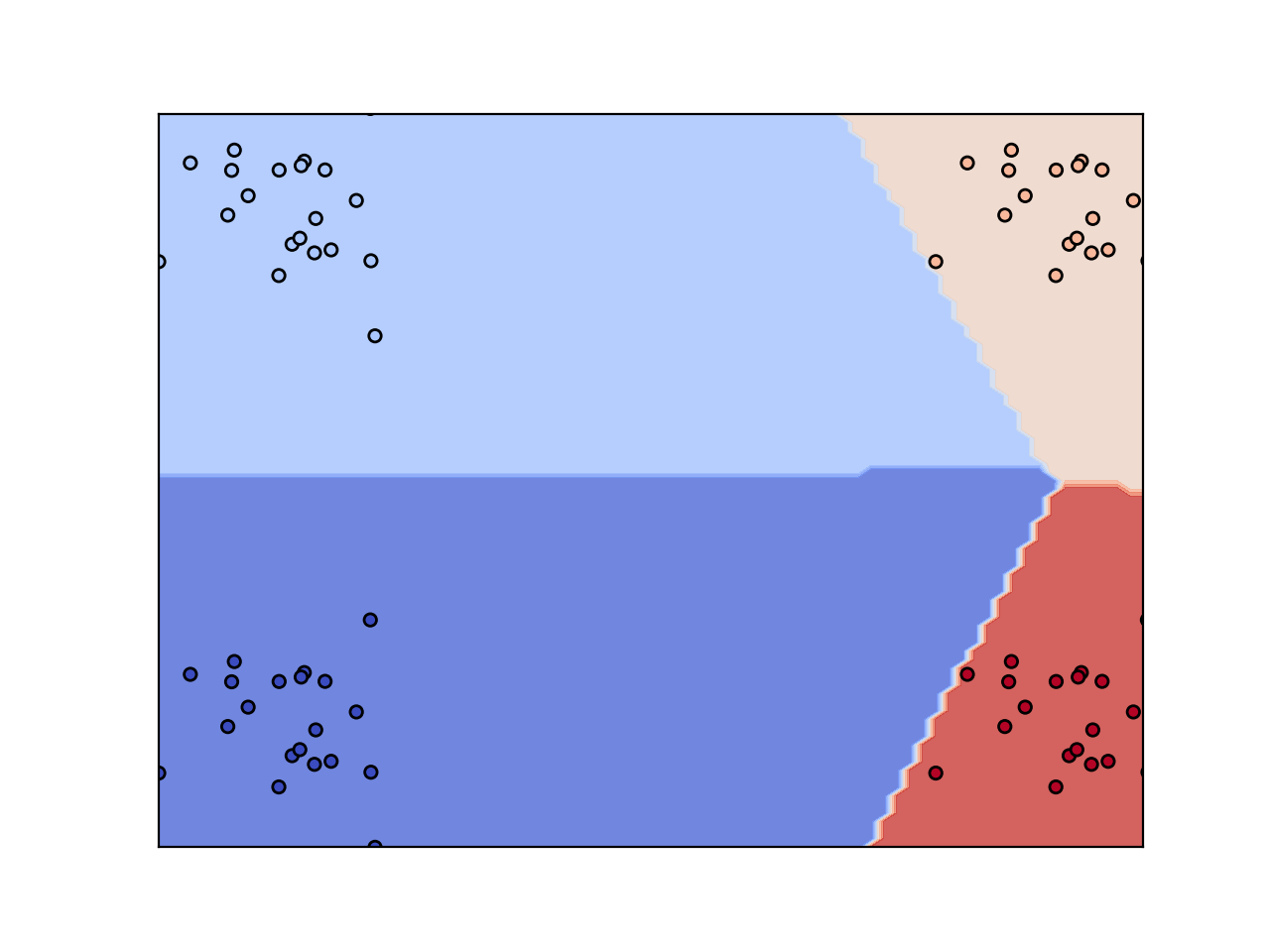
Figure 2: An example of a desired decision boundary with priority vector $\{10,10,1,1\}$.

Fisher consistency.

Define $P_{j}(x)=P(Y=j|X=x)$, and a classifier with loss $\ell(f(x),y)$ is Fisher consistent if the minimizer of $E_{P}[\ell(f(x),y)]$ has the property $\text{argmax}_{j}f_{j}=\text{argmax}_{j}P_{j}$. Although the binary SVM is known to be Fisher consistent, not all MSVMs are. In particular, in Table 1 rows $1-3$ are known to not always be consistent. In contrast, row 5 is always Fisher consistent when $\gamma\in[0,0.5]$, which also covers row 4 as a special case with $\gamma=0$ (Liu, 2007). Recall that the cost function of the cost-sensitive classification problem is the sum over all classes of the probability of erring on that class times the weight assigned to that class; we will define a cost-sensitive classifier to be Fisher consistent if the minimizer of $E_{P}[\ell(f(x),y)]$ has the property $\text{argmax}_{j}f_{j}=\text{argmax}_{j}\theta_{j}P_{j}$ . In Section 3 we prove that the our algorithm is cost-sensitive Fisher consistent.

2 The apportioned margin framework

Given a cost sensitive problem, a desired property for our classifier is to impose larger margins for the more “expensive” labels. Our cost-sensitive framework allows for a flexible method for shifting the decision boundary between different pairs of classes. Intuitively, we “budget” the regions between conflicting classes according to some priority vector. This goal is illustrated graphically in Figure 2: The two classes on the left have identical costs, but their cost is greater than that of the two classes on the right, which also have identical costs. As a result, the horizontal boundaries are centered, but the vertical boundaries are shifted to the right. As shown in the experimental section Figure 5, the widely used methods for cost sensitive multi-classification do not achieve this.

In binary SVM, the solution vector w defines a separator, whose margin depends on $\left\lVert\text{{\bf{w}}}\right\rVert$. At the two edges of the margin lie the hyperplanes $\text{{\bf{w}}}\cdot\text{{\bf{x}}}\pm 1=0$. If we were to denote $\text{{\bf{w}}}=\text{{\bf{w}}}_{+}=-\text{{\bf{w}}}_{-}$ as two classifiers for the positive and negative examples respectively, then the binary hyperplanes can be reformulated as $\text{{\bf{w}}}_{j}x=1$ and the decision function $\hat{y}=\text{argmax}_{j}\text{{\bf{w}}}_{j}x$. (See Figure 1 (a)). Conversely if we were to scale the samples with $\theta_{j}$ and shift the decision boundary by a ratio of $\frac{\theta_{+}}{\theta_{-}}$ (which is also the ratio between their Bayesian probabilities), then the hyperplanes could be formulated as $\text{{\bf{w}}}_{j}x=\theta_{j}$ and the decision function $\text{sign}(\text{{\bf{w}}}x)$ written as $\hat{y}=\text{argmax}_{j}\frac{\text{{\bf{w}}}_{j}x}{\theta_{j}}$. Fortunately, this formulation can be extended to multiclass categorization.

By analogy to the binary hard-margin setting, we assume that each hyperplane separates its class from all others. While in the binary SVM settings the two hyperplanes are parallel, in the more general multiclass problem the different hyperplanes can intersect (see Figure 1 (c)). Consider two hyperplanes $\text{{\bf{w}}}_{i},\text{{\bf{w}}}_{j}$ separating classes $i,j$. The decision boundary between them is a bisecting hyperplane. We desire that the ratio $\frac{\theta_{i}}{\theta_{j}}$ define the distance from a weighted bisector to the hyperplanes, meaning that the ratio of the scaled distance of the weighted bisector from class $i$ to its distance from class $j$ should be $\frac{\theta_{i}}{\theta_{j}}$. (A weighted bisector is illustrated in Figure 1.) The following lemma formalizes the geometric intuition of the interaction between two neighboring classes.

Definition 1

Let $w^{ij}=w_{i}-w_{j}$, $\overline{w}_{j}=\frac{\text{{\bf{w}}}_{j}}{\theta_{j}}$ and $\bar{w}^{ij}=\bar{w}_{i}-\bar{w}_{j}$.

Lemma 1

The set of all points whose ratio of scaled distances from the hyperplanes $\text{{\bf{w}}}_{i}\cdot\text{{\bf{x}}}=\theta_{i}$ and $\text{{\bf{w}}}_{j}\cdot\text{{\bf{x}}}=\theta_{j}$ is $\frac{\theta_{i}}{\theta_{j}}$, is given by the hyperplane $\overline{w}_{ij}\text{{\bf{x}}}=0$.

Proof

$\frac{\text{{\bf{w}}}_{j}\cdot\text{{\bf{x}}}-\theta_{j}}{\text{{\bf{w}}}_{i}\cdot\text{{\bf{x}}}-\theta_{i}}=\frac{\theta_{j}}{\theta_{i}}\implies\overline{w}_{j}\cdot\text{{\bf{x}}}-1=\overline{w}_{i}\cdot\text{{\bf{x}}}-1\implies(\overline{w}_{j}-\overline{w}_{i})\text{{\bf{x}}}=\overline{w}^{ij}\text{{\bf{x}}}=0.$

Lemma 1 gives the decision rule between two classes $i,j$, and implies that our overall decision function is

$$\hat{y}=\text{argmax}_{l\in[k]}\overline{w}_{l}\cdot\text{{\bf{x}}}.$$ (5)

2.1 The Optimization Formulation

Taking $\theta_{y}$ to be the cost of making a mistake on label $y$ implies the following loss on the example-label pair $(\text{{\bf{x}}},y)$:

$$\begin{split}&L(\text{{\bf{x}}},y)={\begin{cases}\theta_{y},&{\text{if }}\max\{\overline{w}_{l}\}\cdot\text{{\bf{x}}}-\overline{w}_{y}\cdot\text{{\bf{x}}}>0\\ 0&{\text{otherwise}}.\end{cases}}\end{split}$$ (6)

As desired, this loss function is asymmetric and discourages error on relatively “important” classes. Unfortunately this problem subsumes that of minimizing zero-one loss, which known to be NP hard (Hoffgen et al., 1995). Instead we propose the following convex relaxation:

$$\begin{split}&\tilde{L}_{j}(\text{{\bf{x}}},y)={\begin{cases}\theta_{y}-\bar{\delta}_{y,j}\text{{\bf{w}}}_{j}\cdot\text{{\bf{x}}},&{\text{if }}\theta_{y}\geq\bar{\delta}_{y,j}\text{{\bf{w}}}_{j}\cdot\text{{\bf{x}}}\\ 0&{\text{otherwise }}\end{cases}}\\ &\tilde{L}(\text{{\bf{x}}},y)=\sum_{j}\tilde{L}_{j}(\text{{\bf{x}}},y),\end{split}$$ (7)

where $\bar{\delta}_{y_{i},j}$ is the signed Kronecker delta:

$$\bar{\delta}_{y,j}={\begin{cases}+1,&{\text{if }}\quad y=j\\ -1,&{\text{otherwise. }}\\ \end{cases}}$$ (8)

This relaxation is a multiclass analogue of the hinge loss, with a zero penalty above a certain margin threshold and a linearly increasing penalty below it.

It is easy to see that $\tilde{L}(\text{{\bf{x}}},y)\geq L(\text{{\bf{x}}},y)$. Note that in this formulation of the cost, an example belonging to class $j$ is charged not only for a misclassification by its own classifier $j$, but is also charged when a different classifier $i$ is not within a scaled distance of $\theta_{i}+\theta_{j}$ of the example in $j$. This results in a margin shift.

Primary Formulation.

As suggested in the previous section, in the separable case we want all examples of class $j$ to be above the plane $w_{j}x+b_{j}=\theta_{j}$. The following optimization problem is a natural multiclass analogue of hard-margin maximization:

$$\min ||W||^{2}$$ (9)

$$s.t. \bar{\delta}_{y_{i},j}(\text{{\bf{w}}}_{j}\cdot\text{{\bf{x}}}_{i}+b_{j})\geq\theta_{y_{i}}$$

Indeed, $||W||^{2}$ bounds the sum of the pairwise margins:

Lemma 2

$\sum_{s}\sum_{r<s}\left\lVert\text{{\bf{w}}}^{rs}\right\rVert^{2}\leq k\left\lVert W\right\rVert^{2}$.

Proof

Let us define $\sum_{r=1}^{k}\text{{\bf{w}}}_{r}=\text{{\bf{c}}}$. Then $\left\lVert\text{{\bf{c}}}\right\rVert^{2}=(\sum_{r=1}^{k}\text{{\bf{w}}}_{r})(\sum_{r=1}^{k}\text{{\bf{w}}}_{r})=\sum_{r=1}^{k}\left\lVert\text{{\bf{w}}}_{r}\right\rVert^{2}+2\sum_{s}\sum_{r<s}\text{{\bf{w}}}_{r}\cdot\text{{\bf{w}}}_{s}$. Using this we obtain:

$$\sum_{s}\sum_{r<s}\left\lVert\text{{\bf{w}}}_{r}-\text{{\bf{w}}}_{s}\right\rVert^{2} =(k-1)\sum_{r=1}^{k}\left\lVert\text{{\bf{w}}}_{r}\right\rVert^{2}-2\sum_{s}\sum_{r<s}\text{{\bf{w}}}_{r}\cdot\text{{\bf{w}}}_{s}$$ (10)

$$=(k-1)\sum_{r=1}^{k}\left\lVert\text{{\bf{w}}}_{r}\right\rVert^{2}-(\left\lVert c\right\rVert^{2}-\sum_{r=1}^{k}\left\lVert\text{{\bf{w}}}_{r}\right\rVert^{2})$$

$$=k\sum_{r=1}^{k}\left\lVert\text{{\bf{w}}}_{r}\right\rVert^{2}-\left\lVert c\right\rVert^{2}$$

$$\leq k\sum_{r=1}^{k}\left\lVert\text{{\bf{w}}}_{r}\right\rVert^{2}=k\left\lVert W\right\rVert^{2}.$$

By relaxing the constraints we obtain the soft margin formulation.

$$\min \quad\frac{1}{2}||W||^{2}+C\sum_{ij}\xi_{ij}$$ (11)

$$s.t. \quad\theta_{y_{i}}-\bar{\delta}_{y_{i},j}(\text{{\bf{$\text{{\bf{}}}$}}}w_{j}\cdot\text{{\bf{$\text{{\bf{}}}$}}}x_{i}+b_{j})\leq\xi_{ij}\quad\forall i,j$$

$$\quad\xi_{ij}\geq 0\quad\forall i,j.$$

Dual formulation.

The primal formulation in (11) involves searching over a $d$-dimensional space. A standard transformation to the dual amounts to kernalizing the problem, rendering the search space dimension-independent. We begin the the Lagrangian formulation

$$\max\quad\mathcal{L}=\frac{1}{2}||W||^{2}+C\sum_{ij}\xi_{ij}$$ (12)

$$-\sum_{ij}\alpha_{ij}(\xi_{ij}-(\theta_{j}-\bar{\delta}_{y_{i},j}(\text{{\bf{$\text{{\bf{}}}$}}}w_{j}\cdot\text{{\bf{$\text{{\bf{}}}$}}}x_{i}+b_{j})))$$

$$-\sum_{ij}\beta_{ij}\xi_{ij}$$

$$s.t.\quad\alpha_{ij},\beta_{ij}\geq 0\quad\forall i,j.$$

Putting $\overline{\alpha}_{ij}=\alpha_{ij}\bar{\delta}_{y_{i},j}$, and and invoking the KKT conditions, we have

$$\frac{\partial\mathcal{L}}{\partial\text{{\bf{w}}}_{j}}=0\implies\text{{\bf{w}}}_{j}=\sum_{i}\overline{\alpha}_{ij}\text{{\bf{x}}}_{i}.$$ (13)

This is our analogue of the Representer Theorem (Schölkopf et al., 2001). The second KKT condition is

$$\frac{\partial\mathcal{L}}{\partial b_{j}}=0\implies\sum_{ij}\overline{\alpha}_{ij}=0$$ (14)

and can also be written as

$$\sum_{i\in j}{\alpha}_{ij}=\sum_{i\notin j}{\alpha}_{ij}.$$ (15)

Note that his equation can act as a balancer for an unbalanced sets: For a particular class $j$ the sum of weights of data belonging to $j$ equals the sum of weights of data not belonging to $j$.

The final KKT condition is: $\frac{\partial\mathcal{L}}{\partial\xi_{ij}}=0\implies\alpha_{ij}=C-\beta_{ij}\implies 0\leq\alpha_{ij}\leq C$. Using the $\overline{\alpha}$ notation we have:

$$0\leq\delta_{ij}\overline{\alpha}_{ij}\leq 1$$ (16)

Substituting the multiclass Representer Theorem 13 back into the main equation (12), we derive:

$$\max\quad\mathcal{L}=\sum_{j=0}^{k}\sum_{i=0}^{n}\alpha_{ij}\theta_{y_{i}}-\frac{1}{2}\left\lVert W\right\rVert^{2}=\sum_{j=0}^{k}(\sum_{i=0}^{n}\alpha_{ij}\theta_{y_{i}}-\sum_{i=0}^{n}\sum_{l=0}^{n}\overline{\alpha}_{ij}\overline{\alpha}_{lj}\text{{\bf{x}}}_{i}\cdot\text{{\bf{x}}}_{l})$$ (17)

$$s.t.\quad\quad\sum_{ij}\overline{\alpha}_{ij}=0.$$

It follows from the KKT conditions that:

$$\overline{\alpha}_{ij}(\theta_{y_{i}}-(\text{{\bf{$\text{{\bf{}}}$}}}w_{j}\cdot\text{{\bf{$\text{{\bf{}}}$}}}x_{i}+b_{j}))=0.$$ (18)

When $\overline{\alpha}_{ij}=0$ we have that $\theta_{y_{i}}-(\text{{\bf{$\text{{\bf{}}}$}}}w_{j}\cdot\text{{\bf{$\text{{\bf{}}}$}}}x_{i}+b_{j})\neq 0$, while if $\overline{\alpha}_{ij}\neq 0$ we have that $\theta_{y_{i}}-(\text{{\bf{$\text{{\bf{}}}$}}}w_{j}\cdot\text{{\bf{$\text{{\bf{}}}$}}}x_{i}+b_{j})=0$. The vectors $\text{{\bf{x}}}_{i}$ where $\overline{\alpha}_{ij}\neq 0$ can be considered to be the support vector for class $j$. These points lie on the hyperplane $\text{{\bf{$\text{{\bf{}}}$}}}w_{j}\cdot\text{{\bf{x}}}+b_{j}=\theta_{j}$, which is the “support hyperplane” for class $j$.

3 Statistical error bounds

In this section we will present generalization bounds. We first obtain tight bounds in the realizable case via the decision directed acyclic graph (DDAG) approach, and then present the Rademacher framework for the general (agnostic) case.

Directed Graph Approach.

Platt et al. (1999) considered a classifier for the multiclass problem, which takes the form of a binary directed acyclic graph (DAG); they termed their classifier a decision DAG (DDAG). Each class is represented as a terminal node in the graph, and given a test point, the algorithm begins at root of the graph and traverses down towards a terminal. At each node, two classes are considered, and each exiting path cannot reach one of the classes, meaning that the decision made at the node will effectively rule out one class from consideration. It follows that the DDAG has depth $k-1$. It is immediate that the DDAG can be used to model our decision function with depth $k-1$ and $k-1$ nodes for each class, where we use $\bar{w}^{ij}$ to decide between pairs of classes. The generalization bounds presented in Platt et al. (1999) for a given label is:

Theorem 3.1 (Platt et al. (1999))

Suppose we are able to correctly distinguish class $i$ from all other classes in a random $n$ sample of labeled examples using a SVM DDAG on $k$ classes with margin $\gamma_{ij}$ at node ${i,j}$, then we can bound the generalization error on class $i$ with probability greater than $1-\delta$ to be less than

$$\epsilon(i)\leq\frac{130R^{2}}{n}(D\log{4en}\log{4n}+\log{\frac{2(2n)^{k-1}}{\delta}}),$$ (19)

where $R$ is the radius of a ball containing the support of the distribution and $D=\sum_{j}\frac{1}{\gamma_{ij}^{2}}$.

As an immediate corollary of Theorem 3.1 we have:

Corollary 1

Suppose we are able to correctly distinguish between all $k$ classes in a random $n$ sample of cost sensitive labeled examples using a SVM DDAG with margin $\gamma_{ij}$ at node ${i,j}$. Then we can bound the total loss to be less than $\sum_{i}\theta_{i}\epsilon(i)$.

In both Theorem 3.1 and its corollary, $\gamma_{ij}$ is the margin between class $i$ and the separating hyperplane between class $i$ and class $j$: $\gamma_{ij}=\min_{x\in i}\frac{(\overline{w}_{i}-\overline{w}_{j})\text{{\bf{x}}}}{\left\lVert\overline{w}^{i,j}\right\rVert}$. Let $\eta_{ij}=\frac{\theta_{i}}{\theta_{j}}$, and we can bound $\gamma_{ij}$ as follows:

Lemma 3

The margin $\gamma_{ij}=\min_{x\in i}\frac{(\overline{w}_{i}-\overline{w}_{j})\text{{\bf{x}}}}{\left\lVert\overline{w}^{i,j}\right\rVert}$ statisfies $\gamma_{ij}\geq\frac{1+\eta_{ij}}{\left\lVert\overline{w}^{ij}\right\rVert}$.

Proof

By definition, $\gamma_{ij}=\min_{x\in i}\frac{(\overline{w}_{i}-\overline{w}_{j})\text{{\bf{x}}}}{\left\lVert\overline{w}^{i,j}\right\rVert}.$ From the constraints we have both that $\theta_{y}-\text{{\bf{w}}}_{y}\cdot\text{{\bf{x}}}\leq 0\implies\text{{\bf{w}}}_{y}\cdot\text{{\bf{x}}}\geq\theta_{y}$ and $\theta_{y}+\text{{\bf{w}}}_{j}\cdot\text{{\bf{x}}}\leq 0\implies-\text{{\bf{w}}}_{j}\cdot\text{{\bf{x}}}\geq\theta_{y}$, $\forall y\neq j.$ It follows that $(\overline{w}_{i}-\overline{w}_{j})\text{{\bf{x}}}\geq\frac{\theta_{i}}{\theta_{i}}+\frac{\theta_{i}}{\theta_{j}}=1+\eta_{ij}$, and we conclude that $\gamma_{ij}\geq\frac{1+\eta_{ij}}{\left\lVert\overline{w}^{ij}\right\rVert}$.

Note that when $\theta_{i}\gg\theta_{j}$, the error on the $i$-th class becomes small, as desired.

Rademacher complexity.

Let $f_{j}$ be a function mapping $(\text{{\bf{x}}},y)$ to $\mathbb{R}$ via $f_{j}(\text{{\bf{x}}},y)=[\theta_{y}\pm\text{{\bf{w}}}_{j}\cdot\text{{\bf{x}}}]_{+}$, where $\theta_{y}=\theta(y)$ is a fixed function $\theta:[k]\to\mathbb{R}_{+}$ mapping the labels to positive reals, $\text{{\bf{x}}},\text{{\bf{w}}}_{j}\in\mathbb{R}^{d}$ have Euclidean norm at most $R$ and $\Lambda_{j}$, respectively. Let us bound the Rademacher complexity of the function class $F_{j}$ of all such $f_{j}$ indexed by the $\text{{\bf{w}}}_{j}$, restricted to the given range of x:

$$R_{n}(F_{j}) =\mathbb{E}\sup_{\text{{\bf{w}}}_{j}}\frac{1}{n}\sum_{i=1}^{n}\sigma_{i}[\theta(y_{i})\pm\text{{\bf{w}}}_{j}\cdot\text{{\bf{x}}}_{i}]_{+}$$ (20)

$$\leq\mathbb{E}\sup_{\text{{\bf{w}}}_{j}}\frac{1}{n}\sum_{i=1}^{n}\sigma_{i}(\theta(y_{i})\pm\text{{\bf{w}}}_{j}\cdot\text{{\bf{x}}}_{i})$$

$$=\mathbb{E}\frac{1}{n}\sum_{i=1}^{n}\sigma_{i}\theta(y)+\mathbb{E}\sup_{\text{{\bf{w}}}_{j}}\frac{1}{n}\sum_{i=1}^{n}\sigma_{i}\text{{\bf{w}}}_{j}\cdot\text{{\bf{x}}}_{i}$$

$$\leq\frac{1}{n}\sum_{i=1}^{n}\theta(y)\mathbb{E}\sigma_{i}+\mathbb{E}\sup_{\text{{\bf{w}}}_{j}}\frac{1}{n}\sum_{i=1}^{n}\sigma_{i}\text{{\bf{w}}}_{j}\cdot\text{{\bf{x}}}_{i}$$

$$=\mathbb{E}\sup_{\text{{\bf{w}}}_{j}}\frac{1}{n}\sum_{i=1}^{n}\sigma_{i}\text{{\bf{w}}}_{j}\cdot\text{{\bf{x}}}_{i}\leq\frac{R\Lambda_{j}}{\sqrt{n}},$$

where the first inequality follows from the Talagrand contraction lemma (Mohri et al., 2012, Lemma 4.2), (Ledoux and Talagrand, 1991, Theorem 4.12), and the second from standard Rademacher estimates on linear classes (Mohri et al., 2012, Theorem 4.3).

The error margin for class $j$ is proportional to $\Lambda_{j}$ which is inverse proportional to margin of class $j$ and as proven in the previous section our method sets the margins to be proportional to the $\theta$’s and hence the more costly examples have tighter bounds, which is the desired effect.

Finally, consider the function classes $F_{j}$, $j\in[k]$, each parametrized by $\text{{\bf{w}}}_{j}$ with Euclidean norm at most $\Lambda_{j}$. Define $F$ as the (Minkowski) sum of these classes:

$$F=\left\{(\text{{\bf{x}}},y)\mapsto\sum_{j=1}^{k}f_{j}(\text{{\bf{x}}},y):f_{j}\in F_{j}\right\}$$

and recall that Rademacher complexities are sub-additive. Then

$$R_{n}(F)\leq\frac{R\sum_{j=1}^{k}\Lambda_{j}}{\sqrt{n}}\leq R||W||\sqrt{\frac{k}{n}}.$$

This explains why in the optimization formulation we minimized $||W||_{2}^{2}$.

Let us clip our loss at $\theta_{\max}$, so $\tilde{L}^{\prime}:=\min\left\{\tilde{L},\theta_{\max}\right\}$. Then, by (Mohri et al., 2012, Theorem 3.1), we have that with probability $\geq 1-\delta$,

$$\mathbb{E}_{(X,Y)}[\tilde{L}^{\prime}(X,Y)]\leq\frac{1}{n}\sum_{i=1}^{n}\tilde{L}^{\prime}(X_{i},Y_{i})+2R_{n}(\min\left\{\theta_{\max},F\right\})+\theta_{\max}\sqrt{\frac{\log(1/\delta)}{2n}}.$$

Since truncation by $\theta_{\max}$ is a $1$-Lipschitz transformation, the Talagrand contraction lemma implies that $R_{n}(\min\left\{\theta_{\max},F\right\})\leq R_{n}(F)$, if we also normalize the loss function w.l.o.g. by $\theta_{\max}$ we obtain our final bound,

$$\mathbb{E}_{(X,Y)}[\tilde{L}^{\prime}(X,Y)]\leq\frac{1}{n}\sum_{i=1}^{n}\tilde{L}^{\prime}(X_{i},Y_{i})+2R\frac{||W||}{\theta_{\max}}\sqrt{\frac{k}{n}}+\sqrt{\frac{\log(1/\delta)}{2n}},$$

which holds with probability $\geq 1-\delta$.

3.1 Fisher Consistency

Given the set of functions $F_{j}$ we will say that a classifier with loss $\ell(f(x),y)$ is Fisher consistent if the minimizer of $E_{P}[\ell(f(x),y)]$ has the property $\text{argmax}_{j}f_{j}=\text{argmax}_{j}\theta_{j}P_{j}$. We note that this ensures the intuitive property that for point $(x,y)$ we have $\frac{P_{y}(x)}{P_{j}(x)}\geq\frac{\theta_{j}}{\theta_{y}}\quad\forall j\neq y$. In order to prove the our classifier is Fisher consistent, without loss of generality we impose the additional constraint that $\sum f_{j}(x)=0$.

Lemma 4

The minimizer $\mathbb{f}^{*}$ of $E_{p}[\sum_{j=1}^{k}[\theta_{y}-\overline{\delta}_{y,j}f_{j}]_{+}]$ subject to $\sum_{j=1}^{k}f_{j}=0$ satisfies the following: $f^{*}_{j}(x)=\theta_{j}$ if $j=\text{argmax}_{j}\theta_{j}P_{j}(x)$ and $-\frac{\theta_{j}}{k-1}$ otherwise.

Proof

By defintion, $E[\sum_{j=1}^{k}[\theta_{y}-\overline{\delta}_{y,j}f_{j}]_{+}]=\sum_{l}P_{l}\sum_{j}[\theta_{l}-\overline{\delta}_{l,j}f_{j}]_{+}$. We first show that the minimizer $\text{{\bf{f}}}^{*}$ for point $(\text{{\bf{x}}},y)$ satisfies $\overline{\delta}_{y,j}f_{j}^{*}\leq\theta_{y}\quad\forall y,j$. Suppose by way of contradiction that the optimal solution $\text{{\bf{f}}}^{*}$ has $\overline{\delta}_{y,j}f_{j}>\theta_{y}$ for some $j$; then we can construct another solution $\text{{\bf{f}}}^{\prime}$ with $f_{j}^{\prime}=\overline{\delta}_{y,j}\theta_{y}$ and $f_{l}^{\prime}=f_{l}^{*}+\frac{f_{j}^{\prime}-\overline{\delta}_{y,j}\theta_{y}}{k-1}\quad\forall l\neq j$. The second solution satisfies $\overline{\delta}_{y,j}f_{j}^{\prime}\geq\overline{\delta}_{y,j}f_{j}^{*}$ while still satisfying the constraint $\sum f_{j}^{*}=\sum f_{j}^{\prime}$, However the objective function $\sum_{j=1}^{k}[\theta_{y}-\overline{\delta}_{y,j}f^{\prime}_{j}]_{+}\leq\sum_{j=1}^{k}[\theta_{y}-\overline{\delta}_{y,j}f^{*}_{j}]_{+}$, which is a contradiction.

Using this property of $f^{*}$, we can rewrite the objective function as $\sum_{l}P_{l}\sum_{j}\theta_{l}-\overline{\delta}_{l,j}f_{j}$. Since $\sum f_{j}=0$ implies $\sum\overline{\delta}_{y,j}f_{j}=2f_{j}$, and then the objective function can be written as: $\sum_{l}P_{l}\sum_{j}\theta_{l}-\overline{\delta}_{l,j}f_{j}=\sum_{l}P_{l}\sum_{j}\theta_{l}-2f_{j}$ which is equivalent to:

$$\text{max}_{F_{j}}\sum P_{l}f_{l}$$

$$s.t.\quad\sum f_{j}=0\quad f_{j}\overline{\delta}_{jl}\leq\theta_{j}\quad\forall j$$

If we define $\hat{y}=\text{argmax}_{j}\theta_{j}P_{j}$, it is easy to see that the solution satisfies $f^{*}_{\hat{y}}=\theta_{\hat{y}}$ and $-\frac{\theta_{\hat{y}}}{k-1}$ otherwise.

4 SGD Based Solver

In this section, we present a Stochastic Gradient Descent (SGD) based learning algorithm for solving our algorithm. Although SGD based algorithms are not the optimized solution for convex problems, the are widely used in non convex problems such as NeuralNets. Initially, we set each $\text{{\bf{w}}}_{j}$ to the zero vector, At iteration $t$ of the algorithm, we choose a random training example $(\text{{\bf{x}}}_{t},y_{t})$ by picking an index uniformly at random and compute the sub-gradient

$$\nabla_{t,j}\mathcal{L}=\lambda\text{{\bf{w}}}_{j,t}-\mathds{1}[\theta_{y_{t}}-\bar{\delta}_{y_{t},j}\text{{\bf{w}}}_{j,t}\text{{\bf{x}}}_{t}]\bar{\delta}_{y_{t},j}\text{{\bf{w}}}_{j,t}\text{{\bf{x}}}_{t},$$ (21)

where $\mathds{1}[.]$ is the indicator function (which takes a value of 1 if its argument is positive and zero otherwise).

The update rule is $\text{{\bf{w}}}_{j,t+1}\leftarrow\text{{\bf{w}}}_{j,t}-\eta_{t}\nabla_{t,j}$, where $\eta_{t}$ is the step size at iteration t. Following the Shalev-Singer Pegasos implementation (Shalev-Shwartz et al., 2011) we take $\eta_{t}=\frac{1}{\lambda_{t}}\quad\lambda_{t}=\lambda\cdot t$, and then the update rule can therefore be rewritten as:

$$\text{{\bf{w}}}_{j,t+1}\leftarrow\underbrace{(1-\frac{1}{t})\text{{\bf{w}}}_{j,t}}_{*}-\underbrace{\frac{1}{\lambda_{t}}\mathds{1}[\theta_{y_{t}}-\bar{\delta}_{y_{t},j}\text{{\bf{w}}}_{j,t}\text{{\bf{x}}}_{t}]\bar{\delta}_{y_{t},j}\text{{\bf{x}}}_{t}}_{**}.$$ (22)

Here (*) can be viewed as a momentum term, smoothing through past results, and (**) applies a $\frac{1}{t}$ weight decay over the gradient of the loss function. The algorithm achieves $\epsilon$-accuracy in time $\mathcal{O}(\frac{1}{\lambda\epsilon})$. Note, that unlike other cost sensitive implementations, an example belonging to class $j$ does not only affect $\text{{\bf{w}}}_{j}$ but also affects all other w’s as well by forcing them to retain a scaled margin from that example.

Dual problem.

This result can be generelized to apply Mercer’s kernel. The multiclass Representer Theorem (13) gives:

$$\text{{\bf{w}}}_{j}=\sum_{i=0}^{n}\overline{\alpha}_{i,j}\text{{\bf{x}}}_{i}$$ (23)

This implies that the optimal solution can be expressed as a linear combination of the training instances, making it possible to train and utilize an SVM without direct access to the training instances. In this case, solving the dual problem is not necessary since we can directly minimize the primal while still using kernels:

$$\text{{\bf{w}}}_{j,t+1}=\frac{1}{\lambda_{t}}\sum_{i=0}^{t}\mathds{1}[\theta_{y_{t}}-\bar{\delta}_{y_{t},j}\text{{\bf{w}}}_{j,t}\cdot\phi(x_{t})]\bar{\delta}_{y_{t},j}\phi(x_{t}).$$ (24)

We can now combine equations (24) and (13) to get the following lemma:

Lemma 5

The weight at stage $t+1$ is given by:

$$\text{{\bf{w}}}_{j,t+1}=\frac{1}{\lambda_{t}}\sum_{i=0}^{n}\overline{\alpha}_{i,j,t+1}\phi(x_{i}),$$ (25)

where $\overline{\alpha}_{i,j,t+1}$ is given by:

$$\overline{\alpha}_{i,j,t}+{\begin{cases}\delta_{i,x_{t}}\bar{\delta}_{y_{t},j},&{\text{if }}\theta_{y_{t}}>\frac{\bar{\delta}_{y_{t},j}}{\lambda_{t}}\sum_{i=0}^{n}\overline{\alpha}_{i,j,t}K(\text{{\bf{x}}}_{i},\text{{\bf{x}}}_{t})\\ 0&{\text{otherwise. }}\end{cases}}$$ (26)

Proof

. We prove the equation by induction. Suppose the update rule holds for $t-1$, then:

1. When the indicator function is zero the update rule is:

   $$\text{{\bf{w}}}_{j,t+1}=\frac{t-1}{t}\text{{\bf{w}}}_{j,t}=\frac{t-1}{t}\frac{1}{\lambda_{t-1}}\sum_{i=0}^{n}\overline{\alpha}_{i,j,t}\phi(\text{{\bf{x}}}_{i})$$ (27)

   $$=\frac{1}{\lambda_{t}}\sum_{i=0}^{t}\overline{\alpha}_{i,j,t}\phi(\text{{\bf{x}}}_{i})$$

2. When the indicator function is non-zero then:

   $$\text{{\bf{w}}}_{j,t+1}=\frac{1}{\lambda_{t}}\sum_{i=0}^{n}\overline{\alpha}_{i,j,t}\phi(\text{{\bf{x}}}_{i})+\frac{1}{\lambda_{t}}\bar{\delta}_{y_{t},j}\phi(x_{t})$$ (28)

   $$=\frac{1}{\lambda_{t}}\sum_{i=0}^{n}(\overline{\alpha}_{i,j,t}+\delta_{i,x_{t}}\bar{\delta}_{y_{t},j})\phi(\text{{\bf{x}}})$$

Combining equations (26) and (28) we proved the update rule.

The final decision function is:

$$\hat{y}=\text{argmax}_{j}\frac{1}{\theta_{j}}\sum_{i=0}^{n}\overline{\alpha}_{i,j}K(\text{{\bf{x}}}_{i},x)$$ (29)

This is a simple and elegant update rule which only depends on the vector $\theta$ and $K(,)$.

5 Experiments

For our experiments, we utilized the python scikit-learn library (Pedregosa et al., 2011) and our own SGD implementation . We used SVM RBF kernel, the regularization parameter $C$ was 5-fold cross-validated over the set $\{2^{-5},2^{-3},\ldots,2^{15}\}$, and the gamma parameter was 5-fold cross-validated over the set $\{2^{-15},2^{-3},\ldots,2^{3}\}$.

5.1 Illustrative example

Before presenting the experiments, we give an example that illustrates the power of our approach. We generated 2-dimensional data from four separable classes with different biases, and generated their data points using a normal distribution. Figure 3 shows a comparison of the results of different cost vectors. This example illustrates how our approach shifts the decision boundary away from high-cost classes, while still maintaining the convexity of the solution space.

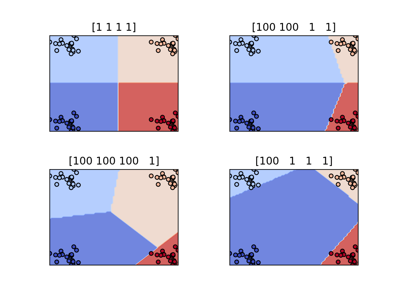
Figure 3: Separating classes with different prioritization vectors assigned to classes {blue, light blue, yellow, red}.

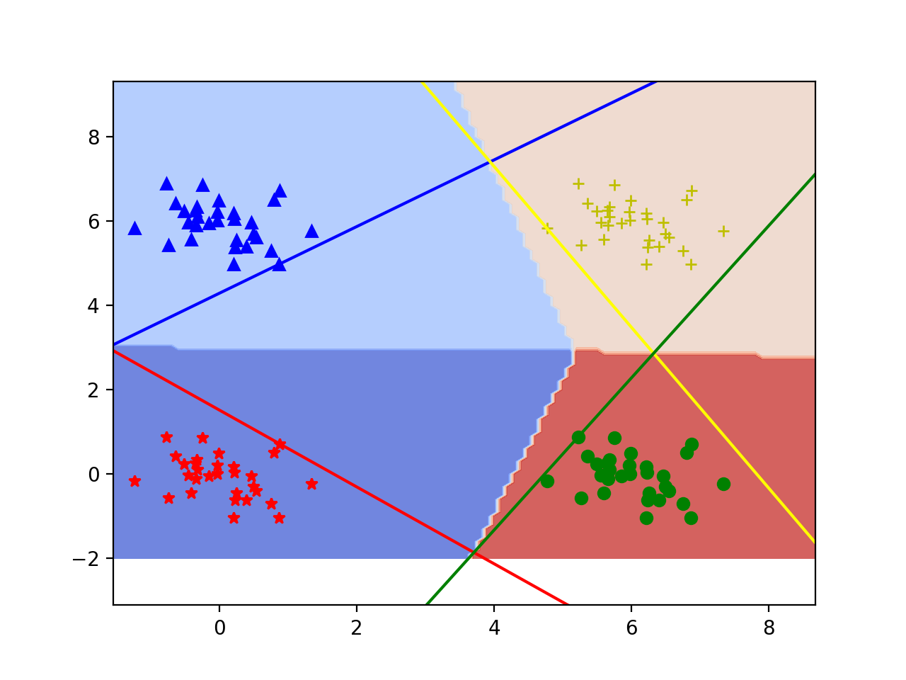
Figure 4: Decision boundary and the $w_{j}x+b_{j}=\theta_{j}$ hyperplanes.

We also compared our result against the CSOVO, CSOVA and CSCS methods described in Section 1.1. Figure 5 shows a comparison of these different methods for the same cost vector. It is evident that the other methods were unable to significantly shift the decision boundary away from the high-cost classes.

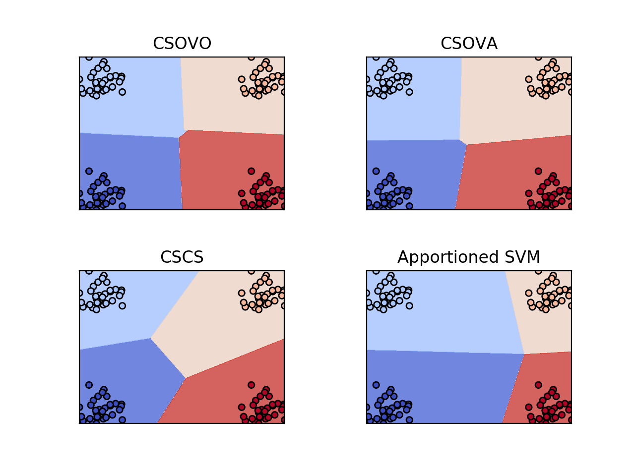
Figure 5: A comparison of decision boundaries between different algorithms for priority vector $\{10,10,1,1\}$.

5.2 Benchmarks

We considered various benchmark datasets from LibSVM Machine Learning repository (Chang and Lin, 2011). Three of these (Heart , Breast, Diabetes) are healthcare-oriented datasets where the prioritization is inherent (false positives are preferred over false negatives). We set the cost vector for the more important class to be twice than the rest for all datasets except for German Credit (Statlog), where the cost vector of $\{5,1\}$ was already stipulated by the authors. We also considered several multicategorial datasets, and randomly chose one of the classes to be more important than the others. The datasets characteristics are summarized in Table 5.2

The reported score is expected risk (the sum of the number of misclassification for each class times its cost, normalized by the data size). Results were averaged over 10-fold cross validation. We compared our method against other weighted multiclass methods, and the results are presented in Table 2. Our method compares favorably with the others reducing the cost by $10-20\%$. We also report the sensitivity of the most important class. These show empirically that, as claimed, our method successfully increased the sensitivity of the most important class, and did this more effectively than all other methods.

tableDataset characteristics #classes #examples #dims Breast Cancer 2 683 10 Diabetes 2 768 8 Heart 2 270 13 German 2 1000 20 Glass 6 214 9 Iris 3 150 4 Vehicle 4 846 18 Letter 26 20000 16

Dataset	our SVM	CSOVA	CSCS	CSOVO
Breast	0.058	0.054	0.056	0.054
	86%	84%	83%	84%
Diabetes	0.343	0.353	0.346	0.351
	77%	74%	74%	74%
Heart	0.215	0.218	0.214	0.218
	80%	81%	80%	81%
German	0.250	0.300	0.3000	0.300
	74%	70%	70%	70%
Iris	0.033	0.053	0.043	0.053
	97%	95%	93%	95%
Glass	0.491	0.501	0.495	0.501
	74%	63%	65%	63%
Vehicle	0.262	0.281	0.272	0.281
	76%	64%	62%	60%
Letter	0.067	0.231	0.173	0.231
	96%	91%	91%	91%

Table 2: Benchmarks for cost-sensitive classification

5.3 Cost Sensitive NeuralNets

The results of the linear classifiers encourage us to adapt the framework to neural networks (NNs), as cost-sensitive NNs are not well-understood. A naive approach could simply multiply the output of the final loss layer (usually a softmax layer) by the appropriate weights, but this leads to poor performance (Table 3). Kukar and Kononenko (1998) suggested the cost function $\sum_{j=0}^{k}\sum_{i=0}^{n}((y_{j}-o_{j})C(i,j))^{2}$ where $o_{j}$ is the actual output of the $j$-th output neuron, $y_{j}$ is the desired output, and $C(i,j)$ is the cost for misclassifying example $i$ as $j$.

We executed the following experiment on the use of NNs to identify superclasses. We used the CIFAR-100 dataset, a dataset of small images each labelled with a class, where all classes are themselves grouped into superclasses. For our experiment, we chose two superclasses and two subclasses for each superclass. These were superclass aquatic mammals with subclasses dolphin and beaver, and superclass flower with subclasses orchid and sunflower. Our prioritization vector was $\{1,1,2,2\}$, assigning double priority to aquatic mammals. Each subclass had 500 training images and 100 testing images. Our premise was that that our cost function could be used to improve image recognition via classes, that is to train a classifier to favor misclassifying a dolphin as a beaver over a dolphin as an orchid.

For a more detailed description of the NeuralNet architecture: The architecture of our net is summarized in Figure 6. The net is similar to the one introduced by Krizhevsky et al. (2017) also known as “AlexNet”: It contains three convolutional layers and two fully connected layers, each followed by a batch normalization (BN) and dropout layers with probability $0.75$. We used ReLU as our activation function. The first layer CONV-1 uses a kernel of $5\times 5\times 24$ with stride $1$ . The second layer CONV-2 uses a kernel of $5\times 5\times 48$ with stride $2$. The third layer CONV-3 uses a kernel of $4\times 4\times 64$ with stride $2$. The fourth layer is a 200 neurons fully connected layer (FC) followed by a hinge loss (HL). In the final layer we compared three different possible tools, the regular cross entropy with softmax and class weighting, SVM hinge-loss with class weighting and our prioritization loss. We trained our models using Adam gradient descent (Kingma and Ba, 2015) with a batch size of 100 examples and an exponential weight decay.

Figure 6: Network Architecture

Our final result are presented in Table 3, which shows the overall cost function, and also the sensitivity of the preferred superclass (aquatic mammals), for NNs utilizing the different algorithms (Weighted softmax , Weighted Hinge loss , Apportioned margin loss).

Method	Sensitivity	Cost
Weighted softmax	81.5%	0.186
Weighted Hinge loss	80.5%	0.201
Apportioned margin loss	86%	0.153

Table 3: Superclass experiment

6 Conclusions

We introduced the apportioned margin framework which places the cost on the margins rather than on misclassification. This framework guarantees an tighter out-of-sample error bound for more important classes sometime at the expense of less important classes according to a user-defined priority vector. We presented both linear, kernelized, and NeuralNet vesrsions for this framework and demonstrated the success of our method on different datasets.

References

- An and Liang (2013) An W, Liang M (2013) Fuzzy support vector machine based on within-class scatter for classification problems with outliers or noises. Neurocomputing 110:101–110, DOI 10.1016/j.neucom.2012.11.023, URL https://doi.org/10.1016/j.neucom.2012.11.023
- Asif et al. (2015) Asif K, Xing W, Behpour S, Ziebart BD (2015) Adversarial cost-sensitive classification. In: UAI, AUAI Press, pp 92–101
- Bradley (1997) Bradley AP (1997) The use of the area under the ROC curve in the evaluation of machine learning algorithms. Pattern Recognition 30(7):1145–1159, DOI 10.1016/S0031-3203(96)00142-2, URL https://doi.org/10.1016/S0031-3203(96)00142-2
- Bredensteiner and Bennett (1999) Bredensteiner EJ, Bennett KP (1999) Multicategory classification by support vector machines. Comp Opt and Appl 12(1-3):53–79, DOI 10.1023/A:1008663629662, URL https://doi.org/10.1023/A:1008663629662
- van den Burg and Groenen (2016) van den Burg GJ, Groenen PJ (2016) Gensvm: A generalized multiclass support vector machine. Journal of Machine Learning Research 17(225):1–42, URL http://jmlr.org/papers/v17/14-526.html
- Chang and Lin (2011) Chang CC, Lin CJ (2011) LIBSVM: A library for support vector machines. ACM Transactions on Intelligent Systems and Technology 2:27:1–27:27, software available at http://www.csie.ntu.edu.tw/~cjlin/libsvm