Randomized Numerical Linear Algebra:
Foundations & Algorithms
Randomized Numerical Linear Algebra:
Foundations & Algorithms
Per-Gunnar Martinsson, University of Texas at Austin
Joel A. Tropp, California Institute of Technology
Abstract: This survey describes probabilistic algorithms for linear algebra computations, such as factorizing matrices and solving linear systems. It focuses on techniques that have a proven track record for real-world problems. The paper treats both the theoretical foundations of the subject and practical computational issues.
Topics include norm estimation; matrix approximation by sampling; structured and unstructured random embeddings; linear regression problems; low-rank approximation; subspace iteration and Krylov methods; error estimation and adaptivity; interpolatory and CUR factorizations; Nyström approximation of positive semidefinite matrices; single-view (“streaming”) algorithms; full rank-revealing factorizations; solvers for linear systems; and approximation of kernel matrices that arise in machine learning and in scientific computing.
1. Introduction
Numerical linear algebra (NLA) is one of the great achievements of scientific computing. On most computational platforms, we can now routinely and automatically solve small- and medium-scale linear algebra problems to high precision. The purpose of this survey is to describe a set of probabilistic techniques that have joined the mainstream of NLA over the last decade. These new techniques have accelerated everyday computations for small- and medium-size problems, and they have enabled large-scale computations that were beyond the reach of classical methods.
1.1. Classical numerical linear algebra
NLA definitively treats several major classes of problems, including
-
•
solution of dense and sparse linear systems;
-
•
orthogonalization, least-squares, and Tikhonov regularization;
-
•
determination of eigenvalues, eigenvectors, and invariant subspaces;
-
•
singular value decomposition (SVD) and total least-squares.
In spite of this catalog of successes, important challenges remain. The sheer scale of certain datasets (terabytes and beyond) makes them impervious to classical NLA algorithms. Modern computing architectures (GPUs, multi-core CPUs, massively distributed systems) are powerful, but this power can only be unleashed by algorithms that minimize data movement and that are designed ab initio with parallel computation in mind. New ways to organize and present data (out-of-core, distributed, streaming) also demand alternative techniques.
Randomization offers novel tools for addressing all of these challenges. This paper surveys these new ideas, provides detailed descriptions of algorithms with a proven track record, and outlines the mathematical techniques used to analyze these methods.
1.2. Randomized algorithms emerge
Probabilistic algorithms have held a central place in scientific computing ever since Ulam and von Neumann’s groundbreaking work on Monte Carlo methods in the 1940s. For instance, Monte Carlo algorithms are essential for high-dimensional integration and for solving PDEs set in high-dimensional spaces. They also play a major role in modern machine learning and uncertainty quantification.
For many decades, however, numerical analysts regarded randomized algorithms as a method of last resort—to be invoked only in the absence of an effective deterministic alternative. Indeed, probabilistic techniques have several undesirable features. First, Monte Carlo methods often produce output with low accuracy. This is a consequence of the central limit theorem, and in many situations it cannot be avoided. Second, many computational scientists have a strong attachment to the engineering principle that two successive runs of the same algorithm should produce identical results. This requirement aids with debugging, and it can be critical for applications where safety is paramount, for example simulation of infrastructure or control of aircraft. Randomized methods do not generally offer this guarantee. (Controlling the seed of the random number generator can provide a partial work-around, but this necessarily involves additional complexity.)
Nevertheless, in the 1980s, randomized algorithms started to make inroads into NLA. Some of the early work concerns spectral computations, where it was already traditional to use random initialization. ? recognized that (a variant of) the power method with a random start provably approximates the largest eigenvalue of a positive semidefinite (PSD) matrix, even without a gap between the first and second eigenvalue. ? provided a sharp analysis of this phenomenon for both the power method and the Lanczos algorithm. Around the same time, ? and ? proposed Monte Carlo methods for estimating the trace of a large psd matrix. Soon after, ? demonstrated that randomized transformations can be used to avoid pivoting steps in Gaussian elimination.
Starting in the late 1990s, researchers in theoretical computer science identified other ways to apply probabilistic algorithms in NLA. ? and ? showed that randomized embeddings allow for computations on streaming data with limited storage. (?) and (?) proposed Monte Carlo methods for low-rank matrix approximation. (?), (?), and (?) wrote the first statement of theoretical principles for randomized NLA. ? showed how subspace embeddings support linear algebra computations.
In the mid-2000s, numerical analysts introduced practical randomized algorithms for low-rank matrix approximation and least-squares problems. This work includes the first computational evidence that randomized algorithms outperform classical NLA algorithms for particular classes of problems. Early contributions include (?, ?, ?, ?). These papers inspired later work, such as (?, ?, ?), that has made a direct impact in applications
Parallel with the advances in numerical analysis, a tide of enthusiasm for randomized algorithms has flooded into cognate fields. In particular, stochastic gradient descent (?) has become a standard algorithm for solving large optimization problems in machine learning.
At the time of writing, in late 2019, randomized algorithms have joined the mainstream of NLA. They now appear in major reference works and textbooks (?, ?). Key methods are being incorporated into standard software libraries (?, ?, ?).
1.3. What does randomness accomplish?
Over the course of this survey we will explore a number of different ways that randomization can be used to design effective NLA algorithms. For the moment, let us just summarize the most important benefits.
Randomized methods can handle certain NLA problems faster than any classical algorithm. In Section 10, we describe a randomized algorithm that can solve a dense least-squares problem with using about arithmetic operations (?). Meanwhile, classical methods require operations. In Section 18, we present an algorithm called SparseCholesky that can solve the Poisson problem on a dense undirected graph in time that is roughly quadratic in the number of vertices (?). Standard methods have cost that is cubic in the number of vertices. The improvements can be even larger for sparse graphs.
Randomization allows us to tackle problems that otherwise seem impossible. Section 15 contains an algorithm that can compute a rank- truncated SVD of an matrix in a single pass over the data using working storage . The first reference for this kind of algorithm is ?. We know of no classical method with this computational profile.
From an engineering point of view, randomization has another crucial advantage: it allows us to restructure NLA computations in a fundamentally different way. In Section 11, we will introduce the randomized SVD algorithm (?, ?). Essentially all the arithmetic in this procedure takes place in a short sequence of matrix–matrix multiplications. Matrix multiplication is a highly optimized primitive on most computer systems; it parallelizes easily; and it performs particularly well on modern hardware such as GPUs. In contrast, classical SVD algorithms require either random access to the data or sequential matrix–vector multiplications. As a consequence, the randomized SVD can process matrices that are beyond the reach of classical SVD algorithms.
1.4. Algorithm design considerations
Before we decide what algorithm to use for a linear algebra computation, we must ask how we are permitted to interact with the data. A recurring theme of this survey is that randomization allows us to reorganize algorithms so that they control whichever computational resource is the most scarce (flops, communication, matrix entry evaluation, etc.). Let us illustrate with some representative examples:
-
•
Streaming computations (“single-view”): There is rising demand for algorithms that can treat matrices that are so large that they cannot be stored at all; other applications involve matrices that are presented dynamically. In the streaming setting, the input matrix is given by a sequence of simple linear updates that can viewed only once:
(1.1) We must discard each innovation after it has been processed. As it happens, the only type of algorithm that can handle the model (1.1) is one based on randomized linear dimension reduction (?). Our survey describes a number of algorithms that can operate in the streaming setting; see Sections 4, 5, 14, and 15.
-
•
Dense matrices stored in RAM: One traditional computational model for NLA assumes that the input matrix is stored in fast memory, so that any entry can quickly be read and/or overwritten as needed. The ability of CPUs to perform arithmetic operations keeps growing rapidly, but memory latency has not kept up. Thus, it has become essential to formulate blocked algorithms that operate on submatrices. Section 16 shows how randomization can help.
-
•
Large sparse matrices: For sparse matrices, it is natural to search for techniques that interact with a matrix only through its application to vectors, such as Krylov methods or subspace iteration. Randomization expands the design space for these methods. When the iteration is initialized with a random matrix, we can reach provably correct and highly accurate results after a few iterations; see Sections 11.6 and 11.7.
Another idea is to apply randomized sampling to control sparsity levels. This technique arises in Section 18, which contains a randomized algorithm that accelerates incomplete Cholesky preconditioning for sparse graph Laplacians.
-
•
Matrices for which entry evaluation is expensive: In machine learning and computational physics, it is often desirable to solve linear systems where it is too expensive to evaluate the full coefficient matrix. Randomization offers a systematic way to extract data from the matrix and to compute approximations that serve for the downstream applications. See Sections 19 and 20.
1.5. Overview
This paper covers fundamental mathematical ideas, as well as algorithms that have proved to be effective in practice. The balance shifts from theory at the beginning toward computational practice at the end. With the practitioner in mind, we have attempted to make the algorithmic sections self-contained, so that they can be read with a minimum of references to other parts of the paper.
After introducing notation and covering preliminaries from linear algebra and probability in Sections 2–3, the survey covers the following topics.
- •
-
•
Section 7 develops randomized sampling methods for approximating matrices, including applications to matrix multiplication and approximation of combinatorial graphs.
-
•
Sections 8–9 introduce the notion of a randomized linear embedding. These maps are frequently used to reduce the dimension of a set of vectors, while preserving their geometry. In Section 10, we explore several ways to use randomized embeddings in the context of an overdetermined least-squares problem.
- •
-
•
Section 16 develops randomized algorithms for computing a factorization of a full-rank matrix, such as a pivoted QR decomposition or a URV decomposition.
- •
- •
1.6. Omissions
While randomized NLA was a niche topic 15 years ago, we have seen an explosion of research over the last decade. This survey can only cover a small subset of the many important and interesting ideas that have emerged.
Among many other omissions, we do not discuss spectral computations in detail. There have been interesting and very recent developments, especially for the challenging problem of computing a spectral decomposition of a nonnormal matrix (?). We also had to leave out a treatment of tensors and the rapidly developing field of randomized multilinear algebra.
There is no better way to demonstrate the value of a numerical method than careful numerical experiments that measure its speed and accuracy against state-of-the-art implementations of competing methods. Our selection of topics to cover is heavily influenced by such comparisons; for reasons of space, we have often had to settle for citations to the literature, instead of including the numerical evidence.
The intersection between optimization and linear algebra is of crucial importance in applications, and it remains a fertile ground for theoretical work. Randomized algorithms are invaluable in this context, but we realized early on that the paper would double in length if we included just the essential facts about randomized optimization algorithms.
There is a complementary perspective on randomized numerical analysis algorithms, called probabilistic numerics. See the website (?) for a comprehensive bibliography.
For the topics that we do cover, we have made every effort to include all essential citations. Nevertheless, the literature is vast, and we are sure to have overlooked important work; we apologize in advance for these oversights.
1.7. Other surveys
There are a number of other survey papers on randomized algorithms for randomized NLA and related topics.
-
•
? develop and analyse computational methods for low-rank matrix approximation (including the “randomized SVD” algorithm) from the point of view of a numerical analyst. The main idea is that randomization can furnish a subspace that captures the action of a matrix, and this subspace can be used to build structured low-rank matrix approximations.
-
•
? treats randomized methods for least-squares computations and for low-rank matrix approximation. He emphasizes the useful principle that we can often decouple the linear algebra and the probability when analyzing randomized NLA algorithms.
-
•
? describes how to use subspace embeddings as a primitive for developing randomized linear algebra algorithms. A distinctive feature is the development of lower bounds.
-
•
? gives an introduction to matrix concentration inequalities, and includes some applications to randomized NLA algorithms.
-
•
The survey of ? appeared in a previous volume of Acta Numerica. A unique aspect is the discussion of randomized tensor computations.
-
•
? have updated the presentation in ?, and include an introduction to linear algebra and probability that is directed toward NLA applications.
-
•
? focuses on computational aspects of randomized NLA. A distinctive feature is the discussion of efficient algorithms for factorizing matrices of full, or nearly full, rank.
-
•
? gives a mathematical treatment of how matrix concentration supports a few randomized NLA algorithms, and includes a complete proof of correctness for the SparseCholesky algorithm described in Section 18.
1.8. Acknowledgments
We are grateful to Arieh Iserles for proposing that we write this survey. Both authors have benefited greatly from our collaborations with Vladimir Rokhlin and Mark Tygert. Most of all, we would like to thank Richard Kueng for his critical reading of the entire manuscript, which has improved the presentation in many places. Madeleine Udell, Riley Murray, James Levitt, and Abinand Gopal also gave us useful feedback on parts of the paper. Lorenzo Rosasco offered invaluable assistance with the section on kernel methods for machine learning. Navid Azizan, Babak Hassibi, and Peter Richtárik helped with citations to the literature on SGD. Finally, we would like to thank our ONR programme managers, Reza Malek-Madani and John Tague, for supporting research on randomized numerical linear algebra.
JAT acknowledges support from the Office of Naval Research (awards N-00014-17-1-2146 and N-00014-18-1-2363). PGM acknowledges support from the Office of Naval Research (award N00014-18-1-2354), from the National Science Foundation (award DMS-1620472), and from Nvidia Corp.
2. Linear algebra preliminaries
This section contains an overview of the linear algebra tools that arise in this survey. It collects the basic notation, along with some standard and not-so-standard definitions. It also contains a discussion about the role of the spectral norm.
Background references for linear algebra and matrix analysis include ? and ?. For a comprehensive treatment of matrix computations, we refer to (?, ?, ?, ?).
2.1. Basics
We will work in the real field () or the complex field (). The symbol refers to either the real or complex field, in cases where the precise choice is unimportant. As usual, scalars are denoted by lowercase italic Roman () or Greek () letters.
Vectors are elements of , where is a natural number. We always denote vectors with lowercase bold Roman () or Greek () letters. We write for the zero vector and for the vector of ones. The standard basis vectors are denoted as . The dimensions of these special vectors are determined by context.
A general matrix is an element of , where are natural numbers. We always denote matrices with uppercase bold Roman () or Greek () letters. We write for the zero matrix and for the identity matrix; their dimensions are determined by a subscript or by context.
The parenthesis notation is used for indexing into vectors and matrices: is the th coordinate of vector , while is the th coordinate of matrix . In some cases it is more convenient to invoke the functional form of indexing. For example, also refers to the th coordinate of the matrix .
The colon notation is used to specify ranges of coordinates. For example, and refer to the vector comprising the first coordinates of . The colon by itself refers to the entire range of coordinates. For instance, denotes the th row of , while denotes the th column.
The symbol ∗ is reserved for the (conjugate) transpose of a matrix of vector. A matrix that satisfies is said to be self-adjoint. It is convenient to distinguish the space of self-adjoint matrices over the scalar field. We may write if it is necessary to specify the field.
The operator † extracts the Moore–Penrose pseudoinverse of a matrix. More precisely, for , the pseudoinverse is the unique matrix that satisfies the following:
-
(1)
is self-adjoint.
-
(2)
is self-adjoint.
-
(3)
.
-
(4)
.
If has full column rank, then , where denotes the ordinary matrix inverse.
2.2. Eigenvalues and singular values
A positive semidefinite matrix is a self-adjoint matrix with nonnegative eigenvalues. We will generally abbreviate positive semidefinite to PSD. Likewise, a positive definite (PD) matrix is a self-adjoint matrix with positive eigenvalues.
The symbol denotes the semidefinite order on self-adjoint matrices. The relation means that is psd.
We write for the eigenvalues of a self-adjoint matrix. We write for the singular values of a general matrix. If the matrix is not clear from context, we may include it in the notation so that is the th singular value of .
Let be a function on the real line. We can extend to a spectral function on (conjugate) symmetric matrices. Indeed, for a matrix with eigenvalue decomposition
The Pascal notation for definitions ( and ) is used sparingly, when we need to emphasize that the definition is taking place.
2.3. Inner product geometry
We equip with the standard inner product and the associated norm. For all vectors ,
We write for the set of vectors in with unit norm. If needed, we may specify the field: .
The trace of a square matrix is the sum of its diagonal entries:
Nonlinear functions bind before the trace. We equip with the standard trace inner product and the Frobenius norm. For all matrices ,
For vectors, these definitions coincide with the ones in the last paragraph.
We say that a matrix is orthonormal when its columns are orthonormal with respect to the standard inner product. That is, . If is also square, we say instead that is orthogonal () or unitary ().
2.4. Norms on matrices
Several different norms on matrices arise during this survey. We use consistent notation for these norms.
-
•
The unadorned norm refers to the spectral norm of a matrix, also known as the operator norm. It reports the maximum singular value of its argument. For vectors, it coincides with the norm.
-
•
The norm is the nuclear norm of a matrix, which is the dual of the spectral norm. It reports the sum of the singular values of its argument.
-
•
The symbol refers to the Frobenius norm, defined in the last subsection. The Frobenius norm coincides with the norm of the singular values of its argument.
-
•
The notation denotes the Schatten -norm for each . The Schatten -norm is the norm of the singular values of its argument. Special cases with their own notation include the nuclear norm (Schatten ), the Frobenius norm (Schatten ), and the spectral norm (Schatten ).
Occasionally, other norms may arise, and we will define them explicitly when they do.
2.5. Approximation in the spectral norm
Throughout this survey, we will almost exclusively use the spectral norm to measure the error in matrix computations. Let us recall some of the implications that follow from spectral norm bounds.
Suppose that is a matrix, and is an approximation. If the approximation satisfies the spectral norm error bound
then we can transfer the following information:
-
•
Linear functionals: for every matrix
-
•
Singular values: for each index .
-
•
Singular vectors: if the th singular value is well separated from the other singular values, then the th right singular vector of is well approximated by the th right singular vector of ; a similar statement holds for the left singular vectors.
Detailed statements about the singular vectors are complicated, so we refer the reader to ? for his treatment of perturbation of spectral subspaces.
For one-pass and streaming data models, it may not be possible to obtain good error bounds in the spectral norm. In this case, we may retrench to Frobenius norm or nuclear norm error bounds. These estimates give weaker information about linear functionals, singular values, and singular vectors.
Remark 2.1 (Frobenius norm approximation).
In the literature on randomized NLA, some authors prefer to bound errors with respect to the Frobenius norm because the arguments are technically simpler. In many instances, these bounds are less valuable because the error can have the same scale as the matrix that we wish to approximate.
For example, let us consider a variant of the spiked covariance model that is common in statistics applications (?). Suppose we need to approximate a rank-one matrix contaminated with additive noise: , where and has independent entries. It is well known that , while . With respect to the Frobenius norm, the zero matrix is almost as good an approximation of as the rank-one matrix :
The difference is visible only when the size of the perturbation . In contrast, the spectral norm error can easily distinguish between the good approximation and the vacuous approximation , even when .
For additional discussion, see ? and ?.
2.6. Intrinsic dimension and stable rank
Let be a psd matrix. We define its intrinsic dimension:
| (2.1) |
The intrinsic dimension of a nonzero matrix satisfies the inequalities ; the upper bound is saturated when is an orthogonal projector. We can interpret the intrinsic dimension as a continuous measure of the rank, or the number of energetic dimensions in the matrix.
Let be a rectangular matrix. Its stable rank is
| (2.2) |
Similar to the intrinsic dimension, the stable rank provides a continuous measure of the rank of .
2.7. Schur complements
Schur complements arise from partial Gaussian elimination and partial least-squares. They also play a key role in several parts of randomized NLA. We give the basic definitions here, referring to ? for a more complete treatment.
Let be a psd matrix, and let be a fixed matrix. First, define the psd matrix
| (2.3) |
The Schur complement of with respect to is the psd matrix
| (2.4) |
The matrices and depend on only through its range. They also enjoy geometric interpretations in terms of orthogonal projections with respect to the semi-inner-product.
2.8. Miscellaneous
We use big- notation following standard computer science convention. For instance, we say that a method has (arithmetic) complexity if there is a finite for which the number of floating point operations (flops) expended is bounded by as the problem size .
We use MATLAB-inspired syntax in summarizing algorithms. For instance, the task of computing an SVD of a given matrix is written as . We have taken the liberty to modify the syntax when we believe that this improves clarity. For instance, we write to denote the economy-size QR factorization where the matrix has size for an input matrix . Arguments that are not needed are replaced by “”, so that, for example, returns only the matrix whose columns form an ON basis for the range of .
3. Probability preliminaries
This section summarizes the key definitions and background from probability and high-dimensional probability. Later in the survey, we will present more complete statements of foundational results, as they are needed.
? provide an accessible overview of applied probability. ? introduces the field of high-dimensional probability. For more mathematical presentations, see the classic book of ? or the lecture notes of ?.
3.1. Basics
We work in a master probability space that is rich enough to support all of the random variables that are defined. We will not comment further about the underlying model.
In this paper, the unqualified term random variable encompasses random scalars, vectors, and matrices. Scalar-valued random variables are usually (but not always) denoted by uppercase italic Roman letters (). A random vector is denoted by a lowercase bold letter (). A random matrix is denoted by an uppercase bold letter (). This notation works in concert with the notation for deterministic vectors and matrices.
The map returns the probability of an event . We usually specify the event using the compact set builder notation that is standard in probability. For example, is the probability that the scalar random variable exceeds a level .
The operator returns the expectation of a random variable. For vectors and matrices, the expectation can be computed coordinate by coordinate. The expectation is linear, which justifies relations like
We use the convention that nonlinear functions bind before the expectation; for instance, . The operator returns the variance of a scalar random variable.
We say that a random variable is centered when its expectation equals zero. A random vector is isotropic when . A random vector is standardized when it is both centered and isotropic. In particular, a scalar random variable is standardized when it has expectation zero and variance one.
When referring to independent random variables, we often include the qualification “statistically independent” to make a distinction with “linearly independent.” We abbreviate the term (statistically) “independent and identically distributed” as i.i.d.
3.2. Distributions
To refer to a named distribution, we use small capitals. In this context, the symbol means “has the same distribution as.”
We write unif for the uniform distribution over a finite set (with counting measure). In particular, a scalar Rademacher random variable has the distribution . A Rademacher random vector has iid coordinates, each distributed as a scalar Rademacher random variable. We sometimes require the uniform distribution over a Borel subset of , equipped with Lebesgue measure.
We write for the normal distribution on with expectation and psd covariance matrix . A standard normal random variable or random vector has expectation zero and covariance matrix equal to the identity. We often use the term Gaussian to refer to normal distributions.
3.3. Concentration inequalities
Concentration inequalities provide bounds on the probability that a random variable is close to its expectation. A good reference for the scalar case is the book by ?. In the matrix setting, closeness is measured in the spectral norm. For an introduction to matrix concentration, see (?, ?). These results play an important role in randomized linear algebra.
3.4. Gaussian random matrix theory
On several occasions, we use comparison principles to study the action of a random matrix with iid Gaussian entries. In particular, these methods can be used to control the largest and smallest singular values. The main classical comparison theorems are associated with the names Slepian, Chevet, and Gordon. For accounts of this, see ? or ? or ?. More recently, it has been observed that Gordon’s inequality can be reversed in certain settings (?).
In several instances, we require more detailed information about Gaussian random matrices. General resources include ? and ?. Most of the specific results we need are presented in ?.
4. Trace estimation by sampling
We commence with a treatment of matrix trace estimation problems. These questions stand among the simplest linear algebra problems because the desired result is just a scalar. Even so, the algorithms have a vast sweep of applications, ranging from computational statistics to quantum chemistry. They also serve as building blocks for more complicated randomized NLA algorithms. We have chosen to begin our presentation here because many of the techniques that drive algorithms for more difficult problems already appear in a nascent—and especially pellucid—form in this section.
Randomized methods for trace estimation depend on a natural technical idea: One may construct an unbiased estimator for the trace and then average independent copies to reduce the variance of the estimate. Algorithms of this type are often called Monte Carlo methods. We describe how to use standard methods from probability and statistics to develop a priori and a posteriori guarantees for Monte Carlo trace estimators. We show how to use structured random distributions to improve the computational profile of the estimators. Last, we demonstrate that trace estimators also yield approximations for the Frobenius norm and the Schatten 4-norm of a general matrix.
In Section 5, we present more involved Monte Carlo methods that are required to estimate Schatten -norms for larger values of , which give better approximations for the spectral norm. Section 6 describes iterative algorithms that lead to much higher accuracy than Monte Carlo methods. In Section 6.6, we touch on related probabilistic techniques for evaluating trace functions.
4.1. Overview
We will focus on the problem of estimating the trace of a nonzero psd matrix . Our goal is to to produce an approximation of , along with a measure of quality.
Trace estimation is easy in the case where we have inexpensive access to the entries of the matrix because we can simply read off the diagonal entries. But there are many environments where the primitive operation is the matrix–vector product . For example, might be the solution of a (discretized) linear differential equation with initial condition , implemented by some computer program. In this case, we would really prefer to avoid applications of the primitive. (We can obviously compute the trace by applying the primitive to each standard basis vector .)
The methods in this section all use linear information about the matrix . In other words, we will extract data from the input matrix by computing the product , where is a (random) test matrix. All subsequent operations involve only the sample matrix and the test matrix . Since the data collection process is linear, we can apply randomized trace estimators in the one-pass or streaming environments. Moreover, parts of these algorithms are trivially parallelizable.
The original application of randomized trace estimation was to perform a posteriori error estimation for large least-squares computations. More specifically, it was used to accelerate cross-validation procedures for estimating the optimal regularization parameter in a smoothing spline (?, ?). See ? for a list of contemporary applications in machine learning, uncertainty quantification, and other fields.
4.2. Trace estimation by randomized sampling
Randomized trace estimation is based on the insight that it is easy to construct a random variable whose expectation equals the trace of the input matrix.
Consider a random test vector that is isotropic: . By the cyclicity of the trace and by linearity,
| (4.1) |
In other words, the random variable is an unbiased estimator of the trace. Note that the distribution of depends on the unknown matrix .
A single sample of is rarely adequate because its variance, , will be large. The most common mechanism for reducing the variance is to average independent copies of . For , define
| (4.2) |
By linearity, is also an unbiased estimator of the trace. The individual samples are statistically independent, so the variance decreases. Indeed,
The estimator (4.2) can be regarded as the most elementary method in randomized linear algebra. See Algorithm 1.
To compute , we must simulate independent copies of the random vector and perform matrix–vector products with , plus additional arithmetic.
Example 4.1 (?).
Example 4.2 (?).
? also studied the estimator obtained by drawing uniformly at random from the sphere for . When , this approach has the minimax variance among all trace estimators of the form (4.1)–(4.2). We return to this example in Section 4.7.1.
See Section 4.2.
Remark 4.3 (General matrices).
The assumption that is psd allows us to conclude that the standard deviation of the randomized trace estimate is smaller than the trace of the matrix. The same methods allow us to estimate the trace of a general square matrix, but the variance of the estimator may no longer be comparable with the trace.
4.3. A priori error estimates
We can use theoretical analysis to obtain prior guarantees on the performance of the trace estimator. These results illuminate what features of the input matrix affect the quality of the trace estimate, and they tell us how many samples suffice to achieve a given error tolerance. Note, however, that these bounds depend on properties of the input matrix that are often unknown to the user of the trace estimator.
Regardless of the distribution of the isotropic test vector , Chebyshev’s inequality delivers a simple probability bound for the trace estimator:
| (4.4) |
We can specialize this result to specific trace estimators by inserting the variance.
Example 4.4 (Girard trace estimator).
For specific distributions of the random test vector , we can obtain much stronger probability bounds for the resulting trace estimator using exponential concentration inequalities. Here is a recent analysis for Girard’s estimator based on fine properties of the standard normal distribution.
Theorem 4.5 (?).
Proof.
(Sketch) Carefully estimate the moment generating function of the random variable , and use the Cramér–Chernoff method to obtain the probability inequalities. ∎
4.4. Universality
Empirically, for a large sample, the performance of the trace estimator only depends on the distribution of the test vector through the variance of the resulting sample . In a word, the estimator exhibits universality. As a consequence, we can select the distribution that is most convenient for computational purposes.
Classical probability theory furnishes justification for these claims. The strong law of large numbers tells us that
Concentration inequalities (?) allow us to derive rates of convergence akin to Theorem 4.5.
To understand the sampling distribution of the estimator , we can invoke the central limit theorem:
We can obtain estimates for the rate of convergence to normality using the Berry–Esséen theorem and its variants (?, ?).
Owing to the universality phenomenon, we can formally use the normal limit to obtain heuristic error estimates and insights for trace estimators constructed with test vectors from any distribution. This strategy becomes even more valuable when the linear algebra problem is more complicated.
Warning 4.6 (CLT).
Estimators based on averaging independent samples cannot overcome the central limit theorem. Their accuracy will always be limited by fluctuations on the scale of . In other words, we must extract samples to reduce the error to for small . This is the curse of Monte Carlo.
4.5. A posteriori error estimates
In practice, we rarely have access to all the information required to activate a priori error bounds. It is wiser to assess the quality of the estimate from the information that we actually collect. Since we have full knowledge of the random process that generates the trace estimate, we can confidently use approaches from classical statistics.
At the most basic level, the sample variance is an unbiased estimator for the variance of the individual samples:
The variance of depends on the fourth moment of the random variable . A standard estimate is
Bounds and empirical estimates for the variance of can also be obtained using the Efron–Stein inequality (?, Sec. 3.1).
For , we can construct the (symmetric, Student’s ) confidence interval at level :
where is the quantile of the Student’s -distribution with degrees of freedom. We interpret this result as saying that lies in the specified interval with probability roughly (over the randomness in the trace estimator). The usual rule of thumb is that the sample size should be moderate (say, ), while cannot be too small (say, ).
4.6. Bootstrapping the sampling distribution
Miles Lopes has proposed a sweeping program that uses the bootstrap to construct data-driven confidence sets for randomized NLA algorithms (?). For trace estimation, this approach is straightforward to describe and implement; see Algorithm 2.
Let be the empirical sample from (4.2). The bootstrap draws further random samples from to elicit more information about the sampling distribution of the trace estimator , such as confidence sets.
-
(1)
For each ,
-
(a)
Draw a bootstrap replicate uniformly from with replacement.
-
(b)
Compute the error estimate , where is the sample average of the bootstrap replicate.
-
(a)
-
(2)
Compute quantiles and of the error distribution .
-
(3)
Report the confidence set .
Typical values are samples and bootstrap replicates when . This method is effective for a wide range of distributions on the test vector, and it extends to other problems. See ? for an introduction to resampling methods.
See Section 4.6.
4.7. Structured distributions for test vectors
As discussed, there is a lot of flexibility in designing the distribution of the test vector. We can exploit this freedom to achieve additional computational goals. For example, we might:
-
•
minimize the variance of each sample;
-
•
minimize the number of random bits required to construct ;
-
•
design a test vector that is “compatible” with the input matrix to facilitate the matrix–vector product. For example, if has a tensor product structure, we might require to share the tensor structure.
Let us describe a general construction for test vectors that can help achieve these desiderata. The ideas come from frame theory and quantum information theory. The approach here extends the work in ?.
4.7.1. Optimal measurement systems
In this section, we work in the complex field. Consider a discrete set of vectors, each with unit norm. We say that the is an optimal measurement system when
| (4.5) |
for all . The reproducing property (4.5) shows that the system of vectors acquires enough information to reconstruct an arbitrary self-adjoint matrix. A similar definition is valid for an infinite system of unit vectors, provided we replace the sum in (4.5) with an integral.
Now, suppose that we draw a random test vector , where is drawn uniformly at random from an optimal measurement system . Then the resulting trace estimator is unbiased:
| (4.6) |
The variance of this trace estimator satisfies
| (4.7) |
The identities (4.6) and (4.7) follow quickly from (4.5). As it happens, this is the minimax variance achievable for a best isotropic distribution on test vectors (?)
4.7.2. Examples
Optimal measurement systems arise in quantum information theory (as near-isotropic measurement systems), in approximation theory (as projective 2-designs), and in frame theory (as tight fusion frames). The core examples are as follows:
-
(1)
A set of equiangular lines in , each spanned by a unit vector in , gives an optimal measurement system. In this case, equiangularity means that whenever . It is conjectured that these systems exist for every natural number .
-
(2)
The columns of a family of mutually unbiased bases in compose an optimal measurement system with unit vectors. For reference, a pair of unitary matrices is called mutually unbiased if for all . (For instance, consider the identity matrix and the discrete Fourier transform matrix.) These systems exist whenever is a power of a prime number (?).
-
(3)
The unit sphere in , equipped with the uniform measure, is a continuous optimal measurement system. The real case was studied by ?, but the complex case is actually more natural.
See ? for more discussion and an application to quantum state tomography. ? provides a good survey of what is currently known about finite optimal measurement systems.
4.8. Extension: The Frobenius norm and the Schatten 4-norm
The randomized trace estimators developed in this section can also be deployed to estimate a couple of matrix norms.
Consider a rectangular matrix , accessed via the matrix–vector product . Let us demonstrate how to estimate the Frobenius norm (i.e., Schatten 2-norm) and the Schatten 4-norm of .
For concreteness, suppose that we extract test vectors from the standard normal distribution. Draw a standard normal matrix with columns . Construct the random variable
We compute by simulating standard normal variables, taking matrix–vector products with , and performing additional arithmetic.
To analyze , note that it is an instance of the randomized trace estimator, where . In particular, its statistics are
We see that provides an unbiased estimate for the squared Frobenius norm of the matrix . Meanwhile, by rescaling the sample variance of the data , we obtain an unbiased estimate for the fourth power of the Schatten 4-norm of .
Our discussion shows how we can obtain a priori guarantees and a posteriori error estimates for these norm computations; the results can be expressed in terms of the stable rank (2.2) of . We can also obtain norm estimators that are more computationally efficient using structured distributions for the test vectors, such as elements from an optimal measurement system.
5. Schatten -norm estimation by sampling
As we saw in Section 4.8, we can easily construct unbiased estimators for the Schatten -norm and the Schatten -norm of a matrix by randomized sampling. What about the other Schatten norms? This type of computation can be used to obtain better approximations of the spectral norm, or it can be combined with the method of moments to approximate the spectral density of the input matrix (?).
In this section, we show that it is possible to use randomized sampling to construct unbiased estimators for the Schatten -norm for each natural number . In contrast with the case , estimators for are combinatorial. They may also require a large number of samples to ensure that the variance of the estimator is controlled.
In the next section, we explain how to use iterative methods to approximate the spectral norm (i.e., the Schatten -norm). Iterative algorithms also lead to much more reliable estimators for general Schatten norms.
5.1. Overview
Consider a general matrix , accessed via the matrix–vector product . For a sample size , let be a (random) test matrix that does not depend on . For a natural number , we consider the problem of estimating the Schatten -norm from the sample matrix . The key idea is to cleverly process the sample matrix to form an unbiased estimator for the -th power of the norm. Since the methods in this section use linear information, they can be parallelized, and they are applicable in the one-pass and streaming environments.
Of course, if we are given a singular value decomposition (SVD) of , it is straightforward to extract the Schatten -norm. We are interested in methods that are much less expensive than the cost of computing an SVD with a classical direct algorithm. Randomized SVD or URV algorithms (Sections 11.2, 15, and 16) can also be used for Schatten norm estimation, but this approach is typically overkill.
5.2. Interlude: Lower bounds
How large a sample size is required to estimate up to a fixed constant factor with 75% probability over the randomness in ? The answer, unfortunately, turns out to be . In other words, for a general matrix, we cannot approximate the Schatten -norm for any unless the sample size grows polynomially with the dimension.
A more detailed version of this statement appears in ?. The authors exhibit a particularly difficult type of input matrix (a standard normal matrix with a rank-one spike, as in Remark 2.1) to arrive at the negative conclusion.
If you have a more optimistic nature, you can also take the inspiration that other types of input matrices might be easier to handle. For example, it is possible to use a small random sample to compute the Schatten norm of a matrix that enjoys some decay in the singular value spectrum.
5.3. Estimating Schatten norms the hard way
First, let us describe a technique from classical statistics that leads to an unbiased estimator of . This estimator is both highly variable and computationally expensive, so we must proceed with caution.
For the rest of this section, we assume that the random test matrix has isotropic columns that are iid. Form the sample matrix . Abbreviate and . Observe that
Therefore, for any natural numbers that satisfy ,
If we assume that are distinct, we can use independence and isotropy to compute the expectation:
By averaging over all sequences of distinct indices, we obtain an unbiased estimator:
The circle over the sum indicates that the indices must be distinct. Since , our hope is that
To ensure that the approximation is precise, the standard deviation of should be somewhat smaller than the mean of .
To understand the statistic , we can use tools from the theory of -statistics (?). For instance, when is fixed, we have the limit
In particular, if the test vector , then
We can reduce the variance further by using test vectors from an optimal measurement system.
Unfortunately, it is quite expensive to compute the statistic because it involves almost summands. When is a small constant (say, or ), it is not too onerous to form . On the other hand, in the worst case, we cannot beat the lower bound , where computation of requires operations. ? proposes some small economies in this computation.
5.4. Estimating Schatten norms the easy way
Next, we describe a more recent approach that was proposed by ?. This method suffers from even higher variance, but it is computationally efficient. As a consequence, we can target larger values of and exploit a larger sample size .
Superficially, the Kong & Valiant estimator appears similar to the statistic . With the same notation, they restrict their attention to increasing sequences of indices. In other words,
Much as before, gives an unbiased estimator for .
Although still appears to be combinatorial, the restriction to increasing sequences allows for a linear algebraic reformulation of the statistic. Let be the linear map that reports the strict upper triangle of a (conjugate) symmetric matrix. Then
The cost of computing is usually dominated by the arithmetic required to form given . See Algorithm 3 for the procedure.
? obtain bounds for the variance of the estimator to justify its employment when the number of samples satisfies . This bound is probably substantially pessimistic for matrices that exhibit spectral decay, but these theoretical and computational questions remain open.
See Section 5.4.
5.5. Bootstrapping the sampling distribution
Given the lack of prior guarantees for the estimators and described in this section, we recommend that users apply resampling methods to obtain empirical information about the sampling distribution. See ? for reliable bootstrap procedures for -statistics.
5.6. Extension: Estimating the spectral norm by random sampling
Recall that the spectral norm of is comparable with the Schatten -norm of for an appropriate choice of . Indeed,
Thus, the Schatten -norm is equivalent to the spectral norm when . In fact, when the matrix has a decaying singular value spectrum, the Schatten -norm may already be comparable with the spectral norm for much smaller values of .
Thus, we can try to approximate the spectral norm by estimating the Schatten -norm for a sufficiently large value of . Resampling techniques can help ensure that the estimate is reliable. Nevertheless, this method should be used with caution.
6. Maximum eigenvalues and trace functions
Our discussion of estimating the spectral norm from a random sample indicates that there is no straightforward way to construct an unbiased estimator for the maximum eigenvalue of a PSD matrix. Instead, we turn to Krylov methods, which repeatedly apply the matrix to appropriate vectors to extract more information.
The power method and the Lanczos method are two classic algorithms of this species. Historically, these algorithms have been initialized with a random vector to ensure that the starting vector has a component in the direction of a maximum eigenvector. Later, researchers recognized that the randomness has ancillary benefits. In particular, randomized algorithms can produce reliable estimates of the maximum eigenvalue, even when it is not separated from the rest of the spectrum (?, ?).
In this section, we summarize theoretical results on the randomized power method and randomized Krylov methods for computing the maximum eigenvalue of a psd matrix. These results also have implications for estimating the minimum eigenvalue of a psd matrix and the spectral norm of a general matrix. Last, we explain how the Lanczos method leads to accurate estimates for trace functions.
6.1. Overview
Consider a psd matrix with decreasingly ordered eigenvalues . We are interested in the problem of estimating the maximum eigenvalue . As in the last two sections, we assume access to via the matrix–vector product .
In contrast to the methods in Sections 4 and 5, the algorithms in this section require sequential applications of the matrix–vector product. In other words, we now demand nonlinear information about the input matrix . As a consequence, these algorithms resist parallelization, and they cannot be used in the one-pass or streaming environments.
The theoretical treatment in this section also covers the case of estimating the spectral norm of a rectangular matrix . Indeed, we can simply pass to the psd matrix . From an applied point of view, however, it is important to develop separate algorithms that avoid squaring the matrix . For brevity, we omit a discussion about estimating spectral norms; see ?.
6.2. The randomized power method
The randomized power method is a simple iterative algorithm for estimating the maximum eigenvalue.
6.2.1. Procedure
First, draw a random test vector . Since the maximum eigenvalue is unitarily invariant, it is most natural to draw the test vector from a rotationally invariant distribution, such as . The power method iteratively constructs the sequence
At each step, we obtain an eigenvalue estimate
The randomized power method requires simulation of a single random test vector . To perform iterations, it takes sequential matrix–vector products with and lower-order arithmetic. It operates with storage . See Algorithm 4 for pseudocode.
See Section 6.2.
6.2.2. Analysis
The question is how many iterations suffice to make close to the maximum eigenvalue . More precisely, we aim to control the relative error in the eigenvalue estimate :
The error is always nonnegative because of the Rayleigh theorem. Note that the computed vector always has a substantial component in the invariant subspace associated with eigenvalues larger than , but it may not be close to any maximum eigenvector, even when .
? have established several remarkable results about the evolution of the error.
Theorem 6.1 (Randomized power method).
Let be a real psd matrix. Draw a real test vector . After iterations of the randomized power method, the error in the maximum eigenvalue estimate satisfies
| (6.1) |
Furthermore, if is the relative spectral gap, then
| (6.2) |
The second result (6.2) does not appear explicitly in ?, but it follows from related ideas (?).
6.2.3. Discussion
Theorem 6.1 makes two different claims. First, the power method can exhibit a burn-in period of iterations before it produces a nontrivial estimate of the maximum eigenvalue; after this point, it always decreases the error in proportion to the number of iterations. The second claim concerns the situation where the matrix has a spectral gap bounded away from zero. In the latter case, after the burn-in period, the error decreases at each iteration by a constant factor that depends on the spectral gap. The burn-in period of iterations is necessary for any algorithm that estimates the maximum eigenvalue of from matrix–vector products with the matrix (?).
Whereas classical analyses of the power method depend on the spectral gap , Theorem 6.1 comprehends that we can estimate the maximum eigenvalue even when . On the other hand, it is generally not possible to obtain a reliable estimate of the maximum eigenvector in this extreme (?).
Theorem 6.1 can be improved in several respects. First, we can develop variants where the dimension of the matrix is replaced by its intrinsic dimension (2.1), or by smaller quantities that reflect spectral decay. Second, when the maximum eigenvalue has multiplicity greater than one, the power method estimates the maximum eigenvalue faster. Third, the result can be extended to the complex setting. See ? for further discussion.
Although the power method is often deprecated because it converges slowly, it is numerically stable, and it enjoys the (minimal) storage cost of .
6.3. Randomized Krylov methods
The power method uses the th power of the matrix to estimate the maximum eigenvalue. A more sophisticated approach allows any polynomial with degree . Algorithms based on this general technique are often referred to as Krylov subspace methods. The most famous instantiation is the Lanczos method, which is an efficient implementation of a Krylov subspace method for estimating the eigenvalues of a self-adjoint matrix.
6.3.1. Abstract procedure
Draw a random test vector . It is natural to use a rotationally invariant distribution, such as . For a depth parameter , a randomized Krylov subspace method implicitly constructs the subspace
We can estimate the maximum eigenvalue of as
The maximum occurs over polynomials with coefficients in and with degree at most . The notation refers to the spectral function induced by the polynomial . We will discuss implementations of Krylov methods below in Section 6.3.4.
6.3.2. Analysis
Since the Krylov subspace is invariant to shifts in the spectrum of , it is more natural to compute the error relative to the spectral range of the matrix:
The error is always nonnegative because it is a Rayleigh quotient.
? have established striking results for the maximum eigenvalue estimate obtained via a randomized Krylov subspace method.
Theorem 6.2 (Randomized Krylov method).
Let be a real psd matrix. Draw a real test vector . After iterations of the randomized Krylov method, the error in the maximum eigenvalue estimate satisfies
| (6.3) |
Furthermore, if is the relative spectral gap, then
| (6.4) |
The second result (6.4) is a direct consequence of a more detailed formula reported in ?.
6.3.3. Discussion
Like the randomized power method, a randomized Krylov method can also exhibit a burn-in period of steps. Afterwards, the result (6.3) shows that the error decreases in proportion to , which is much faster than the rate achieved by the power method. Furthermore, the result (6.4) shows that each iteration decreases the error by a constant factor where is the spectral gap. In contrast, the power method only decreases the error by a constant factor .
6.3.4. Implementing Krylov methods
What do we have to pay for the superior performance of the randomized Krylov method? If we only need an estimate of the maximum eigenvalue, without an associated eigenvector estimate, the cost is almost the same as for the randomized power method! On the other hand, if we desire the eigenvector estimate, it is common practice to store a basis for the Krylov subspace . This is a classic example of a time–data tradeoff in computation.
We present pseudocode for the randomized Lanczos method, which is an efficient formulation of the Krylov method. Algorithm 5 is a direct implementation of the Lanczos recursion, but it exhibits complicated performance in floating-point arithmetic. Algorithm 5 includes the option to add full reorthogonalization; this step removes the numerical shortcomings at a substantial price in arithmetic (and storage).
If we use the Lanczos method without orthogonalization, then iterations require matrix–vector multiplies with plus additional arithmetic. The orthogonalization step adds a total of additional arithmetic. Computing the maximum eigenvalue (and eigenvector) of the tridiagonal matrix can be performed with arithmetic (?, Sec. 8.4).
If we do not require the maximum eigenvector, the Lanczos method without orthogonalization operates with storage . If we need the maximum eigenvector or we add orthogonalization, the storage cost grows to . It is possible to avoid the extra storage by recomputing the Lanczos vectors, but this approach requires great care. One of the main thrusts in the literature on Krylov methods is to reduce these storage costs while maintaining rapid convergence.
Warning 6.3 (Lanczos method).
Algorithm 5 should be used with caution. For a proper discussion about designing Krylov methods, we recommend the books (?, ?, ?). There is also some recent theoretical work on the numerical stability of Lanczos methods (?, ?).
Use with caution! See Section 6.3.4.
6.4. The minimum eigenvalue
The randomized power method and the randomized Krylov method can be used to estimate the minimum eigenvalue of the psd matrix .
The first approach is to apply the randomized power method to the shifted matrix , where the shift is chosen so that . In this case, the algorithm produces an approximation for . Note that the error in Theorem 6.1 is relative to , rather than .
The second approach begins with the computation of the Krylov subspace . Instead of maximizing the Rayleigh quotient over the Krylov subspace, we minimize it:
This approach directly produces an estimate for . The Krylov subspace is invariant under affine transformations of the spectrum of , so we can obtain an error bound for by applying Theorem 6.2 formally to .
Remark 6.4 (Inverses).
If we can apply the matrix inverse to vectors, then we gain access to a wider class of algorithms for computing the minimum eigenvalue, including (shifted) inverse iteration and the Rayleigh quotient iteration. See (?) and (?).
6.5. Block methods
The basic power method and Krylov method can be extended by applying the iteration simultaneously to a larger number of (random) test vectors. The resulting algorithms are called subspace iteration and block Krylov methods, respectively. Historically, the reason for developing block methods was to resolve repeated or clustered eigenvalues.
In randomized linear algebra, we discover additional motivations for developing block methods. When the test vectors are drawn at random, block methods may converge slightly faster, and they succeed with much higher probability. On modern computer architectures, the cost of a block method may be comparable with the cost of a simple vector iteration, which makes this modification appealing. We will treat this class of algorithm more thoroughly in Section 11, so we postpone a full discussion. See also (?).
6.6. Estimating trace functions
Finally, we turn to the problem of estimating the trace of a spectral function of a psd matrix.
6.6.1. Overview
Consider a psd matrix with eigenpairs for . Let be a function, and suppose that we wish to approximate
We outline an incredible approach to this problem, called stochastic Lanczos quadrature (SLQ), that marries the randomized trace estimator (Section 4) to the Lanczos iteration (Algorithm 5).
This algorithm was devised by (?). Our presentation is based on ? and ?. ? provide a more complete treatment, and ? give a theoretical discussion about stability.
Related ideas can be used to estimate the trace of a spectral function of a rectangular matrix; that is, the sum of a function of each singular value of the matrix. For brevity, we omit all details on the rectangular case.
6.6.2. Examples
Computing the trace of a spectral function is a ubiquitous problem with a huge number of applications. Let us mention some of the key examples.
-
(1)
For , the resulting trace function is the trace of the matrix inverse. This computation arises in electronic structure calculations.
-
(2)
For , the associated trace function is the log-determinant. This computation arises in Gaussian process regression.
-
(3)
For with , the trace function is the th power of the Schatten -norm. SLQ offers a more powerful alternative to the methods in Section 5.
We refer to ? for additional discussion.
6.6.3. Procedure
Let us summarize the mathematical ideas that lead to SLQ. As usual, we draw an isotropic random vector . Then the random variable
Using the spectral resolution of , we can rewrite in the form
for an appropriate measure on that depends on and . Although we cannot generally compute the integral directly, we can approximate it by using a numerical quadrature rule:
What is truly amazing is that the weights and the nodes for the quadrature rule can be extracted from the tridiagonal matrix produced by iterations of the Lanczos iteration with starting vector . This point is not obvious, but a full explanation exceeds our scope.
SLQ approximates the trace function by averaging independent copies of the simple approximation:
The analysis of the SLQ approximation requires heavy machinery from approximation theory. See ? and ? for more details.
Algorithm 6 contains pseudocode for SLQ. The dominant cost is matrix–vector multiplies with , plus additional arithmetic. We recommend using structured random test vectors to reduce the variance of the resulting approximation. The storage cost is numbers.
See Section 6.6.
7. Matrix approximation by sampling
In Section 4, we have seen that it is easy to form an unbiased estimator for the trace of a matrix. By averaging multiple copies of the simple estimator, we can improve the quality of the estimate. The same idea applies in the context of matrix approximation. In this setting, the goal is to produce a matrix approximation that has more “structure” than the target matrix. The basic approach is to find a structured unbiased estimator for the matrix and to average multiple copies of the simple estimator to improve the approximation quality.
This section outlines two instances of this methodology. First, we develop a toy algorithm for approximate multiplication of matrices. Second, we show how to approximate a dense graph Laplacian by a sparse graph Laplacian; this construction plays a role in the SparseCholesky algorithm presented in Section 18. Section 19 contains another example, the method of random features in kernel learning.
The material in this section is summarized from the treatments of matrix concentration in (?, ?).
7.1. Empirical approximation
We begin with a high-level discussion of the method of empirical approximation of a matrix. The examples in this section are all instances of this general idea.
Let be a target matrix that we wish to approximate by a more “structured” matrix. Suppose that we can express the matrix as a sum of “simple” matrices:
| (7.1) |
In the cases we will study, the summands will be sparse or low-rank.
Next, consider a probability distribution over the indices in the sum (7.1). For now, we treat this distribution as given. Construct a random matrix that takes values
(Enforce the convention that .) It is clear that is an unbiased estimator for :
The random matrix enjoys the same kind of structure as the summands . On the other hand, a single draw of the matrix is rarely a good approximation of the matrix .
To obtain a better estimator for , we average independent copies of the initial estimator:
By linearity of expectation, is also unbiased:
If the parameter remains small, then inherits some of the structure from the . The question is how many samples we need to ensure that also approximates well.
Remark 7.1 (History).
Empirical approximation was first developed by Maurey in unpublished work from the late 1970s on the geometry of Banach spaces. The idea was first broadcast by ?, in a paper on approximation theory. Applications to randomized linear algebra were proposed by ? and by (?, ?, ?). More refined analyses of empirical matrix approximation were obtained in (?, ?). Many other papers consider specific applications of the same methodology.
7.2. The matrix Bernstein inequality
The main tool for analyzing the sample average estimator from the last section is a variant of the matrix Bernstein inequality. The following result is drawn from ?.
Theorem 7.2 (Matrix Monte Carlo).
Let be a fixed matrix. Construct a random matrix that satisfies
Define the per-sample second moment:
Form the matrix sampling estimator
Then
Furthermore, for all ,
To explain the meaning of this result, let us determine how large should be to ensure that the expected approximation error lies below a positive threshold . The bound
implies that . In other words, the number of samples should be proportional to the larger of the second moment and the upper bound .
This fact points toward a disappointing feature of empirical matrix approximation: To make small, the number of samples must increase with and often with as well. This phenomenon is an unavoidable consequence of the central limit theorem and the geometry induced by the spectral norm. It means that matrix sampling estimators are not suitable for achieving high-precision approximations. See (?, Sec. 6.2.3) for further discussion. The logarithmic terms are also necessary in the worst case.
Remark 7.3 (History).
The matrix Bernstein inequality has a long history, outlined in ?. The earliest related results concern uniform smoothness estimates (?) and Khintchine inequalities (?) for the Schatten classes. A first application to statistics appears in ?. Modern approaches are based on the matrix Laplace transform method (?, ?, ?) or on the method of exchangeable pairs (?, ?).
7.3. Approximate matrix multiplication
A first application of empirical matrix approximation is to approximate the product of two matrices: where and . Computing the product by direct matrix–matrix multiplication requires arithmetic operations. When the inner dimension is very large as compared with and , we might try to reduce the cost by sampling.
In our own work, we have not encountered situations where approximate matrix multiplication is practical because the quality of the approximation is very low. Nevertheless, the theory serves a dual purpose as the foundation for subspace embedding by discrete sampling (Section 9.6).
7.3.1. Matrix multiplication by sampling
To simplify the analysis, let us pre-scale the matrices and so that each one has spectral norm equal to one:
This step can be performed efficiently using the spectral norm estimators outlined in Section 6. This normalization will remain in force for the rest of Section 7.3.
Observe that the matrix–matrix product satisfies
where is the th column of and is the th row of . This expression motivates us to approximate the product by sampling terms at random from the sum.
Let be a sampling distribution, to be specified later. Form a random rank-one unbiased estimator for the product:
By construction, . We can average independent copies of to obtain a better approximation to the matrix product. The cost of computing the estimator of the matrix product explicitly is only operations, so it is more efficient than the full multiplication when .
Theorem 7.2 yields an easy analysis of this approach. The conclusion depends heavily on the choice of sampling distribution. Regardless, we can never expect to attain a high-accuracy approximation of the product by sampling because the number of samples must scale proportionally with the inverse square of the accuracy parameter .
7.3.2. Uniform sampling
The easiest way to approximate matrix multiplication is to choose uniform sampling probabilities: for each . To analyze this case, we introduce the coherence parameter:
Up to scaling, this is the maximum squared norm of a column of . Since and , the coherence lies in the range . The difficulty of approximating matrix multiplication by uniform sampling increases with the coherence of and .
To invoke Theorem 7.2, observe that the per-sample second moment and the spectral norm of the estimator satisfy the bound
Let be an accuracy parameter. If
then
In other words, the number of rank-one factors we need to obtain a relative approximation of the matrix product is proportional to the maximum coherence of and . In the best scenario, the number of samples is proportional to ; in the worst case, the sample complexity can be as large as .
7.3.3. Importance sampling
If the norms of the columns of the factors and vary wildly, we may need to use importance sampling to obtain a nontrivial approximation bound. Define the sampling probabilities
These probabilities are designed to balance terms arising from Theorem 7.2. In most cases, we compute the sampling distribution by directly evaluating the formula, at the cost of operations.
With the importance sampling distribution, the per-sample second moment and the spectral norm of the estimator satisfy
The stable rank is defined in (2.2). Let be an accuracy parameter. If
then
In other words, the number of rank-one factors we need to approximate the matrix product by importance sampling is times the total stable rank of the matrices.
The sample complexity bound for importance sampling always improves over the bound for uniform sampling. Indeed, under the normalization . There are also many situations where the stable rank is smaller than either dimension of the matrix. These are the cases where one might consider using approximate matrix multiplication by importance sampling.
7.3.4. History
Randomized matrix multiplication was proposed in ?. It is implicit in ?, while ? give a more explicit treatment. The analysis here has its origins in ?, and the detailed presentation is adapted from ?. Another interesting approach to randomized matrix multiplication appears in (?). See ? for further references.
7.4. Approximating a graph by a sparse graph
As a second application of empirical matrix approximation, we will show how to take a dense graph and find a sparse graph that serves as a proxy. This procedure operates by replacing the Laplacian matrix of the graph with a sparse Laplacian matrix. Beyond its intrinsic interest as a fact about graphs, this technique plays a central role in randomized solvers for Laplacian linear systems (Section 18).
7.4.1. Graphs and Laplacians
We will consider weighted, loop-free, undirected graphs on the vertex set . We can specify a weighted graph on by means of a nonnegative weight function . The graph is loop-free when for each vertex . The graph is undirected if and only if for each pair . The sparsity of an undirected graph is the number of strictly positive weights with .
Alternatively, we can work with graph Laplacians. The elementary Laplacian on a vertex pair is the psd matrix
Let be the weight function of a loop-free, undirected graph . The Laplacian associated with the graph is the matrix
| (7.2) |
The Laplacian is psd because it is a nonnegative linear combination of psd matrices.
The Laplacian of a graph is analogous to the Laplacian differential operator. You can think about as an analog of the heat kernel that models the diffusion of a particle on the graph. The Poisson problem serves as a primitive for answering a wide range of questions involving undirected graphs (?). Applications include clustering and partitioning data, studying random walks on graphs, and solving finite-element discretizations of elliptic PDEs.
7.4.2. Spectral approximation
Fix a parameter . We say that a graph is an -spectral approximation of a graph if their Laplacians are comparable in the psd order:
| (7.3) |
The relation (7.3) ensures that the graph and the graph are close cousins.
In particular, under (7.3), the matrix serves as an excellent preconditioner for the Laplacian . In other words, if we can easily solve (consistent) linear systems of the form , then we can just as easily solve the Poisson problem .
For an arbitrary input graph , we will demonstrate that there is a sparse graph that is a good spectral approximation of . For several reasons, this construction does not immediately lead to effective methods for designing preconditioners. Nevertheless, related ideas have resulted in practical, fast solvers for Poisson problems on undirected graphs. We will make this connection in Section 18.
7.4.3. The normalizing map
It is convenient to present a few more concepts from spectral graph theory. Let us introduce the normalizing map
As usual, is the pseudoinverse and is the psd square root of a psd matrix. We use the normalizing map to compare graph Laplacians. Indeed,
| (7.4) |
implies that the graph is an -spectral approximation of the graph . This claim follows easily from (7.3).
7.4.4. Effective resistance
Next, define the effective resistance of a vertex pair in the graph as
| (7.5) |
We can compute the family of effective resistances in time by means of a Cholesky factorization of , although faster algorithms are now available (?).
To understand the terminology, let us regard the graph as an electrical network where is the conductivity of the wire connecting the vertex pair . The effective resistance is the resistance of the entire electrical network against passing a unit of current from vertex to vertex .
7.4.5. Sparsification by sampling
We are now prepared to construct a sparse approximation of a loop-free, undirected graph specified by the weight function . The representation (7.2) of the graph Laplacian immediately suggests that we can apply the empirical approximation paradigm. To do so, we must design an appropriate sampling distribution.
Define the sampling probabilities
It is clear that . With some basic matrix algebra, we can also confirm that .
Following our standard approach, we construct the random matrix
Next, we average independent copies of the estimator:
By construction, the estimator is unbiased: . Moreover, is itself the graph Laplacian of a (random) graph with sparsity at most . We just need to determine the number of samples that are sufficient to make a good spectral approximation of .
Given the effective resistances, computation of the sampling probabilities requires time, where is the sparsity of the graph. The cost of sampling copies of is . It is natural to represent using a sparse matrix data structure, with storage cost .
7.4.6. Analysis
The analysis involves a small twist. In view of (7.4), we need to demonstrate that . Therefore, instead of considering the random matrix , we pass to the random matrix , which is an unbiased estimator for .
Note that the random matrix satisfies
Suppose that we choose
Then Theorem 7.2 implies
We conclude that the random graph with Laplacian has at most nonzero weights, and it is an -spectral approximation to the graph .
In other words, every graph on vertices has a -spectral approximation with at most nonzero weights. Modulo the precise constant, this is the tightest result that can be obtained if we form the graph via random sampling.
7.4.7. History
The idea of approximating a matrix in the spectral norm by means of random sampling of entries was proposed by ? and ?. This work initiated a line of literature on matrix sparsification in the randomized NLA community; see ? for more references. Let us emphasize that these general approaches achieve much weaker approximation guarantees than (7.3).
The idea of sparsifying a graph by randomly sampling edges in proportion to the effective resistances was developed by ?; the analysis above is drawn from ?. A deterministic method for graph sparsification, with superior guarantees, appears in ?.
8. Randomized embeddings
One of the core tools in randomized linear algebra is randomized linear embedding, often assigned the misnomer random projection. The application of randomized embeddings is often referred to as sketching.
This section begins with a formal definition of a randomized embedding. Then we introduce the Gaussian embedding, which is the simplest construction, and we summarize its analysis. Randomized embeddings have a wide range of applications in randomized linear algebra. Some implications of this theory include the Johnson–Lindenstrauss lemma and a simple construction of a subspace embedding. We also explain why results for Gaussians transfer to a wider setting. Last, we give a short description of random partial isometries, a close cousin of Gaussian embeddings.
8.1. What is a random embedding?
Let be a set, and let be a distortion parameter. We say that a linear map is an () embedding of with distortion when
| (8.1) |
It is sometimes convenient to abbreviate this kind of two-sided inequality as .
We usually think about the case where , so the map enacts a dimension reduction. In other words, transfers data from the high-dimensional space to the low-dimensional space . As we will discuss, the low-dimensional representation of the data can be used to obtain fast, approximate solutions to computational problems.
The relation (8.1) expresses the idea that the embedding should preserve the geometry of the set . Unfortunately, we do not always know the set in advance. Moreover, we would like the map to be easy to construct, and it should be computationally efficient to apply to the data. These goals may be in tension.
We can resolve this dilemma by drawing the embedding from a probability distribution. Many types of probability distributions serve. In particular, we can use highly structured random matrices (Section 9) that are easy to build, to store, and to apply to vectors. Section 10 presents a case study about how random embeddings can be applied to solve overdetermined least-squares problems.
8.2. Restricted singular values
Our initial goal is to understand something about the theoretical behavior of randomized embeddings. To that end, let us introduce quantities that measure how much an embedding distorts a set. Let be a linear map, and let be an arbitrary subset of the unit sphere in . The minimum and maximum restricted singular value are, respectively, defined as
| (8.2) |
If composes the entire unit sphere, then these quantities coincide with the ordinary minimum and maximum singular value of . More generally, the restricted singular values describe how much the linear map can contract or expand a point in .
Remark 8.1 (General sets).
In this treatment, we require to be a subset of the unit sphere. Related, but more involved, results hold when is a general set. See ? and ? for more results and applications.
8.3. Gaussian embeddings
Our theoretical treatment of random embeddings focuses on the most highly structured case. A Gaussian embedding is a random matrix of the form
The cost of explicitly storing a Gaussian embedding is , and the cost of applying it to a vector is .
The scaling of the matrix ensures that
We wish to understand how large to choose the embedding dimension so that the map approximately preserves the norms of all points in a given set . We can do so by obtaining bounds for the restricted singular values. For a Gaussian embedding, we will see that and are controlled by the geometry of the set .
Remark 8.2 (Why Gaussians?).
Gaussian embeddings admit a simple and beautiful analysis. In our computational experience, many other embeddings exhibit the same (universal) behavior as a Gaussian map. In spite of that, the rigorous analysis of other types of embeddings tends to be difficult, even while it yields rather imprecise results. The confluence of these facts motivates us to argue that the Gaussian analysis provides enough insight for many practical purposes.
8.4. The Gaussian width
For the remainder of Section 8, we will work in the real field (). Given a set , define the Gaussian width via
The Gaussian width is a measure of the content of the set . It plays a fundamental role in the performance of randomized embeddings.
Here are some basic properties of the Gaussian width.
-
•
The width is invariant under rotations: for each orthogonal matrix .
-
•
The width is increasing with respect to set inclusion: implies that .
-
•
The width lies in the range .
The width can be calculated accurately for many sets of interest. In particular, if is an arbitrary -dimensional subspace of , then
| (8.3) |
Indeed, it is productive to think about the squared width as a measure of the “dimension” of the set .
Remark 8.3 (Statistical dimension).
The statistical dimension is another measure of content that is closely related to the squared Gaussian width. The statistical dimension has additional geometric properties that make it easier to work with in some contexts. See (?, ?, ?) and (?) for more information.
8.5. Restricted singular values of Gaussian matrices
In a classic work on Banach space geometry, ? showed that the Gaussian width controls both the minimum and maximum restricted singular values of a subset of the sphere.
Theorem 8.4 (Restricted singular values: Gaussian matrix).
Fix a subset of the unit sphere. Draw a Gaussian matrix whose entries are iid . For all ,
Proof.
(Sketch) The first inequality is a consequence of Gordon’s minimax theorem and Gaussian concentration. The second inequality is essentially Chevet’s theorem, which follows from Slepian’s lemma. See ? for an overview of these ideas. ∎
Theorem 8.4 yields the relations
In other words, the embedding dimension should satisfy to ensure that the map is unlikely to annihilate any point in . For this choice of , the random embedding is unlikely to dilate any point in by more than a factor of two.
As a consequence, we have reduced the problem of computing embedding dimensions for Gaussian maps to the problem of computing Gaussian widths. In the next two subsections, we work out two important examples.
Remark 8.5 (Optimality).
The statements in Theorem 8.4 are nearly optimal. One way to see this is to consider the set , for which the theorem implies that
The Bai–Yin law (?, Sec. 5.2) confirms that the first and last inequality are sharp as with .
Moreover, if is spherically convex (i.e., the intersection of a convex cone with the unit sphere), then the minimum restricted singular value satisfies the reverse inequality
This result is adapted from (?).
In addition, fifteen years of computational experiments have also shown that the predictions from Theorem 8.4 are frequently sharp. See ? for some examples and references.
Remark 8.6 (History).
The application of Gaussian comparison theorems in numerical analysis can be traced to work in mathematical signal processing. ? used a corollary of Gordon’s minimax theorem to study minimization problems. Significant extensions and improvements of this argument were made by ? and ?. ? seem to have been the first to recognize that Gordon’s minimax theorem can be reversed in the presence of convexity. A substantial refinement of this observation appeared in ?. There is a long series of follow-up works by Babak Hassibi’s group that apply this insight to other problems in signal processing and communications.
8.6. Example: Johnson–Lindenstrauss
As a first application of Theorem 8.4, let us explain how it implies the classic dimension reduction result of ?.
8.6.1. Overview
Let be a discrete point set. We would like to know when a Gaussian embedding approximately preserves all the pairwise distances between these points:
| (8.4) |
The question is how large we must set the embedding dimension to achieve distortion .
8.6.2. Analysis
We can solve this problem using the machinery described in Section 8.5. Consider the set of normalized chords:
By the definition (8.2) of the restricted singular values,
Therefore, we can invoke Theorem 8.4 to determine how the embedding dimension controls the distortion.
Let us summarize the argument. First, observe that the Gaussian width of the set satisfies
As a consequence,
To achieve distortion with high probability, it is sufficient to choose
In other words, the embedding dimension only needs to be logarithmic in the cardinality of the point set. With some additional calculation, we can also extract precise failure probabilities from this analysis.
8.6.3. Discussion
Let us close this example with a few comments. In spite of its prominence, the Johnson–Lindenstrauss embedding lemma is somewhat impractical. Indeed, since the embedding dimension is proportional to , it is a challenge to achieve small distortions. Even if we consider the setting where , the uniform bound (8.4) may require the embedding dimension to be prohibitively large.
As a step toward more applicable results, note that the bound on the minimum restricted singular value is more crucial than the bound on the maximum restricted singular value, because the former ensures that no two points coalesce after the random embedding. Similarly, it is often more valuable to preserve the distances between nearby points than between far-flung points. This observation is the starting point for the theory of locality sensitive hashing (?).
8.6.4. History
? were concerned with a problem in Banach space geometry, namely the prospect of extending a Lipschitz function from a finite metric space into a Hilbert space. The famous lemma from their paper took on a life of its own when ? used it to design efficient approximation algorithms for some graph problems. ? used random embeddings to develop new algorithms for the approximate nearest neighbor problem. (?, ?) introduced the term sketching, and they showed how to use sketches to track streaming data. Soon afterwards, ? and ? proposed using random embeddings and matrix sampling for low-rank matrix approximation, bringing these ideas into the realm of computational linear algebra.
8.7. Example: Subspace embedding
Next, we consider a question at the heart of randomized linear algebra. Can we embed an unknown subspace into a lower-dimensional space?
8.7.1. Overview
Suppose that is a -dimensional subspace in . We say that a dimension reduction map is a subspace embedding for with distortion if
| (8.5) |
We say that is oblivious if it can be constructed without knowledge of the subspace , except for its dimension.
Two questions arise. First, what types of dimension reduction maps yield (oblivious) subspace embeddings? Second, how large must we choose the embedding dimension to achieve this outcome?
8.7.2. Analysis
Gaussian dimension reduction maps yield very good oblivious subspace embeddings. Theorem 8.4 easily furnishes the justification. Consider the unit sphere in the subspace: . Then construct the Gaussian dimension reduction map . In view of (8.3), we have
As a specific example, we can set the embedding dimension to ensure that simultaneously for all points , except with probability . In some applications of subspace embeddings, we can even choose the dimension as small as or .
Many theoretical papers on randomized NLA use subspace embeddings as a primitive for designing algorithms for other linear algebra problems. For example, Section 10 describes several ways to use subspace embeddings to solve overdetermined least-squares problems.
8.7.3. History
Subspace embeddings were explicitly introduced by ?; see also ?. As work on randomized NLA accelerated, researchers became interested in more structured types of subspace embeddings; an early reference is ?. Section 9 covers these extensions. See ? for a theoretical perspective on randomized NLA where subspace embeddings take pride of place.
8.8. Universality of the minimum restricted singular value
We have seen how to apply Gaussian dimension reduction for embedding discrete point sets and for embedding subspaces. Theorem 8.4 contains precise theoretical results on the behavior of Gaussian maps in terms of the Gaussian width. To what extent can we transfer this analysis to other types of random embeddings?
The following theorem (?, Thm. 9.1) shows that the bound on the minimum restricted singular value in Theorem 8.4 is universal for a large class of random embeddings. In particular, this class includes sparse random matrices, whose nonzero entries compose a vanishing proportion of the total.
Theorem 8.7 (Universality).
Fix a set . Let be a random matrix whose entries are independent random variables that satisfy
When , with high probability,
The constant in depends only on . A matching lower bound for holds when is spherically convex.
In other words, if is a moderately large set, the distribution of the entries of the random map does not have an impact on the embedding dimension sufficient to ensure no point in is annihilated.
Theorem 8.7 is confirmed by extensive numerical experiments (?), which demonstrate that dimension reduction maps with independent, standardized entries have identical performance for a wide range of examples.
It is perhaps surprising that the bound on the maximum restricted singular value from Theorem 8.4 is not universal. For some sets , the quantity depends heavily on the distribution of the entries of .
Remark 8.8 (Universality for least-squares).
? give some asymptotic universality results for random embeddings in the context of least-squares problems.
8.9. Random partial isometries
Last, we consider a variant of Gaussian embedding that is more suitable when the embedding dimension is close to the ambient dimension . In this section, we allow the field to be real or complex.
First, suppose that , and let be a Gaussian embedding. Almost surely, the co-range of is a uniformly random -dimensional subspace of . Construct an embedding with orthonormal rows that span the co-range of , for example by QR factorization.
Similarly, we can consider a Gaussian embedding with . In this case, the range of is almost surely a uniformly random -dimensional subspace of . Construct an embedding with orthonormal columns that span the range of , for example by QR factorization.
In each case, we call a random partial isometry. The cost of storing a random partial isometry is , and the cost of applying it to a vector is . (We should warn the punctilious reader that QR factorization of may not produce a matrix that is Haar-distributed on the Stiefel manifold. To achieve this guarantee, use the algorithms from ?.)
When , random partial isometries are better embeddings than Gaussian maps (because the nonzero singular values of a partial isometry are all equal). When and are significantly different, the two models are quite similar to each other.
? have established some theoretical results on the embedding behavior of real partial isometries . Unfortunately, the situation is more complicated than in Theorem 8.4. More relations between Gaussian matrices and partial isometries follow from the Marcus–Pisier comparison theorem (?); see also ?.
9. Structured random embeddings
Gaussian embeddings and random partial isometries work extremely well. But they are not suitable for all practical applications because they are expensive to construct, to store, and to apply to vectors. Instead, we may prefer to implement more structured embedding matrices that alleviate these burdens.
This section summarizes a number of constructions that have appeared in the literature, with a focus on methods that have been useful in applications. Except as noted, these approaches have the same practical performance as either a Gaussian embedding or a random partial isometry.
Although many of these approaches are supported by theoretical analysis, the results are far less precise than for Gaussian embeddings. As such, we will not give detailed mathematical statements about structured embeddings. See Section 9.7 for a short discussion about how to manage the lack of theoretical guarantees.
9.1. General techniques
Many types of structured random embeddings operate on the same principle, articulated in (?). When we apply the random embedding to a fixed vector, it should homogenize (“mix”) the coordinates so that each one carries about the same amount of energy. Then the embedding can sample coordinates at random to extract a lower-dimensional vector whose norm is proportional to the norm of the original vector and has low variance. Random embeddings differ in how they perform the initial mixing step. Regardless of how it is done, mixing is very important for obtaining embeddings that work well in practice.
With this intuition at hand, let us introduce a number of pre- and post-processing transforms that help us design effective random embeddings. These approaches are used in many of the constructions below.
We say that a random variable is a random sign if it is . A random matrix is called a random sign flip if it is diagonal, and the diagonal entries are iid random sign variables.
A random permutation is a matrix drawn uniformly at random from the set of permutation matrices. That is, each row and column of has a single nonzero entry, which equals one, and all such matrices are equally likely.
For , a random matrix is called a random restriction if it selects uniformly random entries from its input. With an abuse of terminology, we extend the definition to the case by making the matrix that embeds its input into the first coordinates of the output. That is, when and zero otherwise.
Random sign flips and permutations are useful for preconditioning the input to a random embedding. Random restrictions are useful for reducing the dimension of a vector that has already been homogenized.
9.2. Sparse sign matrices
Among the earliest proposals for non-Gaussian embedding is to use a sparse random matrix whose entries are random signs.
Here is an effective construction of a sparse sign matrix . Fix a sparsity parameter in the range . The random embedding takes the form
The columns are iid random vectors. To construct each column, we draw iid random signs, and we situate them in uniformly random coordinates. ? recommend choosing in practice.
We can store a sparse embedding using about numbers. We can apply it to a vector in with arithmetic operations. The main disadvantage is that we must use sparse data structures and arithmetic to achieve these benefits. Sparse sign matrices have similar performance to Gaussian embeddings.
? has shown that a sparse sign matrix serves as an oblivious subspace embedding with constant distortion for an arbitrary -dimensional subspace of when the embedding dimension and the per-column sparsity . It is conjectured that improvements are still possible.
Remark 9.1 (History).
Sparse random embeddings emerged from the work of ? and ?. For randomized linear algebra applications, sparse embeddings were promoted in (?, ?, ?) and (?). Analyses of the embedding behavior of a sparse map appear in (?) and (?).
9.3. Subsampled trigonometric transforms
Another type of structured randomized embeddings is designed to mimic the performance of a random partial isometry. One important class of examples consists of the subsampled randomized trigonometric transforms (SRTTs).
To construct a random embedding with , we select a unitary trigonometric transform . Then we form
where is a random restriction, is a random sign flip, and is a random permutation. Note that is a partial isometry.
The trigonometric transform can be any one of the usual suspects. In the complex case (), we often use a discrete Fourier transform. In the real case (), common choices are the discrete cosine transform (DCT2) or the discrete Hartley transform (DHT). When is a power of two, we can consider a Walsh–Hadamard transform (WHT). The paper (?) reports that the DHT is the best option in the real case.
The cost of storing a SRTT is , and it can be applied to a vector in operations using a fast subsampled trigonometric transform algorithm. The main disadvantage is that it requires a good implementation of the fast transform.
? has shown that an SRTT serves as an oblivious subspace embedding with constant distortion for an arbitrary -dimensional subspace of provided that . This paper focuses on the Walsh–Hadamard transform, but the analysis extends to other SRTTs. In practice, it often suffices to choose , but no rigorous justification is available.
Remark 9.2 (Rerandomization).
It is also common to repeat the randomization and trigonometric transformations:
with an independent sign flip and an independent permutation . This enhancement can make the embedding more robust, although it is not always necessary.
Remark 9.3 (History).
? proposed the use of randomized trigonometric transforms to precondition linear systems. The idea of applying an SRTT for dimension reduction appears in (?) and (?). ? develop algorithms for low-rank matrix approximation based on SRTTs. Embedding properties of an SRTT for general sets follow from (?) and (?); see ? or ?.
9.4. Tensor random projections
Next, we describe a class of random embeddings that are useful for very large linear algebra and multilinear algebra problems. This approach invokes tensor products to form a random embedding for a high-dimensional space from a family of random embeddings for lower-dimensional spaces.
Let and be statistically independent random embeddings. We define the tensor random embedding
to be the Khatri–Rao product of and . That is, the th row of is
Under moderate assumptions on the component embeddings and , the tensor random embedding preserves the squared Euclidean norm of an arbitrary vector in .
A natural extension of this idea is to draw many component embeddings for and to form the tensor random embedding
This embedding also inherits nice properties from its components.
The striking thing about this construction is that the tensor product embedding operates on a much larger space than the component embeddings. The storage cost for the component embeddings is , or less. We can apply the tensor random embedding to a vector directly with arithmetic. We can accelerate the process by using component embeddings that have fast transforms, and we can obtain improvements for vectors that have a compatible tensor product structure. Some theoretical analysis is available, but results are not yet complete.
Remark 9.4 (History).
Tensor random embeddings were introduced by ? on differential privacy. They were first analyzed by ?. The paper (?) proposed the application of tensor random embeddings for randomized linear algebra; some extensions appear in (?) and (?). See (?) and (?) for related theoretical results.
9.5. Other types of structured random embeddings
We have described the random embeddings that have received the most attention in the NLA literature. Yet there are other types of random embeddings that may be useful in special circumstances. Some examples include random filters (?, ?, ?, ?), the Kac random walk (?, ?, ?, ?), and sequences of random reflections (?, ?). ? discusses a number of other instances.
9.6. Coordinate sampling
So far, we have discussed random embeddings that mix up the coordinates of a vector. It is sometimes possible to construct embeddings just by sampling coordinates at random. Coordinate sampling can be appealing in specialized situations (e.g., kernel computations), where we only have access to individual entries of the data. On the other hand, this approach requires strong assumptions, and it is far less reliable than random embeddings that mix coordinates. In this section, we summarize the basic facts about subspace embedding via random coordinate sampling.
A note on terminology: we will use the term coordinate sampling to distinguish these maps from random embeddings that mix coordinates.
9.6.1. Coherence and leverage
Let be a -dimensional subspace. The coherence of the subspace with respect to the standard basis is
where is the orthogonal projector onto and is the th standard basis vector. The coherence lies in the range . The behavior of coordinate sampling methods degrades as the coherence increases.
Next, define the (subspace) leverage score distribution with respect to the standard coordinate basis:
It is straightforward to verify that is a probability distribution. In most applications, it is expensive to compute or estimate subspace leverage scores because we typically do not have a basis for the subspace at hand.
9.6.2. Uniform sampling
We can construct an embedding by sampling each output coordinate uniformly at random. That is, the rows of are iid, and each row takes values , each with probability . (We can also sample coordinates uniformly without replacement; this approach performs slightly better but requires more work to analyze.)
The embedding dimension must be chosen to ensure that
| (9.1) |
To achieve this goal, it suffices that
In other words, the embedding dimension is proportional to the coherence of the subspace, up to a logarithmic factor. We expect uniform sampling to work well precisely when the coherence is small ().
To prove this result, let be an orthonormal basis for the subspace . We can approximate the product by sampling columns of uniformly at random. The analysis in Section 7.3.2 furnishes the conclusion.
9.6.3. Leverage score sampling
When the coherence is large, it seems more natural to sample with respect to the leverage score distribution described above. That is, the embedding has iid rows, and each row takes value with probability .
To achieve the embedding guarantee (9.1) with this sampling distribution, we should choose the embedding dimension
In other words, it suffices that the embedding dimension is proportional to the dimension of the subspace, up to the logarithmic factor. This result follows from the analysis of matrix multiplication by importance sampling (Section 7.3.3).
9.6.4. Discussion
Uniform sampling leads to an oblivious subspace embedding, although it is not obvious how to select the embedding dimension in advance because the coherence is usually not available. Leverage score sampling is definitely not oblivious, because we need to compute the sampling probabilities (potentially at great cost).
In practice, uniform sampling works better than one might anticipate, and it has an appealing computational profile. As a consequence, it has become a workhorse for large-scale kernel computation; see (?, ?) and (?).
Our experience suggests that leverage score sampling is rarely a competitive method for constructing subspace embeddings, especially once we take account of the effort required to compute the sampling probabilities. We recommend using other types of random embeddings (Gaussians, sparse maps, SRTTs) in lieu of coordinate sampling whenever possible.
Although coordinate sampling may seem like a natural approach to construct matrix approximations involving rows or columns, we can obtain better algorithms for this problem by using (mixing) random embeddings. See Section 13 for details.
Coordinate sampling can be a compelling choice in situations where other types of random embeddings are simply unaffordable. For instance, a variant of leverage score sampling leads to effective algorithms for kernel ridge regression; see ? for evidence. Indeed, in the context of kernel computations, coordinate sampling and random features may be the only tractable methods for extracting information from the kernel matrix. We discuss these ideas in Section 19.
An emerging research direction uses coordinate sampling for solving certain kinds of continuous problems, such as function interpolation. In this setting, sampling corresponds to function evaluation, while mixing embeddings may lead to operations that are impossible to implement in the continuous space. For some examples, see (?, ?, ?, ?, ?, ?, ?) and (?).
9.6.5. History
Most of the early theoretical computer science papers on randomized NLA rely on coordinate sampling methods. These approaches typically construct an importance sampling distribution using the norms of the rows or columns of a matrix. For examples, see (?, ?) and (?, ?, ?). These papers measure errors in the Frobenius norm. The first spectral norm analysis of coordinate sampling appears in ?.
Leverage scores are a classical tool in statistical regression, used to identify influential data points. ? proposed the subspace leverage scores as a sampling distribution for constructing low-rank matrix approximations. ? identified the connection with regression. ? made a theoretical case for using leverage scores as the basis for randomized NLA algorithms. ? introduced an alternative definition of leverage scores for kernel ridge regression.
It is somewhat harder to trace the application of uniform sampling in randomized NLA. Several authors have studied the behavior of uniform sampling in the context of Nyström approximation; see (?, ?) and (?). An analysis of uniform coordinate sampling is implicit in the theory on SRTTs; see ?. See ? for more discussion about sampling methods in NLA.
9.7. But how does it work in theory?
Structured random embeddings and random coordinate sampling lack the precise guarantees that we can attribute to Gaussian embedding matrices. So how can we apply them with confidence?
First, we advocate using a posteriori error estimators to assess the quality of the output of a randomized linear algebra computation. These error estimators are often quite cheap, yet they can give (statistical) evidence that the computation was performed correctly. We also recommend adaptive algorithms that can detect when the accuracy is insufficient and make refinements. With this approach, it is not pressing to produce theory that justifies all of the internal choices (e.g., the specific type of random embedding) in the NLA algorithm. See Section 12 for further discussion.
Even so, we would like to have a priori predictions about how our algorithms will behave. Beyond that, we need reliable methods for selecting algorithm parameters, especially in the streaming setting where we cannot review the data and repeat the computation.
Here is one answer to these concerns. As a practical matter, we can simply invoke the lessons from the Gaussian theory, even when we are using a different type of random embedding. The universality result, Theorem 8.7, gives a rationale for this approach in one special case. We also recommend undertaking computational experiments to verify that the Gaussian theory gives an adequate description of the observed behavior of an algorithm.
Warning 9.5 (Coordinate sampling).
Mixing random embeddings perform similarly to Gaussian embeddings, but coordinate sampling methods typically exhibit behavior that is markedly worse.
10. How to use random embeddings
Algorithm designers have employed random embeddings for many tasks in linear algebra, optimization, and related areas. Methods based on random embedding fall into three rough categories: (1) sketch and solve, (2) iterative sketching, and (3) sketch and precondition. To draw distinctions among these paradigms, we use each one to derive an algorithm for solving an overdetermined least-squares problem.
10.1. Overdetermined least-squares
Overdetermined least-squares problems sometimes arise in statistics and data-analysis applications. We may imagine that some of the data in these problems is redundant. As such, it seems plausible that we could reduce the size of the problem to accelerate computation without too much loss in accuracy.
Consider a matrix with and a vector . An overdetermined least-squares problem has the form
| (10.1) |
Following ?, we can also rewrite the least-squares problem to emphasize the role of the matrix:
| (10.2) |
Write for an arbitrary solution to the problem (10.1).
To make a clear comparison among algorithm design templates, we will assume that is dense and unstructured. In this case, the classical approach to solving (10.1) is based on factorization of the coefficient matrix (such as QR or SVD) at a cost of arithmetic operations.
When is sparse, we would typically use iterative methods (such as CG), which have a different computational profile. For sparse matrices, we would also make different design choices in a sketch-based algorithm. Nevertheless, for simplicity, we will not discuss the sparse case.
10.2. Subspace embeddings for least-squares
To design a sketching algorithm for the overdetermined least-squares problem (10.1), we need to construct a subspace embedding that preserves the geometry of the range of the matrix . In some cases, we may also need the embedding to preserve the range of the bordered matrix .
Since the matrix is dense and unstructured, we will work with a structured subspace embedding, such as an SRTT (Section 9.3). More precisely, we will assume that evaluating the product costs only arithmetic operations. The best theoretical results for these structured sketches require that the embedding dimension to achieve distortion , although the logarithmic factor seems to be unnecessary in practice.
Throughout this section, we use the heuristic notation to indicate quantities that are proportional. We also write to mean “much smaller than.”
10.3. Sketch and solve
The sketch-and-solve paradigm maps the overdetermined least-squares problem (10.1) into a smaller space. Then it uses the solution to the reduced problem as a proxy for the solution to the original problem. This approach can be very fast, and we only need one view of the matrix . On the other hand, the results tend to be very inaccurate.
Let be a subspace embedding for the range of with distortion . Consider the compressed least-squares problem
| (10.3) |
Since preserves geometry, we may hope that the solution to the sketched problem (10.3) can replace the solution to the original problem (10.2). A typical theoretical bound is
See ?. Although the residuals are comparable, it need not be the case that , even when the solution to (10.1) is unique.
The sketch-and-solve paradigm requires us to form the matrix at a cost of operations. We would typically solve the (dense) reduced problem with a direct method, using operations. Assuming , the total arithmetic cost is .
In summary, we witness an improvement in computational cost over classical methods if and is constant. But we must also be willing to accept large errors, because we cannot make small.
Remark 10.1 (History).
The sketch-and-solve paradigm is attributed to ?. It plays a major role in the theoretical algorithms literature; see ? for advocacy. It has also been proposed for enormous problems that might otherwise be entirely hopeless (?).
10.4. Iterative sketching
Iterative sketching attempts to remediate the poor accuracy of the sketch-and-solve paradigm by applying it repeatedly to reduce the residual error.
First, we construct an initial solution using the sketch-and-solve paradigm with a constant distortion embedding. For each iteration , draw a fresh random subspace embedding for , with constant distortion. We can solve a sequence of least-squares problems
| (10.4) |
The solution to this subproblem is fed into the next subproblem. Without the sketch, each subproblem is equivalent to solving (10.2) with replaced by the residual . The sketch preserves the geometry while reducing the problem size. A typical theoretical error bound would be
See (?) for related results.
In each iteration, the iterative sketching approach requires us to form at a cost of . We compute at a cost of . Although it is unnecessary to solve each subproblem accurately, we cannot obtain reliable behavior without using a dense method at a cost of per iteration. With the theoretical parameter choices, the total arithmetic is to achieve relative error .
The interesting parameter regime is , but we can now allow to be tiny. In this setting, iterative sketching costs slightly more than the sketch-and-solve paradigm to achieve constant relative error, while it is faster than the classical approach. At the same time, it can produce errors as small as traditional least-squares algorithms. A shortcoming is that this method requires repeated sketches of the matrix .
For overdetermined least-squares, we can short-circuit the iterative sketching approach. In this setting, we can sketch the input matrix just once and factorize it. We can use the same factorized sketch in each iteration to solve the subproblems faster. For problems more general than least-squares, it may be necessary to extract a fresh sketch at each iteration, as we have done here.
Remark 10.2 (History).
Iterative sketching can be viewed as an extension of stochastic approximation methods from optimization, for example stochastic gradient descent (?). In the context of randomized NLA, these algorithms first appeared in the guise of the randomized Kaczmarz iteration (?); see Section 17.4. ? reinterpreted randomized Kaczmarz as an iterative sketching method and developed generalizations. ? proposed a similar method for solving overdetermined least-squares problems with constraints; they observed that better numerical performance is obtained by sketching (10.2) instead of (10.1).
10.5. Sketch and precondition
The sketch-and-precondition paradigm uses random embedding to find a proxy for the input matrix. We can use this proxy to precondition a classical iterative algorithm so it converges in a minimal number of iterations.
Let be a subspace embedding for with constant distortion. Compress the input matrix , and then compute a (pivoted) QR factorization:
Since preserves the range of when , we anticipate that . As a consequence, should be close to an isometry. Thus, we can pass to the preconditioned problem
| (10.5) |
Construct an initial solution using the sketch-and-solve paradigm with the embedding . From this starting point, we solve (10.5) using preconditioned LQSR. The th iterate satisfies
This statement is a reinterpretation of the theory in ?.
The cost of sketching the input matrix and performing the QR decomposition is . Afterwards, we pay for each iteration of PCG. With the theoretical parameter settings, the total cost is operations.
Once again, the interesting regime is , and the value of can be very small. For overdetermined least-squares, this approach is faster than both the sketch-and-solve paradigm and the iterative sketching paradigm. The sketch-and-precondition approach leads to errors that are comparable with classical linear algebra algorithms, but it may be a factor of faster. On the other hand, it requires repeated applications of the matrix .
Remark 10.3 (History).
The randomized preconditioning idea was proposed by ?. ? demonstrate that least-squares algorithms based on randomized preconditioning can beat the highly engineered software in LAPACK. The same method drives the algorithms in ?. ? contains a recent summary of existing randomized preconditioning methods.
10.6. Comparisons
If we seek a high-precision solution to a dense, unstructured, overdetermined least-squares problem, randomized preconditioning leads to the most efficient existing algorithm. For the same problem, if we can only view the input matrix once, then the sketch-and-solve paradigm still allows us to obtain a low-accuracy solution. Although iterative sketching is less efficient than its competitors in this setting, it remains useful for solving constrained least-squares problems, and it has further connections with optimization.
10.7. Summary
From the perspective of a numerical analyst, randomized preconditioning and iterative sketching should be the preferred methods for designing sketching algorithms because they allow for high precision. The sketch-and-solve approach is appropriate only when data access is severely constrained.
In spite of this fact, a majority of the literature on randomized NLA develops algorithms based on the sketch-and-solve paradigm. There are far fewer works on randomized preconditioning or iterative sketching. This discrepancy points to an opportunity for further research.
11. The randomized rangefinder
A core challenge in linear algebra is to find a subspace that captures a lot of the action of a matrix. We call this the rangefinder problem. As motivation for considering this problem, we will use the rangefinder to derive the randomized SVD algorithm. Then we will introduce several randomized algorithms for computing the rangefinder primitive, along with theoretical guarantees for these methods. These algorithms all make use of random embeddings, but their performance depends on more subtle features than the basic subspace embedding property.
In Section 12, we will complement the algorithmic discussion with details about error estimation and adaptivity for the rangefinder primitive. In Sections 13–16, we will see that the subspace produced by the rangefinder can be used as a primitive for other linear algebra computations.
Most of the material in this section is adapted from our papers (?) and (?). We have also incorporated more recent perspectives.
11.1. The rangefinder: Problem statement
Let be an input matrix, and let be the subspace dimension. The goal of the rangefinder problem is to produce an orthonormal matrix whose range aligns with the dominant left singular vectors of .
To measure the quality of , we use the spectral norm error
| (11.1) |
If the error measure (11.1) is small, then the rank- matrix can serve as a proxy for . See Section 11.2 for an important application.
Implements the procedure from Section 11.1.1.
11.1.1. The randomized rangefinder: A pseudoalgorithm
Using randomized methods, it is remarkably easy to find an initial solution to the rangefinder problem. We simply multiply the target matrix by a random embedding and then orthogonalize the resulting matrix.
More rigorously: consider a target matrix and a subspace dimension . We draw a random test matrix , where is a mixing random embedding. We form the product . Then we compute an orthonormal basis for the range of using a QR factorization method. See Algorithm 7 for pseudocode.
In a general setting, the arithmetic cost of this procedure is dominated by operations for the matrix–matrix multiplication. The QR factorization of requires arithmetic, and we also need to simulate the random matrix . Economies are possible when either or admits fast multiplication.
11.1.2. Practicalities
To implement Algorithm 7 effectively, several computational aspects require attention.
-
•
How do we choose the subspace dimension? If we have advance knowledge of the “effective rank” of the target matrix , the theory (Theorem 11.5 and Corollary 11.9) indicates that we can select the subspace dimension to be just slightly larger, say, where or . The value is called the oversampling parameter. Alternatively, we can use an error estimator to decide when the computed subspace is sufficiently accurate; see Section 12.1.
-
•
What kind of random matrix? We can use most types of mixing random embeddings to implement Algorithm 7. We highly recommend Gaussians and random partial isometries (Section 8). Sparse maps, SRTTs, and tensor random embeddings (Section 9) also work very well. In practice, all these approaches exhibit similar behavior; see Section 11.5 for more discussion. We present analysis only for Gaussian dimension reduction because it is both simple and precise.
-
•
Matrix multiplication. The randomized rangefinder is powerful because most of the computation takes place in the matrix multiplication step, which is a highly optimized primitive on most computer systems. When the target matrix admits fast matrix–vector multiplications (e.g., due to sparsity), the rangefinder can exploit this property.
- •
-
•
Orthogonalization. The columns of the matrix tend to be strongly aligned, so it is important to use a numerically stable orthogonalization procedure (?, Chap. 5), such as Householder reflectors, double Gram–Schmidt, or rank-revealing QR. The rangefinder algorithm is also a natural place to invoke a TSQR algorithm (?).
See ? for much more information.
11.2. The randomized singular value decomposition (RSVD)
Before we continue with our discussion of the rangefinder, let us summarize one of the key applications: the randomized SVD algorithm.
Low-rank approximation problems often arise when a user seeks an incomplete matrix factorization that exposes structure, such as a truncated eigenvalue decomposition or a partial QR factorization. The randomized rangefinder, described in Section 11.1.1, can be used to perform the heavy lifting in these computations. Afterwards, we perform some light post-processing to reach the desired factorization.
To illustrate how this works, suppose that we want to compute an approximate rank- truncated singular value decomposition of the input matrix . That is,
where and are orthonormal matrices and is a diagonal matrix whose diagonal entries approximate the largest singular values of .
Choose a target rank , and suppose that is a computed solution to the rangefinder problem. The rangefinder furnishes an approximate rank- factorization of the input matrix: . To convert this representation into a truncated SVD, we just compute an economy-size SVD of the matrix and consolidate the factors.
In symbols, once is available, the computation proceeds as follows:
After the rangefinder step, the remaining computations are all exact (modulo floating-point arithmetic errors). Therefore,
In words, the accuracy of the approximate SVD is determined entirely by the error in the rangefinder computation!
Empirically, the smallest singular values and singular vectors of the approximate SVD contribute to the accuracy of the approximation, but they are not good estimates for the true singular values and vectors of the matrix. Therefore, it can be valuable to truncate the rank by zeroing out the smallest computed singular values. We omit the details. See (?, ?) and (?) for further discussion.
Algorithm 8 contains pseudocode for the randomized SVD. In a general setting, the dominant cost after the rangefinder step is the matrix–matrix multiply, which requires operations. The storage requirements are numbers.
Implements the procedure from Section 11.2.
The rangefinder primitive allows us to perform other matrix computations as well. For example, in Section 13, we explain how to use the rangefinder to construct matrix factorizations where a subset of the rows/columns are picked to form a basis for the row/column spaces. This approach gives far better results than the more obvious randomized algorithms based on coordinate sampling.
11.3. The rangefinder and Schur complements
Why does the randomized rangefinder work? We will demonstrate that the procedure has its most natural expression in the language of Schur complements. This point is implicit in the analysis in ?, and it occasionally appears more overtly in the literature (e.g., in ? and ?). Nevertheless, this connection has not been explored in a systematic way.
Proposition 11.1 (Rangefinder: Schur complements).
Let for an arbitrary test matrix , and let be the orthogonal projector onto the range of . Define the approximation error as
Then the squared error can be written as a Schur complement (2.4):
We emphasize that is a psd matrix, not a scalar.
Proof.
This result follows from a short calculation. We can write the orthogonal projector in the form
Abbreviating , we have
This is precisely the definition (2.4) of the Schur complement . ∎
Proposition 11.1 gives us access to the deep theory of Schur complements (?). In particular, we have a beautiful monotonicity property that follows instantly from ?.
Corollary 11.2 (Monotonicity).
Suppose that with respect to the semidefinite order . For each fixed test matrix ,
In particular, the error increases if we increase any singular value of while retaining the same right singular vectors; the error decreases if we decrease any singular value of . The left singular vectors do not play a role here. This observation allows us to identify which target matrices are hardest to approximate.
Example 11.3 (Extremals).
Consider the parameterized matrix , where are unitary. Suppose that we fix and . For each test matrix , the error is maximal in the semidefinite order when
It has long been appreciated that Example 11.3 is the hardest matrix to approximate; cf. ?. The justification of this insight is new.
11.4. A priori error bounds
Proposition 11.1 shows that the error in the rangefinder procedure can be written as a Schur complement. Incredibly, the Schur complement of a psd matrix with respect to a random subspace tends to be quite small. In this section, we summarize a theoretical analysis, due to ?, that explains why this claim is true.
11.4.1. Master error bound
First, we present a deterministic upper bound on the error incurred by the rangefinder procedure. This requires some notation.
Without loss of generality, we may assume that by extending with zeros. For any , construct a partitioned SVD of the target matrix:
The factors are all square matrices. As usual, the entries of are arranged in weakly decreasing order. So lists the first singular values, and lists the remaining singular values. The matrix contains the first right singular vectors; the matrix contains the remaining right singular vectors.
For any test matrix , define
These matrices reflect the alignment of the test matrix with the matrix of dominant right singular vectors of . We assume has full row rank.
With this notation, we can present a strong deterministic bound on the error in Algorithm 7.
Theorem 11.4 (Rangefinder: Deterministic bound).
Let be the sample matrix obtained by testing with . With the notation and assumptions above, for all ,
| (11.2) |
A related inequality holds for every quadratic unitarily invariant norm.
The result and its proof are drawn from ?. The same bound was obtained independently in ? by means of a different technique.
Theorem 11.4 leads to sharp bounds on the performance of the rangefinder in most situations of practical interest. Let us present a sketch of the argument. Our approach can be modified to obtain matching lower and upper bounds, but they do not give any additional insight into the performance.
Proof.
In view of Proposition 11.1, we want to bound the spectral norm of
First, change coordinates so that the right singular vectors of are the identity: . In particular, is diagonal. By homogeneity of (11.2), we may assume that . Next, using Corollary 11.2, we may also assume that , which leads to the worst-case error. Thus, it suffices to bound the spectral norm of the psd matrix
To accomplish this task, we may as well take the Schur complement of the diagonal matrix with respect to a test matrix that has a smaller range than ; see ?. Define . Since ,
Using the definition of the Schur complement, we can write out the matrix on the right-hand side in block form. With the abbreviation ,
The symbol denotes matrices that do not play a role in the rest of the argument. We can bound the block matrix above in the psd order:
The inequality for the top-left block holds because for all numbers . Last, take the spectral norm:
This bound is stronger than the stated result. ∎
11.4.2. Gaussian test matrices
We can obtain precise results for the behavior of the randomized rangefinder when the test matrix is (real) standard normal. Let us present a variant of ?.
Theorem 11.5 (Rangefinder: Gaussian analysis).
Fix a matrix with singular values . Draw a standard normal test matrix , and construct the sample matrix . Choose , and introduce the random variable
Then the expected error in the random rangefinder satisfies
In other words, the randomized rangefinder computes an -dimensional subspace that captures as much of the action of the matrix as the best -dimensional subspace. If we think about as fixed and as the variable, we only need to choose slightly larger than to enjoy this outcome.
The error is comparable with , the error in the best rank- approximation, provided that the tail singular values for have small norm. This situation occurs, for example, when has a rapidly decaying spectrum.
Proof.
Here is a sketch of the argument. Since the test matrix is standard normal, the matrices and are independent standard normal matrices because and are orthonormal and mutually orthogonal. Using Chevet’s theorem (?, Prop. 10.1),
The last inequality involves a well-known estimate for the trace of an inverted Wishart matrix (?, Prop. 10.2). ∎
To make use of the result, we simply insert estimates for the expectation of the random variable . For instance,
These estimates lead to very accurate performance bounds across a wide selection of matrices and parameters.
The rangefinder also operates in the regime . In this case, it attains significantly larger errors. A heuristic is
This point follows because and when .
For relevant results about Gaussian random matrices, we refer the reader to (?, ?, ?, ?) and (?).
11.5. Other test matrices
In many cases, it is too expensive to use Gaussian test matrices to implement Algorithm 7. Instead, we may prefer to apply (the adjoint of) one of the structured random embeddings discussed in Section 9.
11.5.1. Random embeddings for the rangefinder
Good alternatives to Gaussian test matrices include the following.
-
•
Sparse maps. Sparse dimension reduction maps work well in the rangefinder procedure, even if the input matrix is sparse. The primary shortcoming is the need to use sparse data structures and arithmetic. See Section 9.2.
-
•
SRTTs. In practice, subsampled randomized trigonometric transforms perform slightly better than Gaussian maps. The main difficulty is that the implementation requires fast trigonometric transforms. See Section 9.3.
-
•
Tensor product maps. Emerging evidence suggests that tensor product random projections are also effective in practice. See Section 9.4.
Some authors have proposed using random coordinate sampling to solve the rangefinder problem. We cannot recommend this approach unless it is impossible to use one of the random embeddings described above. See Section 9.6 for a discussion of random coordinate sampling and situations where it may be appropriate.
11.5.2. Universality
In practice, if the test matrix is a mixing random embedding, the error in the rangefinder is somewhat insensitive to the precise distribution of the test matrix. In this case, we can use the Gaussian theory to obtain good heuristics about the performance of other types of embeddings. Regardless, we always recommend using a posteriori error estimates to validate the performance of the rangefinder method, as well as downstream matrix approximations; see Section 12.
11.5.3. Aside: Subspace embeddings
If we merely assume that the test matrix is a subspace embedding, then we can still perform a theoretical analysis of the rangefinder algorithm. Here is a typical result, adapted from ?.
Theorem 11.6 (Rangefinder: SRTT).
Fix a matrix with singular values . Choose a natural number , and draw an SRTT embedding matrix where
Construct the sample matrix . Then
with failure probability at most .
Proof.
(Sketch) By Theorem 11.4,
With the specified choice of , the test matrix is likely to be an oblivious subspace embedding of the -dimensional subspace with distortion . Thus, the matrix has spectral norm bounded by . The matrix is orthonormal, so the spectral norm of is bounded by . ∎
The lower bound in the subspace embedding property (8.5) is the primary fact about the SRTT used in the proof. But this is only part of the reason that the rangefinder works. Accordingly, the outcome of this “soft” analysis is qualitatively weaker than the “hard” analysis in Theorem 11.5. The resulting bound does not explain the actual (excellent) performance of Algorithm 7 when implemented with an SRTT.
11.6. Subspace iteration
Theorem 11.5 shows that the basic randomized rangefinder procedure, Algorithm 7, can be effective for target matrices with a rapidly decaying spectrum. Nevertheless, in many applications, we encounter matrices that do not meet this criterion. As in the case of spectral norm estimation (Section 6), we can resolve the problem by powering the matrix.
11.6.1. Rangefinder with powering
Let be a fixed input matrix, and let be a natural number. Let be a random test matrix. We form the sample matrix
by repeated multiplication. Then we compute an orthobasis for the range of using a QR factorization method.
See Algorithm 9 for pseudocode. In general, the arithmetic cost is dominated by the cost of the matrix–matrix multiplications. Economies are possible when admits fast multiplication. Unfortunately, when powering is used, it is not possible to fundamentally accelerate the computation by using a structured test matrix .
Algorithm 9 coincides with the classic subspace iteration algorithm with a random start. Historically, subspace iteration was regarded as a method for spectral computations. The block size was often chosen to be quite small, say or , because the intention was simply to resolve singular values with multiplicity greater than one.
The randomized NLA literature contains several new insights about the behavior of randomized subspace iteration. It is now recognized that iteration is not required. In practice, or is entirely adequate to solve the rangefinder problem to fairly high accuracy. The modern perspective also emphasizes the value of running subspace iteration with a very large block size to obtain matrix approximations.
Remark 11.7 (History).
? introduced the idea of using randomized subspace iteration to obtain matrix approximations by selecting a large block size and a small power . ? refactored and simplified the algorithm, and they presented a complete theoretical justification for the approach. Subsequent analysis appears in ?.
11.6.2. Analysis
The analysis of the powered rangefinder is an easy consequence of the following lemma (?, Prop. 8.6).
Lemma 11.8 (Powering).
Let be a fixed matrix, and let be an orthogonal projector. For any number ,
Proof.
This bound follows immediately from the Araki–Lieb–Thirring inequality ?. ∎
Theorem 11.5 gives us bounds for the right-hand side of the inequality in Lemma 11.8 when is the orthogonal projector onto the subspace generated by the powered rangefinder.
Corollary 11.9 (Powered rangefinder: Gaussian analysis).
In other words, powering the matrix drives the error in the rangefinder to exponentially fast as the parameter increases. In cases where the target matrix has some spectral decay, it suffices to take or to achieve satisfactory results. For matrices with a flat spectral tail, however, we may need to set to make the error a constant multiple of .
Implements the procedure from Section 11.6.
11.7. Block Krylov methods
As in the case of spectral norm estimation (Section 6), we can achieve more accurate results with Krylov subspace methods. Nevertheless, this improvement comes at the cost of additional storage and more complicated algorithms.
11.7.1. Rangefinder with a Krylov subspace
Let be a fixed input matrix, and let be a natural number. Let be a random test matrix. We can form the extended sample matrix
Then we compute an orthobasis using a QR factorization method.
See Algorithm 10 for pseudocode. This dominant source of arithmetic is the cost of matrix–matrix multiplication. The QR factorization now requires operations, a factor of more than the powered rangefinder. We also need to store numbers, which is roughly a factor more than the powered rangefinder. Nevertheless, there is evidence that we can balance the values of and to make the computational cost of the Krylov method comparable with the cost of the power method—and still achieve higher accuracy.
Historically, block Lanczos methods were used for spectral computations and for SVD computations. The block size was typically chosen to be fairly small, say or , with the goal of resolving singular values with multiplicity greater than one. The depth of the iteration was usually chosen to be quite large. There is theoretical and empirical evidence that this parameter regime is the most efficient for resolving the largest singular values to high accuracy (?).
The randomized NLA literature has recognized that there are still potential advantages to choosing the block size to be very large and to choose the depth to be quite small (?, ?). This parameter regime leads to algorithms that are more efficient on modern computer architectures, and it still works extremely well for matrices with a modest amount of spectral decay (?). The contemporary literature also places a greater emphasis on the role of block Krylov methods for computing matrix approximations.
Remark 11.10 (History).
Block Lanczos methods, which are an efficient implementation of the block Krylov method for a symmetric matrix, were proposed by ? and by ?. The extension to the rectangular case appears in ?. These algorithms have received renewed attention, beginning with (?). The theoretical analysis of randomized block Krylov methods is much more difficult than the analysis of randomized subspace iteration. See (?, ?) and (?) for some results.
Implements the procedure from Section 11.7.
Use with caution! Unreliable in floating-point arithmetic.
11.7.2. Alternative bases
Algorithm 10 computes a monomial basis for the Krylov subspace, which is a poor choice numerically. Let us mention two more practical alternatives.
-
(1)
Block Lanczos. The classical approach uses the block Lanczos iteration with reorthogonalization to compute a Lanczos-type basis for the Krylov subspace. Algorithm 11 contains pseudocode for this approach adapted from ?. The basis computed by this algorithm has the property that the blocks of the sample matrix are mutually orthogonal. The cost is similar to the cost of computing the monomial basis, but there are advantages when the subspace is used for spectral computations (Section 6). Indeed, we can approximate the largest singular values of by means of the largest singular values of the band matrix
(The notation in this paragraph corresponds to the quantities computed in Algorithm 11.)
-
(2)
Chebyshev. Suppose that we have a good upper bound for the spectral norm of the target matrix. (For example, we can obtain one using techniques from Section 6.) Then we can compute a Chebyshev basis for the Krylov subspace. The advantage of this approach is that we can postpone all normalization and orthogonalization steps to the end of the computation, which is beneficial for distributed computation. This approach, which is being presented for the first time, is inspired by ?. See Algorithm 12 for pseudocode.
11.7.3. Analysis
We are not aware of a direct analysis of Krylov subspace methods for solving the rangefinder problem. One may extract some bounds from analysis of randomized SVD algorithms. The following result is adapted from ?.
Theorem 11.11 (Krylov rangefinder: Gaussian analysis).
In other words, the Krylov method can drive the error bound for the rangefinder to by using a Krylov subspace with depth . In contrast, the power method needs about iterations to reach the same target. The difference can be very substantial when is small.
11.7.4. Spectral computations
The Krylov rangefinder can also be used for highly accurate computation of the singular values of a general matrix and the eigenvalues of a self adjoint matrix. See (?, ?) and (?) for discussion and analysis.
Implements the Krylov rangefinder (Section 11.7) with block Lanczos bidiagonalization.
Implements the Krylov rangefinder (Section 11.7) with a Chebyshev basis.
12. Error estimation and adaptivity
The theoretical analysis of the randomized rangefinder in Section 11 describes with great precision when the procedure is effective, and what errors to expect. From a practical point of view, however, the usefulness of this analysis is limited by the fact that we rarely have advance knowledge of the singular values of the matrix to be approximated. In this section, we consider the more typical situation where we are given a matrix and a tolerance , and it is our job to find a low-rank factorization of that is accurate to within precision . In other words, part of the task to be solved is to determine the -rank of .
To complete this job, we must equip the rangefinder with an a posteriori error estimator: given an orthonormal matrix whose columns form a putative basis for the range of , it estimates the corresponding approximation error .
To solve the fixed-error approximation problem, the idea is to start with a lowball “guess” at the rank, run the rangefinder, and then check to see if we are within the requested tolerance. If the answer is negative, then there are several strategies for how to proceed. Typically, we would just draw more samples to enrich the basis we already have on hand. But in some circumstances, it may be better to start over or to try an alternative approach, such as increasing the amount of powering that is done.
12.1. A posteriori error estimation
Let be a target matrix, and let be an orthonormal matrix whose columns may or may not form a good basis for the range of . We typically think of as being the output of one of the rangefinder algorithms described in Section 11. Our goal is now to produce an inexpensive and reliable estimate of the error with respect to some norm .
To do so, we draw on the techniques for norm estimation by sampling (Sections 4–5). The basic idea is to collect a (small) auxiliary sample
| (12.1) |
where the test matrix is drawn from a Gaussian distribution. We assume that is statistically independent from whatever process was used to compute . Then
| (12.2) |
is a random sample of the error in the approximation. We can now use any of the methods from Sections 4–5 to estimate the error from this sample. For example,
The theory in Section 4 gives precise tail bounds for this estimator. Similarly, we can approximate the Schatten -norm by computing a sample variance. Beyond that, the Valiant–Kong estimator (Section 5.4) allows us to approximate higher-order Schatten norms.
The cost of extracting the auxiliary sample (12.1) is almost always much smaller than the cost of running the rangefinder itself; it involves only additional matrix–vector multiplications, where can be thought of as a small fixed number, say .
12.2. A certificate of accuracy for structured random matrices
The idea of drawing an auxiliary sample (12.1) for purposes of error estimation is particularly appealing when the rangefinder implementation involves a structured random test matrix (see Section 11.5). These structured random maps can be much faster than Gaussian random matrices, while producing errors that are just as small (?, Sec. 7.4). Their main weakness is that they come with far weaker a priori error guarantees; see Theorem 11.6.
Now, consider a situation where we use a structured random matrix to compute an approximate basis for the range of a matrix (via Algorithm 7), and a small Gaussian random matrix to draw an auxiliary sample (12.1) from . The additional cost of extracting the “extra” sample is small, both in terms of practical execution time and in terms of the asymptotic cost estimates (which would generally remain unchanged). However, the computed output can now be relied on with supreme confidence, since it is backed up by the strong theoretical results that govern Gaussian matrices.
One may even push these ideas further and use the “certificate of accuracy” to gain confidence in randomized sampling methods based on heuristics or educated guesses about the matrix being estimated. For instance, one may observe that matrices that arise in some application typically have low coherence (Section 9.6), and one may implement a fast uniform sampling strategy that only works in this setting. No matter how unsafe the sampling strategy, we can trust the a posteriori error estimator when it promises that the computed factorization is sufficiently accurate.
The general idea of observing the action of a residual on random vectors in order to get an estimate for its magnitude can be traced back at least as far as ?. Here, we followed the discussion in ? and ?.
Remark 12.1 (Rank doubling).
Let us consider what should be done if the a posteriori error estimator tells us that a requested tolerance has not yet been met. Since many structured random matrices have the unfortunate property that it is not an easy matter to recycle the sample already computed in order to build a larger one, it often makes sense to simply start from scratch, but doubling the number of columns in the test matrix. Such a strategy of doubling the rank at each attempt typically does not change the order of the dominant term in the asymptotic cost. It may, however, be somewhat wasteful from a practical point of view.
12.3. Adaptive rank determination using Gaussian test matrices
When a Gaussian test matrix is used, we can incorporate a posteriori error estimation into the rangefinder algorithm with negligible increase in the amount of computation.
To illustrate, let us first consider a situation where we are given a matrix , and we use the randomized rangefinder (Algorithm 7) with a Gaussian random matrix to find an orthonormal basis for its approximate range. We do not know the numerical rank of in advance, so we use a number of samples that we believe is likely to be more than enough.
In order to include a posteriori error estimation, we conceptually split the test matrix so that
| (12.3) |
where holds the first columns of . The thin sliver that holds the last columns will temporarily play the part of the independent test matrix . (Note that the matrices defined here are different from those in the proof of Theorem 11.5.)
The sample matrix inherits a corresponding split
| (12.4) |
In order to orthonormalize the columns of to form an approximate basis for the column space, we perform an unpivoted QR factorization:
where the partitioning conforms with (12.4). Thus, and . Now, observe that
In other words, the matrix is a sample of the residual error resulting from using as the test matrix. We can analyze the sample using the techniques described in Section 12.1 to derive an estimate on the norm of the residual error. If the resulting estimate is small enough, we can confidently trust the computed factorization. (When the rangefinder is used as a preliminary step towards computing a partial SVD of the matrix, we may as well use the full orthonormal basis in in any steps that follow.)
If the error estimate computed is larger than what is acceptable, then additional work must be done, typically by drawing additional samples to enrich the basis already computed, as described in the next section.
12.4. An incremental algorithm based on Gaussian test matrices
The basic error estimation procedure outlined in Section 12.3 is appropriate when it is not onerous to draw a large number of samples and when the a posteriori error merely serves as an insurance policy against a rare situation where the singular values decay more slowly than expected. In this section, we describe a technique that is designed for situations where we have no notion what the rank may be in advance. The idea is to build the approximate basis incrementally by drawing and processing one batch of samples at a time, while monitoring the errors as we go. The upshot is that this computation can be organized in such a way that the total cost is essentially the same as it would have been had we known the numerical rank in advance.
We frame the rangefinder problem as usual: for a given matrix and a given tolerance , we seek to build an orthonormal matrix such that
The procedure that we describe will be controlled by a tuning parameter that specifies how many columns we process at a time. If we choose too large, we may overshoot the numerical rank of and perform more work than necessary. If is too small, computational efficiency may suffer; see Section 16.2. In many environments, picking between and would be about right.
While the a posteriori error estimator signals that the error tolerance has not been met, the incremental rangefinder successively draws blocks of Gaussian random vectors, computes the corresponding samples, and adds them to the basis. See Algorithm 13. To understand how the method works, observe that, after line 8 has been executed, the matrix holds the sample
| (12.5) |
from the residual , where is the cumulative basis that has been built at that point and where is an matrix drawn from a Gaussian distribution. Since (12.5) holds, we can estimate using the techniques described in Section 12.1.
Implements the first procedure from Section 12.4.
This technique builds an orthonormal basis for a given matrix by processing blocks of vectors at a time. The method stops when an a posteriori error estimator indicates that a specified tolerance has been met.
In situations where the matrix is small enough to fit in RAM, it often makes sense to explicitly update it after every step. The benefit to doing so is that one can then determine the norm of the remainder matrix explicitly. Algorithm 14 summarizes the resulting procedure. After line 9 of the algorithm has been executed, the formula (12.5) holds because, at this point in the computation, has been overwritten by . Algorithm 14 relates to Algorithm 13 in the same way that modified Gram–Schmidt relates to classical Gram–Schmidt.
Implements the second procedure from Section 12.4.
This variation of Algorithm 13 is suitable when the given matrix is small enough that it can be updated explicitly. The method builds an approximate factorization that is guaranteed to satisfy for a requested tolerance .
For matrices whose singular values decay slowly, incorporating a few steps of power iteration (as described in Section 11.6) is very beneficial. In this environment, it is often necessary to incorporate additional reorthonormalizations to combat loss of orthogonality due to round-off errors. Full descriptions of the resulting techniques can be found in ?.
A version of Algorithm 14 suitable for sparse matrices or matrices stored out-of-core is described in ?. This variant reorganizes the computation to avoid the explicit updating step and to reduce the communication requirements overall. Observe that it is still possible to evaluate the Frobenius norm of the residual exactly (without randomized estimation) by using the identity
where the first equality holds since the column spaces of and are orthogonal and where the third equality holds since is orthonormal. For an error measure, we can use the resulting relationship:
observing that both and can be computed explicitly.
13. Finding natural bases: QR, ID, and CUR
In Section 11, we explored a number of efficient techniques for building a tall thin matrix whose columns form an approximate basis for the range of an input matrix that is numerically rank-deficient. The columns of are orthonormal, and they are formed as linear combinations of many columns from the matrix .
It is sometimes desirable to work with a basis for the range that consists of a subset of the columns of itself. In this case, one typically has to give up on the requirement that the basis vectors be orthogonal. We gain the advantage of a basis that shares properties with the original matrix, such as sparsity or nonnegativity. Moreover, for purposes of data interpretation and analysis, it can be very useful to identify a subset of the columns that distills the information in the matrix.
In this section, we start by describing some popular matrix decompositions that use “natural” basis vectors for the column space, for the row space, or for both. We show how these matrices can be computed somewhat efficiently by means of slight modifications to classical deterministic techniques. Then we describe how to combine deterministic and randomized methods to obtain algorithms with superior performance.
13.1. The CUR decomposition, and three flavors of interpolative decompositions
To introduce the low-rank factorizations that we investigate in this section, we describe how they can be used to represent an matrix of exact rank , where . This is an artificial setting, but it allows us to convey the key ideas using a minimum of notational overhead.
A basic interpolative decomposition (ID) of a matrix with exact rank takes the form
| (13.1) |
where the matrix is given by a subset of the columns of and where is a matrix that contains the identity matrix as a submatrix. The fact that the decomposition (13.1) exists is an immediate consequence of the definition of rank. A more significant observation is that there exists a factorization of the form (13.1) that is well-conditioned, in the sense that no entry of is larger than one in modulus. This claim can be established through an application of Cramer’s rule. See (?) and (?).
The factorization (13.1) uses a subset of the columns of to span its column space. Of course, there is an analog factorization that uses a subset of the rows of to span the row space. We write this as
| (13.2) |
where is a matrix consisting of rows of , and where is a matrix that contains the identity matrix.
For bookkeeping purposes, we introduce index vectors and that identify the columns and rows chosen in the factorizations (13.1) and (13.2). To be precise, let denote the index vector of length such that
Analogously, we let denote the index vector for which
The index vectors and are often referred to as skeleton index vectors, whence the subscript “s”. This terminology arises from the original literature about these factorizations (?).
A related two-sided factorization is based on extracting a row/column submatrix. In this case, the basis vectors for the row and column space are less interpretable. More precisely,
| (13.3) |
where and are the same matrices as those that appear in (13.1) and (13.2), and where is the submatrix of given by
To distinguish among these variants, we refer to (13.1) as a column ID, to (13.2) as a row ID, and to (13.3) as a double-sided ID.
We introduce a fourth factorization, often called the CUR decomposition. For a matrix of exact rank , it takes the form
| (13.4) |
where and are the matrices that appeared in (13.1) and (13.2), which consist of columns and rows of , and where is a small matrix that links them together. In the present case, where has exact rank , the matrix must take the form
| (13.5) |
The factorizations (13.3) and (13.4) are related through the formula
Comparing the two formats, we see that the CUR (13.4) has an advantage in that it requires very little storage. As long as is stored explicitly (or is easy to retrieve), the CUR factorization (13.4) is determined by the index vectors and and the linking matrix . If is not readily available, then, in order to use the CUR, we need to evaluate and store the matrices and . When is sparse, the latter approach can still be more efficient than storing the matrices and .
A disadvantage of the CUR factorization (13.4) is that, when the singular values of decay rapidly, the factorization (13.4) is typically numerically ill-conditioned. The reason is that, whenever the factorization is a good representation of , the singular values of should approximate the dominant singular values of , so the singular values of end up approximating the inverses of these singular values. This means that will have elements of magnitude , which is clearly undesirable when is small. In contrast, the ID (13.3) is numerically benign.
In the numerical analysis literature, what we refer to as an interpolative decomposition is often called a skeleton factorization of . This term dates back at least as far as ?, where the term pseudo-skeleton was used for the CUR decomposition (13.4).
Remark 13.1 (Storage-efficient ID).
We mentioned that the matrices and that appear in the ID are almost invariably dense, which appears to necessitate the storage of floating-point numbers for the double-sided ID. Observe, however, that these matrices satisfy the relations
This means that as long as we store the index vectors and , the matrices and can be applied on the fly whenever needed, and do not need to be explicitly formed.
13.2. Approximate rank
In practical applications, the situation we considered in Section 13.1 where a matrix has exact rank is rare. Instead, we typically work with a matrix whose singular values decay fast enough that it is advantageous to form a low-rank approximation. Both the ID and the CUR can be used in this environment, but now the discussion becomes slightly more involved.
To illustrate, let us consider a situation where we are given a tolerance , and we seek to compute an approximation of rank , with as small as possible, such that . If is a truncated singular value decomposition, then the Eckart–Young theorem implies that the rank of the approximation will be minimal. When we use an approximate algorithm, such as the RSVD (Section 11.2), we may not find the exact optimum, but we typically get very close.
What happens if we seek an ID that approximates to a fixed tolerance? There is no guarantee that the rank (that is, the number of rows or columns involved) will be close to the rank of the truncated SVD. How close can we get in practice?
When the singular values of decay rapidly, then the minimal rank attainable by an approximate ID is close to what is attainable with an SVD. Moreover, the algorithms we will describe for computing an ID produce an answer that is close to the optimal one.
When the singular values decay slowly, however, the difference in rank between the optimal ID and the optimal SVD can be quite substantial (?). On top of that, the algorithms used to compute the ID can result in answers that are still further away from the optimal value (?).
When the CUR decomposition is used in an environment of approximate rank, standard algorithms start by determining index sets and that identify the spanning rows and columns, and then proceed to the problem of finding a “good” linking matrix . One could still use the formula (13.5), but this is rarely a good idea. The most obvious reason is that the matrix need not be invertible in this situation. Indeed, when randomized sampling is used to find the index sets, it is common practice to compute index vectors that hold substantially more elements than is theoretically necessary, which can easily make singular or, at the very least, highly ill-conditioned. In this case, a better approximation is given by
| (13.6) |
with and the pseudoinverses of and . (As always, pseudoinverses should be applied numerically by computing a QR or SVD factorization.)
13.3. Deterministic methods, and the connection to column-pivoted QR
A substantial amount of research effort has been dedicated to the question of how to find a set of good spanning columns and/or rows of a given matrix. It is known that the task of finding the absolutely optimal one is combinatorially hard, but efficient algorithms exist that are guaranteed to produce a close-to-optimal answer (?). In this subsection, we briefly discuss some deterministic methods that work well for dense matrices of modest size. In Section 13.4, we will show how these methods can be combined with randomized techniques to arrive at algorithms that work well for general matrices, whether they are small or huge, sparse or dense, available explicitly or not, etc.
Perhaps the most obvious deterministic method for computing an ID is the classical Gram–Schmidt process, which selects the columns or rows in a greedy fashion. Say we are interested in the column ID (13.1) of a given matrix . The Gram–Schmidt procedure first grabs the largest column and places it in the first column of . Then it projects the remaining columns onto the orthogonal complement of the one that was picked. It places the largest of the resulting columns in the second column of , and so on.
In the traditional numerical linear algebra literature, it is customary to formulate the Gram–Schmidt process as a column-pivoted QR (CPQR) decomposition. After steps, this factorization results in a partial decomposition of such that
| (13.7) |
where the columns of form an orthonormal basis for the space spanned by the selected columns of , where is upper-triangular, where is a “remainder matrix” holding what remains of the columns of that have not yet been picked, and where is a permutation matrix that reorders the columns of in such a way that the columns picked are the first columns of . (We use the letter S for the upper-triangular factor in lieu of the more traditional R to avoid confusion with the matrix holding spanning rows in (13.2) and (13.4).)
In order to convert (13.7) into the ID (13.1), we split off the first columns of into a upper-triangular matrix , so that
Upon multiplying (13.7) by from the right, we obtain
| (13.8) |
We recognize equation (13.8) as the ID (13.1), with the only difference that there is now a remainder term that results from the fact that is only approximately rank-deficient. (Observe that the remainder terms in (13.7) and in (13.8) are identical, up to a permutation of the columns.)
A row ID can obviously be computed by applying Gram–Schmidt to the rows of instead of the columns. Alternatively, one may express this as a column-pivoted QR factorization of instead of .
In order to build a double-sided ID, one starts by computing a single-sided ID. If , it is best to start with a column ID of to determine and . Then we perform a row ID on the rows of to determine and .
Finally, in order to build a CUR factorization of , we can easily convert the double-sided ID to a CUR factorization using (13.5) or (13.6).
Detailed descriptions of all algorithms can be found in Sections 10 & 11 of ?, while analysis and numerical results are given in ?. A related set of deterministic techniques that are efficient and often result in slightly higher quality spanning sets than column pivoting are described in ?. Techniques based on optimized spanning volumes of submatrices are described in (?) and (?).
Remark 13.2 (Quality of ID).
In this section, we have described simple methods based on the column-pivoted QR factorization for computing a CUR decomposition, as well as all three flavors of interpolatory decompositions. In discussing the quality of the resulting factorizations, we will address two questions: (1) How close to minimal is the resulting approximation error? (2) How well-conditioned are the basis matrices?
The NLA literature contains a detailed study of both questions. This inquiry was instigated by Kahan’s construction of matrices for which CPQR performs very poorly (?, Sec. 5). ? provided a comprehensive analysis of the situation and presented an algorithm whose asymptotic complexity in typical environments is only slightly worse than that of CPQR and that is guaranteed to produce near-optimal results.
In practice, CPQR works well. In almost all cases, it yields factorizations that are close to optimal. Moreover, it gives well-conditioned factorizations as long as orthonormality of the basis is scrupulously maintained (?, ?).
A more serious problem with the ID and the CUR is that these decompositions can exhibit much larger approximation errors than the SVD when the input matrix has slowly decaying singular values. This issue persists even when the optimal index sets are used.
13.4. Randomized methods for finding natural bases
The deterministic techniques for computing an ID or a CUR decomposition in Section 13.3 work very well for small, dense matrices. In this section, we describe randomized methods that work much better for matrices that are sparse or are just very large.
To be concrete, we consider the problem of finding a vector that identifies a set of rows that form a good basis for the row space of a given matrix . To do so, we use the randomized rangefinder to build a matrix whose columns accurately span the column space of as in Section 11. Since is far smaller than , we can use the deterministic methods in Section 13.3 to find a set of rows of that form a basis for the row space of . Next, we establish a simple but perhaps non-obvious fact: the set also identifies a set of rows of that form a good basis for the row space of .
To simplify the argument, let us first suppose that we are given an matrix of exact rank , and that we have determined by some means (say, the randomized rangefinder) an matrix whose columns span the column space of . Then admits by definition a factorization
| (13.9) |
for some matrix . Now compute a row ID of , by performing Gram–Schmidt on its rows, as described in Section 13.3. The result is a matrix and an index vector such that
| (13.10) |
The claim is now that is automatically a row ID of as well. To prove this, observe that
| {use (13.9) restricted to the rows in } | ||||
| {use (13.10)} | ||||
| {use (13.9)} |
The key insight here is simple and powerful: In order to compute a row ID of a matrix , the only information needed is a matrix whose columns span the column space of .
The task of finding a matrix such that (13.9) holds to high accuracy is particularly well suited for the randomized rangefinder described in Section 11. Putting everything together, we obtain Algorithm 15. When a Gaussian random matrix is used, the method has complexity .
Remark 13.3 ( complexity methods).
Implements the procedure from Section 13.4.
The function ID_row refers to any algorithm for computing a row-ID, so that given a matrix and a rank , calling results in an approximate factorization . The techniques based on column-pivoted QR described in Section 13.3 work well.
13.5. Techniques based on coordinate sampling
To find natural bases for a matrix, it is tempting just to sample coordinates from some probability distribution on the full index vector. Some advantages and disadvantages of this approach were discussed in Section 9.6.
In the current context, the main appeal of coordinate sampling is that the cost is potentially lower than the techniques described in this section—provided that we do not need to expend much effort to compute the sampling probabilities. This advantage can be decisive in applications where mixing random embeddings are too expensive.
Coordinate sampling has several disadvantages in comparison to using mixing random embeddings. Coordinate sampling typically results in worse approximations for a given budget of rows or columns. Moreover, the quality of the approximation obtained from coordinate sampling tends to be highly variable. These vulnerabilities are less pronounced when the matrix has very low coherence, so that uniform sampling works well. There are also a few specialized situations where we can compute subspace leverage scores efficiently. (Section 9.6.1 defines coherence and leverage scores.)
In certain applications, a hybrid approach can work well. First, form an initial approximation by drawing a very large subset of columns using a cheap coordinate sampling method. Then slim it down using the techniques described here, based on mixing random embeddings. An example of this methodology appears in ?.
There is a distinct class of methods, based on coresets, that explicitly takes advantage of coordinate structure for computing matrix approximations. For example, see ?. These techniques can be useful for processing enormous matrices that are very sparse. On the other hand, they may require larger sets of basis vectors to achieve the same quality of approximation.
14. Nyström approximation
We continue our discussion of matrix approximation with the problem of finding a low-rank approximation of a positive semidefinite (PSD) matrix. There is an elegant randomized method for accomplishing this goal that is related to our solution to the rangefinder problem.
14.1. Low-rank PSD approximation
Let be a PSD matrix. For a rank parameter , the goal is to produce a rank- PSD matrix that approximates nearly as well as the best rank- matrix:
To obtain the approximation, we will adapt the randomized rangefinder method (Algorithm 7).
14.2. The Nyström approximation
The most natural way to construct a low-rank approximation of a PSD matrix is via the Nyström method. Let be an arbitrary test matrix. The Nyström approximation of with respect to is the PSD matrix
| (14.1) |
An alternative presentation of this formula is
where is the orthogonal projector onto the range of . In particular, the Nyström approximation only depends on the range of the matrix .
The Nyström approximation (14.1) is closely related to the Schur complement (2.4) of with respect to . Indeed,
That is, the Schur complement of with respect to is precisely the error in the Nyström approximation.
Proposition 11.1 indicates that the Nyström decomposition is also connected with our approach to solving the rangefinder problem. We immediately perceive the opportunity to use a random test matrix to form the Nyström approximation. Let us describe how this choice leads to algorithms for computing a near-optimal low-rank approximation of the matrix .
14.3. Randomized Nyström approximation algorithms
Here is a simple and effective procedure for computing a rank- PSD approximation of the PSD matrix .
First, draw a random test matrix , where . Form the sample matrix . Then compute the Nyström approximation
| (14.2) |
The initial approximation has rank . To truncate the rank to , we just report a best rank- approximation of the initial approximation with respect to the Frobenius norm; see (?, ?) and (?).
Let us warn the reader that the formula (14.2) is not suitable for numerical computation. See Algorithm 16 for a numerically stable implementation adapted from (?) and (?). In general, the matrix–matrix multiply with dominates the cost, with arithmetic operations; this expense can be reduced if either or admits fast multiplication. The approximation steps involve arithmetic. Meanwhile, storage costs are .
Another interesting aspect of Algorithm 16 is that it only uses linear information about the matrix . Therefore, it can be implemented in the one-pass or the streaming data model. Remark 15.1 gives more details about matrix approximation in the streaming model. See Section 19.3.5 for an application to kernel principal component analysis.
Implements the procedure from Section 14.3.
14.4. Analysis
The randomized Nyström method enjoys the same kind of guarantees as the randomized rangefinder. The following result (?, Thm. 4.1) extends earlier contributions from (?) and (?).
Theorem 14.1 (Nyström: Gaussian analysis).
Fix a PSD matrix with eigenvalues . Let . Draw a random test matrix that is standard normal. Then the rank- PSD approximation computed by Algorithm 16 satisfies
In other words, the computed rank- approximation achieves almost the error in the optimal rank- approximation of . The error declines as the number of samples increases and as the norm of the tail eigenvalues decreases.
When the target matrix has a sharply decaying spectrum, Theorem 14.1 can be pessimistic. See ? for additional theoretical results.
14.5. Powering
We can reduce the error in the randomized Nyström approximation by powering the input matrix, much as subspace iteration improves the performance in the randomized rangefinder (Section 11.6).
Let be a PSD matrix. Draw a random test matrix . For a natural number , we compute by repeated multiplication. Then the Nyström approximation of the input matrix takes the form
This approach requires very careful numerical implementation. As in the case of subspace iteration, it drives down the error exponentially fast as increases. We omit the details.
14.6. History
The Nyström approximation was developed in the context of integral equations (?). It has had a substantial impact in machine learning, beginning with the work of ? on randomized low-rank approximation of kernel matrices. Section 19 contains a discussion of this literature. Note that the Nyström approximation of a kernel matrix is almost always computed with respect to a random coordinate subspace, in contrast to the uniformly random subspace induced by a Gaussian test matrix.
Algorithmic and theoretical results on Nyström approximation with respect to general test matrices have appeared in a number of papers, including (?, ?, ?) and (?).
15. Single-view algorithms
In this section, we will describe a remarkable class of algorithms that are capable of computing a low-rank approximation of a matrix that is so large that it cannot be stored at all.
We will consider the specific problem of computing an approximate singular value decomposition of a matrix under the assumption that we are allowed to view each entry of only once and that we cannot specify the order in which they are viewed. To the best of our knowledge, no deterministic techniques can carry off such a computation without a priori information about the singular vectors of the matrix.
For the case where is psd, we have already seen a single-view algorithm: the Nyström technique of Algorithm 16. Here, we concentrate on the more difficult case of general matrices. This presentation is adapted from ? and the papers (?) and (?).
15.1. Algorithms
In the basic RSVD algorithm (Section 11.2), we view each element of the given matrix at least twice. In the first view, we form a sample matrix for a given test matrix . We orthonormalize the columns of to form the matrix and then visit again to form a second sample . The columns of form an approximate basis for the column space of , and the columns of form an approximate basis for the row space.
In the single-view framework, we can only visit once, which means that we must sample both the row and the column space simultaneously. To this end, let us draw tall thin random matrices
| (15.1) |
and then form the two corresponding sample matrices
| (15.2) |
In (15.1), we draw a number of samples that is slightly larger than the rank of the low-rank approximation that we seek. (Section 15.2 gives details about how to choose .) Observe that both and can be formed in a single pass over the matrix .
Once we have seen the entire matrix, the next step is to orthonormalize the columns of and to obtain orthonormal matrices
| (15.3) |
At this point, and hold approximate bases for the row and column spaces of , so we anticipate that
| (15.4) |
where we defined the “core” matrix
| (15.5) |
Unfortunately, since we cannot revisit , we are not allowed to form directly by applying formula (15.5).
Instead, we develop a relation that must satisfy approximately, which allows us to estimate from the quantities we have on hand. To do so, right-multiply the definition (15.5) by to obtain
| (15.6) |
Inserting the approximation into (15.6), we find that
| (15.7) |
In (15.7), all quantities except are known explicitly, which means that we can solve it, in the least-squares sense, to arrive at an estimate
| (15.8) |
where denotes the Moore-Penrose pseudoinverse. As always, the pseudoinverse is applied by means of an orthogonal factorization. Once has been computed via (15.8), we obtain the rank- approximation
| (15.9) |
which we can convert into an approximate SVD using the standard postprocessing steps. For additional implementation details, see ? and ?. Extensions of this approach, with theoretical analysis, appear in ?.
Recently, ? have demonstrated that the numerical performance of the single-view algorithm can be improved by extracting a third sketch of that is independent from and . The idea is to draw tall thin random matrices
where is another oversampling parameter. Then we form a “core sketch”
| (15.10) |
This extra data allows us to derive an alternative equation for the core matrix . We left- and right-multiply the definition (15.5) by and to obtain the relation
| (15.11) |
Inserting the approximation into (15.11), we find that
| (15.12) |
An improved approximation to the core matrix results by solving (15.12) in a least-squares sense; to wit, .
Remark 15.1 (Streaming algorithms).
Single-view algorithms are related to the streaming model of computation (?). ? were the first to explicitly study matrix computations in streaming data models.
One important streaming model poses the assumption that the input matrix is presented as a sequence of innovations:
Typically, each update is simple; for instance, it may be sparse or low-rank. The challenge is that the full matrix is too large to be stored. Once an innovation has been processed, it cannot be retained. This is called the “turnstile” model in the theoretical computer science literature.
The algorithms described in this section handle this difficulty by creating a random linear transform that maps down to a low-dimensional sketch that is small enough to store. What we actually retain in memory is the evolving sketch of the input:
In Algorithm 17, we instantiate by drawing the random matrices , , , and , and then work with the sketch
The fact that the sketch is a linear map is essential here. ? prove that randomized linear embeddings are essentially the only kind of algorithm for handling the turnstile model. In contrast, the sketch implicit in the RSVD algorithm from Section 11.2 is a quadratic or higher-order polynomial in the input matrix.
Implements the algorithm from Section 15.1.
This algorithm computes an approximate partial singular value decomposition of a given matrix , under the constraint that each entry of may be viewed only once.
Remark 15.2 (Single-view versus out-of-core algorithms).
In principle, the methods discussed in this section can also be used in situations where a matrix is stored in slow memory, such as a spinning disk hard drive, or on a distributed memory system. However, one has to carefully weigh whether the decrease in accuracy and increase in uncertainty that is inherent to single-view algorithms is worth the cost savings. As a general matter, revisiting the matrix at least once is advisable whenever it is possible.
15.2. Error estimation, parameter choices and truncation
In the single-view computing environment, one must choose sampling parameters before the computation starts, and there is no way to revisit these choices after data has been gathered. This constraint makes a priori error analysis particularly important, because we need guidance on how large to make the sketches given some prior knowledge about the spectral decay of the input matrix. To illustrate how this may work, let us cite ?:
Theorem 15.3 (Single-view SVD: Gaussian analysis).
Suppose that Algorithm 17 is executed for an input matrix and for sampling parameters and that satisfy . When the test matrices are drawn from a standard normal distribution, the computed matrices , , and satisfy
As usual, is the th largest singular value of . A very similar bound holds for the real field.
This result suggests that more aggressive oversampling is called for in the single-view setting, as compared to the basic rangefinder problem. For instance, if we aim for an approximation error that is comparable to the best possible approximation with rank , then we might choose and to obtain
where is the best possible rank- approximation of . As usual, the likelihood of large deviations from the expectation is negligible. (For contrast, recall that the basic rangefinder algorithm often works well when we select or .)
Besides computing , , and , Algorithm 17 also prunes the approximation by computing an SVD of (line 6) and then throwing out the trailing modes (line 7). The motivation for this truncation is that the approximation , tends to capture the dominant singular modes of well, but the trailing ones have very low accuracy. The same thing happens with the basic RSVD (Section 11.2), but the phenomenon is more pronounced in the single-view environment, in part because is substantially larger than . Theorem 15.3 can be applied to prove that the truncated factorization is as accurate as one can reasonably hope for; see ? for details.
Remark 15.4 (Spectral norm bounds?).
Theorem 15.3 provides a Frobenius norm error bound for a matrix approximation algorithm. For our survey, this is a rara avis in terra. Unfortunately, relative error spectral norm error bounds are not generally possible in the streaming setting (?, Chap. 6).
15.3. Structured test matrices
Algorithm 17 can – and should – be implemented with structured test matrices, rather than Gaussian test matrices. This modification is especially appealing in the single-view environment, where storage is often the main bottleneck.
For instance, consider the parameter selections and that we referenced above. Then the four test matrices consist of floats that must be stored, and the sketches add another floats. Since and can be huge, these numbers could severely limit the rank of the final matrix approximation.
If we swap out the Gaussian matrices for structured random matrices, we can almost remove the cost associated with storing the test matrices. In particular, the addition of the core sketch (15.10) has a very light memory footprint because the sketch itself only uses floats. Empirically, when we use a structured random matrix, such as a sparse sign matrix (Section 9.2) or an SRTT (Section 9.3), the observed errors are more or less indistinguishable from the errors attained with Gaussian test matrices. See ?.
15.4. A posteriori error estimation
In order to reduce the uncertainty associated with the single-view algorithms described in this section, the “certificate of accuracy” technique described in Section 12.2 is very useful.
Recall that the idea is to draw a separate test matrix whose only purpose is to provide an independent estimate of the error in the computed solution. This additional test matrix can be very thin (say 5 or 10 columns wide), and it still provides a dependable bound on the computed error. These techniques can be incorporated without any difficulty in the single-view environment, as outlined in ?.
Let us mention one caveat. In the single-view environment, we have no recourse when the a posteriori error estimator signals that the approximation error is unacceptable. On the other hand, it is reassuring that the algorithm can sound a warning that it has not met the desired accuracy.
15.5. History
To the best of our knowledge, ? described the first algorithm that can compute a low-rank matrix approximation in the single-view computational model. Their paper introduced the idea of independently sampling the row- and the column-space of a matrix, as summarized in formulas (15.1)–(15.9). This approach inspired the single-view algorithms presented in ?. It is interesting that the primary objective of ? was to reduce the asymptotic flop count of the computation through the use of structured random test matrices.
? gave an explicit discussion of randomized NLA in a streaming computational model. They independently proposed a variant of the algorithm from (?, Sec. 5.5). Later contributions to the field appeared in (?, ?, ?, ?) and (?). The idea of introducing an additional sketch such as (15.10) to capture the “core” matrix was proposed by ?. ? have provided improvements of his approach, further analysis, and computational considerations.
16. Factoring matrices of full or nearly full rank
So far, we have focused on techniques for computing low-rank approximations of an input matrix. We will now upgrade to techniques for computing full rank-revealing factorizations such as the column-pivoted QR (CPQR) decomposition.
Classical deterministic techniques for computing these factorizations proceed through a sequence of rank-one updates to the matrix, making them communication-intensive and slow when executed on modern hardware. Randomization allows the algorithms to be reorganized so that the vast majority of the arithmetic takes place inside matrix–matrix multiplications, which greatly accelerates the execution speed.
When applied to an matrix, most of the algorithms described in this section have the same asymptotic complexity as traditional methods; the objective is to improve the practical speed by reducing communication costs. However, randomization also allows us to incorporate Strassen-type techniques to accelerate the matrix multiplications in a numerically stable manner, attaining an overall cost of where is the exponent of square matrix–matrix multiplication.
As well as the CPQR decomposition, we will consider algorithms for computing factorizations of the form where and are unitary matrices and is upper-triangular. Factorizations of this form can be used for almost any task where either the CPQR or the SVD is currently used. The additional flexibility allows us to improve on both the computational speed and on the rank-revealing qualities of the factorization.
Sections 16.1–16.4 introduce the key concepts by describing a simple algorithm for computing a rank-revealing factorization of a matrix. This method is both faster than traditional column-pivoted QR and better at revealing the spectral properties of the matrix. Sections 16.5–16.7 are more technical; they describe how randomization can be used to resolve a longstanding challenge of how to block a classical algorithm for computing a column-pivoted QR decomposition by applying groups of Householder reflectors simultaneously. They also describe how these ideas can be extended to the task of computing a URV factorization.
16.1. Rank-revealing factorizations
Before we discuss algorithms, let us first define what we mean when we say that a factorization is rank-revealing. Given an matrix , we will consider factorizations of the form
| (16.1) |
where , where and are orthonormal, and where is upper-triangular (or banded upper-triangular). We want the factorization to reveal the numerical rank of in the sense that we obtain a near-optimal approximation of when we truncate (16.1) to any level . That is,
| (16.2) |
for . The factorization (16.1) can be viewed either as a generalization of the SVD (for which is diagonal) or as a generalization of the column-pivoted QR factorization (for which is a permutation matrix).
A factorization such as (16.1) that satisfies (16.2) is very handy. It can be used to solve ill-conditioned linear systems or least-squares problems; it can be used for estimating the singular spectrum of (and all Schatten -norms); and it provides orthonormal bases for approximations to the four fundamental subspaces of the matrix. Finally, it can be used to compute approximate low-rank factorizations efficiently in situations where the numerical rank of the matrix is not that much smaller than or . In contrast, all techniques described up to now are efficient only when the numerical rank satisfies .
16.2. Blocking of matrix computations
A well-known feature of modern computing is that we can execute increasingly many floating-point operations because CPUs are gaining more cores while GPUs and other accelerators are becoming more affordable and more energy-efficient. In contrast, the cost of communication (data transfer up and down levels of a memory hierarchy, among servers, and across networks, etc.) is declining very slowly. As a result, reducing communication is often the key to accelerating numerical algorithms in the real world.
In the context of matrix computations, the main reaction to this development has been to cast linear-algebraic operations as operating on blocks of the matrix, rather than on individual entries or individual columns and rows (?, ?, ?). The objective is to reorganize an algorithm so that the majority of flops can be executed using highly efficient algorithms for matrix–matrix multiplication (BLAS3), rather than the slower methods for matrix–vector multiplications (BLAS2).
Unfortunately, it turns out that classical algorithms for computing rank-revealing factorizations of matrices are very challenging to block. Column-pivoted QR proceeds through a sequence of rank-1 updates to the matrix. The next pivot cannot be found until the previous update has been applied. Techniques for computing an SVD of a matrix start by reducing the matrix to bidiagonal form. Then they iterate on the bidiagonal matrix to drive it towards diagonal form. Both steps are challenging to block.
To emphasize just how much of a difference blocking makes, let us peek ahead at the plot in Figure 1. This graph shows computational times for computing certain matrix factorizations versus matrix size on a standard desktop PC. In particular, look at the times for column-pivoted QR (red solid line) and for unpivoted QR (red dashed line). The asymptotic flop counts of these two algorithms are identical in the dominant term. Yet the unpivoted factorization can easily be blocked, which means that it executes one order of magnitude faster than the pivoted one.
16.3. The powerURV algorithm
There is a simple randomized algorithm for computing a rank-revealing factorization of a matrix that perfectly illustrates the power of randomization to reduce communication. Our starting point is an algorithm proposed by ?. Given an matrix , typically with , it proceeds as follows.
-
(1)
Draw an matrix from a standard normal distribution.
-
(2)
Perform an unpivoted QR factorization of so that .
-
(3)
Perform an unpivoted QR factorization of so that .
Observe that the purpose of steps (1) and (2) is simply to generate a matrix whose columns serve as a “random” orthonormal basis. It is easily verified that the matrices , , and satisfy
| (16.3) |
The factorization (16.3) is rank-revealing in theory (see ? and ?), but it does not reveal the rank particularly well in practice.
The cost to compute (16.3) is dominated by the cost to perform two unpivoted QR factorizations, and one matrix–matrix multiplication. (Simulating the random matrix requires only flops.)
To improve the rank-revealing ability of the factorization, one can incorporate a small number of power iteration steps (?), so that step (2) in the recipe gets modified to
| (16.4) |
where is a small integer. In practice, or is often enough to dramatically improve the accuracy of the computation. Of course, incorporating power iteration increases the cost of the procedure by adding additional matrix–matrix multiplications. When the singular values of decay rapidly, reorthonormalization in between each application of is sometimes required to avoid loss of accuracy due to floating-point arithmetic.
Algorithm 18 summarizes the techniques introduced in this section. The method is simple, and easy to code. It requires far more flops than traditional methods for computing rank-revealing factorizations, yet it is faster in practice. For instance, if and , then powerURV requires flops versus flops for CPQR, but Figure 1 shows that powerURV is still faster. This is noteworthy, since powerURV with does a far better job at revealing the numerical rank of than CPQR, as shown in Figure 2. See ? for details.
This algorithm computes a rank-revealing URV factorization of a given matrix ; see Section 16.3. Reorthonormalization may be required between applications of and on line 3 to combat round-off errors.
16.4. Computing a rank-revealing factorization of an matrix in less than operations
The basic version of the randomized URV factorization algorithm described in Section 16.3 was originally proposed by ? for purposes loftier than practical acceleration. Indeed, randomization allows us to exploit fast matrix–matrix multiplication primitives to design accelerated algorithms for other NLA problems, such as constructing rank-revealing factorizations. The main point of this research is that, whenever the fast matrix–matrix multiplication is stable, the computation of a rank-revealing factorization is stable too.
Let us be more precise. ? embark from the observation that there exist algorithms111The celebrated method of ? has exponent . It is a compelling algorithm in terms of both its numerical stability and its practical speed, even for modest matrix sizes. More exotic algorithms, such as the Coppersmith–Winograd method and variants, attain complexity of about , but they are not considered to be practically useful. for multiplying two matrices using flops, where . Once such an algorithm is available, one can stably perform a whole range of other standard matrix operations at the same asymptotic complexity. The idea is to apply a divide-and-conquer approach that moves essentially all flops into the matrix–matrix multiplication. This approach turns out to be relatively straightforward for decompositions that do not reveal the numerical rank such as the unpivoted QR factorization. It is harder to implement, however, for (pivoted) rank-revealing factorizations.
16.5. Classical column-pivoted QR
The powerURV algorithm described in Section 16.3 can be very effective, but it operates on the whole matrix at once, and it cannot be used to compute a partial factorization. In the remainder of this section, we describe algorithms that build a rank-revealing factorization incrementally. These methods enjoy the property that the factorization can be halted once a specified tolerance has been met.
We start off this discussion by reviewing a classical (deterministic) method for computing a column-pivoted QR factorization. This material is elementary, but the discussion serves to set up a notational framework that lets us describe the randomized version succinctly in Section 16.6. Suppose that we are given an matrix with . We seek a factorization of the form
| (16.5) |
where has orthonormal columns, where is a permutation matrix, and where is upper-triangular with diagonal elements that decay in magnitude so that . The factors are typically built through a sequence of steps, where is driven to upper-triangular form one column at a time.
To be precise, we start by forming the matrix . Then we proceed using the iteration formula
where is a permutation matrix that swaps the th column of with the column in that has the largest magnitude, and where is a Householder reflector that zeros out all elements below the diagonal in the th column of ; see Figure 3. Once the process concludes, the relation (16.5) holds for
This algorithm is well understood, and it is ubiquitous in numerical computations. For exotic matrices, it can produce factorizations that are quite far from optimal (?, Sec. 5), but it typically works very well for many tasks. For instance, it serves for revealing the numerical rank of a matrix or for solving an ill-conditioned linear system. However, a serious drawback to this algorithm is that it fundamentally consists of a sequence of steps (or steps if ), where a large part of the matrix is updated in each step.
 |
 |
 |
 |
16.6. A randomized algorithm for computing a CPQR decomposition
Our next objective is to recast the algorithm for computing a CPQR decomposition that was introduced in Section 16.5 so that it works with “panels” of contiguous columns, as shown in Figure 4. The difficulty is to find a set of pivot vectors without updating the matrix between each selection. Fortuitously, the randomized algorithm for interpolatory decomposition (Section 13.4) is well adapted for this task. Indeed, a set of columns that forms a good basis for the column space also forms a good set of pivot vectors.
To be specific, let us describe how to pick the first group of pivot columns for an matrix . Adapting the ideas in Section 13.4, we draw a Gaussian random matrix of size , where is a small oversampling parameter. We form a sample matrix
and then we execute steps of column-pivoted QR on the matrix (either Householder or Gram–Schmidt is fine for this step). The resulting pivot columns turn out to be good pivot columns for as well. Once these columns have been moved to the front of , we perform a local CPQR factorization of this panel. We update the remaining columns using the computed Householder reflectors.
We could then proceed using exactly the same method a second time: draw a Gaussian random matrix , form a sample matrix , perform classical CPQR on , and so on. However, there is a shortcut. We can update the sample matrix that was used in the first step, which renders the overhead cost induced by randomization almost negligible (?, Sec. 4).
 |
 |
 |
 |
Extensive numerical work has demonstrated dramatic acceleration over deterministic algorithms. Figure 5 draws on data from ? that illustrates the acceleration over a state-of-the-art software implementation of the classical CPQR method. Computer experiments also show that the randomized scheme chooses pivot columns whose quality is almost indistinguishable from those chosen by traditional pivoting, in the sense that the relation (16.2) holds to about the same accuracy. (However, the diagonal entries of do not strictly decay in magnitude across the block boundaries.)
To understand the behavior of the algorithm, it is helpful to think about two extreme cases. In the first, suppose that the singular values of decay very rapidly. Here, the analysis in Section 11 can be modified to show that, for any , the first pivot columns chosen by the randomized algorithm is likely to span the column space nearly as well as the optimal set of columns. Therefore, they are excellent pivot vectors. At the other extreme, suppose that the singular values of hardly decay at all. In this case, the randomized method may pick a completely different set of pivot vectors than the deterministic method, but this outcome is unproblematic because we can take any group of columns as pivot vectors. Of course, the interesting cases are intermediate between these two extremes. It turns out that the randomized methods work well regardless of how rapidly the singular values decay. For a detailed analysis, see (?, ?, ?, ?).
Remark 16.1 (History).
Finding a blocked version of the CPQR algorithm described in Section 16.5 has remained an open challenge in NLA for some time (?, ?). The randomized technique described in this section was introduced in ?, while the updating technique was described in ?. For full details, see (?) and (?).
16.7. A randomized algorithm for computing a URV decomposition
In this section, we describe an incremental randomized algorithm for computing the URV factorization (16.1). Let us recall that for , with , this factorization takes the form
| (16.6) |
where and have orthonormal columns and where is upper-triangular.
The algorithm we describe is blocked, and executes efficiently on modern computing platforms. It is similar in speed to the randomized CPQR described in Section 16.6, and it shares the advantage that the decomposition is built incrementally so that the process can be stopped once a requested accuracy has been met. However, the URV factorization offers compelling advantages: (1) It is almost as good at revealing the numerical rank as the SVD (unlike the CPQR). (2) The URV factorization provides us with orthonormal basis vectors for both the column and the row spaces. (3) The off-diagonal entries of are very small in magnitude. (4) The diagonal entries of form excellent approximations to the singular values of .
The randomized algorithm for computing a URV factorization we present follows the same algorithmic template as the randomized CPQR described in Section 16.6. It drives to upper-triangular form one block at a time, but it replaces the permutation matrices in the CPQR with general unitary matrices . Using this increased freedom, we can obtain a factorization where all diagonal blocks are themselves diagonal matrices and all off-diagonal elements have small magnitude. Figure 6 summarizes the process.
To provide details on how the algorithm works, suppose that we are given an matrix and a block size . In the first step of the process, our objective is then to build unitary matrices and such that
where has the block structure
so that the matrix is diagonal and the entries of are small in magnitude. To build , we use the randomized power iteration described in Section 11.6 to find a basis that approximately spans the same space as the top right singular vectors of . To be precise, we form the sample matrix
where is a Gaussian random matrix of size and where is a parameter indicating the number of steps of power iteration taken. We then perform an unpivoted QR factorization of the rows of to form a matrix whose first columns form an orthonormal basis for the column space of . We then apply from the right to form the matrix , and we perform an unpivoted QR factorization of the first columns of . This results in a new matrix
that has the block structure
The top left block is upper-triangular, and the bottom left block is zero. The entries of are typically small in magnitude. Next, we compute a full SVD of the block :
This step is inexpensive because has size , where is small. As a final step, we form the transformation matrices
and set
The result of this process is that the diagonal entries of typically give accurate approximations to the first singular values of , and the “remainder” matrix has spectral norm that is similar to . Thus,
This process corresponds to the first step in Figure 6. The succeeding iterations execute the same process, at each step working on the remaining lower-right part of the matrix that has not yet been driven to upper-triangular form. We refer to ? and ? for details.
From a theoretical point of view, the first step of the URV factorization described is well understood since it is mathematically equivalent to the randomized power iteration described in Section 11.6. We observe that the first columns of do a better job of spanning the column space of than the first columns of do for spanning the row space; the reason for this asymmetry is that by forming the product , we in effect perform an additional step of the power iteration (?, Sec. 6).
An important feature of the method described in this section is that it is incremental, and it can be halted once a given computational tolerance has been met. This feature has been a key competitive advantage of the column-pivoted QR decomposition, and it is often cited as the motivation for using CPQR. The method described in this section has almost all the advantages of the randomized Householder CPQR factorization (it is blocked, it is incremental, and it executes very fast in practice), while resulting in a factorization that is far closer to optimal in revealing the rank.
Remark 16.2 (Related work).
The idea of loosening the requirements on the factors in a rank-revealing factorization and searching for a decomposition such as (16.6) is well explored in the literature (?, ?, ?) and (?). Deterministic techniques for computing the URV decomposition are described in (?, ?); these algorithms combine some of the appealing qualities of the SVD (high accuracy in revealing the rank) with some of the appealing qualities of CPQR (the possibility of halting the execution once a requested tolerance has been met). However, they were not blocked, and therefore they were subject to the same liabilities as deterministic algorithms for computing the SVD and the CPQR. A more recent use of randomization in this context is described in (?).
17. General linear solvers
Researchers are currently exploring randomized algorithms for solving linear systems, such as
| (17.1) |
where is a given coefficient matrix and is a given vector. This section describes a few probabilistic approaches for solving (17.1). For the most part, we restrict our attention to the case where is square and the system is consistent, but we will also touch on linear regression problems. Research on randomized linear solvers has not progressed as rapidly as some other areas of randomized NLA, so the discussion here is more preliminary than other parts of this survey.
17.1. Background: Iterative solvers
It is important to keep in mind that existing iterative solvers often work exceptionally well. Whenever is well-conditioned or, more generally, whenever its spectrum is “clustered,” Krylov solvers such as the conjugate gradient (CG) algorithm or GMRES tend to converge very rapidly. For practical purposes, the cost of solving (17.1) is no larger than the cost of a handful of matrix–vector multiplications with . In terms of speed, it is very difficult to beat these techniques. Consequently, we focus on the cases where known iterative methods converge slowly and where we cannot deploy standard preconditioners to resolve the problem.
Having limited ourselves to this situation, the choice of solver for (17.1) will depend on properties of the coefficient matrix: Is it dense or sparse? Does it fit in RAM? Do we have access to individual matrix entries? Can we apply to a vector? We will consider several of these environments.
17.2. Accelerating solvers based on dense matrix factorizations
As it happens, one of the early examples of randomization in NLA was a method for accelerating the solution of a dense linear system (17.1). ? observed that we can precondition a linear system by left and right multiplying the coefficient matrix by random unitary matrices and . With probability , we can solve the resulting system
| (17.2) |
by Gaussian elimination without pivoting. More precisely, Parker proved that, almost surely, blocked Gaussian elimination will not encounter a degenerate diagonal block.
Blocked Gaussian elimination without pivoting is substantially faster than ordinary Gaussian elimination for two reasons: matrix operations are more efficient than vector operations on modern computers, and we avoid the substantial communication costs that arise when we search for pivots. (Section 16.2 contains more discussion about blocking.) Parker also observed that structured random matrices (such as the randomized trigonometric transforms from Section 9.3) allow us to perform the preconditioning step at lower cost than the subsequent Gaussian elimination procedure.
? inspired many subsequent papers, including (?, ?, ?, ?) and (?). Another related direction concerns the smoothed analysis of Gaussian elimination undertaken in (?).
As we saw in Section 16, randomization can be used to accelerate the computation of rank-revealing factorizations of the matrix . In this context, randomness allows us to block the factorization method, which increases its practical speed, even though the overall arithmetic cost remains at . Randomized rank-revealing factorizations are ideal for solving ill-conditioned linear systems because they allow the user to stabilize the computation by avoiding subspaces associated with small singular values.
For instance, suppose that we have computed a singular value decomposition (SVD):
Let us introduce a truncation parameter and ignore all singular modes where . Then the stabilized solution to (17.1) is
By allowing the residual to take a nonzero value, we can ensure that does not include large components that contribute little toward satisfying the original equation. The randomized URV decomposition, described in Section 16.7, can also be used for stabilization, and we can compute it much faster than an SVD.
Remark 17.1 (Are rank-revealing factorizations needed?).
In some applications, computing a rank-revealing factorization is overkill for purposes of solving the linear system (17.1). In particular, if we compute an unpivoted QR decomposition of , then it is easy to block both the factorization and the solve stages so that very high speed is attained. This process is provably backwards stable, which is sometimes all that is needed. (In practice, partially pivoted LU can often be used in an analogous manner, despite being theoretically unstable.)
In contrast, when the actual entries of the computed solution matter (as opposed to the value of ), a stabilized solver is generally preferred. As a consequence, column-pivoted QR is often cited as a method of choice for ill-conditioned problems in situations where an SVD is not affordable.
Remark 17.2 (Strassen accelerated solvers).
We saw in Section 16.4 that randomization has enabled us to compute a rank-revealing factorization of an matrix in less than operations. The idea was to use randomized preconditioning as in (17.2), and then accelerate an unpivoted factorization of the resulting coefficient matrix using fast algorithms for the matrix-matrix multiplication such as Strassen (?). This methodology can of course be immediately applied to the task of solving ill-conditioned linear systems. For improved numerical stability, a few steps of power iteration can be incorporated to this approach; see (16.4).
17.3. Sketch and precondition
Another approach to preconditioning is to look for a random transformation of the linear system that makes an iterative linear solver converge more quickly. Typically, these preconditioning transforms need to cluster the eigenvalues of the matrix.
The most successful example of this type of randomized preconditioning does not concern square systems, but rather highly overdetermined least-squares problems. See Section 10.5 et seq. for a discussion of this idea. This type of randomized preconditioning can greatly enhance the robustness and power of “asynchronous” solvers for communication-constrained environments (?). Related techniques for kernel ridge regression are described in ?. For linear systems involving high-dimensional tensors, see ?.
For square linear systems, the search for randomized preconditioners has been less fruitful. Section 18 outlines the main success story. Nevertheless, techniques already at hand can be very helpful for solving linear systems in special situations, which we illustrate with a small example.
Consider the task of solving (17.1) for a positive-definite (PD) coefficient matrix . In this environment, the iterative method of choice is the conjugate gradient (CG) algorithm (?). A detailed convergence analysis for CG is available; for example, see (?, Sec. 38). In a nutshell, CG converges rapidly when the eigenvalues of are clustered, as in Figure 7(a). Therefore, our task is to find a matrix for which can be applied rapidly to vectors and for which has a tightly clustered spectrum.
In a situation where has a few eigenvalues that are larger than the others (Figure 7(b)), randomized algorithms for low-rank approximation provide excellent preconditioners. For instance, we can use the randomized Nyström method (Section 14) to compute an approximation
| (17.3) |
where is a diagonal matrix whose entries hold approximations to the largest eigenvalues of , and where is an orthonormal matrix holding the corresponding approximate eigenvectors. We then form a preconditioner for by setting
It is trivial to invert because . Now, if (17.3) captured the top eigenmodes of exactly, then the preconditioned coefficient matrix would have the same eigenvectors as , but with the top eigenvalues replaced by and the remaining eigenvalues unchanged. By setting , say, the spectrum of would become far more tightly clustered. In reality, the columns of do not exactly align with the eigenvectors of . Even so, the accuracy will be good for the eigenvectors associated with the top eigenvalues, which is what matters.
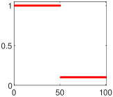
|
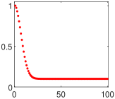
|
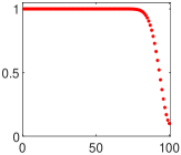
|
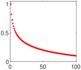
|
| (a) | (b) | (c) | (d) |
17.4. The randomized Kaczmarz method and its relatives
The Kaczmarz method is an iterative algorithm for solving linear systems that is typically used for large, overdetermined problems with inconsistent equations. Randomized variants of the Kaczmarz method have received a lot of attention in recent years, in part because of close connections to stochastic gradient descent (SGD) algorithms for solving least-squares problems.
To explain the idea, consider a (possibly inconsistent) linear system
| (17.4) |
The basic Kaczmarz algorithm starts with an initial guess for the solution. At each iteration , we select a new index , and we make the update
| (17.5) |
The rule (17.5) has a simple interpretation: it ensures that is the closest point to in the hyperplane containing solutions to the linear equation determined by the th equation in the system.
In implementing this method, we must choose a control mechanism that determines the next index. A simple and robust approach is to cycle through the rows consecutively; that is, . Another effective, but expensive, option is to select the equation with the largest violation.
The randomized Kaczmarz (RK) algorithm uses a probabilistic control mechanism instead. This kind of approach also has a long history, and it is useful in cases where cyclic control is ineffective. The RK method has received renewed attention owing to work of ?. They proposed sampling each independently at random, with the probability of choosing the th equation proportional to the squared norm of the th column of . They proved that this version of RK converges linearly with a rate determined by the (Demmel) condition number of the matrix . Later, it was recognized that this approach is just a particular instantiation of SGD for the least-squares problem (17.4). See ?, which draws on results from ?.
There are many subsequent papers that have built on the RK approach for solving inconsistent linear systems. ? observed that related ideas can be used to design randomized Gauss–Seidel and randomized Jacobi iterations. ? studied a blocked version of the RK algorithm, which is practically more efficient for many of the same reasons that other blocked algorithms work well (Section 16.2).
? observed that the RK algorithm is a particular type of iterative sketching method. Based on this connection, they proposed a generalization. At each iteration, we draw an independent random embedding . The next iterate is chosen by solving the least-squares problem
| (17.6) |
The idea is to choose the dimension sufficiently small that the sketched least-squares problem can be solved explicitly using a direct method (e.g., QR factorization). This flexibility leads to algorithms that converge more rapidly in practice because the sketch can mix equations instead of just sampling. Later, ? showed that this procedure can be accelerated to achieve rates that depend on the square root of an appropriate condition number; see also ?.
18. Linear solvers for graph Laplacians
In this section we describe the randomized algorithm, SparseCholesky, which can efficiently solve a linear system whose coefficient matrix is a graph Laplacian matrix. Up to a polylogarithmic factor, this method achieves the minimum possible runtime and storage costs. This algorithm has the potential to accelerate many types of computations involving graph Laplacian matrices.
The SparseCholesky algorithm was developed by ? and further refined by ?. These approaches are based on earlier work from Dan Spielman’s group, notably the paper of ?. The presentation here is adapted from ?.
18.1. Overview
We begin with a high-level approach for solving Laplacian linear systems. The basic idea is to construct a preconditioner using a randomized variant of the incomplete Cholesky method. Then we can solve the original linear system by means of the preconditioned conjugate gradient (PCG) algorithm.
18.1.1. Approximate solutions to the Poisson problem
Let be the Laplacian matrix of a weighted, loop-free, undirected graph on the vertex set . We write for the number of edges in the graph, i.e., the sparsity of the graph. For simplicity, we will also assume that the graph is connected; equivalently, where is the vector of ones. See Section 7.4 for definitions. See Figure 8 for an illustration of an unweighted, undirected graph.
The basic goal is to find the unique solution to the Poisson problem
For a parameter , we can relax this requirement by asking instead for an approximate solution that satisfies
We have written for the energy seminorm induced by the Laplacian matrix.
18.1.2. Approximate Cholesky decomposition
Imagine that we can efficiently construct a sparse, approximate Cholesky decomposition of the Laplacian matrix . More precisely, we seek a morally lower-triangular matrix that satisfies
| (18.1) |
In other words, there is a known permutation of the rows that brings the matrix into lower-triangular form. As usual, is the semidefinite order, and nnz returns the number of nonzero entries in a matrix.
This section describes an algorithm, called SparseCholesky, that can complete the task outlined in the previous paragraph. This algorithm is motivated by the insight that we can produce a sparse approximation of a Laplacian matrix by random sampling (Section 7.4). The main challenge is to obtain sampling probabilities without extra computation. The resulting method can be viewed as a randomized variant of the incomplete Cholesky factorization (?, Sec. 11.5.8).
18.1.3. Preconditioning
Given the sparse, approximate Cholesky factor , we can precondition the Poisson problem:
| (18.2) |
When (18.1) holds, the matrix has condition number .
Therefore, we can solve the preconditioned system (18.2) quickly using the PCG algorithm (?, Sec. 11.5). If the initial iterate , then steps of PCG produce an iterate that satisfies
As a consequence, we can achieve relative error after iterations. Each iteration requires a matrix–vector product with and the solution of a (consistent) linear system . We can perform these steps in operations per iteration. Indeed, has only nonzero entries. The matrix is morally triangular with nonzero entries, so we can apply using two triangular solves.
Remark 18.1 (Triangular solve).
To solve a consistent linear system , we can apply by triangular elimination and then apply by triangular elimination. The four subspace theorem ensures that solution to the first problem renders the second problem consistent too. Since , we can enforce consistency numerically by removing the constant component of the input . Similarly, we can remove the constant component of the output to ensure it belongs to the correct space.
18.1.4. Main results
The following theorem describes the performance of the SparseCholesky procedure. This is the main result from ?.
Theorem 18.2 (SparseCholesky).
Let be the Laplacian of a connected graph on vertices, with weighted edges. With high probability, the SparseCholesky algorithm produces a morally lower-triangular matrix that satisfies
The matrix has nonzero entries. The expected running time is operations.
In view of our discussion about PCG, we arrive at the following statement about solving the Poisson problem.
Corollary 18.3 (Poisson problem).
Suppose the SparseCholesky algorithm delivers an approximation that satisfies (18.1). Then we can solve each consistent linear system to relative error in the seminorm using at most iterations of PCG, each with a cost of arithmetic operations.
18.1.5. Discussion
As we have mentioned, the Poisson problem serves as a primitive for undertaking many computations on undirected graphs (?). Potential applications include clustering, analysis of random walks, and finite-element discretizations of elliptic PDEs.
The SparseCholesky algorithm achieves a near-optimal runtime and storage guarantee for the Poisson problem on a graph. Indeed, for a general graph with edges, any algorithm must use storage and arithmetic. There is a proof that the cost is achievable in theory (?), but the resulting methods are currently impractical. Meanwhile, the simplicity of the SparseCholesky method makes it a candidate for real-world computation.
For particular classes of Laplacian matrices, existing solvers can be very efficient. Optimized sparse direct solvers (?) work very well for small- and medium-size problems, but they typically have superlinear scaling, which renders them unsuitable for truly large-scale problems. Iterative methods such as multigrid or preconditioned Krylov solvers can attain linear complexity for important classes of problems, in particular for sparse systems arising from the discretization of elliptic PDEs. However, we are not aware of competing methods that provably enjoy near-optimal complexity for all problems.
We regard the SparseCholesky algorithm as one of the most dramatic examples of how randomization has the potential to accelerate basic linear algebra computations, both in theory and in practice.
18.2. Cholesky decomposition of a graph Laplacian
To begin our explanation of the SparseCholesky algorithm, let us summarize what happens when we apply the standard Cholesky decomposition method to a graph Laplacian.
18.2.1. The Laplacian of a multigraph
For technical reasons, related to the design and analysis of the algorithm, we need to work with multigraphs instead of ordinary graphs. In the discussion, we will point out specific places where this generality is important.
Consider a weighted, undirected multigraph , defined on the vertex set . Each edge is an unordered pair of vertices; we typically use the abbreviated notation . We introduce a weight function that assigns a positive weight to each edge in the multigraph . Since is a multigraph, there may be many multiedges, with distinct weights, connecting the same two vertices.
Taking some notational liberties, we will identify the multigraph with its Laplacian matrix , which we express in the form
| (18.3) |
The matrix is the elementary Laplacian on the vertex pair that composes the edge . That is,
The sum in (18.3) takes place over all the multiedges in the multigraph , so the same elementary Laplacian may appear multiple times with different weights.
18.2.2. Stars and cliques
To describe the Cholesky algorithm on a graph, we need to introduce a few more concepts from graph theory. Define the degree and the total weight of a vertex in the multigraph to be
In other words, the degree of is the total number of multiedges that contain . The total weight of is the sum of the weights of the multiedges that contain .
Let be a fixed vertex. The star induced by is the Laplacian
In words, the star includes precisely those multiedges in the multigraph that contain the vertex .
The clique induced by is defined implicitly as the correction that occurs when we take the Schur complement (2.4) of the Laplacian with respect to the coordinate :
Recall that is the standard basis vector in coordinate . By direct calculation, one may verify that
Each sum takes place over all multiedges in that contain the vertex . It can be verified that the clique is also the Laplacian of a weighted multigraph.
Figures 8 and 9 contain an illustration of a (simple) graph, along with the star and clique induced by eliminating a vertex. In our more general setting, the edges in the star and clique would have associated weights. These diagrams are courtesy of Richard Kueng.
18.2.3. Graphs and Cholesky
With the notation introduced in Section 18.2.2, we can present the graph-theoretic interpretation of the Cholesky algorithm as it applies to the Laplacian of a weighted multigraph.
Define the initial Laplacian . In each step , we select a new vertex . We extract the associated column of the current Laplacian:
We compute the Schur complement with respect to the vertex :
In other words, we remove the star induced by and replace it with the clique induced by . Each is the Laplacian of a multigraph; it has no multiedge that contains any one of the vertices . Therefore, we have reduced the size of the problem.
After steps, the Cholesky factorization is determined by a vector that holds the chosen indices and a matrix such that is lower-triangular. The algorithm ensures that we have the exact decomposition
This is the (pivoted) Cholesky factorization of the Laplacian matrix.
To choose a vertex to eliminate, the classical approach is to find a vertex with minimum degree or with minimum total weight. Or one may simply select one of the remaining vertices at random.
18.2.4. Computational costs
The cost to compute a Cholesky factorization of a Laplacian matrix is typically superlinear in , with a worst-case cost of arithmetic and storage. This is the reason that is less sparse than : the clique that is introduced at an elimination step has more edges than the star that it replaces, a phenomenon referred to as fill-in. The exact growth in the number of nonzero entries depends on the sparsity pattern of and on the chosen elimination order. For special cases, using a nested dissection ordering can provably improve on the worst-case estimates (?). For instance, if results from the finite-difference or finite-element discretization of an elliptic PDE, then in two dimensions and in three.
For general graphs, one path towards improving the efficiency of the Cholesky factorization procedure is to randomly approximate the clique by sampling, in order to curb the fill-in. Section 7.4 already indicates that this innovation may be possible, provided that we can find a way to obtain sampling probabilities.
18.3. The SparseCholesky algorithm
We are now prepared to present the SparseCholesky procedure, which uses randomized sampling to compute a sparse, approximate Cholesky factorization.
18.3.1. Procedure
Let be the Laplacian of a weighted multigraph on . We perform the following steps.
-
(1)
Preprocessing. Split each multiedge in into multiedges, each connecting , and each with weight . The purpose of this step is to control the effective resistance (7.5) of each multiedge at the outset of the algorithm. Note that this splitting results in a weighted multigraph, even if we begin with a simple graph.
-
(2)
Initialization. Form the initial Laplacian and the list of remaining vertices .
-
(3)
Iteration. For each :
-
(a)
Select a vertex. Choose a vertex uniformly at random from . Remove this vertex from the list: .
-
(b)
Extract the column. Copy the normalized th column from the current Laplacian:
Set if the denominator equals zero.
-
(c)
Sampling the clique. Construct the Laplacian of a random sparse approximation of . We will detail this procedure in Section 18.3.2.
-
(d)
Approximate Schur complement. Form
-
(a)
-
(4)
Decomposition. Collate the columns into the Cholesky factor
Define the row permutation for each .
Once these operations are complete, is a sparse, morally lower-triangular matrix. It is also very likely that . Theorem 18.2 makes a rigorous accounting of these claims.
18.3.2. Clique sampling
The remaining question is how to construct a random approximation of a clique . Here is the procedure:
-
(1)
Probabilities. Construct a probability mass such that
-
(2)
Sampling. For each ,
-
(a)
Draw a random multiedge from the multiedges in according to the probability mass .
-
(b)
Draw a second random multiedge from the multiedges in according to the uniform distribution.
-
(c)
Form the random Laplacian matrix of a new multiedge:
-
(a)
-
(3)
Approximation. Return .
The key fact about this construction is that it produces an unbiased estimator of the clique:
Furthermore, each summand creates a multiedge with uniformly bounded effective resistance (7.5). This property persists as the SparseCholesky algorithm executes, and it ensures that the random matrix has controlled variance. Note that the sampling procedure can result in several edges between the same pair of vertices, which is another reason we need the multigraph formalism.
Next, observe that the number of multiedges in is no greater than the number of multiedges in the star that we are removing from . (For comparison, note that the full clique has multiedges.) As a consequence, the clique approximation is inexpensive to construct. Moreover, the total number of multiedges in the Laplacian can only decrease as the SparseCholesky algorithm proceeds.
18.3.3. Analysis
The analysis of SparseCholesky is well beyond the scope of this paper. The key technical tool is a concentration inequality for matrix-valued martingales that was derived in (?) and (?). To activate this result, (?) use the fact that the random clique approximation is unbiased and low-variance, conditional on previous choices made by the algorithm. The proof also relies heavily on the fact that we eliminate a random vertex at each step of the iteration. For the technical details, see (?, ?) and (?).
18.3.4. Implementation
The SparseCholesky algorithm is fairly simple to describe, but it demands some care to develop an implementation that achieves the runtime guarantees stated in Theorem 18.2.
The most important point is that we need to use data structures for weighted multigraphs. One method is to maintain the vertex–multiedge adjacency matrix, along with a list of weights. This approach requires sparse matrix libraries, including efficient iterators over the rows and columns.
A secondary point is that we need fast methods for constructing finite probability distributions and sampling from them repeatedly. See ?.
It is unlikely that the SparseCholesky procedure will fail to produce a factor that satisfies (18.1). Even so, it is reassuring to know that we can detect failures. Indeed, we can estimate the extreme singular values of the preconditioned linear system (18.2) using the methods from Section 6.
The failure probability can also be reduced by modifying the random vertex selection rule. Instead, we can draw a random vertex whose total weight is at most twice the average total weight of the remaining vertices (?). In practice, it may suffice to use the classical elimination rules based on minimum degree or minimum total weight.
The main shortcoming of the SparseCholesky procedure arises from the initialization step, where we split each multiedge into pieces. This step increases the storage and computation costs of the algorithm enough to make it uncompetitive (e.g. with fast direct Poisson solvers) for some problem instances. At present, it is unclear whether the initialization step can be omitted or relaxed, while maintaining the reliability and correctness of the algorithm.
19. Kernel matrices in machine learning
Randomized NLA algorithms have played a major role in developing scalable kernel methods for large-scale machine learning. This section contains a brief introduction to kernels. Then it treats two probabilistic techniques that have had an impact on kernel matrix computations: Nyström approximation by random coordinate sampling (?) and empirical approximation by random features (?).
The literature on kernel methods is truly vast, so we cannot hope to achieve comprehensive coverage within our survey. There are also many computational considerations and learning-theoretic aspects that fall outside the realm of NLA. Our goal is simply to give a taste of the ideas, along with a small selection of key references.
19.1. Kernels in machine learning
We commence with a crash course on kernels and their applications in machine learning. The reader may refer to ? for a more complete treatment.
19.1.1. Kernel functions and kernel matrices
Let be a set, called the input space or data space. Suppose that we acquire a finite set of observations . We would like to use the observed data to perform learning tasks.
One approach is to introduce a kernel function:
The value of the kernel function is interpreted as a measure of similarity between two data points and . We can tabulate the pairwise similarities of the observed data points in a kernel matrix:
The kernel matrix is an analog of the Gram matrix of a set of vectors in a Euclidean space. In Sections 19.1.5 and 19.1.6, we will explain how to use the matrix to solve some core problems in data analysis.
The kernel function is required to be positive definite. That is, for each natural number and each set of observations, the associated kernel matrix
In particular, for all . The kernel must also be (conjugate) symmetric in its arguments: for all . These properties mirror the properties of a Gram matrix. In Section 19.1.3, we give some examples of positive definite kernel functions.
19.1.2. The feature space
It is common to present kernel functions using the theory of reproducing kernel Hilbert spaces. This approach gives an alternative interpretation of the kernel function as the inner product defined on a feature space. We give a very brief treatment, omitting all technical details.
Let be a Hilbert space, called the feature space. We introduce a feature map , which maps a point in the input space to a point in the feature space. Heuristically, the feature map extracts information from a data point that is relevant for learning applications.
Under mild conditions, we can construct a positive definite kernel function from the feature map:
In other words, the kernel function reports the inner product between the features associated with the data points and . Conversely, a positive definite kernel always induces a feature map into an appropriate feature space.
19.1.3. Examples of kernels
Kernel methods are powerful because we can select or design a kernel that automatically extracts relevant feature information from our data. This approach applies in all sorts of domains, including images and text and DNA sequences. Let us present a few kernels that commonly arise in applications. See ? for many additional examples and references.
Example 19.1 (Inner product kernel).
The simplest example of a kernel is the ordinary inner product. Let . Evidently,
is a positive definite kernel.
Example 19.2 (Angular similarity).
Another simple example is the angular similarity map. Let . This kernel is given by the formula
This kernel is positive definite because of Schoenberg’s theorem (?). We will give a short direct proof in Example 19.8.
Example 19.3 (Polynomial kernels).
Let be a subset of . For a natural number , the inhomogeneous polynomial kernel is
This kernel is also positive definite because of Schoenberg’s theorem; see ?. There is a short direct proof using the Schur product theorem.
Example 19.4 (Gaussian kernel).
An important example is the Gaussian kernel. Let . For a bandwidth parameter , define
This kernel is positive definite because of Bochner’s theorem (?). We will give a short direct proof in Example 19.9.
19.1.4. The kernel trick
As we have mentioned, kernels can be used for a wide range of tasks in machine learning. ? state the key idea succinctly:
Given an algorithm which is formulated in terms of a positive definite kernel , one can construct an alternative algorithm by replacing with another positive definite kernel .
In particular, any algorithm that can be formulated in terms of the inner product kernel applies to every other kernel. That is to say, an algorithm for Euclidean data that depends only on the Gram matrix can be implemented with a kernel matrix instead. The next two subsections give two specific examples of this methodology; there are many other applications.
19.1.5. Kernel PCA
Given a set of observations in a Euclidean space, principal component analysis (PCA) searches for orthogonal directions in which the data has the maximum variability. The nonlinear extension, kernel PCA (KPCA), was proposed in ?; see also ?.
Let be a set of observations. For a kernel associated with a feature map , construct the kernel matrix associated with the observations. For a natural number , we compute a truncated eigenvalue decomposition of the kernel matrix:
Each unit-norm eigenvector determines a direction of high variability in the feature space, called the th kernel principal component.
To find the projection of a new point onto the th kernel principal component, we embed it into the feature space via and compute the inner product with the th kernel principal component. In terms of the kernel function,
We can summarize the observation with the vector
This representation provides a data-driven feature that can be used for downstream learning tasks.
In practice, it is valuable to center the feature space representation of the data, which requires a simple modification of the kernel matrix. We also need to center each observation before computing its projection onto the kernel principal components. See ? for details.
19.1.6. Kernel ridge regression
Given a set of labeled observations in a Euclidean space, ridge regression uses regularized least-squares to model the labels as a linear functional of the observations. The nonlinear extension of this approach is called kernel ridge regression (KRR). We refer to ? for a more detailed treatment, including an interpretation in terms of a nonlinear feature map.
Let be a set of paired observations. For a kernel , construct the kernel matrix associated with the observations (but not the numerical values ). For a regularization parameter , the kernel ridge regression problem takes the form
The solution to this optimization problem is obtained by solving an ordinary linear system:
Let be the solution to this system.
Given a new observation , we can make a prediction for its label via the formula
In practice, the regularization parameter is chosen by cross-validation with a holdout set of the paired observations.
19.1.7. The issue
Kernel methods are powerful tools for data analysis. Nevertheless, in their native form, they suffer from two weaknesses.
First, it is very expensive to compute the kernel matrix explicitly. For example, if points in the data space have a -dimensional parameterization, we may expect that it will cost arithmetic operations to evaluate the kernel a single time. Therefore, the cost of forming the kernel matrix for observations is .
Second, after computing the kernel matrix , it remains expensive to perform the linear algebra required by kernel methods. Both KPCA and KRR require operations if we use direct methods.
The poor computational profile of kernel methods limits our ability to use them directly for large-scale data applications.
19.1.8. The solution
Fortunately, there is a path forward. To implement kernel methods, we simply need to approximate the kernel matrix (?, Sec. 10.2). Surprisingly, using the approximation often results in better learning outcomes than using the exact kernel matrix. Even a poor approximation of the kernel can suffice to achieve near-optimal performance, both in theory and in practice (?, ?, ?). Last, working with a structured approximation of the kernel can accelerate the linear algebra computations dramatically.
Randomized algorithms provide several effective tools for approximating kernel matrices. Since we pay a steep price for each kernel evaluation, we need to develop algorithms that explicitly control this cost. The rest of this section describes two independent approaches. In Section 19.2, we present coordinate sampling algorithms for Nyström approximations, while Section 19.3 develops the method of random features.
Remark 19.5 (Function approximation).
Let us remark that approximation of the kernel matrix is usually incidental to the goals of learning theory. In many applications, such as KRR, we actually need to approximate a function on the input space. The sampling complexity of the latter task may be strictly lower than the complexity of approximating the full kernel matrix. We cannot discuss this issue in detail because it falls outside the scope of NLA.
19.2. Coordinate Nyström approximation of kernel matrices
One way to approximate a kernel matrix is to form a Nyström decomposition with respect to a judiciously chosen coordinate subspace. A natural idea is to draw these coordinates at random. This basic technique was proposed by ?.
Coordinates play a key role here because we only have access to individual entries of the kernel matrix. There is no direct way to compute a matrix–vector product with the kernel matrix, so we cannot easily apply the more effective constructions of random embeddings (e.g., Gaussians or sparse maps or SRTTs). Indeed, kernel computation is the primary setting where coordinate sampling is a practical idea.
19.2.1. Coordinate Nyström approximation
Suppose that is a collection of observations. Let be the psd kernel matrix associated with some kernel function .
Given a set consisting of indices, we can form a psd Nyström approximation of the kernel matrix:
This matrix is equivalent to the Nyström decomposition (14.1) with respect to a test matrix whose range is .
To obtain , the basic cost is kernel evaluations, which typically require operations for a -dimensional input space . We typically do not form the pseudoinverse directly, but rather use the factored form of the Nyström approximation for downstream calculations.
For kernel problems, it is common to regularize the coordinate Nyström approximation. One approach replaces the core matrix with its truncated eigenvalue decomposition before computing the pseudoinverse; for example, see ?. The RSVD algorithm (Section 11.2) has been proposed for this purpose (?). When it is computationally feasible, we recommend taking a truncated eigenvalue decomposition of the full Nyström approximation , rather than just the core; see ?.
19.2.2. Greedy selection of coordinates
Recall from Section 14 that the error in the Nyström decomposition is simply the Schur complement of with respect to the coordinates in .
This connection suggests that we should use a pivoted Cholesky method or a pivoted QR algorithm to select the coordinates . These techniques lead to Nyström approximations with superior learning performance; for example, see (?, ?) and (?). Unfortunately the cost is prohibitive in applications. See ? for some randomized strategies that can reduce the expense.
19.2.3. Ridge leverage scores
A natural approach to selecting the coordinate set is to perform randomized sampling. To describe these approaches, we need to take a short detour.
Fix a regularization parameter . Consider the smoothed projector:
The number of effective degrees of freedom at regularization level is
The maximum marginal number of degrees of freedom at regularization level is
Observe that . The statistic is analogous with the coherence that appears in our initial discussion of coordinate sampling (Section 9.6).
The ridge leverage scores at regularization level are the (normalized) diagonal entries of the smoothed projector:
Evidently, is a probability distribution. The ridge leverage scores and related quantities are expensive to compute directly, but there are efficient algorithms for approximating them well. These approximations suffice for applications. See Section 19.2.5 for more discussion.
Remark 19.6 (History).
? identified the core role of the smoothed projector for KRR. ? proposed the definition of the ridge leverage scores and described a simple method for approximating them. At present, the most practical algorithm for approximating ridge leverage scores appears in ?. ? recognize that ridge leverage scores also have relevance for KPCA.
19.2.4. Uniform sampling
The simplest way to select a set of coordinates for the Nyström approximation is to draw the set uniformly at random. Although this approach seems naïve, it can be surprisingly effective in practice. The main failure mode occurs when there are a few significant observations that make outsize contributions to the kernel matrix; uniform sampling is likely to miss these influential data points.
? proves that we can achieve optimal learning guarantees for KRR with a uniformly sampled Nyström approximation. It suffices that the number of coordinates is proportional to . A similar result holds for KPCA.
Nyström approximation with uniform coordinate sampling was proposed by ?. The theoretical and numerical performance of this approach has been studied in many subsequent works, including (?, ?, ?) and (?).
19.2.5. Sampling with ridge leverage scores
Suppose that we have computed an approximation of the ridge leverage score distribution. We can construct a coordinate set for the Nyström approximation by sampling coordinates independently at random from the ridge leverage score distribution. Properly implemented, this method is unlikely to miss influential observations.
? prove that we can achieve optimal learning guarantees for KRR by ridge leverage score sampling. It suffices that the number of sampled coordinates is proportional to . This bound improves over the uniform sampling bound. ? give related theoretical results for KPCA.
Effective algorithms for estimating ridge leverage scores are based on multilevel procedures that sequentially improve the ridge leverage score estimates. The basic idea is to start with a small uniform sample of coordinates, which we use to approximate the smoothed projector for a very large regularization parameter . From this smoothed projector, we estimate the ridge leverage scores at level . We then sample a larger set of coordinates non-uniformly using the approximate ridge leverage score distribution at level . These samples allow us to approximate the smoothed projector at level for a constant smaller than one. We obtain an estimate for the ridge leverage score distribution at level . This process is repeated. In this way, the sampling and the matrix approximation are intertwined. See (?) and (?).
? provide empirical evidence that ridge leverage score sampling is more efficient than uniform sampling for KPCA, including the cost of the ridge leverage score approximations. Likewise, ? report empirical evidence that ridge leverage score sampling is more efficient than uniform sampling for KRR.
19.3. Random features approximation of kernels
A second approach to kernel approximation is based on the method of empirical approximation (Section 7). This technique constructs a random rank-one matrix that serves as an unbiased estimator for the kernel matrix. By averaging many copies of the estimator, we can obtain superior approximations of the kernel matrix. The individual rank-one components are called random features.
? proposed the idea of using empirical approximation for kernels arising in Gaussian process regression. Later, ? and ? developed empirical approximations for translation-invariant kernels and Mercer kernels, and they coined the term “random features.” Our presentation is based on an abstract formulation of the random feature method from ?; see also ?.
In this subsection, we introduce the idea of a random feature map, along with some basic examples. We explain how to use random feature maps to construct empirical approximations of a kernel matrix, and we give a short analysis. Afterwards, we summarize two randomized NLA methods for improving the computational profile of random features.
19.3.1. Random feature maps
In many cases, a kernel function on a domain can be written as an expectation, and we can exploit this representation to obtain empirical approximations of the kernel matrix.
Let be a probability space equipped with a probability measure . Assume that there is a bounded function
with the reproducing property
| (19.1) |
The star ∗ denotes the conjugate of a complex number. We call a random feature map for the kernel function . As we will see in Section 19.3.2, a kernel that admits a random feature map must be positive definite.
It is not obvious that we can equip kernels of practical interest with random feature maps, so let us offer a few concrete examples.
Example 19.7 (The inner product kernel).
There are many ways to construct a random feature map for the inner product kernel on . One simple example is
To check that this map satisfies the reproducing property (19.1), just note that is isotropic: . This formulation is closely related to the theory of random embeddings (Sections 8 and 9) and to approximate matrix multiplication (Section 7.3).
Example 19.8 (Angular similarity kernel).
For the angular similarity map defined in Example 19.2, we can construct a random feature map using an elegant fact from geometry. Indeed, the function
gives a random feature map for the angular similarity kernel. As a consequence, the angular similarity kernel is positive definite.
Example 19.9 (Translation-invariant kernels).
A kernel function on is called translation-invariant if it has the form
A classic result from analysis, Bochner’s theorem (?), gives a characterization of these kernels. A kernel is continuous, positive definite and translation-invariant if and only if it is the Fourier transform of a positive probability measure on :
The constant is a normalizing factor that depends only on , and is the imaginary unit.
Bochner’s theorem immediately delivers a random feature map for the translation-invariant kernel :
This was one of the original examples of a random feature map (?). When working with data in , the construction can also be modified to avoid complex values.
The key example of a positive definite, translation-invariant kernel is the Gaussian kernel on , defined in Example 19.4. The Gaussian kernel is derived from the function
The associated random feature map is
This fact is both beautiful and useful because of the ubiquity of the Gaussian kernel in data analysis.
There are many other kinds of kernels that admit random feature maps. Random feature maps for dot product kernels were obtained in (?, ?) and (?). For nonstationary kernels, see (?) and (?). Catalogs of examples appear in ? and ?.
19.3.2. Random features and kernel matrix approximation
We can use the random feature map to construct an empirical approximation of the kernel matrix induced by the dataset . To do so, we draw a random variable with the distribution . Then we form a random vector
Note that we are using the same random variable for each data point. A realization of the random vector is called a random feature. The reproducing property (19.1) ensures that the random feature verifies the identity
In matrix form,
Therefore, the random rank-one psd matrix is an unbiased estimator for the kernel matrix. The latter display proves that a kernel must be positive definite if it admits a random feature map.
To approximate the kernel matrix, we can average copies of the rank-one estimator:
If the points in the input space are parameterized by numbers, each random feature typically requires arithmetic. The total cost of forming the approximation is thus . When , we can obtain substantial improvements over the direct approach of computing the kernel matrix explicitly at a cost of .
19.3.3. Analysis of the random feature approximation
How many random features are enough to approximate the kernel matrix in spectral norm? Theorem 7.2 delivers bounds.
For simplicity, assume that the kernel satisfies for all ; the angular similarity kernel and the Gaussian kernel both enjoy this property. For an accuracy parameter , suppose that we select
The number is the uniform bound on the feature map defined in (19.1), and the intrinsic dimension is defined in (2.1). Theorem 7.2 implies that the empirical approximation satisfies
In other words, we achieve a relative error approximation of the kernel matrix in spectral norm when the number of random features is proportional to the number of energetic dimensions in the range of the matrix .
This analysis is due to ?; see also (?, Sec. 6.5). For learning applications, such as KPCA or KRR, this result suggests that we need about random features to obtain optimal generalization guarantees (where ). In fact, roughly random features are sufficient to achieve optimal learning rates. This claim depends on involved arguments from learning theory that are outside the realm of linear algebra. For example, see (?, ?, ?, ?) and (?).
19.3.4. Randomized embeddings and random features
Random feature approximations are faster than explicit computation of a kernel matrix. Even so, it takes a significant amount of effort to extract random features and form an empirical approximation of the kernel matrix. Several groups have proposed using structured random embeddings (Section 9) to accelerate this process; see (?, ?) and (?).
As an example, let us summarize a heuristic method, called FFT Fastfood (?), for speeding up the computation of random features for the complex Gaussian kernel with bandwidth . Consider the matrix formed from observations in :
Let be a matrix with iid complex entries. Then we can simultaneously compute random features for the Gaussian kernel by forming a matrix product and applying the exponential map:
We have written for the entrywise exponential. This procedure typically involves arithmetic.
The idea behind FFT Fastfood is to accelerate this computation by replacing the Gaussian matrix with a structured random matrix. This exchange is motivated by the observed universality properties of random embeddings. Consider a random matrix of the form
where is a random sign flip, is a random permutation, and is the discrete DFT. The FFT algorithm supports efficient matrix products with . Therefore, we can simultaneously extract random features by computing . This procedure uses only operations. To form random features where , we simply repeat the same process times.
Compared with using a Gaussian matrix product, FFT Fastfood gives a substantial reduction in arithmetic. Even so, the performance for learning is almost identical to a direct application of the random feature approximation.
19.3.5. Random features and streaming matrix approximation
Suppose that we wish to perform KPCA. The direct random features approach requires us to form the empirical approximation of the kernel matrix and to compute its rank- truncated eigenvalue decomposition. It is often the case that the desired number of principal components is far smaller than the number of random features we need to obtain a suitable approximation of the kernel matrix. In this case, we can combine random features with streaming matrix approximation to make economies in storage and computation.
Let be an iid sequence of random features for the kernel matrix . The empirical approximation of the kernel matrix, obtained from the first random features, follows the recursion
This is a psd matrix, generated by a stream of linear updates. Therefore, we can track the evolution using a streaming Nyström approximation (Section 14).
Let be a random test matrix, with . By performing rank-one updates, we can efficiently maintain the sample matrices
After collecting a sufficient number of samples, we can apply Algorithm 16 to to obtain a near-optimal rank- eigenvalue decomposition of the empirical approximation .
It usually suffices to take the sketch size to be proportional to the rank of the truncated eigenvalue decomposition. In this case, the overall approach uses storage. We can generate and process random features using arithmetic, where is the dimension of . The subsequent cost of the Nyström approximation is operations. The streaming random features approach has storage and arithmetic costs roughly times those of the direct random features approach. The streaming method can be combined with dimension reduction techniques (Section 19.3.4) for further acceleration.
Remark 19.10 (History).
? proposed using a stream of random features to perform KPCA; their algorithm tracks the stream with the (deterministic) frequent directions sketch (?). We have presented a new variant, based on randomized Nyström approximation, that is motivated by the work in ?. ? have develop a somewhat different streaming KPCA algorithm based on Oja’s method (?). At present, we lack a full empirical comparison of these alternatives.
20. High-accuracy approximation of kernel matrices
In this section, we continue the discussion of kernel matrices that we started in Section 19, but we now consider the high-accuracy regime. In particular, given a kernel matrix , we seek an approximation for which is small, say of relative accuracy or . This objective was not realistic for the applications discussed in Section 19, but it can be achieved in situations where we have access to fast techniques for evaluating the matrix-vector product (and also when is not self-adjoint). The algorithms that we describe will build a data sparse approximation to by using information in samples such as and for random vectors . These techniques are particularly well suited to problems that arise in modeling physical phenomena such as electromagnetic scattering, or the deformation of solid bodies; we describe how the fast matrix-vector application we need can be realized in Section 20.3.
As in Section 19, we say that a matrix is a kernel matrix if its entries are given by a formula such as
| (20.1) |
where is a set of points in , and where is a kernel function. The kernel matrices that we consider tend to have singular values that decay slowly or not at all, which rules out the possibility that could have low rank. Instead, we build an approximation that is tessellated into blocks in such as way that each off-diagonal block has low rank. Figure 11(b) shows a representative tessellation pattern. We say that a matrix of this type is a rank-structured hierarchical matrix.
The purpose of determining a rank-structured approximation to an operator for which we already have fast matrix-vector multiplication techniques available is that the new representation can be used to rapidly execute a whole range of linear algebraic operations: matrix inversion, LU factorization, and even full spectral decompositions in certain cases.
This section is structured to provide a high-level description of the core ideas in Sections 20.1 – 20.3. Additional details follow in Sections 20.4 – 20.9.
20.1. Separation of variables and low-rank approximation
The reason that many kernel matrices can be tessellated into blocks that have low numerical rank is that the function is typically smooth as long as and are not close. To illustrate the connection, let us consider a computational domain that holds a set of points , as shown in Figure 10. Suppose further that and are two subdomains of that are located a bit apart from each other, as shown in the figure. When the kernel function is smooth, we can typically approximate it to high accuracy through an approximate separation of variables of the form
| (20.2) |
Let and denote two index vectors that identify the points located in and , respectively (so that, for example, if and only if ). Then combining the formula (20.1) with the separation of variables (20.2), we get
| (20.3) |
Equation (20.3) is exactly the low-rank approximation to the block that we seek. To be precise, (20.3) can be written as
where and are defined via and .
A separation of variables such as (20.2) is sometimes provided through analytic knowledge of the kernel function, as illustrated in Example 20.1. Perhaps more typically, all we know is that such a formula should in principle exist, for instance because we know that the matrix approximates a singular integral operator for which a Calderón-Zygmund decomposition must exist. It is then the task of the randomized algorithm to explicitly build the factors and , given a computational tolerance.
Example 20.1 (Laplace kernel in two dimensions).
A standard example of a kernel matrix in mathematical physics is the matrix that maps a vector of electric source strengths to a vector of potentials . When the set identifies the locations of both the source and the target points, takes the form (20.1), for
There is a well-known result from potential theory that provides the required separation of variables. Expressing and in polar coordinates with respect to some expansion center , so that and , the separation of variables (known as a multipole expansion)
| (20.4) |
is valid whenever .
20.2. Rank-structured matrices and randomized compression
The observation that the off-diagonal blocks of a kernel matrix often have low numerical rank underpins many “fast” algorithms in computational physics. In particular, it is the foundation of the Barnes-Hut (?) and fast multipole methods (?) for evaluating all pairwise interactions between electrically charged particles in linear or close-to-linear complexity. These methods were generalized by Hackbusch and co-workers, who developed the - and -matrix frameworks (?, ?, ?). These explicitly linear algebraic formulations enable fast algorithms not only for matrix-vector multiplication but also for matrix inversion, LU factorization, matrix-matrix multiplication and many more.
A fundamental challenge that arises when rank-structured matrix formulations are used is how to find the data sparse representation of the operator in the first place. The straightforward approach would be to form the full matrix, and then loop over all the compressible off diagonal blocks and compress them using, for example, a singular value decomposition. The cost of such a process is necessarily at least , which is rarely affordable. Using randomized compression techniques, it turns out to be possible to compress all the off-diagonal blocks jointly, without any need for sampling each block individually. In this section, we describe two such methods. Both require the user to supply a fast algorithm for applying the full matrix (and its adjoint) to vectors; see Section 20.3. The two methods have different computational profiles.
-
(a)
The technique described in Sections 20.4 and 20.5 is a true “black-box” technique that interacts with only through the matrix-vector multiplication. It has storage complexity and it requires applications of to a random matrix of size where is an upper bound on the ranks of the off-diagonal blocks, and is a small over-sampling parameter.
-
(b)
The technique described in Sections 20.6 and 20.7 attains true linear complexity, and requires only a single application of and to a random matrix of size , where and are as in (a). Its drawbacks are that it requires evaluation of individual matrix entries, and that it works only for a smaller class of matrices.
Remark 20.2 (Scope of Section 20).
To keep the presentation as uncluttered by burdensome notation as possible, in this survey we restrict attention to two basic “formats” for representing a rank-structured hierarchical matrix. In Sections 20.4 and 20.5, we use the hierarchically off-diagonal low rank (HODLR) format and in Sections 20.6 and 20.7 we use the hierarchically block separable (HBS) format (sometimes referred to as hierarchically semi separable (HSS) matrices). The main limitation of these formats is that they require all off-diagonal blocks of the matrix to have low numerical rank. This is realistic only when the points are restricted to a low-dimensional manifold. In practical applications, one sometimes has to leave a larger part of the matrix uncompressed, to avoid attempting to impose a separation of variables such as (20.2) on a kernel when and are too close. This is done through enforcing what is called a “strong admissibility condition” (in contrast to the “weak admissibility condition” of the HODLR and HBS formats), as was done in the original Barnes-Hut and fast multipole methods.
Remark 20.3 (Alternative compression strategies).
Let us briefly describe what alternatives to randomized compression exist. The original papers on -matrices used Taylor approximations to derive a separation of variables, but this works only when the kernel is given analytically. It also tends to be quite expensive. The adaptive cross-approximation (ACA) technique of (?) and (?) relies on using “natural basis” vectors (see Section 13.1) that are found using semi-heuristic techniques. The method can work very well in practice, but is not guaranteed to provide an accurate factorization. When the kernel matrix comes from mathematical physics, specialized techniques that exploit mathematical properties of the kernel function often perform well (?). For a detailed discussion of compression of rank-structured matrices, we refer to (?, Ch. 17).
20.3. Computational environments
The compression techniques that we describe rely on the user providing a fast algorithm for applying the operator to be compressed to vectors. Representative environments where such fast algorithms are available include the following.
Matrix-matrix multiplication: Suppose that , where and are matrices that can rapidly be applied to vectors. Then the randomized compression techniques allow us to compute their product.
Compression of boundary integral operators: It is often possible to reformulate a boundary value problem involving an elliptic partial different operator, such as the Laplace or the Helmholtz operators, as an equivalent boundary integral equation (BIE), see (?, Part III). When such a BIE is discretized, the result is a kernel matrix which can be applied rapidly to vectors using fast summation techniques such as the fast multipole method (?). Randomized compression techniques allow us to build an approximation to the matrix that can be factorized or inverted, thus enabling direct (as opposed to iterative) solvers.
Dirichlet-to-Neumann (DtN) operators: A singular integral operator of central importance in engineering, physics, and scientific computing is the DtN operator which maps given Dirichlet data for an elliptic boundary value problem to the boundary fluxes of the corresponding solution. The kernel of the DtN operator is rarely known analytically, but the operator can be applied through a fast solver for the PDE, such as, e.g., a finite-element discretization combined with a multigrid solver. The randomized techniques described allow for the DtN operator to be built and stored explicitly.
Frontal matrices in sparse direct solvers: Suppose that is a large sparse matrix arising from the discretization of an elliptic PDEs. A common technique for solving is to compute an LU factorization of the matrix . There are ways to do this that preserve sparsity as far as possible, but in the course of the factorization procedure, certain dense matrices of increasing size will need to be factorized. These matrices turn out to be kernel matrices with kernels that are not known explicitly, but that can be built using the techniques described here (?, ?).
20.4. Hierarchically off-diagonal low-rank matrices
In order to illustrate how randomized methods can be used to construct data sparse representations of rank-structured matrices, we will describe a particularly simple ‘format’ in this section that is often referred to as the hierarchically off-diagonal low-rank (HODLR) format. This is a basic format that works well when the points are organized on a one- or two-dimensional manifold.
The first step towards defining the HODLR format is to build a binary tree on the index vector through a process that is illustrated in Figure 11(a). With any node in the tree, we associate an index vector . The root of the tree is given the index , and we associate it with the full index vector, so that . At the next finer level of the tree, we split into two parts and so that forms a disjoint partition. Then continue splitting the index vectors until each remaining index vector is “short”. (Exactly what “short” means is application-dependent, but one may think of a short vector as holding a few hundred indices or so.) We let denote a level of the tree, with denoting the root, so that level holds nodes. We use the terms parent and child in the obvious way, and say that a pair of nodes forms a sibling pair if they have the same parent. A leaf node is of course a node that has no children.
The binary tree that we defined induces a natural tessellation of the kernel matrix into blocks. Figure 11(b) shows the tessellation that follows from the tree in Figure 11(a). Each parent node in the tree gives rise to two off-diagonal blocks that both have low numerical rank. Letting denote the children of , these two blocks are
| (20.5) |
For each leaf node , we define a corresponding diagonal block as
| (20.6) |
The disjoint partition of into blocks is now formed by all sibling pairs, as defined in (20.5), together with all diagonal blocks, as defined by (20.6). When each off-diagonal block in this tessellation has low rank, we say that is a hierarchically off-diagonal low-rank (HODLR) matrix.
20.5. Compressing a rank-structured hierarchical matrix through the matrix-vector multiplication only
In this section, we describe a randomized technique for computing a data sparse representation of a matrix that is compressible in the “HODLR” format that we introduced in Section 20.4. This technique interacts with only through the application of and to vectors, and is in this sense a “black-box” technique. In particular, we do not need the ability to evaluate individual entries of . The following theorem summarizes the main result:
Theorem 20.4.
Let be a HODLR matrix associated with a fully populated binary tree on the index vector, as described in Section 20.4. Suppose that the tree has levels, that each off-diagonal block has rank at most , and that each leaf node in the tree holds at most indices for some fixed number . Then the diagonal blocks , as well as rank- factorizations of all sibling interaction matrices can be computed by a randomized algorithm with cost at most
where is the cost of applying either or to a vector, and is the cost of a floating point operation.
The proof of the theorem consists of an explicit algorithm for building all matrices that is often referred to as the “peeling algorithm”. It was originally published in (?), with later modifications proposed in (?). The proof below is based on (?, Sec. 17.4). We give the proof for the case described in the theorem involving a matrix whose off-diagonal blocks have exact rank . In practical applications, it is of course more typical to have the off-diagonal blocks be only of approximate low rank. In this case, the exact same algorithm can be used, but the number of samples drawn should be increased from to for some modest oversampling parameter .
Proof.
The algorithm is a “top-down” technique that compresses the largest blocks first, and then moves on to process one level at a time of successively smaller blocks. In describing the technique, we assume that the blocks are numbered as shown in Figure 11(a).
In the first step of the algorithm, we build approximations to the two largest blocks and , shown in red in Figure 12(a). To do this, we form a random matrix of size and then use the matrix-vector multiplication to form a sample matrix
The key idea of the peeling algorithm is to insert zero blocks in the random matrix in the pattern shown in Figure 12(a). The zero blocks permit us to extract “pure” samples from the column spaces of the blocks and . For instance, the blocks labeled and in the figure are given by the formulas
By orthonormalizing the matrices and , we obtain ON bases and for the off-diagonal blocks and . In order to complete the factorization of and , we will perform an operation that is the equivalent of “Stage B” in Section 11.2. To this end, we form a test matrix by interlacing the matrices and with zero blocks, to form the matrix shown in Figure 13. Applying to this test matrix, we get the sample matrices
Since holds an ON-basis for the column space of , it follows that
which establishes the low rank factorization of .222One may if desired continue the factorization process and form an “economy size” SVD of so that . This results in the factorization , which is an SVD of . However, for purposes of establishing the theorem, we may leave alone, and let be our “compressed” representation of . The block is of course factorized analogously.
| (a) In the first step of the algorithm, the sibling interaction matrices and on level 1, shown in red, are compressed. |
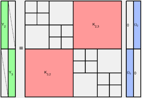
|
| (b) In the second step, the four sibling interaction matrices on level 2, shown in red, are compressed. In this step, we exploit that we now possess factorizations of the gray blocks. |
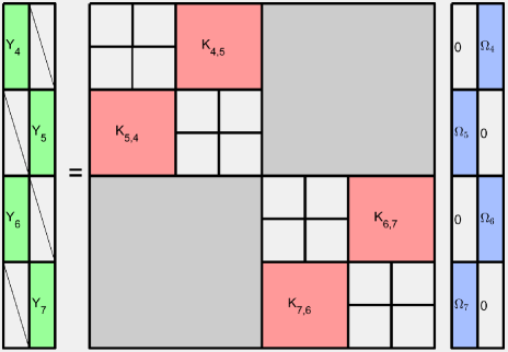
|
| (c) In the third step, the eight sibling interaction matrices on level 8, shown in red, are compressed. We again exploit that we possess factorizations of the gray blocks. |
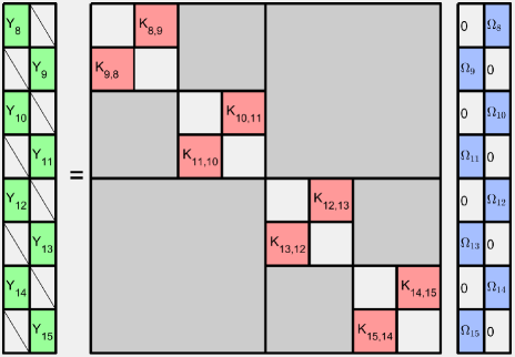
|
At the second step of the algorithm, the objective is to build approximations to the sibling matrices at the next finer level, shown in red in Figure 12(b). We use a random matrix of the same size, , as in the previous step, but now with four zero blocks, as shown in the figure. Looking at the sample matrix , we find that it takes the form
where represents contributions from interactions between the block and the random matrix and . But now observe that we at this point are in possession of a low rank approximation to . This allows us to compute explicitly, and then obtain a “pure” sample from the column space of by subtracting this contribution out:
By orthonormalizing the matrix , we obtain the ON matrix whose columns span the column space of . The same procedure of course also allows us to build bases for the column spaces of all matrices at this level, and we can then extract bases for the row spaces and the cores of the matrices by sampling .
At the third step of the algorithm, the object is to compress the blocks marked in red in Figure 12(c). The random matrix used remains of size but now contains 8 zero blocks, as shown in the figure. The sample matrix takes the form
where represents contributions from off-diagonal blocks at the coarser levels, shown in gray in the figure. Since we already possess data sparse representations of these blocks, we can subtract their contributions out, just as at the previous level.
Once all levels have been processed, we hold low-rank factorizations of all off-diagonal blocks, and all that remains is to extract the diagonal matrices for all leaf nodes . Let us for simplicity assume that all such block are of the same size . We then form a test matrix by stacking copies of an identity matrix atop of each other and applying to this test matrix. We subtract off the contributions from all the off-diagonal blocks using the representation we have on hand, and are then left with a sample matrix consisting of all the blocks stacked on top of each other. ∎
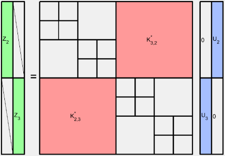
20.6. A linear complexity data sparse format
The “HODLR” data sparse matrix format discussed in Sections 20.4 and 20.5 is simple to use, and is in many applications efficient enough. However, its storage complexity is at least as the matrix size grows. We will next describe how the logarithmic factor can be eliminated. To keep the presentation concise, we focus on the asymptotic storage requirements, although similar estimates hold for the asymptotic flop count.
To start, let us first investigate why there are logarithmic factors in the storage requirement in the HODLR format. Suppose that for a sibling pair the corresponding off-diagonal block is of size , has rank , and is stored in the form of a factorization
where and are two matrices whose columns form bases for the column and row space of , respectively.333The matrices and were denoted and in Sections 20.4 and 20.5. We see that can be stored using about floating point numbers (where we ignore terms, since typically ). Now let us consider how many floats are required to store all sibling interaction matrices on a given level in the tree. There are such matrices, and they each have size , resulting in a total of floats. Since there are levels in the tree, it follows that just the task of storing all the basis matrices requires storage.
A standard technique for overcoming the problem of storing all the “long” basis matrices is to assume that the basis matrices on one level can be formed through slight modifications to the basis matrices on the next finer level. To be precise, we assume that if is a node in the tree with children and , then there exists a “short” basis matrix of size such that
| (20.7) |
(with of course an analogous statement holding for the “V” matrices holding bases for the row spaces). The point is that if we already have the “long” basis matrices for the children available, then the long basis matrices for the parent can be formed using the information in the small matrix . By applying this argument recursively, we see that for any parent node , all that needs to be stored explicitly are small matrices of size .
To illustrate the idea, suppose that we use this technique for storing basis matrices to the tree with three levels described in Section 20.4. Then for each of the 8 leaf boxes, we compute basis matrices of size and store these. At the next coarser level, the long basis matrix for a box such as can be expressed through the formula
so that only the matrix needs to be stored. At the next coarser level still, the long basis matrix is expressed as
We say that a matrix that can be represented using nested basis matrices in the manner described is a hierarchically block separable (HBS) matrix. (This format is very closely related to the hierarchically semi separable (HSS) matrix format described in (?, ?).) When the HBS format is used, it is natural to assume that each leaf index vector holds indices, which means that there are overall nodes in the tree. Since we only need storage per node, we see that the overall storage requirements improve from to .
There is a price to be paid for using “nested” basis matrices, and it is that the rank required to reach a requested precision typically is higher when nested basis matrices are used, in comparison to the HODLR format. To be precise, one can show that for the relation (20.7) to hold, it is necessary and sufficient that for a node , the columns of must span the column space of the matrix (where ). In contrast, in the HODLR format, they only need to span the columns of , where is the sibling of . This is easier to do since is a subset of the index vector .
20.7. A linear complexity randomized compression technique
We saw in Section 20.6 that the so called “HBS” data sparse format allows us to store a matrix using floating point numbers, without any factor of . But is it also possible to compute such a representation in optimal linear complexity? The answer is yes, and a number of deterministic techniques that work in specific environments have been proposed (?, Ch. 17). A linear complexity randomized technique was proposed in (?). This method is based on analyzing samples of the matrix obtained through the application of and to Gaussian random vectors, but is not quite a black-box method, as it also requires the ability to evaluate individual elements of itself. This is not always possible, of course, but when it is, the technique is lightning fast in practice. To be precise, (?) establishes the following:
Theorem 20.5.
Let be an matrix that is compressible in the HBS format described in Section 20.6, for some rank . Let denote the time it takes to evaluate the two products
| (20.8) | ||||
| (20.9) |
where is an matrix drawn from a Gaussian distribution. Then a full HBS representation of can be computed at cost bounded by
where is the cost of a floating point operation, and where is the time it takes to evaluate an individual entry of
When the off-diagonal blocks are only approximately of rank , we do some over sampling as usual, and replace the number in the theorem by for some small number . This of course results in an approximate HBS representation of .
The proof of Theorem 20.5 is an algorithm that explicitly builds the data sparse representation of the matrix within the specified time budget. The algorithm consists of a pass through all nodes in the hierarchical tree, going from smaller boxes to larger; “bottom-up”, as opposed to the “top-down” method for HODLR matrices in Section 20.5. We provide an outline of the proof below. This outline is written to convey the main ideas without introducing cumbersome notation; for full details, see the original article (?) or (?, Sec. 17.4).
Proof.
To describe the algorithm that establishes Theorem 20.5, we will walk through how it applies to a matrix tessellated in accordance with the hierarchical tree in Figure 11(a). We start by showing how we can use the information in the matrix defined by (20.8) to build the basis matrix . As we saw in Section 20.6, we need the columns of to span the columns in the submatrix . We achieve this by constructing the sample matrix
Since is a Gaussian random matrix of the appropriate size, the columns of will form an approximate basis for the column space of . But how do we form from the sample matrix defined by (20.8)? The method we use is illustrated in Figure 14(a), where the block consists of the gray block inside the red rectangle. We see that in order to isolate the product between and , all we need to do is to subtract the contribution from the diagonal block (marked in white in the figure). In other words,
| (20.10) |
The formula (20.10) can be evaluated inexpensively since the block is small, and can be explicitly formed since we assume that we have access to individual entries of the matrix . Once has been formed, we compute its row interpolatory decomposition to form a basis matrix and an index vector such that
In an entirely analogous way, we form a sample matrix whose columns span the block through the formula
cf. Figure 14(b), and then compute the row ID of .
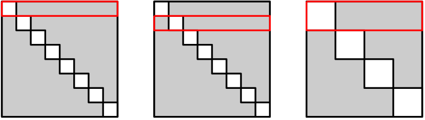
(a) (b) (c)
The basis matrices that span the row spaces of the offdiagonal blocks for any leaf are built through the same procedure, but starting with the sample matrix defined by (20.9). For instance, we form the sample matrix
| (20.11) |
and then compute the ID of to build a basis matrix and an index vector such that
The choice to use the interpolatory decomposition in factorizing the off-diagonal blocks is essential to making the linear complexity compression scheme work. In particular, observe that once we have formed the row and column IDs of all the leaf boxes, we automatically obtain rank- factorizations of all the corresponding sibling interaction matrices. For instance, if is a sibling pair consisting of two leaf nodes, then the sibling interaction matrix admits the factorization
| (20.12) |
In order to evaluate (20.12), we merely need to form the matrix .
Once the leaf nodes have all been processed, we proceed to the next coarser level. Consider for instance the node with children and . Our task is in principle to build the long basis matrix that spans the columns of , which is the shaded matrix inside the red rectangle in Figure 14(c). (We say “in principle” since it will not actually be explicitly formed.) To this end, we define the sample matrix
The idea is now to repeat the same technique that we used for the leaf boxes, and write
| (20.13) |
It turns out that we can evaluate (20.13) very efficiently: The block is made up of the two diagonal blocks and , and the two off-diagonal blocks and . Now observe that at this point in the execution of the algorithm, we have compressed representations of all these blocks available. Using this information, we form a short sample matrix of size that we can compress to build the basis matrix and the associated index vector in an ID of . ∎
20.8. Butterfly matrices
An interesting class of rank-structured matrices arises from a generalization of the discrete Fourier transform. These so called “butterfly matrices” provide a data sparse format for many matrices that appear in the analysis of neural networks, wave propagation problems, and signal processing (?, ?, ?). This format involves an additional complication in comparison to the HODLR and HBS formats in that it requires different tessellations of the matrix, as illustrated for a simple case in Figure 15. It can be demonstrated that when all of the resulting submatrices are of numerically low rank, the matrix as a whole can be written (approximately) as a product of sparse matrices, in a manner analogous to the butterfly representation of an FFT (?, Sec. 10.4).

Randomization has proven to be a powerful tool for finding butterfly representations of matrices. The techniques involved are more complex than the methods described in Sections 20.4 – 20.6 due to the multiplicative nature of the representation, and typically involve iterative refinement rather than direct approximation (?, ?, ?). Similar techniques played an essential role in a recent ground breaking paper (?) that exploits butterfly representations to directly solve linear systems arising from the modeling of scattering problems in the high frequency regime.
20.9. Applications of rank-structured matrices in data analysis
The machinery for working with rank-structured hierarchical matrices that we have described can be used also for the kernel matrices discussed in Section 19 that arise in machine learning and computational statistics. For instance, ? demonstrate that data sparse formats of this type can be very effective for simulating Gaussian processes in low dimensional spaces.
When the underlying dimension grows, the techniques that we have described so far become uncompetitive. Even would be considered a stretch. Fortunately, significant progress has recently been made towards extending the essential ideas to higher dimensions. For instance, ? describe a technique that is designed to uncover intrinsic lower dimensional structures that are often present in sets of points that ostensibly live in higher dimensional spaces. The idea is to use randomized algorithms both for organizing the points into a hierarchical tree (that induces the tessellation of the matrix) and for computing low rank approximations to the resulting admissible blocks. The authors report promising numerical results for a wide selection of kernel matrices.
In this context, it is as we saw in Section 19 rarely possible to execute a matrix-vector multiplication, or even to evaluate more than a tiny fraction of the entries of the matrix. This means on the one hand that sampling must form an integral part of the compression strategy, and on the other that firm performance guarantees are typically not available. The saving grace is that when a kernel matrix is used for learning and data analysis, a rough approximation is often sufficient.
Remark 20.6 (Geometry oblivious methods).
A curious observation is that techniques developed for kernel matrices appear to also be applicable for certain symmetric positive definite (pd) matrices that are not explicitly presented as kernel matrices. This is a consequence of the well known fact that any pd matrix admits a factorization
| (20.14) |
for a so called “Gramian matrix” . (If the eigenvalue decomposition of takes the form , then a matrix of the form is a Gramian if and only if is unitary.) The factorization (20.14) says that the entries of are formed by the inner products between the columns of ,
| (20.15) |
where is the ’th column of (the “Gram vector”) and where the is the inner product kernel of Example 19.7. At this point, it becomes plausible that the techniques of (?) for kernel matrices associated with points in high dimensional spaces may apply to certain pd matrices. The key to make this work is the observation that it is not necessary to explicitly form the Gram factors . All that is needed in order to organize the points are relative distances and angles between the points, and we can evaluate these from the matrix entries of , via the formula
The resulting technique was presented in (?) as a “geometry oblivious FMM (GOFMM)”, along with numerical evidence of its usefulness for important classes of matrices.
References
- [1]
- [2] [] D. Achlioptas (2003), Database-friendly random projections: Johnson-Lindenstrauss with binary coins, Vol. 66, pp. 671–687. Special issue on PODS 2001 (Santa Barbara, CA).
- [3]
- [4] [] D. Achlioptas and F. McSherry (2001), Fast computation of low rank matrix approximations, in Proceedings of the Thirty-Third Annual ACM Symposium on Theory of Computing, ACM, New York, pp. 611–618.
- [5]
- [6] [] D. Achlioptas and F. McSherry (2007), ‘Fast computation of low-rank matrix approximations’, J. ACM 54(2), Art. 9, 19.
- [7]
- [8] [] R. Ahlswede and A. Winter (2002), ‘Strong converse for identification via quantum channels’, IEEE Trans. Inform. Theory 48(3), 569–579.
- [9]
- [10] [] N. Ailon and B. Chazelle (2006), Approximate nearest neighbors and the fast johnson-lindenstrauss transform, in Proceedings of the thirty-eighth annual ACM symposium on Theory of computing, ACM, pp. 557–563.
- [11]
- [12] [] N. Ailon and B. Chazelle (2009), ‘The fast Johnson-Lindenstrauss transform and approximate nearest neighbors’, SIAM J. Comput. 39(1), 302–322.
- [13]
- [14] [] A. Alaoui and M. W. Mahoney (2015), Fast randomized kernel ridge regression with statistical guarantees, in Advances in Neural Information Processing Systems 28 (C. Cortes, N. D. Lawrence, D. D. Lee, M. Sugiyama and R. Garnett, eds), Curran Associates, Inc., pp. 775–783.
- [15]
- [16] [] N. Alon, P. B. Gibbons, Y. Matias and M. Szegedy (2002), Tracking join and self-join sizes in limited storage, Vol. 64, pp. 719–747. Special issue on PODS 1999 (Philadelphia, PA).
- [17]
- [18] [] N. Alon, Y. Matias and M. Szegedy (1999), The space complexity of approximating the frequency moments, Vol. 58, pp. 137–147. Twenty-eighth Annual ACM Symposium on the Theory of Computing (Philadelphia, PA, 1996).
- [19]
- [20] [] S. Ambikasaran, D. Foreman-Mackey, L. Greengard, D. W. Hogg and M. O’Neil (2015), ‘Fast direct methods for gaussian processes’, IEEE transactions on pattern analysis and machine intelligence 38(2), 252–265.
- [21]
- [22] [] D. Amelunxen, M. Lotz, M. B. McCoy and J. A. Tropp (2014), ‘Living on the edge: phase transitions in convex programs with random data’, Inf. Inference 3(3), 224–294.
- [23]
- [24] [] T. Ando (2005), The Schur complement and its applications, Vol. 4 of Numerical Methods and Algorithms, Springer-Verlag, New York, chapter Schur complements and matrix inequalities: Operator-theoretic approach, pp. 137–162.
- [25]
- [26] [] M. A. Arcones and E. Gine (1992), ‘On the bootstrap of and statistics’, Ann. Statist. 20(2), 655–674.
- [27]
- [28] [] B. Arras, M. Bachmayr and A. Cohen (2019), ‘Sequential sampling for optimal weighted least squares approximations in hierarchical spaces’, SIAM J. Math. Data Sci. 1(1), 189–207.
- [29]
- [30] [] H. Avron (2018), ‘Randomized Riemannian preconditioning for quadratically constrained problems’. Slides, Workshop on Randomized Numerical Linear Algebra, Simons Institute, UC-Berkeley.
- [31]
- [32] [] H. Avron, K. Clarkson and D. Woodruff (2017), ‘Faster kernel ridge regression using sketching and preconditioning’, SIAM Journal on Matrix Analysis and Applications 38(4), 1116–1138.
- [33]
- [34] [] H. Avron, A. Druinsky and A. Gupta (2015), ‘Revisiting asynchronous linear solvers: Provable convergence rate through randomization’, Journal of the ACM (JACM) 62(6), 51.
- [35]
- [36] [] H. Avron, M. Kapralov, C. Musco, C. Musco, A. Velingker and A. Zandieh (2019), A universal sampling method for reconstructing signals with simple fourier transforms, in Proceedings of the 51st Annual ACM SIGACT Symposium on Theory of Computing, STOC 2019, Association for Computing Machinery, New York, NY, USA, pp. 1051–1063.
- [37]
- [38] [] H. Avron, P. Maymounkov and S. Toledo (2010), ‘Blendenpik: Supercharging lapack’s least-squares solver’, SIAM Journal on Scientific Computing 32(3), 1217–1236.
- [39]
- [40] [] M. Baboulin, J. J. Dongarra, A. Rémy, S. Tomov and I. Yamazaki (2017), ‘Solving dense symmetric indefinite systems using gpus’, Concurrency and Computation: Practice and Experience.
- [41]
- [42] [] M. Baboulin, X. S. Li and F.-H. Rouet (2014), Using random butterfly transformations to avoid pivoting in sparse direct methods, in International Conference on High Performance Computing for Computational Science, Springer, pp. 135–144.
- [43]
- [44] [] F. Bach (2013), Sharp analysis of low-rank kernel matrix approximations, in Conference on Learning Theory, pp. 185–209.
- [45]
- [46] [] F. Bach (2017), ‘On the equivalence between kernel quadrature rules and random feature expansions’, Journal of Machine Learning Research 18(21), 1–38.
- [47]
- [48] [] F. R. Bach and M. Jordan (2005), Predictive low-rank decomposition for kernel methods, in ICML ’05: Proceedings of the 22Nd International Conference on Machine Learning, ACM, New York, NY, USA.
- [49]
- [50] [] Z. Bai and J. W. Silverstein (2010), Spectral analysis of large dimensional random matrices, Springer Series in Statistics, second edn, Springer, New York.
- [51]
- [52] [] Z. Bai, J. Demmel, J. Dongarra, A. Ruhe and H. van der Vorst (1987), Templates for the Solution of Algebraic Eigenvalue Problems: A Practical Guide (Software, Environments and Tools), 1st edn, SIAM, Philadelphia, PA.
- [53]
- [54] [] P. Baldi and R. Vershynin (2019), ‘Polynomial threshold functions, hyperplane arrangements, and random tensors’, SIAM J. Math. Data Sci. 1(4), 699–729.
- [55]
- [56] [] G. Ballard, J. Demmel, I. Dumitriu and A. Rusciano (2019), ‘A generalized randomized rank-revealing factorization’, arXiv preprint arXiv:1909.06524.
- [57]
- [58] [] J. Banks, J. G. Vargas, A. Kulkarni and N. Srivastava (2019), ‘Pseudospectral shattering, the sign function, and diagonalization in nearly matrix multiplication time’.
- [59]
- [60] [] J. Barnes and P. Hut (1986), ‘A hierarchical force-calculation algorithm’, Nature.
- [61]
- [62] [] J. Batson, D. A. Spielman and N. Srivastava (2014), ‘Twice-Ramanujan sparsifiers’, SIAM Rev. 56(2), 315–334.
- [63]
- [64] [] M. Bebendorf and R. Grzhibovskis (2006), ‘Accelerating galerkin bem for linear elasticity using adaptive cross approximation’, Mathematical Methods in the Applied Sciences 29(14), 1721–1747.
- [65]
- [66] [] R. Bhatia (1997), Matrix analysis, Vol. 169 of Graduate Texts in Mathematics, Springer-Verlag, New York.
- [67]
- [68] [] C. H. Bischof and G. Quintana-Ortí (1998), ‘Computing rank-revealing QR factorizations of dense matrices’, ACM Transactions on Mathematical Software 24(2), 226–253.
- [69]
- [70] [] S. Bôchner (1933), ‘Monotone Funktionen, Stieltjessche Integrale und harmonische Analyse’, Math. Ann. 108(1), 378–410.
- [71]
- [72] [] L. Bottou (2010), Large-scale machine learning with stochastic gradient descent, in Proceedings of COMPSTAT’2010 (Y. Lechevallier and G. Saporta, eds), Physica-Verlag HD, Heidelberg, pp. 177–186.
- [73]
- [74] [] S. Boucheron, G. Lugosi and P. Massart (2013), Concentration inequalities, Oxford University Press, Oxford. A nonasymptotic theory of independence, With a foreword by Michel Ledoux.
- [75]
- [76] [] J. Bourgain, S. Dirksen and J. Nelson (2015), ‘Toward a unified theory of sparse dimensionality reduction in Euclidean space’, Geom. Funct. Anal. 25(4), 1009–1088.
- [77]
- [78] [] C. Boutsidis, M. W. Mahoney and P. Drineas (2009), An improved approximation algorithm for the column subset selection problem, in Proceedings of the Twentieth Annual ACM-SIAM Symposium on Discrete Algorithms, SIAM, Philadelphia, PA, pp. 968–977.
- [79]
- [80] [] C. Boutsidis, D. P. Woodruff and P. Zhong (2016), Optimal principal component analysis in distributed and streaming models, in Proceedings of the forty-eighth annual ACM symposium on Theory of Computing, ACM, pp. 236–249.
- [81]
- [82] [] W. L. Briggs and V. E. Henson (1995), The DFT: An Owner’s Manual for the Discrete Fourier Transform, Society for Industrial and Applied Mathematics.
- [83]
- [84] [] K. Bringmann and K. Panagiotou (2017), ‘Efficient sampling methods for discrete distributions’, Algorithmica 79(2), 484–508.
- [85]
- [86] [] E. Candès, L. Demanet and L. Ying (2009), ‘A fast butterfly algorithm for the computation of fourier integral operators’, Multiscale Modeling & Simulation 7(4), 1727–1750.
- [87]
- [88] [] B. Carl (1985), ‘Inequalities of Bernstein-Jackson-type and the degree of compactness of operators in Banach spaces’, Ann. Inst. Fourier (Grenoble) 35(3), 79–118.
- [89]
- [90] [] Y. Carmon, J. C. Duchi, A. Sidford and K. Tian (2019), A rank-1 sketch for matrix multiplicative weights, in Proceedings of the Thirty-Second Conference on Learning Theory (A. Beygelzimer and D. Hsu, eds), Vol. 99 of Proceedings of Machine Learning Research, PMLR, Phoenix, USA, pp. 589–623.
- [91]
- [92] [] S. Chandrasekaran, M. Gu and W. Lyons (2005), ‘A fast adaptive solver for hierarchically semiseparable representations’, Calcolo 42(3-4), 171–185.
- [93]
- [94] [] V. Chandrasekaran, B. Recht, P. A. Parrilo and A. S. Willsky (2012), ‘The convex geometry of linear inverse problems’, Found. Comput. Math. 12(6), 805–849.
- [95]
- [96] [] M. Charikar, K. Chen and M. Farach-Colton (2004), Finding frequent items in data streams, Vol. 312, pp. 3–15. Automata, languages and programming.
- [97]
- [98] [] L. H. Y. Chen, L. Goldstein and Q.-M. Shao (2011), Normal approximation by Stein’s method, Probability and its Applications (New York), Springer, Heidelberg.
- [99]
- [100] [] X. Chen and E. Price (2019), Active regression via linear-sample sparsification, in Proceedings of the Thirty-Second Conference on Learning Theory (A. Beygelzimer and D. Hsu, eds), Vol. 99 of Proceedings of Machine Learning Research, PMLR, Phoenix, USA, pp. 663–695.
- [101]
- [102] [] Z. Chen and J. J. Dongarra (2005), ‘Condition numbers of Gaussian random matrices’, SIAM J. Matrix Anal. Appl. 27(3), 603–620.
- [103]
- [104] [] H. Cheng, Z. Gimbutas, P. Martinsson and V. Rokhlin (2005), ‘On the compression of low rank matrices’, SIAM Journal of Scientific Computing 26(4), 1389–1404.
- [105]
- [106] [] K. L. Clarkson and D. P. Woodruff (2009), Numerical linear algebra in the streaming model, in Proceedings of the 41st annual ACM symposium on Theory of computing, ACM, pp. 205–214.
- [107]
- [108] [] K. L. Clarkson and D. P. Woodruff (2013), Low rank approximation and regression in input sparsity time, in STOC’13—Proceedings of the 2013 ACM Symposium on Theory of Computing, ACM, New York, pp. 81–90.
- [109]
- [110] [] A. Cohen and G. Migliorati (2017), ‘Optimal weighted least-squares methods’, SMAI J. Comput. Math. 3, 181–203.
- [111]
- [112] [] A. Cohen, M. A. Davenport and D. Leviatan (2013), ‘On the stability and accuracy of least squares approximations’, Found. Comput. Math. 13(5), 819–834.
- [113]
- [114] [] E. Cohen and D. D. Lewis (1999), ‘Approximating matrix multiplication for pattern recognition tasks’, Journal of Algorithms 30(2), 211 – 252.
- [115]
- [116] [] M. B. Cohen (2016), Nearly tight oblivious subspace embeddings by trace inequalities, in Proceedings of the Twenty-Seventh Annual ACM-SIAM Symposium on Discrete Algorithms, ACM, New York, pp. 278–287.
- [117]
- [118] [] M. B. Cohen, R. Kyng, G. L. Miller, J. W. Pachocki, R. Peng, A. B. Rao and S. C. Xu (2014), Solving sdd linear systems in nearly mlog1/2n time, in Proceedings of the Forty-sixth Annual ACM Symposium on Theory of Computing, STOC ’14, ACM, New York, NY, USA, pp. 343–352.
- [119]
- [120] [] J. Cullum and W. E. Donath (1974), A block generalization of the -step Lanczos algorithm, Technical Report Report RC 4845 (21570), IBM Thomas J. Watson Research Center, Yorktown Heights, New York.
- [121]
- [122] [] T. Dao, A. Gu, M. Eichhorn, A. Rudra and C. Ré (2019), ‘Learning fast algorithms for linear transforms using butterfly factorizations’.
- [123]
- [124] [] K. R. Davidson and S. J. Szarek (2001), Local operator theory, random matrices and Banach spaces, in Handbook of the geometry of Banach spaces, Vol. I, North-Holland, Amsterdam, pp. 317–366.
- [125]
- [126] [] T. A. Davis, S. Rajamanickam and W. M. Sid-Lakhdar (2016), ‘A survey of direct methods for sparse linear systems’, Acta Numerica.
- [127]
- [128] [] J. Demmel, I. Dumitriu and O. Holtz (2007), ‘Fast linear algebra is stable’, Numerische Mathematik 108(1), 59–91.
- [129]
- [130] [] J. Demmel, L. Grigori, M. Hoemmen and J. Langou (2012), ‘Communication-optimal parallel and sequential QR and LU factorizations’, SIAM J. Sci. Comput. 34(1), A206–A239.
- [131]
- [132] [] J. W. Demmel, L. Grigori, M. Gu and H. Xiang (2015), ‘Communication avoiding rank revealing qr factorization with column pivoting’, SIAM Journal on Matrix Analysis and Applications 36(1), 55–89.
- [133]
- [134] [] J. D. Dixon (1983), ‘Estimating extremal eigenvalues and condition numbers of matrices’, SIAM J. Numer. Anal. 20(4), 812–814.
- [135]
- [136] [] E. Dobriban and S. Liu (2018), ‘Asymptotics for sketching in least squares regression’.
- [137]
- [138] [] P. Drineas and M. Mahoney (2018), Lectures on randomized linear algebra, in The Mathematics of Data (M. Mahoney, J. Duchi and A. Gilbert, eds), Vol. 25, American Mathematical Society, chapter 4, pp. 1 – 48. IAS/Park City Mathematics Series.
- [139]
- [140] [] P. Drineas and M. W. Mahoney (2005), ‘On the Nyström method for approximating a Gram matrix for improved kernel-based learning’, J. Mach. Learn. Res. 6, 2153–2175.
- [141]
- [142] [] P. Drineas, R. Kannan and M. W. Mahoney (2006a), ‘Fast Monte Carlo algorithms for matrices. I. Approximating matrix multiplication’, SIAM J. Comput. 36(1), 132–157.
- [143]
- [144] [] P. Drineas, R. Kannan and M. W. Mahoney (2006b), ‘Fast Monte Carlo algorithms for matrices. II. Computing a low-rank approximation to a matrix’, SIAM J. Comput. 36(1), 158–183.
- [145]
- [146] [] P. Drineas, R. Kannan and M. W. Mahoney (2006c), ‘Fast Monte Carlo algorithms for matrices. III. Computing a compressed approximate matrix decomposition’, SIAM J. Comput. 36(1), 184–206.
- [147]
- [148] [] P. Drineas, M. W. Mahoney and S. Muthukrishnan (2006d), Subspace sampling and relative-error matrix approximation: column-based methods, in Approximation, randomization and combinatorial optimization, Vol. 4110 of Lecture Notes in Comput. Sci., Springer, Berlin, pp. 316–326.
- [149]
- [150] [] P. Drineas, M. W. Mahoney and S. Muthukrishnan (2008), ‘Relative-error matrix decompositions’, SIAM J. Matrix Anal. Appl. 30(2), 844–881.
- [151]
- [152] [] J. A. Duersch and M. Gu (2017), ‘Randomized qr with column pivoting’, SIAM Journal on Scientific Computing 39(4), C263–C291.
- [153]
- [154] [] J. Duersch and M. Gu (2015), ‘True blas-3 performance qrcp using random sampling’. arXiv preprint #1509.06820.
- [155]
- [156] [] A. S. Edelman (1989), Eigenvalues and condition numbers of random matrices, ProQuest LLC, Ann Arbor, MI. Thesis (Ph.D.)–Massachusetts Institute of Technology.
- [157]
- [158] [] B. Efron (1982), The jackknife, the bootstrap and other resampling plans, Vol. 38 of CBMS-NSF Regional Conference Series in Applied Mathematics, Society for Industrial and Applied Mathematics (SIAM), Philadelphia, Pa.
- [159]
- [160] [] D. Feldman, M. Volkov and D. Rus (2016), Dimensionality reduction of massive sparse datasets using coresets, in Advances in Neural Information Processing Systems, pp. 2766–2774.
- [161]
- [162] [] Y. Feng, J. Xiao and M. Gu (2018), ‘Low-rank matrix approximations with flip-flop spectrum-revealing qr factorization’, arXiv preprint arXiv:1803.01982.
- [163]
- [164] [] R. D. Fierro, P. C. Hansen and P. S. K. Hansen (1999), ‘Utv tools: Matlab templates for rank-revealing utv decompositions’, Numerical Algorithms 20(2-3), 165–194.
- [165]
- [166] [] S. Fine and K. Scheinberg (2001), ‘Efficient SVM training using low-rank kernel representation’, Journal of Machine Learning Research 2, 243–264.
- [167]
- [168] [] J. K. Fitzsimons, M. A. Osborne, S. J. Roberts and J. F. Fitzsimons (2018), Improved stochastic trace estimators using mutually unbiased bases, in Uncertainty in Artificial Intelligence: Proceedings of the Thirty-Fourth Conference (A. Globerson and R. Silva, eds), AUAI Press, Monterey, CA.
- [169]
- [170] [] S. Foucart and H. Rauhut (2013), A mathematical introduction to compressive sensing, Applied and Numerical Harmonic Analysis, Birkhäuser/Springer, New York.
- [171]
- [172] [] A. Frieze, R. Kannan and S. Vempala (2004), ‘Fast Monte-Carlo algorithms for finding low-rank approximations’, J. ACM 51(6), 1025–1041.
- [173]
- [174] [] M. Ghashami, E. Liberty, J. M. Phillips and D. P. Woodruff (2016a), ‘Frequent directions: simple and deterministic matrix sketching’, SIAM J. Comput. 45(5), 1762–1792.
- [175]
- [176] [] M. Ghashami, D. J. Perry and J. Phillips (2016b), Streaming kernel principal component analysis, in Proceedings of the 19th International Conference on Artificial Intelligence and Statistics (A. Gretton and C. C. Robert, eds), Vol. 51 of Proceedings of Machine Learning Research, PMLR, Cadiz, Spain, pp. 1365–1374.
- [177]
- [178] [] P. Ghysels, X. S. Li, C. Gorman and F.-H. Rouet (2017), A robust parallel preconditioner for indefinite systems using hierarchical matrices and randomized sampling, in 2017 IEEE International Parallel and Distributed Processing Symposium (IPDPS), IEEE, pp. 897–906.
- [179]
- [180] [] A. Gionis, P. Indyk and R. Motwani (1999), Similarity search in high dimensions via hashing, in Proceedings of the 25th International Conference on Very Large Data Bases, VLDB ’99, Morgan Kaufmann Publishers Inc., San Francisco, CA, USA, pp. 518–529.
- [181]
- [182] [] D. A. Girard (1989), ‘A fast “Monte Carlo cross-validation” procedure for large least squares problems with noisy data’, Numer. Math. 56(1), 1–23.
- [183]
- [184] [] A. Gittens (2013), Topics in Randomized Numerical Linear Algebra, ProQuest LLC, Ann Arbor, MI. Thesis (Ph.D.)–California Institute of Technology.
- [185]
- [186] [] L. Goldstein, I. Nourdin and G. Peccati (2017), ‘Gaussian phase transitions and conic intrinsic volumes: Steining the Steiner formula’, Ann. Appl. Probab. 27(1), 1–47.
- [187]
- [188] [] G. H. Golub and G. Meurant (1994), Matrices, moments and quadrature, in Numerical analysis 1993 (Dundee, 1993), Vol. 303 of Pitman Res. Notes Math. Ser., Longman Sci. Tech., Harlow, pp. 105–156.
- [189]
- [190] [] G. H. Golub and G. Meurant (2010), Matrices, moments and quadrature with applications, Princeton Series in Applied Mathematics, Princeton University Press, Princeton, NJ.
- [191]
- [192] [] G. H. Golub and R. Underwood (1977), The block Lanczos method for computing eigenvalues, in Mathematical software, III (Proc. Sympos., Math. Res. Center, Univ. Wisconsin, Madison, Wis., 1977), Academic Press, New York, pp. 361–377. Publ. Math. Res. Center, No. 39.
- [193]
- [194] [] G. H. Golub and C. F. Van Loan (2013), Matrix computations, Johns Hopkins Studies in the Mathematical Sciences, fourth edn, Johns Hopkins University Press, Baltimore, MD.
- [195]
- [196] [] G. H. Golub, F. T. Luk and M. L. Overton (1981), ‘A block Lánczos method for computing the singular values of corresponding singular vectors of a matrix’, ACM Trans. Math. Software 7(2), 149–169.
- [197]
- [198] [] I. J. Good (1977), ‘A new formula for -statistics’, Ann. Statist. 5(1), 224–228.
- [199]
- [200] [] A. Gopal and P.-G. Martinsson (2018), ‘The PowerURV algorithm for computing rank-revealing full factorizations’.
- [201]
- [202] [] Y. Gordon (1988), On Milman’s inequality and random subspaces which escape through a mesh in , in Geometric aspects of functional analysis (1986/87), Vol. 1317 of Lecture Notes in Math., Springer, Berlin, pp. 84–106.
- [203]
- [204] [] S. A. Goreinov, I. V. Oseledets, D. V. Savostyanov, E. E. Tyrtyshnikov and N. L. Zamarashkin (2010), How to find a good submatrix, in Matrix Methods: Theory, Algorithms And Applications: Dedicated to the Memory of Gene Golub, World Scientific, pp. 247–256.
- [205]
- [206] [] S. Goreinov, N. Zamarashkin and E. Tyrtyshnikov (1997), ‘Pseudo-skeleton approximations by matrices of maximal volume’, Mathematical Notes.
- [207]
- [208] [] R. Gower and P. Richtarik (2015a), ‘Randomized iterative methods for linear systems’, SIAM Journal on Matrix Analysis and Applications 36(4), 1660–1690.
- [209]
- [210] [] R. Gower, F. Hanzely, P. Richtarik and S. U. Stich (2018), Accelerated stochastic matrix inversion: General theory and speeding up bfgs rules for faster second-order optimization, in Advances in Neural Information Processing Systems 31 (S. Bengio, H. Wallach, H. Larochelle, K. Grauman, N. Cesa-Bianchi and R. Garnett, eds), Curran Associates, Inc., pp. 1619–1629.
- [211]
- [212] [] R. M. Gower and P. Richtárik (2015b), ‘Randomized iterative methods for linear systems’, SIAM J. Matrix Anal. Appl. 36(4), 1660–1690.
- [213]
- [214] [] L. Grasedyck and W. Hackbusch (2003), ‘Construction and arithmetics of -matrices’, Computing 70(4), 295–334.
- [215]
- [216] [] S. Gratton and D. Titley-Peloquin (2018), ‘Improved bounds for small-sample estimation’, SIAM J. Matrix Anal. Appl. 39(2), 922–931.
- [217]
- [218] [] L. Greengard and V. Rokhlin (1987), ‘A fast algorithm for particle simulations’, J. Comput. Phys. 73(2), 325–348.
- [219]
- [220] [] G. R. Grimmett and D. R. Stirzaker (2001), Probability and random processes, third edn, Oxford University Press, New York.
- [221]
- [222] [] M. Gu (2015), ‘Subspace iteration randomization and singular value problems’, SIAM J. Sci. Comput. 37(3), A1139–A1173.
- [223]
- [224] [] M. Gu and S. C. Eisenstat (1996), ‘Efficient algorithms for computing a strong rank-revealing QR factorization’, SIAM J. Sci. Comput. 17(4), 848–869.
- [225]
- [226] [] H. Guo, Y. Liu, J. Hu and E. Michielssen (2017), ‘A butterfly-based direct integral-equation solver using hierarchical lu factorization for analyzing scattering from electrically large conducting objects’, IEEE Transactions on Antennas and Propagation 65(9), 4742–4750.
- [227]
- [228] [] W. Hackbusch (1999), ‘A sparse matrix arithmetic based on H-matrices; Part I: Introduction to H-matrices’, Computing 62, 89–108.
- [229]
- [230] [] W. Hackbusch, B. Khoromskij and S. Sauter (2002), On -matrices, in Lectures on Applied Mathematics, Springer Berlin, pp. 9–29.
- [231]
- [232] [] N. Halko, P. G. Martinsson and J. A. Tropp (2011a), ‘Finding structure with randomness: probabilistic algorithms for constructing approximate matrix decompositions’, SIAM Rev. 53(2), 217–288.
- [233]
- [234] [] N. Halko, P.-G. Martinsson, Y. Shkolnisky and M. Tygert (2011b), ‘An algorithm for the principal component analysis of large data sets’, SIAM J. Sci. Comput. 33(5), 2580–2594.
- [235]
- [236] [] R. Hamid, Y. Xiao, A. Gittens and D. Decoste (2014), Compact random feature maps, in Proceedings of the 31st International Conference on Machine Learning (E. P. Xing and T. Jebara, eds), Vol. 32 of Proceedings of Machine Learning Research, PMLR, Bejing, China, pp. 19–27.
- [237]
- [238] [] J. Hampton and A. Doostan (2015), ‘Coherence motivated sampling and convergence analysis of least squares polynomial chaos regression’, Computer Methods in Applied Mechanics and Engineering 290, 73 – 97.
- [239]
- [240] [] P. Hennig and M. A. Osborne (2019), ‘probabilistic-numerics.org’.
- [241]
- [242] [] M. R. Hestenes and E. Stiefel (1952), Methods of conjugate gradients for solving linear systems, Vol. 49, NBS Washington, DC.
- [243]
- [244] [] R. A. Horn and C. R. Johnson (2013), Matrix analysis, second edn, Cambridge University Press, Cambridge.
- [245]
- [246] [] M. F. Hutchinson (1990), ‘A stochastic estimator of the trace of the influence matrix for Laplacian smoothing splines’, Comm. Statist. Simulation Comput. 19(2), 433–450.
- [247]
- [248] [] P. Indyk and R. Motwani (1999), Approximate nearest neighbors: towards removing the curse of dimensionality, in STOC ’98 (Dallas, TX), ACM, New York, pp. 604–613.
- [249]
- [250] [] R. Jin, T. G. Kolda and R. Ward (2019), ‘Faster johnson-lindenstrauss transforms via kronecker products’.
- [251]
- [252] [] W. B. Johnson and J. Lindenstrauss (1984), Extensions of Lipschitz mappings into a Hilbert space, in Conference in modern analysis and probability (New Haven, Conn., 1982), Vol. 26 of Contemp. Math., Amer. Math. Soc., Providence, RI, pp. 189–206.
- [253]
- [254] [] I. M. Johnstone (2001), ‘On the distribution of the largest eigenvalue in principal components analysis’, Ann. Statist. 29(2), 295–327.
- [255]
- [256] [] W. D. Joubert and G. F. Carey (1991), Parellelizable restarted iterative methods for nonsymmetric linear systems, Center for Numerical Analysis Report CNA-251, UT-Austin.
- [257]
- [258] [] M. Kac (1956), Foundations of kinetic theory, in Proceedings of the Third Berkeley Symposium on Mathematical Statistics and Probability, 1954–1955, vol. III, University of California Press, Berkeley and Los Angeles, pp. 171–197.
- [259]
- [260] [] W. Kahan (1966), ‘Numerical linear algebra’, Canadian Math. Bull 9(6), 757–801.
- [261]
- [262] [] R. Kannan and S. Vempala (2017), ‘Randomized algorithms in numerical linear algebra’, Acta Numerica 26, 95–135.
- [263]
- [264] [] P. Kar and H. Karnick (2012), Random feature maps for dot product kernels, in Proceedings of the Fifteenth International Conference on Artificial Intelligence and Statistics (N. D. Lawrence and M. Girolami, eds), Vol. 22 of Proceedings of Machine Learning Research, PMLR, La Palma, Canary Islands, pp. 583–591.
- [265]
- [266] [] S. P. Kasiviswanathan, M. Rudelson, A. Smith and J. Ullman (2010), The price of privately releasing contingency tables and the spectra of random matrices with correlated rows, in STOC’10—Proceedings of the 2010 ACM International Symposium on Theory of Computing, ACM, New York, pp. 775–784.
- [267]
- [268] [] W. Kong and G. Valiant (2017), ‘Spectrum estimation from samples’, Ann. Statist. 45(5), 2218–2247.
- [269]
- [270] [] V. S. Koroljuk and Y. V. Borovskich (1994), Theory of -statistics, Vol. 273 of Mathematics and its Applications, Kluwer Academic Publishers Group, Dordrecht. Translated from the 1989 Russian original by P. V. Malyshev and D. V. Malyshev and revised by the authors.
- [271]
- [272] [] F. Krahmer and R. Ward (2011), ‘New and improved johnson-lindenstrauss embeddings via the restricted isometry property’, SIAM J. Math. Anal. 43(3), 1269–1281.
- [273]
- [274] [] D. Kressner, M. Steinlechner and B. Vandereycken (2016), ‘Preconditioned low-rank riemannian optimization for linear systems with tensor product structure’, SIAM Journal on Scientific Computing 38(4), A2018–A2044.
- [275]
- [276] [] J. Kuczyński and H. Woźniakowski (1992), ‘Estimating the largest eigenvalue by the power and Lanczos algorithms with a random start’, SIAM J. Matrix Anal. Appl. 13(4), 1094–1122.
- [277]
- [278] [] R. Kueng (2019), 2-designs minimize variance of trace estimators, Unpublished manuscript.
- [279]
- [280] [] S. Kumar, M. Mohri and A. Talwalkar (2012), ‘Sampling methods for the Nyström method’, J. Mach. Learn. Res. 13, 981–1006.
- [281]
- [282] [] S. Kurz, O. Rain and S. Rjasanow (2002), ‘The adaptive cross-approximation technique for the 3d boundary-element method’, IEEE transactions on Magnetics 38(2), 421–424.
- [283]
- [284] [] R. Kyng (2017), Approximate Gaussian elimination, ProQuest LLC, Ann Arbor, MI. Thesis (Ph.D.)–Yale University.
- [285]
- [286] [] R. Kyng and S. Sachdeva (2016), Approximate Gaussian elimination for Laplacians—fast, sparse, and simple, in 57th Annual IEEE Symposium on Foundations of Computer Science—FOCS 2016, IEEE Computer Soc., Los Alamitos, CA, pp. 573–582.
- [287]
- [288] [] R. Kyng, Y. T. Lee, R. Peng, S. Sachdeva and D. A. Spielman (2016), Sparsified Cholesky and multigrid solvers for connection Laplacians, in STOC’16—Proceedings of the 48th Annual ACM SIGACT Symposium on Theory of Computing, ACM, New York, pp. 842–850.
- [289]
- [290] [] Q. Le, T. Sarlós and A. Smola (2013), Fastfood - computing hilbert space expansions in loglinear time, in Proceedings of the 30th International Conference on Machine Learning (S. Dasgupta and D. McAllester, eds), Vol. 28 of Proceedings of Machine Learning Research, PMLR, Atlanta, Georgia, USA, pp. 244–252.
- [291]
- [292] [] M. Ledoux and M. Talagrand (1991), Probability in Banach spaces, Vol. 23 of Ergebnisse der Mathematik und ihrer Grenzgebiete (3) [Results in Mathematics and Related Areas (3)], Springer-Verlag, Berlin. Isoperimetry and processes.
- [293]
- [294] [] D. Leventhal and A. S. Lewis (2010), ‘Randomized methods for linear constraints: convergence rates and conditioning’, Math. Oper. Res. 35(3), 641–654.
- [295]
- [296] [] Z. Leyk and H. Woźniakowski (1998), ‘Estimating a largest eigenvector by Lanczos and polynomial algorithms with a random start’, Numer. Linear Algebra Appl. 5(3), 147–164.
- [297]
- [298] [] H. Li, G. C. Linderman, A. Szlam, K. P. Stanton, Y. Kluger and M. Tygert (2017), ‘Algorithm 971: an implementation of a randomized algorithm for principal component analysis’, ACM Trans. Math. Software 43(3), Art. 28, 14.
- [299]
- [300] [] M. Li, W. Bi, J. T. Kwok and B. Lu (2015a), ‘Large-scale nyström kernel matrix approximation using randomized svd’, IEEE Transactions on Neural Networks and Learning Systems 26(1), 152–164.
- [301]
- [302] [] Y. Li and H. Yang (2017), ‘Interpolative butterfly factorization’, SIAM Journal on Scientific Computing 39(2), A503–A531.
- [303]
- [304] [] Y. Li, H. L. Nguyen and D. P. Woodruff (2014a), On sketching matrix norms and the top singular vector, in Proceedings of the Twenty-Fifth Annual ACM-SIAM Symposium on Discrete Algorithms, ACM, New York, pp. 1562–1581.
- [305]
- [306] [] Y. Li, H. L. Nguyen and D. P. Woodruff (2014b), Turnstile streaming algorithms might as well be linear sketches, in STOC’14—Proceedings of the 2014 ACM Symposium on Theory of Computing, ACM, New York, pp. 174–183.
- [307]
- [308] [] Y. Li, H. Yang and L. Ying (2018), ‘Multidimensional butterfly factorization’, Applied and Computational Harmonic Analysis 44(3), 737 – 758.
- [309]
- [310] [] Y. Li, H. Yang, E. R. Martin, K. L. Ho and L. Ying (2015b), ‘Butterfly factorization’, Multiscale Modeling & Simulation 13(2), 714–732.
- [311]
- [312] [] E. Liberty (2009), Accelerated Dense Random Projections, PhD thesis, Computer Science, Yale University.
- [313]
- [314] [] E. Liberty, F. Woolfe, P.-G. Martinsson, V. Rokhlin and M. Tygert (2007), ‘Randomized algorithms for the low-rank approximation of matrices’, Proc. Natl. Acad. Sci. USA 104(51), 20167–20172.
- [315]
- [316] [] L.-H. Lim and J. Weare (2017), ‘Fast randomized iteration: Diffusion monte carlo through the lens of numerical linear algebra’, SIAM Review 59(3), 547–587.
- [317]
- [318] [] L. Lin, J. Lu and L. Ying (2011), ‘Fast construction of hierarchical matrix representation from matrix–vector multiplication’, Journal of Computational Physics 230(10), 4071 – 4087.
- [319]
- [320] [] N. Linial, E. London and Y. Rabinovich (1995), ‘The geometry of graphs and some of its algorithmic applications’, Combinatorica 15(2), 215–245.
- [321]
- [322] [] M. E. Lopes (2019), ‘Estimating the algorithmic variance of randomized ensembles via the bootstrap’, Ann. Statist. 47(2), 1088–1112.
- [323]
- [324] [] D. Lopez-Paz, S. Sra, A. Smola, Z. Ghahramani and B. Schölkopf (2014), Randomized nonlinear component analysis, in Proceedings of the 31st International Conference on Machine Learning (E. P. Xing and T. Jebara, eds), Vol. 32 of Proceedings of Machine Learning Research, PMLR, Bejing, China, pp. 1359–1367.
- [325]
- [326] [] F. Lust-Piquard (1986), ‘Inégalités de Khintchine dans ’, C. R. Acad. Sci. Paris Sér. I Math. 303(7), 289–292.
- [327]
- [328] [] L. Mackey, M. I. Jordan, R. Y. Chen, B. Farrell and J. A. Tropp (2014), ‘Matrix concentration inequalities via the method of exchangeable pairs’, Ann. Probab. 42(3), 906–945.
- [329]
- [330] [] M. W. Mahoney (2011), ‘Randomized algorithms for matrices and data’, Foundations and Trends® in Machine Learning 3(2), 123–224.
- [331]
- [332] [] M. W. Mahoney and P. Drineas (2009), ‘Cur matrix decompositions for improved data analysis’, Proceedings of the National Academy of Sciences 106(3), 697–702.
- [333]
- [334] [] O. A. Malik and S. Becker (2019), ‘Guarantees for the kronecker fast johnson-lindenstrauss transform using a coherence and sampling argument’.
- [335]
- [336] [] W. B. March, B. Xiao and G. Biros (2015), ‘Askit: Approximate skeletonization kernel-independent treecode in high dimensions’, SIAM Journal on Scientific Computing 37(2), A1089–A1110.
- [337]
- [338] [] M. B. Marcus and G. Pisier (1981), Random Fourier series with applications to harmonic analysis, Vol. 101 of Annals of Mathematics Studies, Princeton University Press, Princeton, N.J.; University of Tokyo Press, Tokyo.
- [339]
- [340] [] P. Martinsson (2011), ‘A fast randomized algorithm for computing a hierarchically semiseparable representation of a matrix’, SIAM Journal on Matrix Analysis and Applications 32(4), 1251–1274.
- [341]
- [342] [] P. Martinsson (2015), ‘Blocked rank-revealing qr factorizations: How randomized sampling can be used to avoid single-vector pivoting’. arXiv preprint #1505.08115.
- [343]
- [344] [] P. Martinsson and V. Rokhlin (2005), ‘A fast direct solver for boundary integral equations in two dimensions’, J. Comp. Phys. 205(1), 1–23.
- [345]
- [346] [] P. Martinsson and S. Voronin (2016), ‘A randomized blocked algorithm for efficiently computing rank-revealing factorizations of matrices’, SIAM Journal on Scientific Computing 38(5), S485–S507.
- [347]
- [348] [] P.-G. Martinsson (2016), ‘Compressing rank-structured matrices via randomized sampling’, SIAM Journal on Scientific Computing 38(4), A1959–A1986.
- [349]
- [350] [] P.-G. Martinsson (2018), Randomized methods for matrix computations, in The Mathematics of Data (M. Mahoney, J. Duchi and A. Gilbert, eds), Vol. 25, American Mathematical Society, chapter 4, pp. 187 – 231. IAS/Park City Mathematics Series.
- [351]
- [352] [] P.-G. Martinsson (2019), Fast Direct Solvers for Elliptic PDEs, Vol. CB96 of CBMS-NSF conference series, SIAM.
- [353]
- [354] [] P.-G. Martinsson, V. Rokhlin and M. Tygert (2006a), A randomized algorithm for the approximation of matrices, Technical Report Yale CS research report YALEU/DCS/RR-1361, Yale University, Computer Science Department.
- [355]
- [356] [] P. Martinsson, G. Quintana Orti and N. Heavner (2019), ‘randUTV: A blocked randomized algorithm for computing a rank-revealing UTV factorization’, arXiv preprint arXiv:1703.00998. Accepted for publication by ACM TOMS.
- [357]
- [358] [] P. Martinsson, G. Quintana-Ortí, N. Heavner and R. van de Geijn (2017), ‘Householder qr factorization with randomization for column pivoting (hqrrp)’, SIAM Journal on Scientific Computing 39(2), C96–C115.
- [359]
- [360] [] P. Martinsson, V. Rokhlin and M. Tygert (2006b), ‘On interpolation and integration in finite-dimensional spaces of bounded functions’, Comm. Appl. Math. Comput. Sci pp. 133–142.
- [361]
- [362] [] R. Mathias and G. Stewart (1993), ‘A block {QR} algorithm and the singular value decomposition’, Linear Algebra and its Applications 182, 91 – 100.
- [363]
- [364] [] M. B. McCoy and J. A. Tropp (2013), The achievable performance of convex demixing, ACM Technical Report 2017-02, Caltech, Pasadena, CA.
- [365]
- [366] [] M. B. McCoy and J. A. Tropp (2014), ‘From Steiner formulas for cones to concentration of intrinsic volumes’, Discrete Comput. Geom. 51(4), 926–963.
- [367]
- [368] [] C. Melgaard and M. Gu (2015), ‘Gaussian elimination with randomized complete pivoting’, arXiv preprint arXiv:1511.08528.
- [369]
- [370] [] S. Mendelson, H. Rauhut and R. Ward (2018), ‘Improved bounds for sparse recovery from subsampled random convolutions’, Ann. Appl. Probab. 28(6), 3491–3527.
- [371]
- [372] [] X. Meng and M. W. Mahoney (2013), Low-distortion subspace embeddings in input-sparsity time and applications to robust linear regression, in STOC’13—Proceedings of the 2013 ACM Symposium on Theory of Computing, ACM, New York, pp. 91–100.
- [373]
- [374] [] X. Meng, M. A. Saunders and M. W. Mahoney (2014), ‘LSRN: a parallel iterative solver for strongly over- or underdetermined systems’, SIAM J. Sci. Comput. 36(2), C95–C118.
- [375]
- [376] [] F. Mezzadri (2007), ‘How to generate random matrices from the classical compact groups’, Notices Amer. Math. Soc. 54(5), 592–604.
- [377]
- [378] [] E. Moulines and F. R. Bach (2011), Non-asymptotic analysis of stochastic approximation algorithms for machine learning, in Advances in Neural Information Processing Systems, pp. 451–459.
- [379]
- [380] [] R. J. Muirhead (1982), Aspects of multivariate statistical theory, John Wiley & Sons, Inc., New York. Wiley Series in Probability and Mathematical Statistics.
- [381]
- [382] [] C. Musco and C. Musco (2015), Randomized block Krylov methods for stronger and faster approximate singular value decomposition, in Advances in Neural Information Processing Systems 28 (C. Cortes, N. D. Lawrence, D. D. Lee, M. Sugiyama and R. Garnett, eds), Curran Associates, Inc., pp. 1396–1404.
- [383]
- [384] [] C. Musco and C. Musco (2017), Recursive sampling for the nystrom method, in Advances in Neural Information Processing Systems 30 (I. Guyon, U. V. Luxburg, S. Bengio, H. Wallach, R. Fergus, S. Vishwanathan and R. Garnett, eds), Curran Associates, Inc., pp. 3833–3845.
- [385]
- [386] [] C. Musco, C. Musco and A. Sidford (2018), Stability of the Lanczos method for matrix function approximation, in Proceedings of the Twenty-Ninth Annual ACM-SIAM Symposium on Discrete Algorithms, SIAM, Philadelphia, PA, pp. 1605–1624.
- [387]
- [388] [] S. Muthukrishnan (2005), ‘Data streams: Algorithms and applications’, Foundations and Trends® in Theoretical Computer Science 1(2), 117–236.
- [389]
- [390] [] T. N. A. G. (NAG) (2019), ‘The nag library mark 27’. https://www.nag.com/content/naglibrary-mark27.
- [391]
- [392] [] R. M. Neal (1996), Priors for Infinite Networks, Springer New York, New York, NY, pp. 29–53.
- [393]
- [394] [] D. Needell and J. A. Tropp (2014), ‘Paved with good intentions: analysis of a randomized block kaczmarz method’, Linear Algebra and its Applications 441, 199–221.
- [395]
- [396] [] D. Needell, R. Ward and N. Srebro (2014), Stochastic gradient descent, weighted sampling, and the randomized kaczmarz algorithm, in Advances in neural information processing systems, pp. 1017–1025.
- [397]
- [398] [] J. Nelson and H. L. Nguyen (2013), OSNAP: faster numerical linear algebra algorithms via sparser subspace embeddings, in 2013 IEEE 54th Annual Symposium on Foundations of Computer Science—FOCS 2013, IEEE Computer Soc., Los Alamitos, CA, pp. 117–126.
- [399]
- [400] [] E. J. Nyström (1930), ‘Über Die Praktische Auflösung von Integralgleichungen mit Anwendungen auf Randwertaufgaben’, Acta Math. 54(1), 185–204.
- [401]
- [402] [] E. Oja (1982), ‘A simplified neuron model as a principal component analyzer’, J. Math. Biol. 15(3), 267–273.
- [403]
- [404] [] R. I. Oliveira (2009a), ‘Concentration of the adjacency matrix and of the laplacian in random graphs with independent edges’.
- [405]
- [406] [] R. I. Oliveira (2009b), ‘On the convergence to equilibrium of Kac’s random walk on matrices’, Ann. Appl. Probab. 19(3), 1200–1231.
- [407]
- [408] [] M. O’Neil (2007), A new class of analysis-based fast transforms, PhD thesis, Mathematics, Yale University.
- [409]
- [410] [] S. Oymak and J. A. Tropp (2018), ‘Universality laws for randomized dimension reduction, with applications’, Inf. Inference 7(3), 337–446.
- [411]
- [412] [] R. Pagh (2013), ‘Compressed matrix multiplication’, ACM Trans. Comput. Theory.
- [413]
- [414] [] V. Y. Pan and L. Zhao (2017), ‘Numerically safe gaussian elimination with no pivoting’, Linear Algebra and its Applications 527, 349 – 383.
- [415]
- [416] [] C. H. Papadimitriou, P. Raghavan, H. Tamaki and S. Vempala (2000), Latent semantic indexing: a probabilistic analysis, Vol. 61, pp. 217–235. Special issue on the Seventeenth ACM SIGACT-SIGMOD-SIGART Symposium on Principles of Database Systems (Seattle, WA, 1998).
- [417]
- [418] [] H. Park and L. Eldén (1995), ‘Downdating the rank-revealing urv decomposition’, SIAM Journal on Matrix Analysis and Applications 16(1), 138–155.
- [419]
- [420] [] D. Parker (1995), Random butterfly transformations with applications in computational linear algebra, Technical Report CSD-950023, UCLA.
- [421]
- [422] [] B. N. Parlett (1998), The symmetric eigenvalue problem, Vol. 20 of Classics in Applied Mathematics, Society for Industrial and Applied Mathematics (SIAM), Philadelphia, PA. Corrected reprint of the 1980 original.
- [423]
- [424] [] N. Pham and R. Pagh (2013), Fast and scalable polynomial kernels via explicit feature maps, in Proceedings of the 19th ACM SIGKDD International Conference on Knowledge Discovery and Data Mining, KDD ’13, ACM, New York, NY, USA, pp. 239–247.
- [425]
- [426] [] M. Pilanci and M. J. Wainwright (2015), ‘Randomized sketches of convex programs with sharp guarantees’, IEEE Trans. Inform. Theory 61(9), 5096–5115.
- [427]
- [428] [] M. Pilanci and M. J. Wainwright (2016), ‘Iterative Hessian sketch: fast and accurate solution approximation for constrained least-squares’, J. Mach. Learn. Res. 17, Paper No. 53, 38.
- [429]
- [430] [] N. S. Pillai and A. Smith (2017), ‘Kac’s walk on -sphere mixes in steps’, Ann. Appl. Probab. 27(1), 631–650.
- [431]
- [432] [] U. Porod (1996), ‘The cut-off phenomenon for random reflections’, Ann. Probab. 24(1), 74–96.
- [433]
- [434] [] F. Pourkamali-Anaraki and S. Becker (2019), ‘Improved fixed-rank nyström approximation via qr decomposition: Practical and theoretical aspects’, Neurocomputing 363, 261 – 272.
- [435]
- [436] [] A. Rahimi and B. Recht (2008), Random features for large-scale kernel machines, in Advances in Neural Information Processing Systems 20 (J. C. Platt, D. Koller, Y. Singer and S. T. Roweis, eds), Curran Associates, Inc., pp. 1177–1184.
- [437]
- [438] [] A. Rahimi and B. Recht (2009), Weighted sums of random kitchen sinks: Replacing minimization with randomization in learning, in Advances in Neural Information Processing Systems 21 (D. Koller, D. Schuurmans, Y. Bengio and L. Bottou, eds), Curran Associates, Inc., pp. 1313–1320.
- [439]
- [440] [] H. Rauhut and R. Ward (2012), ‘Sparse Legendre expansions via -minimization’, J. Approx. Theory 164(5), 517–533.
- [441]
- [442] [] H. Rauhut and R. Ward (2016), ‘Interpolation via weighted minimization’, Appl. Comput. Harmon. Anal. 40(2), 321–351.
- [443]
- [444] [] H. Rauhut, J. Romberg and J. A. Tropp (2012), ‘Restricted isometries for partial random circulant matrices’, Appl. Comput. Harmon. Anal. 32(2), 242–254.
- [445]
- [446] [] P. Richtárik and M. Takáč (2017), ‘Stochastic reformulations of linear systems: Algorithms and convergence theory’.
- [447]
- [448] [] V. Rokhlin and M. Tygert (2008), ‘A fast randomized algorithm for overdetermined linear least-squares regression’, Proc. Natl. Acad. Sci. USA 105(36), 13212–13217.
- [449]
- [450] [] V. Rokhlin, A. Szlam and M. Tygert (2009), ‘A randomized algorithm for principal component analysis’, SIAM Journal on Matrix Analysis and Applications 31(3), 1100–1124.
- [451]
- [452] [] J. S. Rosenthal (1994), ‘Random rotations: characters and random walks on ’, Ann. Probab. 22(1), 398–423.
- [453]
- [454] [] N. Ross (2011), ‘Fundamentals of Stein’s method’, Probab. Surv. 8, 210–293.
- [455]
- [456] [] M. Rudelson (1999), ‘Random vectors in the isotropic position’, J. Funct. Anal. 164(1), 60–72.
- [457]
- [458] [] M. Rudelson (2012), ‘Row products of random matrices’, Adv. Math. 231(6), 3199–3231.
- [459]
- [460] [] M. Rudelson and R. Vershynin (2007), ‘Sampling from large matrices: an approach through geometric functional analysis’, J. ACM 54(4), Art. 21, 19.
- [461]
- [462] [] M. Rudelson and R. Vershynin (2008), ‘On sparse reconstruction from Fourier and Gaussian measurements’, Comm. Pure Appl. Math. 61(8), 1025–1045.
- [463]
- [464] [] A. Rudi and L. Rosasco (2017), Generalization properties of learning with random features, in Advances in Neural Information Processing Systems 30 (I. Guyon, U. V. Luxburg, S. Bengio, H. Wallach, R. Fergus, S. Vishwanathan and R. Garnett, eds), Curran Associates, Inc., pp. 3215–3225.
- [465]
- [466] [] A. Rudi, D. Calandriello, L. Carratino and L. Rosasco (2018), On fast leverage score sampling and optimal learning, in Advances in Neural Information Processing Systems 31 (S. Bengio, H. Wallach, H. Larochelle, K. Grauman, N. Cesa-Bianchi and R. Garnett, eds), Curran Associates, Inc., pp. 5672–5682.
- [467]
- [468] [] A. Rudi, R. Camoriano and L. Rosasco (2015), Less is more: Nyström computational regularization, in Advances in Neural Information Processing Systems 28 (C. Cortes, N. D. Lawrence, D. D. Lee, M. Sugiyama and R. Garnett, eds), Curran Associates, Inc., pp. 1657–1665.
- [469]
- [470] [] A. Rudi, L. Carratino and L. Rosasco (2017), Falkon: An optimal large scale kernel method, in Advances in Neural Information Processing Systems 30 (I. Guyon, U. V. Luxburg, S. Bengio, H. Wallach, R. Fergus, S. Vishwanathan and R. Garnett, eds), Curran Associates, Inc., pp. 3888–3898.
- [471]
- [472] [] Y.-L. K. Samo and S. Roberts (2015), ‘Generalized spectral kernels’.
- [473]
- [474] [] A. Sankar, D. A. Spielman and S.-H. Teng (2006), ‘Smoothed analysis of the condition numbers and growth factors of matrices’, SIAM J. Matrix Anal. Appl. 28(2), 446–476.
- [475]
- [476] [] T. Sarlós (2006), Improved approximation algorithms for large matrices via random projections, in 2006 47th Annual IEEE Symposium on Foundations of Computer Science (FOCS’06), pp. 143–152.
- [477]
- [478] [] I. J. Schoenberg (1942), ‘Positive definite functions on spheres’, Duke Math. J. 9, 96–108.
- [479]
- [480] [] B. Schölkopf and A. Smola (2001), Learning with Kernels, MIT Press, Cambridge, MA.
- [481]
- [482] [] B. Schölkopf, A. Smola and K.-R. Müller (1996), Nonlinear component analysis as a kernel eigenvalue problem, Technical report 44, Max-Planck-Institut für biologische Kybernetik.
- [483]
- [484] [] M. Simchowitz, A. E. Alaoui and B. Recht (2017), ‘On the gap between strict-saddles and true convexity: An omega(log d) lower bound for eigenvector approximation’.
- [485]
- [486] [] N. J. A. Sloane (1983), Encrypting by random rotations, in Cryptography (Burg Feuerstein, 1982), Vol. 149 of Lecture Notes in Comput. Sci., Springer, Berlin, pp. 71–128.
- [487]
- [488] [] D. C. Sorensen and M. Embree (2016), ‘A deim induced cur factorization’, SIAM Journal on Scientific Computing 38(3), A1454–A1482.
- [489]
- [490] [] D. A. Spielman and N. Srivastava (2011), ‘Graph sparsification by effective resistances’, SIAM J. Comput. 40(6), 1913–1926.
- [491]
- [492] [] B. Sriperumbudur and Z. Szabo (2015), Optimal rates for random fourier features, in Advances in Neural Information Processing Systems 28 (C. Cortes, N. D. Lawrence, D. D. Lee, M. Sugiyama and R. Garnett, eds), Curran Associates, Inc., pp. 1144–1152.
- [493]
- [494] [] G. Stewart (1994), ‘UTV decompositions’, PITMAN RESEARCH NOTES IN MATHEMATICS SERIES pp. 225–225.
- [495]
- [496] [] G. Stewart (1998), Matrix Algorithms Volume 1: Basic Decompositions, SIAM.
- [497]
- [498] [] G. Stewart (1999), ‘The QLP approximation to the singular value decomposition’, SIAM Journal on Scientific Computing 20(4), 1336–1348.
- [499]
- [500] [] G. W. Stewart (2001), Matrix algorithms volume 2: eigensystems, Vol. 2, Siam.
- [501]
- [502] [] M. Stojnic (2010), optimization and its various thresholds in compressed sensing, in 2010 IEEE International Conference on Acoustics, Speech and Signal Processing, pp. 3910–3913.
- [503]
- [504] [] G. Strang (2019), Linear algebra and learning from data, Wellesley-Cambridge Press.
- [505]
- [506] [] V. Strassen (1969), ‘Gaussian elimination is not optimal’, Numerische mathematik 13(4), 354–356.
- [507]
- [508] [] T. Strohmer and R. Vershynin (2009), ‘A randomized Kaczmarz algorithm with exponential convergence’, J. Fourier Anal. Appl. 15(2), 262–278.
- [509]
- [510] [] Y. Sun, Y. Guo, J. A. Tropp and M. Udell (2018), Tensor random projection for low memory dimension reduction, in NeurIPS Workshop on Relational Representation Learning.
- [511]
- [512] [] Z. Szabo and B. Sriperumbudur (2019), On kernel derivative approximation with random fourier features, in Proceedings of Machine Learning Research (K. Chaudhuri and M. Sugiyama, eds), Vol. 89 of Proceedings of Machine Learning Research, PMLR, pp. 827–836.
- [513]
- [514] [] S.-H. Teng (2010), The Laplacian paradigm: emerging algorithms for massive graphs, in Theory and applications of models of computation, Vol. 6108 of Lecture Notes in Comput. Sci., Springer, Berlin, pp. 2–14.
- [515]
- [516] [] C. Thrampoulidis and B. Hassibi (2015), ‘Isotropically random orthogonal matrices: Performance of lasso and minimum conic singular values’.
- [517]
- [518] [] C. Thrampoulidis, S. Oymak and B. Hassibi (2014), ‘The gaussian min-max theorem in the presence of convexity’.
- [519]
- [520] [] C. Thurau, K. Kersting and C. Bauckhage (2012), Deterministic cur for improved large-scale data analysis: An empirical study, in Proceedings of the 2012 SIAM International Conference on Data Mining, SIAM, pp. 684–695.
- [521]
- [522] [] N. Tomczak-Jaegermann (1974), ‘The moduli of smoothness and convexity and the Rademacher averages of trace classes ’, Studia Math. 50, 163–182.
- [523]
- [524] [] J.-F. Ton, S. Flaxman, D. Sejdinovic and S. Bhatt (2018), ‘Spatial mapping with gaussian processes and nonstationary fourier features’, Spatial Statistics 28, 59 – 78. One world, one health.
- [525]
- [526] [] L. N. Trefethen and D. Bau III (1997), Numerical linear algebra, Vol. 50, Siam.
- [527]
- [528] [] T. Trogdon (2017), ‘On spectral and numerical properties of random butterfly matrices’, Appl. Math. Lett. 95, 48–58.
- [529]
- [530] [] J. A. Tropp (2011a), ‘Freedman’s inequality for matrix martingales’, Electron. Commun. Probab. 16, 262–270.
- [531]
- [532] [] J. A. Tropp (2011b), ‘Improved analysis of the subsampled randomized Hadamard transform’, Adv. Adapt. Data Anal. 3(1-2), 115–126.
- [533]
- [534] [] J. A. Tropp (2012a), ‘A comparison principle for functions of a uniformly random subspace’, Probab. Theory Related Fields 153(3-4), 759–769.
- [535]
- [536] [] J. A. Tropp (2012b), ‘User-friendly tail bounds for sums of random matrices’, Found. Comput. Math. 12(4), 389–434.
- [537]
- [538] [] J. A. Tropp (2015), ‘An introduction to matrix concentration inequalities’, Foundations and Trends in Machine Learning 8(1-2), 1–230.
- [539]
- [540] [] J. A. Tropp (2016), The expected norm of a sum of independent random matrices: an elementary approach, in High dimensional probability VII, Vol. 71 of Progr. Probab., Springer, [Cham], pp. 173–202.
- [541]
- [542] [] J. A. Tropp (2018), Analysis of randomized block krylov methods, Under revision.
- [543]
- [544] [] J. A. Tropp (2019), Matrix concentration and computational linear algebra, CMS Lecture Notes 2019-01, Caltech, Pasadena, CA.
- [545]
- [546] [] J. A. Tropp, M. B. Wakin, M. F. Duarte, D. Baron and R. G. Baraniuk (2006), Random filters for compressive sampling and reconstruction, in 2006 IEEE International Conference on Acoustics Speech and Signal Processing Proceedings, Vol. 3, pp. III–III.
- [547]
- [548] [] J. A. Tropp, A. Yurtsever, M. Udell and V. Cevher (2017a), Fixed-rank approximation of a positive-semidefinite matrix from streaming data, in Advances in Neural Information Processing Systems 30 (I. Guyon, U. V. Luxburg, S. Bengio, H. Wallach, R. Fergus, S. Vishwanathan and R. Garnett, eds), Curran Associates, Inc., pp. 1225–1234.
- [549]
- [550] [] J. A. Tropp, A. Yurtsever, M. Udell and V. Cevher (2017b), ‘Practical sketching algorithms for low-rank matrix approximation’, SIAM Journal on Matrix Analysis and Applications 38(4), 1454–1485.
- [551]
- [552] [] J. A. Tropp, A. Yurtsever, M. Udell and V. Cevher (2017c), ‘Practical sketching algorithms for low-rank matrix approximation’, SIAM J. Matrix Anal. Appl. 38(4), 1454–1485.
- [553]
- [554] [] J. A. Tropp, A. Yurtsever, M. Udell and V. Cevher (2019), ‘Streaming low-rank matrix approximation with an application to scientific simulation’, SIAM J. Sci. Comput. 41(4), A2430–A2463.
- [555]
- [556] [] S. Ubaru, J. Chen and Y. Saad (2017), ‘Fast estimation of via stochastic Lanczos quadrature’, SIAM J. Matrix Anal. Appl. 38(4), 1075–1099.
- [557]
- [558] [] E. Ullah, P. Mianjy, T. V. Marinov and R. Arora (2018), Streaming kernel pca with random features, in Advances in Neural Information Processing Systems 31 (S. Bengio, H. Wallach, H. Larochelle, K. Grauman, N. Cesa-Bianchi and R. Garnett, eds), Curran Associates, Inc., pp. 7311–7321.
- [559]
- [560] [] J. Upadhyay (2016), ‘Fast and space-optimal low-rank factorization in the streaming model with application in differential privacy’, arXiv preprint arXiv:1604.01429.
- [561]
- [562] [] Y. Urano (2013), A fast randomized algorithm for linear least-squares regression via sparse transforms, Masters thesis, New York University.
- [563]
- [564] [] R. Van Handel (2016), Probability in high dimension, Apc 550 lecture notes, Princeton Univ.
- [565]
- [566] [] R. Vershynin (2018), High-dimensional probability, Vol. 47 of Cambridge Series in Statistical and Probabilistic Mathematics, Cambridge University Press, Cambridge. An introduction with applications in data science, With a foreword by Sara van de Geer.
- [567]
- [568] [] R. Vershynin (2019), ‘Concentration inequalities for random tensors’.
- [569]
- [570] [] S. Voronin and P.-G. Martinsson (2017), ‘Efficient algorithms for cur and interpolative matrix decompositions’, Advances in Computational Mathematics 43(3), 495–516.
- [571]
- [572] [] S. F. D. Waldron (2018), An introduction to finite tight frames, Applied and Numerical Harmonic Analysis, Birkhäuser/Springer, New York.
- [573]
- [574] [] S. Wang (2019), ‘Simple and almost assumption-free out-of-sample bound for random feature mapping’.
- [575]
- [576] [] S. Wang, A. Gittens and M. W. Mahoney (2019), ‘Scalable kernel k-means clustering with nyström approximation: Relative-error bounds’, J. Mach. Learn. Res. 20(1), 431–479.
- [577]
- [578] [] R. C. Whaley and J. J. Dongarra (1998), Automatically tuned linear algebra software, in Proceedings of the 1998 ACM/IEEE Conference on Supercomputing, SC ’98, IEEE Computer Society, Washington, DC, USA, pp. 1–27.
- [579]
- [580] [] C. K. I. Williams and M. Seeger (2001), Using the nyström method to speed up kernel machines, in Advances in Neural Information Processing Systems 13 (T. K. Leen, T. G. Dietterich and V. Tresp, eds), MIT Press, pp. 682–688.
- [581]
- [582] [] D. P. Woodruff (2014), ‘Sketching as a tool for numerical linear algebra’, Foundations and Trends in Theoretical Computer Science 10(1-2), 1 – 157.
- [583]
- [584] [] F. Woolfe, E. Liberty, V. Rokhlin and M. Tygert (2008), ‘A fast randomized algorithm for the approximation of matrices’, Appl. Comput. Harmon. Anal. 25(3), 335–366.
- [585]
- [586] [] W. K. Wootters and B. D. Fields (1989), ‘Optimal state-determination by mutually unbiased measurements’, Annals of Physics 191(2), 363 – 381.
- [587]
- [588] [] J. Xia (2013), ‘Randomized sparse direct solvers’, SIAM Journal on Matrix Analysis and Applications 34(1), 197–227.
- [589]
- [590] [] J. Xia, S. Chandrasekaran, M. Gu and X. S. Li (2010), ‘Fast algorithms for hierarchically semiseparable matrices’, Numerical Linear Algebra with Applications 17(6), 953–976.
- [591]
- [592] [] J. Xiao, M. Gu and J. Langou (2017), Fast parallel randomized qr with column pivoting algorithms for reliable low-rank matrix approximations, in 2017 IEEE 24th International Conference on High Performance Computing (HiPC), IEEE, pp. 233–242.
- [593]
- [594] [] C. D. Yu, J. Levitt, S. Reiz and G. Biros (2017a), Geometry-oblivious fmm for compressing dense spd matrices, in Proceedings of the International Conference for High Performance Computing, Networking, Storage and Analysis, ACM, p. 53.
- [595]
- [596] [] W. Yu, Y. Gu, J. Li, S. Liu and Y. Li (2017b), ‘Single-pass pca of large high-dimensional data’.
- [597]
- [598] [] Q. Yuan, M. Gu and B. Li (2018), Superlinear convergence of randomized block lanczos algorithm, in 2018 IEEE International Conference on Data Mining (ICDM), pp. 1404–1409.
- [599]
- [600] [] F. Zhang, ed. (2005), The Schur complement and its applications, Vol. 4 of Numerical Methods and Algorithms, Springer-Verlag, New York.
- [601]
- [602] [] A. Zouzias (2013), Randomized primitives for linear algebra and applications, Phd thesis, University of Toronto, Toronto.
- [603]