Gold Nanoparticles Passivated with Functionalized Alkylthiols: Simulations of Solvation in the Infinite Dilution Limit

Abstract

Solvation of gold nanoparticles passivated with end group functionalized alkylthiols, namely CH₃, NH₂ or COOH is studied in solvents of varying degrees of repulsion-dispersion and electrostatic interactions ranging from strongly polar SPC/E water to modified hybrid water models, where the Lennard-Jones contribution to the potential energy is enhanced relative to SPC/E to completely non-polar, decane. The effects due to solvent reorganization around the nanoparticle as a function of the ligand and solvent chemistry are monitored using the nanoparticle-solvent pair correlation functions and tetrahedral order parameter. The solvent penetration inside the ligand shell is maximum for decane, indicating better solute-solvent interaction in decane compared to other solvents. The COOH end group functionalized nanoparticle breaks the tetrahedral structure of water molecules more as compared to other nanoparticles used in this study. The ligand reorganization and its effect on solvation are monitored using radial density profiles (RDPs), radius of gyration ($R_{g}$) and ligand asymmetry parameter ($\langle\Delta\rangle$). RDP and $R_{g}$ values show significant stretching of ligands in decane than in model waters, which is also consistent with $\langle\Delta\rangle$. The ligand shell anisotropy for all nanoparticles is maximum in SPC/E water and minimum in decane. The isotropic potential of mean force ($V_{PMF}(r)$) between two identical end group functionalized nanoparticles have been calculated in vacuum, SPC/E water and H3.00 modified hybrid water, which consistently shows attractive well depth. Distance-dependent fluctuation driven anisotropy has also been examined. The implications for self-assembly of passivated gold nanoparticles from aqueous dispersions as well as the dependence of calculated quantities on ligand and solvent chemistry are highlighted.

I Introduction

Inorganic nano-cores passivated with different ligands with charged or uncharged tails self-organize into unique complex structures and show various physical, chemical and biological phenomena, which also depend on size and shape of the passivated nanoparticleNie, Petukhova, and Kumacheva (2010); Daniel and Astruc (2004); Bishop et al. (2009); Walker et al. (2011); Ung, Liz-Marzan, and Mulaveny (2001); Tang et al. (1994); Balazs, Emrick, and Russell (2006); Fu et al. (2008); Wu et al. (2002); Eastman et al. (2001); Wang, Xu, and Choi (1999). The advantage of these size-dependent properties can be further magnified and tailored by obtaining self-assembly of these nanoparticles into supraparticular assemblies of varying dimensions and superlatticesDaniel and Astruc (2004); Bishop et al. (2009); Tang, Kotov, and Giersig (2002); Kiely et al. (1998); Murray, Kagan, and Bawendi (2000, 1995); Shevchenko et al. (2006); Talapin et al. (2009); Li, Schnablegger, and Mann (1999); Tang et al. (2006); Zhang et al. (2006). In order to obtain an ordered 2D or 3D super-structure from self-assembly process, it is very important to get a stable dispersion of that particular nanoparticle (NP) in a suitable solvent. The passivation of the nano-core with suitable ligands leads to the formation of stable nanoparticle dispersions in various solvent media and is the initial step in order to obtain bulk nano-structures due to NPs self-organizing ability. The interaction between NPs and the subsequent formation of self-organized nano-structures not only depends on the shape, size and type of the nano-core but also on the ligands used for passivation and the solvent mediumMin et al. (2008); Bishop et al. (2009), since the solvation free energy also takes into account the ligand-ligand and ligand-solvent interactions. Hence, understanding the behaviour of different ligand passivated nanoparticles in various solvents and the reorganization of the solvent around the passivated nanoparticle is of prime importance in order to elucidate the reasons for the formation of unique structures due to self-assembly process and their relation to several phenomena.

In order to get a passivated nanoparticle, various combinations of nano-core and coatings have been reported in the literatureNie, Petukhova, and Kumacheva (2010); Daniel and Astruc (2004); Park et al. (2007); Bishop et al. (2009); Walker et al. (2011). The nano-core can be metal or its oxide, solid polymers, semiconductors; whereas coatings can be of a thin layer of a hard material on another material to obtain nanoshell particles or can be soft ligands such as small organic molecules, polymers or biological materials. The $Au$ core and the alkanethiol ligands have been extensively studied and the potential energy functions are well established to model such systemsDaniel and Astruc (2004); Lane and Grest (2010); Luedtke and Landman (1998); DeLong et al. (2010). The significance of this system in nanofiltration, drug delivery, biochemical sensors and optoelectronics and other fields have been well illustrated in the literatureHe et al. (2011a, b); Elghanian et al. (1997); Boisselier and Astruc (2009); Ghosh et al. (2008). In the present study, we have studied nanoparticles composed of $Au$ nano-core uniformly passivated with various end group functionalized alkylthiols.

The basic interactions governing the self-assembly process include van der Waals, magnetic, molecular surface forces, entropic effects and electrostatic interactionsBishop et al. (2009). Open structures can be obtained from self-assembly process due to electrostatic interactions, whereas, all other interactions or effects mostly form closed packed structuresBishop et al. (2009). The nanoscale self-assembly due to electrostatic interactions can be motivated by appropriate surface functionalization or $\omega$-functionalization of ligands used to passivate bare nano-cores. Experimentally, self-assembly of binary nanoparticles of almost equal size, passivated with oppositely charged $\omega$-functionalized alkylthiols are shown to form large 3D-crystals with diamond-like latticeKalsin et al. (2006); Bishop, Chevalier, and Grzybowski (2013). Each NP is surrounded by four oppositely charged neighbors at the vertices of the tetrahedron. Initial molecular dynamics studies of self-assembly of alkanethiol passivated gold nanoparticles have been done by Luedtke and LandmanLuedtke and Landman (1996, 1998). Subsequently, several studies have been performed to understand various aspects of alkanethiol coated gold nanoparticlesTay and Bresme (2005, 2006); Rapino and Zerbetto (2007); Ghorai and Glotzer (2007); Singh et al. (2007); Schapotschnikow, Pool, and Vlugt (2008); Djebaili et al. (2013); Lane and Grest (2014) followed by recent computational studies of $\omega$- or end group functionalized nanoparticles. Yang and Weng studied the structure and dynamics of water, when nanoparticles passivated with different neutral end group ligands are solvated in waterYang, Weng, and Chen (2011). Lane and Grest have also studied similar systems, focusing mainly on the spontaneous asymmetry of the passivated nanoparticles, which seem to depend on the chain length, particle size and thermodynamic variables like temperature and have significant implications on self-assembly processLane and Grest (2010). They have also further extended their study to understand the effects of charged ligands on coating asymmetryBolintineanu, Lane, and Grest (2014). Henz et al. have concentrated on determining the binding energy, density and solubility parameters of functionalized gold nanoparticles in vacuumHenz et al. (2011). Heikkila et al. have studied charged mono-layer $Au$ NPs with particular emphasis on electrostatic propertiesHeikkila et al. (2012). Giri and Spohr have also studied nanoparticles passivated with neutral and charged end group ligands with varying grafting densities of the ligands, with special attention on the penetration of water and ions in the soft coronaGiri and Spohr (2015). Lehn et al. have studied mixed-mono-layer protected gold nanoparticles, where only one of the ligands is end functionalizedLehn and Alexander-katz (2013).

In this study, we have carried out simulations of three types of $\omega$- or end group functionalized nanoparticles. The structure, thermodynamics and dynamics of a particular solvent also play an important role in the self-assembly process. Since the solvent properties can be easily varied either by changing the density or temperature, they provide an easy way to control the self-assembly process. Solvents are chosen to have varying degrees of repulsion-dispersion, electrostatic interactions and simple liquid character. The solvents considered in this study are SPC/E water model, modified hybrid water models (H1.56 and H3.00) and decane. SPC/E water is anomalous and polar in nature and has both repulsion-dispersion and electrostatic interactionsBerendsen, Grigera, and Straatsma (1987). For modified hybrid water models (H1.56 and H3.00), the degree of repulsion-dispersion contributions to the potential energy is increased by a factor of 1.56 and 3.00 with respect to SPC/ELynden-Bell and Debenedetti (2005), whereas decane is non-polarMishima and Stanley (1998). H1.56 and H3.00 are chosen, since they have been extensively studied by their developers as well as in our groupLynden-Bell and Debenedetti (2005); Lynden-Bell and Head-Gordon (2006); Alejandre and Lynden-Bell (2007); Chatterjee et al. (2008); Lynden-Bell (2010); Prasad and Chakravarty (2014). The modified hybrid water models were designed with a view to understand the relative contribution of LJ dispersion-repulsion term to the electrostatic term in determining the bulk and solvent properties of water. As the weight of the LJ term relative to the electrostatic term increases, a set of liquids which may be regarded as hybrids between SPC/E water and LJ liquid are created. Therefore, the modified hybrid water models may also be taken as representative of a range of strong and moderately polar liquidsPrasad and Chakravarty (2014). This particular study has been carried out to examine the effect of solvent interactions, structure and dynamics of the solvent and also the effect of end group functionalization on the thermodynamics of solvation, coating asymmetry and its implications on the self-assembly process.

The remaining paper has been organized as follows. Section II describes the various observables calculated in this study. Section III discusses the potential energy surface and the molecular dynamics simulation details. The results and conclusions are given in Sections IV and V, respectively.

II Solvation Structure and Thermodynamics

This section discusses the ideas which we have used to quantify the solvation structure and relate it to the thermodynamics of solvation of a single passivated nanoparticle in water, modified hybrid water models (H1.56 and H3.00) and decane. We have used Ben-Naim approach in order to understand the solvation behaviourBen-Naim (1978); Nayar et al. (2012). In all our single nanoparticle simulations at constant volume and temperature, the rigid gold-core is held fixed, keeping the center of mass of the gold-core fixed at the center of the solvent box, which eliminates the translational and rotational motions of the gold nano-core. The ligand and solvent molecules are free to reorganize themselves under the influence of each other. The pair correlation function, $g_{ns}(r)$, between the center of mass of the gold nano-core and the oxygen atoms of water (water as solvent) and decane monomer units (decane as solvent) describes the reorganization of solvent molecules around the ligand passivated nanoparticle. The pair correlation function, $g_{ns}(r)$, acts as central structural property, which can be used to define other important solvation properties like solvent excess ($n^{E}_{s}$), the local ($\Delta S^{loc}_{ns}$) and long-range ($\Delta S^{long}_{ns}$) contribution to entropy to quantify the solvation behaviour of individual nanoparticles.

The solvent excess, $n^{E}_{s}$, is defined in terms of the Kirkwood-Buff integral asKirkwood and Buff (1951); Lal, Plummer, and Smith (2006)

$$n^{E}_{s}={4\pi\rho_{i}}\int^{\infty}_{0}(g_{ns}(r)-1)r^{2}dr$$ (1)

where $\rho_{i}$ is the number density of oxygen atoms or decane monomer units depending on the solvent used. $n^{E}_{s}$ acts as a quantitative measure of the affinity of the solute for the given solvent by estimating the excess number of solvent molecules around an infinitely dilute solute moleculePetsche and Debenedetti (1989); Debenedetti and Mohamed (1989).

Since the rigid gold core is held fixed, the entropy will mostly be associated with the reorganization of the ligand and solvent molecules under the influence of each other.

II.1 Entropy of the Ligand Shell

The upper bound to the entropy of the flexible, long-chain ligand corona called the ligand shell configurational entropy, $S_{L}$, can be estimated by the Schlitter’s method using the covariances of the ligand atomic coordinates using the formulaSchlitter (1993),

$$S_{abs}<S_{L}=\frac{1}{2}k_{B}\ln\left|{\bf{1}}+\frac{k_{B}Te^{2}}{\hbar^{2}}\bf{M}^{1/2}\sigma\bf{M}^{1/2}\right|$$ (2)

where, $k_{B}$ is the Boltzmann constant, $e$ is the Euler number and is equal to $\exp(1)$, $\bf{M}$ is the 3N-dimensional diagonal matrix having masses of $N$ atoms of corresponding chains, $T$ is the simulation temperature and $\sigma$ is the covariance of the ligand atomic coordinates, defined as

$$\left<\sigma_{ij}\right>=\left<(x_{i}-\left<x_{i}\right>)(x_{j}-\left<x_{j}\right>)\right>$$ (3)

where, $x_{i}$ and $x_{j}$ are the Cartesian coordinates of $i^{th}$ and $j^{th}$ atoms. Since, the ligand shell configurational entropy, $S_{L}$, is the upper bound to entropy, it will always be greater than the absolute entropy of the system, $S_{abs}$. The entropy is calculated by using coordinates of ligand atoms after fitting each configuration with respect to the first frame of the trajectory in order to eliminate the translational and rotational motions of the ligand.

II.2 Entropy due to Solvent Reorganization

The change in entropy due to solvent reorganization around the passivated nanoparticle is estimated using nanoparticle-solvent pair correlation function. The total entropy associated with the reorganization of the solvent molecules around the ligand passivated nanoparticle is given as the sum of entropies arising due to the local ordering of solvent molecules and a long-range correction term to the entropy of solvation asLazaridis (1998a, b)

$$\Delta S^{tot}_{ns}=\Delta S^{loc}_{ns}+\Delta S^{long}_{ns}$$ (4)

The local entropic contribution due to solvent ordering around a spherically symmetric solute, $\Delta S^{loc}_{ns}$, can be written in terms of $g_{ns}(r)$ as

$$\Delta S_{ns}^{loc}/k=-4\pi\rho_{i}\int^{\infty}_{0}(g_{ns}(r)\ln g_{ns}(r))r^{2}dr$$ (5)

and the long-range correction term is defined in terms of Kirkwood-Buff integral as

$$\Delta S_{ns}^{long}/k=4\pi\rho_{i}\int^{\infty}_{0}(g_{ns}(r)-1)r^{2}dr$$ (6)

The fluctuations of the soft ligand corona around the passivated nanoparticle give rise to a form of anisotropy, which is an inherent property of single nanoparticles with small size and high surface curvatureLane and Grest (2010); Salerno et al. (2014); Bozorgui et al. (2013). This inherent anisotropy is quantified by calculating the mass dipole vector, $\vec{\Delta}$, between the center of mass of the gold nano-core and the ligand corona as shown in Figure 1 and also the probability distribution of the mass dipole vector, $P(\vec{\Delta})$Bozorgui et al. (2013); Jabes et al. (2014); Yadav et al. (2016). We have used $\vec{\Delta}$ and $P(\vec{\Delta})$ to estimate the degree of inherent anisotropy.

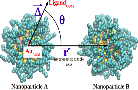
Figure 1: Schematic diagram illustrating the mass dipole vector, $\vec{\Delta}$, and the orientation of the mass dipole vector with respect to the inter-nanoparticle separation vector ($\vec{r}$). The snapshot is for two Au₁₄₀(SC₁₀)₆₂ nanoparticles in vacuum at 300 K for the pair separation of 55 $\mathring{A}$ . The sulfur atoms are shown in yellow and carbon in cyan. $Au_{COM}$ and $Ligand_{COM}$ represent the center of mass of the gold nano-core and ligand shell, respectively. The mass dipole vector, $\vec{\Delta}$, is defined as the vector connecting the $Au_{COM}$ and $Ligand_{COM}$. $\theta$ is the angle between the $\vec{\Delta}$ and the inter-nanoparticle axis ($\vec{r}$), joining the center of masses of the two nanoparticles.

II.3 Potentials of Mean Force

Using the simulations of a pair of identical nanoparticles in different solvent media, we have computed the isotropic potential of mean force and an unusual form of anisotropy called emergent anisotropy, which depends on the pair separation between the two nanoparticles.

Consider two nanoparticles A and B with position vectors ${\bf{r}_{A}}$ and ${\bf{r}_{B}}$ as shown in Figure 1. The free energy change as a function of the pair separation, $r=|\bf{r}_{A}-\bf{r}_{B}|$, gives the conventional isotropic potential of mean force (PMF), $V_{PMF}(r)$. We have used constrained molecular dynamics techniqueJabes et al. (2014); Trzesniak, Kunz, and Gunsteren (2007); Li et al. (2007); Schapotschnikow, Pool, and Vlugt (2008); Patel and Egorov (2007); Tay and Bresme (2005) to calculate the ensemble-averaged mean force at a pair separation $r$ between two nanoparticles A and B, which can be written as the derivative of the potential energy function, $U(r_{A},r_{B},r^{N})$ with respect to the pair separation $r=|\bf{r}_{A}-\bf{r}_{B}|$ asJabes et al. (2014)

$$\left\langle\frac{\partial U}{\partial r}\right\rangle=\frac{1}{2}\left[{\bf F}_{A}-{\bf F}_{B}\right]\cdot\hat{\bf r}\quad{\rm if}\quad m_{A}=m_{B}$$ (7)

where ${\bf F}_{A}$ and ${\bf F}_{b}$ are the forces acting on nanoparticles A and B due to all solvent molecules and $\hat{\bf r}$ is the unit vector in the direction $r=|\bf{r}_{A}-\bf{r}_{B}|$. Then the isotropic potential of mean force (PMF) can be obtained by integrating over a set of pair separations as

$$V_{PMF}(r)=\int_{\infty}^{r}\left\langle\frac{\partial U}{\partial r}\right\rangle dr-2k_{B}Tln\left(r\right)$$ (8)

where the last term is important when hard constraints are employed in MD simulationsTrzesniak, Kunz, and Gunsteren (2007); Li et al. (2007).

In case of two nanoparticles, the mass dipole vector ($\vec{\Delta}$) can be influenced by the presence of another approaching nanoparticle. The angle ($\theta$) between the mass dipole vector and the pair separation vector ($\bf{r}$) also provides relevant information about the orientation of the ligand shell or mass dipole as shown in Figure 1. Hence, the changes in the magnitude and orientation of the mass dipole vector in presence of an approaching second nanoparticle give rise to emergent anisotropy. Due to the presence of very high emergent anisotropy, the isotropic PMF becomes insufficient and does not provide reasonable explanations for many aspects of self-assembly process and hence, a two-dimensional anisotropic PMF, $V_{anis}(r,\cos\theta)$ is requiredBozorgui et al. (2013). In this paper, we compute the isotropic PMF between two identical end group functionalized ligand passivated nanoparticles in various solvent media and characterize the emergent anisotropy by calculating the change in magnitude and orientation of the mass dipole vector as a function of the pair separation between the two identical nanoparticles.

III Computational Details

This section gives the details of the potential energy surface and molecular dynamics simulation protocols used for $\omega$-functionalized ligand passivated gold nanoparticles in water, modified hybrid waters and decane. Earlier studies in order to validate the simulation protocols have already been done in our group for $Au_{140}$ passivated with alkanethiols in organic solventsYadav et al. (2016); Yadav and Chakravarty (2017). Subsections III.1 and III.2 describe the potential energy surface and molecular dynamics simulation details used in our studies.

III.1 Potential Energy Surface

III.1.1 Modified Hybrid Water Models

The modified hybrid water models were designed with a view to understanding the relative contribution of the Lennard-Jones dispersion-repulsion term to the electrostatic term in determining the bulk and solvent properties of waterLynden-Bell and Debenedetti (2005); Lynden-Bell and Head-Gordon (2006); Alejandre and Lynden-Bell (2007); Chatterjee et al. (2008); Lynden-Bell (2010). The potential energy form for the modified hybrid water models is written as

$$U=\lambda U_{LJ}+U_{ES}$$ (9)

where $U_{LJ}$ is the Lennard-Jones contribution and $U_{ES}$ is the electrostatic contribution. For the SPC/E model, the hybrid potential parameter, $\lambda$, is set to unity. The molecular geometry and partial charge distribution are constant for all values of $\lambda$. Increasing $\lambda$ increases the weight of the Lennard-Jones term relative to the electrostatic term, creating a set of fluids which may be regarded as hybrids between SPC/E water and a Lennard-Jones liquid. Therefore, the modified hybrid water models may also be taken as the representative of a range of strong and moderately polar liquids. The Lennard-Jones site is located on the oxygen atom of each water molecule and is characterized by the energy, $\epsilon_{OO}$, and size, $\sigma_{OO}$, parameters. The Lennard-Jones contribution to the potential energy for a pair of water molecules is given by

$$U_{LJ}\left(r\right)=4\epsilon_{OO}\left[\left(\frac{\sigma_{OO}}{r}\right)^{12}-\left(\frac{\sigma_{OO}}{r}\right)^{6}\right]$$ (10)

The electrostatic interaction between two water molecules $a$ and $b$ is given by

$$U_{ES}\left(r\right)=\sum_{i}\sum_{j}\frac{q_{i}q_{j}}{4\pi\epsilon_{0}r}$$ (11)

where $i$ and $j$ index the partial charges located on molecules $a$ and $b$. The parameters for the modified hybrid water models are summarized in Table SI of the supplementary materialsup .

III.1.2 Decane, Gold-core and Ligands

A rigid $Au_{140}$ truncated gold cluster was used in all our simulationskoishi and Tamaki (2005). Gold nano-cores of 140 $Au$ atoms were passivated with $\omega$-functionalized alkylthiols (SRX), where S, R and X represent thiol group (SH), common alkane chain (R = C₉H₁₈) and terminal group (X= CH₃, NH₂ and COOH), respectively. The TraPPE-UA model potentialMishima and Stanley (1998) was used for the thiol (SH), common alkane chain (R = C₉H₁₈), the terminal CH₃ and decane solvent, whereas all the atoms in NH₂ and COOH are simulated explicitly. Since, united atom model has been used for alkane chain (R = C₉H₁₈) and the terminal CH₃, so only symbol $C$ will be used further to denote a methyl or methylene unit. Hence, the different type of ligands used in this study can be written as SC₁₀, SC₉NH₂ and SC₉COOH. All non-bonded interactions were modeled via the Lennard-Jones and Coulomb potential. The parameters for similar atom pairsMishima and Stanley (1998); Tay and Bresme (2005); Landman and Luedtke (2004); Rizzo and Jorgensen (1999); Wick et al. (2005); Kamath, Cao, and Potoff (2004); Clifford, Bolton, and Ramjugernath (2006) are given in the Table SII of the supplementary materialsup . Lorentz-Berthelot combination rules were applied for dissimilar atom pairsLeach (1996). Bonds and bond angles were represented using harmonic stretching potential and harmonic bending potential, respectively. For 1-4 torsional interactions, we have used triple cosine and multi-harmonic potential. The parameters for harmonic stretching, harmonic bending, triple cosine and multi-harmonic potentialMishima and Stanley (1998); Tay and Bresme (2005); Landman and Luedtke (2004); Rizzo and Jorgensen (1999); Wick et al. (2005); Kamath, Cao, and Potoff (2004); Clifford, Bolton, and Ramjugernath (2006) are given in Tables SIII, SIV, SV and SVI, respectively of the supplementary materialsup . We would like to mention that we have used harmonic stretching for bonds instead of rigid bonds as used in original TraPPE-UA potential, both of which give similar resultsYadav et al. (2016). Additionally, the torsional equations related to terminal groups like NH₂ and COOH used in the literature are not present in LAMMPS MD package, hence, we have fitted these equations to obtain the constants for multi-harmonic potential. The fitted plots to obtain the constants for multi-harmonic potential are shown in Figures S1 and S2 of the supplementary materialsup . Non-bonded Morse potential was used for the gold-thiolate interaction; $U(r)=D_{e}((1-exp(-k(r-r_{e})))^{2}-1)$, where, $r_{e}$ = 2.9 $\mathring{A}$  is the equilibrium distance, $D_{e}$ = 38.6 kJ mol^-1 is the well depth, and $k$ = 1.3 $\mathring{A}$ ^-1 controls the range of the potentialLuedtke and Landman (1998).

III.2 Molecular Dynamics Simulation Details

We report molecular dynamics simulations of: (a) bulk water and decane, (b) single $\omega$-functionalized ligand passivated nanoparticle in vacuum, water and decane and (c) a pair of identical $\omega$-functionalized ligand passivated nanoparticles in vacuum and water. All simulations were performed using LAMMPS package with GPU accelerationPlimpton (1995). A timestep of 1 fs was used to integrate the equations of motion using the velocity-Verlet algorithm. The simulation temperature and pressure were maintained, wherever applicable, using Nose-Hoover thermostat and barostat with a relaxation time of 0.1 ps and 1 ps, respectively. Rigid body constraints in water were maintained using the SHAKE algorithm with tolerance value of 10^-6 $\mathring{A}$ . PPPM was used to account for the long-range electrostatic interactions. All non-bonded interactions were truncated at 14 $\mathring{A}$  during the solvation studies of passivated nanoparticles and in vacuum, a spherical cutoff of 30 $\mathring{A}$  was used.

III.2.1 Passivation of $Au_{140}$ Core in Vacuum

We followed the protocol similar to Luedtke and Landman for passivation of the gold core with all types of $\omega$-functionalized ligandsLuedtke and Landman (1996, 1998). The $Au_{140}$ core was placed at the center of a 100 $\mathring{A}$  $\times$ 100 $\mathring{A}$  $\times$ 100 $\mathring{A}$  cubic cell surrounded randomly with 100 decanethiol chains using PACKMOL packageMartínez et al. (2009). The system was equilibrated in NVT ensemble for 1 ns at 200 K in vacuum keeping the gold nano-core stationary. To ensure equilibration, rescaling of velocities were performed at every 10 steps. The system obtained after initial equilibration was heated from 200 to 500 K using a ramp of 2.5 K/ps. The system was then gradually cooled back from 500 to 300 K using a ramp of 0.5 K/ps. After the end of passivation protocol, 62 ligands were found attached to the gold core, consistent with the number of binding sites available. The number of attached ligands are also consistent with previous publicationsLuedtke and Landman (1996); Tay and Bresme (2005). All other excess ligand chains were removed. To ensure the stability of the passivated gold nanoparticle, 2 ns simulation at 300 K was performed. For passivation of the gold core using SC₉NH₂ and SC₉COOH ligand chains, the same procedure was followed, except that the system obtained after initial equilibration of 1 ns at 200 K was heated from 200 to 500 K using a ramp of 0.15 K/ps. Production runs of 20 ns were performed for all three types of passivated (Au₁₄₀(SC₁₀)₆₂, Au₁₄₀(SC₉NH₂)₆₂, Au₁₄₀(SC₉COOH)₆₂) nanoparticles in vacuum.

III.2.2 Solvation of a Passivated Nanoparticle

We have used water (SPC/E or H1.00), modified hybrid water (H1.56 and H3.00) and decane as a solvent. Solvent box for water was prepared by randomly packing the water molecules in 100 $\mathring{A}$  $\times$ 100 $\mathring{A}$  $\times$ 100 $\mathring{A}$  cubic simulation cell with density 1.00 g/cc (33428 water molecules). For decane, 0.73 g/cc density was used and decane molecules were also randomly packed in a cubic box of same dimensions (3090 decane molecules). The passivated nanoparticle was inserted in the solvent box by growing a void of 18 $\mathring{A}$  in radius in the center of the cubic box by using a soft repulsive spherical indent as shown in Figure S3 of the supplementary materialsup . After insertion, energy minimization of the system was done using conjugate gradient method in NVT ensemble for 1 ns. For all the solvated passivated nanoparticle systems prepared, equilibration runs of 10 ns were carried out in the NPT ensemble at 275 K and 300 K with 1 atm pressure. Once an equilibrium volume was obtained, the barostat was switched off and NVT production runs for 20 ns were performed at the same temperatures.

III.2.3 Potentials of Mean Force in Vacuum and Water

In vacuum, the two passivated nanoparticles were placed along the x-axis at a separation of 55 $\mathring{A}$  between the center of masses of the two nano cores in an orthorhombic simulation cell of 160 $\mathring{A}$  $\times$ 100 $\mathring{A}$  $\times$ 100 $\mathring{A}$ . The gold core was held fixed in all the simulations. At this separation, equilibration run of 4 ns and production run of 5 ns were performed with data sampling frequency of 10 steps to generate ensemble averaged mean forces at 300 K and 1 atm. The pair separation between the nanoparticles was reduced along the x-axis by keeping one nanoparticle fixed and moving the center of mass of the other nano core very slowly (10^-6 $\mathring{A}$  per time steps) towards the fixed nanoparticle. Similar lengths of equilibration and production runs were carried at each pair separation up to 24 $\mathring{A}$  separation with the sequential decrease of 1 $\mathring{A}$ . In a solvent box of dimensions 160 $\mathring{A}$   $\times$ 100 $\mathring{A}$   $\times$ 100 $\mathring{A}$ (1.0 g/cc water, 54078 water molecules), two voids were generated at 55 $\mathring{A}$  separation and passivated nanoparticles were placed inside these voids using VMD package as done for single nanoparticlesHumphrey, Dalke, and Schulten (1996). At this pair separation, equilibration and production runs of 4 ns and 5 ns, respectively, were performed. Then the separation was reduced as mentioned above from 55 $\mathring{A}$  to 35 $\mathring{A}$  in steps of 2 $\mathring{A}$  and from 35 $\mathring{A}$  to 24 $\mathring{A}$  in steps of 1 $\mathring{A}$ . While decreasing the pair separation, at each pair separation, equilibration run of 0.5 ns was done. After obtaining initial system at each pair separation, independent equilibration and production runs of 4 ns and 5 ns, respectively, were performed. Following the same protocol mentioned above, PMFs for SC₁₀ and SC₉NH₂ functionalized nanoparticles in vacuum and SPC/E water are also obtained at 275 K and 1 atm in order to understand the effect of temperature.

IV Results

IV.1 Bulk Solvent: Structure, Thermodynamics and Transport Properties

As we have already mentioned, the structure, thermodynamics and transport properties of solvent play a significant role in the self-assembly process. Hence, it is very important to understand the solvent properties first. Figure 2 shows the radial distribution function (RDF) of oxygen atoms of water molecules for modified hybrid water models with $\lambda$ = 1.00, 1.56 and 3.00 at 300 K and 1 atm, where $\lambda$ = 1.00 corresponds to pure SPC/E water. The same figure also shows the RDF of decane monomer units at the same temperature and pressure, including bond, angle and dihedral peaks. The RDFs of oxygen atoms clearly show the change in position and height of the first and second peaks with increasing contribution of LJ term relative to the electrostatic term. The position of the first peak for SPC/E water is at $\approx$ 2.75 $\mathring{A}$ , which is clearly less than the van der Waals size parameter of an oxygen atom, due to hydrogen bonding. The second peak lies at $\approx$ 4.60 $\mathring{A}$ , about 1.7 times the distance of the first peak position. This structure is a typical signature of tetrahedral liquids. As the hybrid potential parameter, $\lambda$, is progressively increased, the peak positions change and at $\lambda$ = 3.00, the first and second peaks are at $\approx$ 3.20 $\mathring{A}$  and $\approx$ 6.40 $\mathring{A}$  , respectively. The second coordination shell is at twice the distance of the first shell and is typical of a Lennard-Jones liquid. The non-monotonic change in the first peak height is also notable with the change in the $\lambda$. At intermediate $\lambda$, there is almost no structure beyond the first shell. Hence, with an increase in $\lambda$, the liquid structure shifts from tetrahedral water-like to LJ-like encompassing a liquid with least structure at intermediate $\lambda$. This can be further understood by calculating various other thermodynamic and dynamic properties as reported in Table 1.

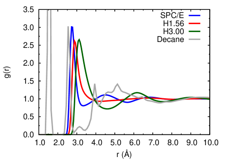
Figure 2: Comparison of the oxygen-oxygen radial distribution functions (RDFs) for modified hybrid water models with $\lambda$ = 1.00, 1.56 and 3.00 at 300 K and 1 atm. The RDF of decane monomer units including bond, angle and dihedral peaks has also been shown at the same temperature and pressure.

The number densities, $\rho_{liq}^{*}$, reported in Table 1 for different solvents are almost similar ($\approx$ 0.03 $\mathring{A}$ ^-3). The number densities for modified hybrid water models have been calculated by taking the number of oxygen atoms, whereas in case of decane, each decane monomer unit is taken as a single entity. The correlation coefficient ($R={\left<\Delta W\Delta U\right>}/{\sqrt{\left<\left(\Delta W\right)^{2}\right>}\sqrt{\left<\left(\Delta U\right)^{2}\right>}}$) and the slope of the correlation plot ($\gamma_{UW}={\left<\Delta W\Delta U\right>}/{\left<\left(\Delta U\right)^{2}\right>}$) are also reportedBailey et al. (2008a, b); Schrøder et al. (2009); Gnan et al. (2009); Pedersen et al. (2008); Bøhling et al. (2012); Dyre (2013); Bailey et al. (2013). The correlation coefficient defines the correlation between configurational energy and virial for liquids and can be used to judge the extent of simple liquid behaviour. Simple liquids show very strong configurational energy-virial correlations with $R\geq$ 0.90Bailey et al. (2008a). As the $\lambda$ is increased from 1.00 to 3.00, the $R$ value increases from 0.063 to 0.317, indicating a progressive increase in simple liquid behaviour. The slope of the correlation plot also increases from 0.349 for $\lambda$ = 1.00 to 2.768 for $\lambda$ = 3.00. In case of decane, for calculating the correlation coefficient, only non-bonded contributions to potential energy and virial are considered. The $R$ value is very high for decane and this value as well as the corresponding $\gamma_{UW}$ value for decane are comparable to simple liquids. High $R$ values also indicate that the structure and dynamics of the liquid will be dominated by pair correlations. The isothermal compressibilities, pair entropies and diffusivities of different solvents have also been reported in Table 1. The isothermal compressibilities ($\kappa_{\tau}$) are calculated using fluctuation formula and give the extent to which a liquid can be compressed under certain applied pressure. The pair entropy can be related to the local structure of the liquid and for an atomic mixture with $X_{\alpha}$ mole fraction of species $\alpha$, the pair entropy, $S_{2}$, is given by $S_{2}/Nk_{B}=\sum_{\alpha,\beta}X_{\alpha}X_{\beta}S_{\alpha\beta}$,

$$S_{\alpha\beta}=-2\pi\rho\int_{0}^{\infty}\{g_{\alpha\beta}(r)\ln g_{\alpha\beta}(r)-\left[g_{\alpha\beta}(r)-1\right]\}r^{2}dr$$ (12)

where $g_{\alpha\beta}(r)$ is the pair correlation function (PCF) between atoms of type $\alpha$ and $\beta$Hernando (1990); Laird and Haymet (1992). The diffusivities were calculated using the Einstein relation ($D_{\alpha}=\lim_{t\rightarrow\infty}{\langle|\delta{\bf{r}}_{i}\left(t\right)|^{2}\rangle}/{6t}$)Hansen and McDonald (2006). Decane has the highest compressibility with lowest entropy and diffusivity among all the solvents used at 300 K and 1 atm, whereas if we consider modified hybrid water models, the compressibility, pair entropy and diffusivity follow non-monotonic behaviour with the increase in hybrid potential parameter, $\lambda$. The non-monotonic changes observed in different thermodynamic and dynamic properties of modified hybrid water models are in sync with the changes observed in the structure defined by radial distribution functions as shown in Figure 2. The liquid with intermediate $\lambda$ value (H1.56), has the least structure beyond the first shell and is evident from high compressibility, pair entropy and diffusivity values as compared to other modified hybrid water models. In our earlier paper on modified hybrid water models, we have reported the change in LJ and electrostatic contributions to the configurational energy with the change in $\lambda$Prasad and Chakravarty (2014). With the increase in $\lambda$, the LJ contribution to configurational energy becomes more negative and the electrostatic contribution becomes more positivePrasad and Chakravarty (2014). For H3.00, the electrostatic contribution to the configurational energy is dominant (but more positive as compared to SPC/E and H1.56) and the hydrogen-bond energy is estimated to be 70$\%$ of the value for SPC/E water. Therefore, the system can be treated as a moderately polar one.

Table 1: The structure, thermodynamic and dynamic properties of all the solvents used in this study at 300 K and 1 atm. The number density ($\rho^{*}_{liq}$), correlation coefficient ($R$), slope of the correlation plot ($\gamma_{UW}$), isothermal compressibility ($\kappa_{\tau}$), pair entropy (S₂/Nk_B) and diffusivity (oxygen of water/decane monomer unit of different solvents) are tabulated.

Solvent	$\rho^{*}_{liq}$ ($\mathring{A}$ -3)	R	$\gamma_{UW}$	$\kappa_{\tau}$ (10-10 Pa-1)	S2/NkB	Diff. (10-9 m2 s-1)
SPC/E	0.033	0.063	0.349	4.521	-2.175	2.853
H1.56	0.032	0.152	0.935	4.677	-2.085	5.835
H3.00	0.032	0.317	1.991	2.768	-2.558	5.512
Decane	0.031	0.911	5.421	13.584	-3.836	2.275

IV.2 Solvation of a Single Nanoparticle

In this section, we study the solvation of three types of end group functionalized nanoparticles in various solvent medium and infer the effects caused due to the reorganization of solvent and ligand in presence of each other.

IV.2.1 Effect of Solvent Reorganization

The reorganization of water molecules and decane monomers around the Au₁₄₀(SC₁₀)₆₂, Au₁₄₀(SC₉NH₂)₆₂ and Au₁₄₀(SC₉COOH)₆₂ nanoparticles can be described by the pair correlation function (PCF), $g_{ns}(r)$. Figure 3(a) shows the pair correlation function for all three types of nanoparticles solvated in water and decane at 300 K and 1 atm.

Figure 3: Pair correlation function, $g_{ns}(r)$: (a) for different end groups functionalized nanoparticles in SPC/E water and decane, (b) for Au₁₄₀(SC₉COOH)₆₂ nanoparticle in different solvents at 300 K and 1 atm.

The end group functionalization of nanoparticles does not seem to have a substantial effect on the arrangement of water molecules, since the PCFs in SPC/E water, show little variation with functionalization, but the solvation properties related to integral of $g_{ns}(r)$ are expected to show significant differences. The $g_{ns}(r)<$ 1.0, even in the soft corona region of the nanoparticles. This is due to the greater solvent-solvent interactions compared to solute-solvent interactions. This type of PCF has already been observed in the literature for solvation of Au₁₄₀(SC₁₀)₆₂ nanoparticle in decane and other organic solvents at very high densities, whereas the solvation of Au₁₄₀(SC₁₀)₆₂ nanoparticle in ethane and propane at lower densities close to critical isotherm show well defined solvation shell ($g_{ns}(r)>$ 1.0)Yadav et al. (2016); Yadav and Chakravarty (2017). Decane solvent shows better penetrability at lower $r$ values compared to water due to the favorable interactions between methylene units of ligand and decane monomer units. In decane, Au₁₄₀(SC₁₀)₆₂ and Au₁₄₀(SC₉NH₂)₆₂ nanoparticles show similar and greater solvent penetration at lower $r$ as compared to Au₁₄₀(SC₉COOH)₆₂ nanoparticle. To understand the penetration effect of solvent, we have also reported the PCFs for Au₁₄₀(SC₉COOH)₆₂ nanoparticle in modified hybrid water solvents where the repulsion-dispersion interaction is enhanced as compared to the electrostatic interaction as shown in Figure 3(b). With the increase in $\lambda$, the repulsion-dispersion contribution to the total potential energy of the solvent increases. The penetrability of the solvent at lower $r$ increases with increase in $\lambda$ and is highest in case of decane, where the solute-solvent interaction is even more favorable compared to H3.00 modified hybrid water model. Similar effects with the change in the solvent can also be seen for Au₁₄₀(SC₁₀)₆₂ and Au₁₄₀(SC₉NH₂)₆₂ nanoparticles (data not shown here).

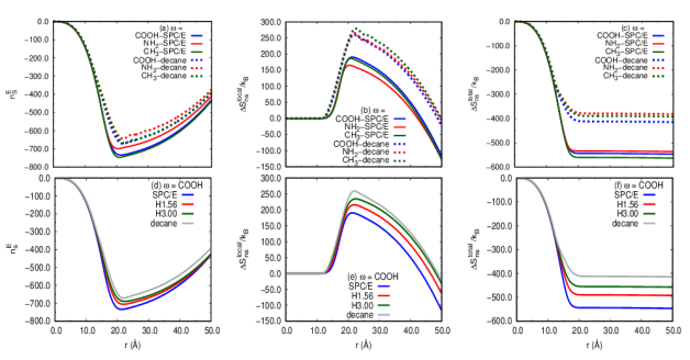
Figure 4: The running integral of different solvation properties: (a) solvent excess number, $n^{E}_{s}$, (b) solvation pair entropy due to local ordering of solvents, ${\Delta}S^{local}_{ns}/k_{B}$ and (d) total entropy of solvation with local and long-range correction terms, ${\Delta}S^{total}_{ns}/k_{B}$, in water and decane at 300 K and 1 atm. (d) $n^{E}_{s}$, (e) ${\Delta}S^{local}_{ns}/k_{B}$ and (f) ${\Delta}S^{total}_{ns}/k_{B}$ for Au₁₄₀(SC₉COOH)₆₂ nanoparticle in different solvents at 300 K and 1 atm.

The reported pair correlation functions, $g_{ns}(r)$, do not approach unity even when $r\,\to\,\infty$ due to use of finite system size and NVT conditions, which results in a significant deviation of $1/N$ from unity. Hence, all the solvation quantities, which depend on the Kirkwood-Buff integral do not converge, however, the relative values can provide significant information.

Figure 4 shows the running integral of the solvation properties for all three types of nanoparticles in water and decane and for Au₁₄₀(SC₉COOH)₆₂ nanoparticle in different solvents at 300 K and 1 atm. It has already been shown in literature that the $n^{E}_{s}$ is positive and shows anti-correlating behavior w.r.t local entropy (${\Delta}S^{local}_{ns}/k_{B}$) for solvation of alkanethiol passivated gold nanoparticle in ethane and propane at low and intermediate densities near the critical isotherm, where well defined solvation shell (g_ns(r) $>$ 1.0) is observedNayar et al. (2012); Yadav and Chakravarty (2017). At very high densities, no well defined solvation shell is observed (g_ns(r) $<$ 1.0), the solvent excess shows negative values and the anti-correlation does not seem to hold true in that caseNayar et al. (2012); Yadav et al. (2016); Yadav and Chakravarty (2017), which is similar to our study. In our study, $n^{E}_{s}$ is maximum (less negative) in decane for all the nanoparticles i.e. the affinity of nanoparticles for decane solvent is highest among all the solvents used in this study, which is expected, since the penetration of decane into the ligand shell is maximum. With the increase in $\lambda$ or repulsion-dispersion interaction, the solvent penetration increases inside the ligand soft corona as compared to H1.00 as seen in Figure 3(b), which gives less negative $n^{E}_{s}$ value in H3.00 than H1.56 and H1.00 i.e., the nanoparticles are better solvated in H3.00 as compared to H1.56 and H1.00. In all the solvents, the $n^{E}_{s}$ value is less negative for Au₁₄₀(SC₉NH₂)₆₂ than Au₁₄₀(SC₁₀)₆₂ and Au₁₄₀(SC₉COOH)₆₂ nanoparticles. Temperature also affects the n${}^{E}_{s}$ value. At lower temperature, the affinity of solute for any solvent is more than at higher temperature (data not shown here).

We have also estimated the local (${\Delta}S^{local}_{ns}/k_{B}$) and total entropy (${\Delta}S^{total}_{ns}/k_{B}$) as shown in Figures 4(b,e), 4(c,f), respectively. The local entropy, as well as the total entropy, is generally maximum in decane even when the solvent penetration inside the ligand shell is maximum for decane. In modified hybrid water models, the local entropy and the total entropy increase with the increase in $\lambda$. A significant part of the variation in total entropy arises due to local entropic contributions.

In order to understand the behaviour of water molecules in the presence of end group functionalized nanoparticles, we attempt to quantify the changes in the local ordering of water molecules by calculating the local tetrahedral order metric, $q_{tet}$. The breakdown of the tetrahedral, hydrogen bond network of water in the presence of different solutes can be best monitored using the local tetrahedral order parameterChau and Hardwick (1998); Errington and Debenedetti (2001); Nayar and Chakravarty (2013); Tanaka (2012). The local tetrahedral order parameter, $q_{tet}$, associated with an atom $i$, is defined as Chau and Hardwick (1998); Errington and Debenedetti (2001)

$$q_{tet,i}=1-\frac{3}{8}\sum_{j=1}^{3}\sum_{k=j+1}^{4}\left(\cos\psi_{jik}+\frac{1}{3}\right)^{2}$$ (13)

where $j,k$ are the nearest neighbors to the central atom, $i$ of a given molecule. $\psi_{jik}$ is the angle formed between the bond vectors ${\bf r}_{ij}$ and ${\bf r}_{ik}$. For perfect tetrahedrality, the value of $q_{tet}$ is 1. While calculating $q_{tet}$, we have considered oxygen atom of water molecules and no other atoms of the passivated nanoparticle. Figure 5 shows the local tetrahedral order of waters, $q_{tet}(r)$, as a function of the distance from the center of mass of the gold core in SPC/E or H1.00 and H3.00 at 275 K and 1 atm, since the effect is more prominent at low temperatures.

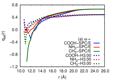
Figure 5: Comparison of the average local tetrahedral order of waters, $q_{tet}(r)$, as a function of the distance from the center of mass of the $Au_{140}$ nano-core in H1.00 or SPC/E and H3.00 at 275 K and 1 atm. Solid and dashed lines are used for nanoparticles solvated in H1.00 and H3.00 modified hybrid water model, respectively.

At very large distances ($r>$ 24 $\mathring{A}$ ) from the center of mass of the gold core, the effects due to the presence of nanoparticles as a solute are insignificant and the tetrahedral order corresponds to the bulk value for SPC/E and H3.00 i.e., 0.664 and 0.485, respectively, at 275 K and 1 atm. The bulk value for SPC/E is high compared to H3.00 because of the differences in the hydrogen bond strengths of the two liquids. $q_{tet}(r)$ decreases only when $r$ is close to the periphery of the passivated nanoparticle. The decrease in $q_{tet}$ with $r$ is more pronounced for SPC/E water compared to H3.00. At low $r$, the decrease is more prominent, probably because of the less number of SPC/E water compared to H3.00 water inside the ligand shell as evident from the degree of penetration of solvents as shown in Figure 3(b). The Au₁₄₀(SC₉COOH)₆₂ nanoparticle affects the tetrahedral ordered network of water to a greater extent as compared to other end group functionalized nanoparticles used in this study as apparent from the $q_{tet}(r)$ data for all other nanoparticles in SPC/E water. This can be well understood by plotting the conditional tetrahedral distribution, $P_{r}(q_{tet})$, plots. Figure 6 shows the conditional tetrahedral distributions, calculated for water molecules lying within distances of 35-36 $\mathring{A}$ , 19-20 $\mathring{A}$ , and 15-16 $\mathring{A}$  from the center of mass of the gold core for SPC/E and H3.00 water at 275 K and 1 atm. For SPC/E water, the $P_{r}(q_{tet})$ plots for all the three end group passivated nanoparticle system at 35-36 $\mathring{A}$  distance overlap with each other and show a high tetrahedrality peak at $\approx$ 0.80 and a very small bump at slightly low tetrahedrality. Thus, there is no effect due to nanoparticles or the end group functionalization on the tetrahedral structure of water molecules and the $q_{tet}(r)$ resembles the tetrahedral order of bulk water. At 19-20 $\mathring{A}$  distance, the water molecules are near or just inside the ligand soft corona and hence the effect due to end group functionalization can be clearly seen. The degree of interaction of the functionalized group with water molecules follows the order COOH $>$ NH₂ $>$ CH₃ and hence the degree of breaking the tetrahedral order of water also follows the same order as noticeable in the $P_{r}(q_{tet})$ plots at intermediate $r$. At this distance, a clear bimodal distribution can be seen. In case of H3.00 modified hybrid water as the solvent, the tetrahedral structure of the liquid is already broken due to low hydrogen bond strength and hence all the $P_{r}(q_{tet})$ plots look alike.

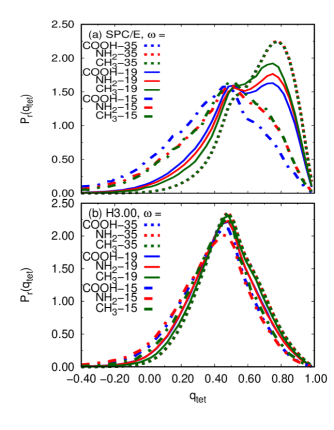
Figure 6: Conditional tetrahedral distributions, $P_{r}(q_{tet})$, calculated for water molecules lying within distances of 35-36 $\mathring{A}$ , 19-20 $\mathring{A}$ , and 15-16 $\mathring{A}$   from the center of mass of the gold core for (a) SPC/E and (b) H3.00 water at 275 K and 1 atm.

IV.2.2 Effect of Ligand Reorganization

In this section, we attempt to quantify the structure of the ligand shell of the three end group functionalized nanoparticles used in this study in the presence of liquids with varying degrees of repulsion-dispersion and electrostatic interactions. The ligands are free to move in the presence of solvent and hence, contribute to the total free energy of solvation. The shape and size of the passivated nanoparticle also affects the self-assembly process. Figure 7(a) shows the structure of the ligand shells, characterized by radial density profiles (RDP), $\rho_{L}(r)$, in SPC/E water and decane at 300 K and 1 atm.

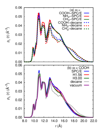
Figure 7: Radial density profiles, $\rho_{L}(r)$, of ligand chain monomers (for nine CH₂ groups only, which are common in all the end group functionalized nanoparticles) in (a) water and decane and (b) solvents of varying degrees of repulsion-dispersion and electrostatic interactions for Au₁₄₀(SC₉COOH)₆₂ nanoparticle at 300 K and 1 atm.

The nine methylene groups, which are common in all type of ligands are used to compute the radial density profiles with respect to the center of mass of the gold core. In SPC/E water, the structures of all the different types of ligand shells are almost similar, except slight differences in peak heights for SC₁₀ ligand shell as compared to SC₉NH₂ and SC₉COOH ligand shells. The similarity of RDPs in SPC/E water may be attributed to very less penetration into the ligand soft corona by water molecules. The ligand structure is more open and stretched in decane compared to SPC/E, probably due to more penetration of decane solvent inside the ligand shell as compared to SPC/E. The methylene units are stretched up to $\approx$ 21 $\mathring{A}$   and $\approx$ 20 $\mathring{A}$  in decane and SPC/E, respectively. The differences between the structure of different ligand shells are also more prominent in decane than SPC/E. Figure 7(b) shows the SC₉COOH ligand shell structure in different solvents and vacuum. As we have already mentioned, with the increase in interaction between solute methylene units and solvent, the penetration of the solvent inside the ligand shell increases. This increase affects the ligand shell structure and the ligands try to stretch more, which increases the probability of methylene units at $r>$ 16 $\mathring{A}$   and decreases the probability of methylene units at intermediate $r$ values from the center of mass of the gold core.

In order to quantify the structure of the ligand shell further, we have calculated the radius of gyration ($R_{g}$), which provides a quantitative measure of the expanded state of the ligand shell and we attempt to relate the $R_{g}$ data to the RDPs and the inherent anisotropy of the passivated nanoparticles. $R_{g}$ has been calculated using the average distances of sulfur and methylene groups of all the ligand chains from the center of mass of the gold core and are reported in Figure 8(a). Since all three types of ligand shells are most stretched in decane solvent, as apparent from Figure 7, the highest $R_{g}$ value for all three types of ligands is seen in decane solvent. The $R_{g}$ values follow the order, decane $>$ vacuum $>$ H3.00 $\approx$ H1.56 $>$ SPC/E. The $R_{g}$ value for SC₉COOH ligand shell is in general slightly less as compared to SC₉NH₂ and SC₁₀ ligand shells except in vacuum, probably because the COOH group is a bulky group compared to CH₃, NH₂ groups and under the effect of this bulky group and pressure of the solvent, the ligand chains fold slightly. Temperature also significantly alters the $R_{g}$ values, but this effect cannot be generalized.

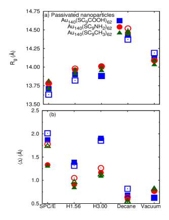
Figure 8: (a) Radius of gyration between the center of mass of the gold nano-core and the SH, CH₂ groups of the passivating ligands and (b) $\langle\Delta\rangle$, where, $\Delta$, denotes the magnitude of the vector connecting the center of mass of the gold nano-core and the SH, CH₂ groups of the ligand shell. The solid and open points are used for data at 300 and 275 K at 1 atm, respectively.

Figure 8(b) shows the $\langle\Delta\rangle$, where $\Delta$ denotes the magnitude of the vector connecting the center of mass of the gold core and the sulfur and methylene groups of the ligand shell. The sulfur and methylene groups are considered to effectively compare all the three types of ligand shells. The $\Delta$ value represents the degree of inherent anisotropy present in the passivated nanoparticles, more the $\Delta$ value, more is the anisotropy. The highest anisotropy is seen in SPC/E and H3.00 water and least in decane for all the three types of ligand shells. The anisotropy follows the order, SPC/E $\approx$ H3.00 $>$ H1.56 $>$ vacuum $\approx$ decane, which is almost inverse of the order observed for $R_{g}$. The anisotropy of the ligand shells depend on the competition between different types of interactions such as ligand-solvent interaction, ligand-ligand interaction, the free volume available to each chain and slightly on the mobility of the solvent. In H1.56, the ligand shells show low anisotropy compared to SPC/E may be due to greater ligand-solvent interaction and also due to high diffusivity of H1.56 solvent as given in Table 1. The ligand shells in H3.00 show higher anisotropy compared to H1.56 irrespective of better ligand-solvent interaction as evident from greater solvent penetration and higher solvent excess for H3.00, possibly due to low diffusivity of solvent compared to H1.56. The anisotropy of SC₉COOH ligand shell is generally high in all media studied, except in vacuum, which is also inverse of what we observed in case of $R_{g}$ values. The high values of anisotropy in SC₉COOH ligand shell in SPC/E and modified hybrid water models can be attributed to the formation of ligand-ligand or ligand-solvent hydrogen bonds. At low temperature, generally, the anisotropy increases except in certain cases reported in this study. For a better understanding of the extent of anisotropy, we have also shown the probability distribution of $\Delta$ in Figure S4 of the supplementary materialsup . All the quantities calculated above to quantify the effect of ligand reorganization have taken into account the part of ligands which are common in all ligands, hence even a small change is of importance and will magnify the difference if the entire ligand is taken into account. Figure 9 shows the snapshots of all three types of passivated nanoparticles solvated in different solvent media. The snapshots clearly show the significant qualitative differences in the structure of the coatings or coating asymmetry.

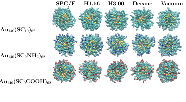
Figure 9: Snapshots of different end group functionalized nanoparticles in solvents of varying interactions at 300 K and 1 atm. Solvent molecules are not shown for clarity. Sulfur atoms are shown in yellow, carbon in cyan, oxygen in red, nitrogen in blue and hydrogen in white.

In Table 2, we have reported the upper bound to the ligand shell configurational entropy using Schlitter’s methodSchlitter (1993). This method was originally developed to calculate the configurational entropy of biomolecules. The soft ligand shell is expected to reorganize differently in different solvent media and the entropy associated with the organization of the ligand shell can be computed using the covariances of fluctuations in positions of ligand atoms. The entropy for all three nanoparticles is maximum in vacuum and follows the order, vacuum $>$ decane $>$ H1.56 $>$ H3.00 $\approx$ SPC/E. Nanoparticles in decane have greater ligand shell configurational entropy than all other water models due to greater penetration of decane solvent into the ligand shell. H3.00 solvent penetrates the ligand shell to a greater extent than H1.56 solvent, but the ligand shell configurational entropy is more in H1.56 compared to H3.00. The H1.56 solvent has significantly greater diffusivity than H3.00 and SPC/E as shown in Table 1. The greater diffusivity contributes to the enhanced reorganization of ligand shell and hence the S_L is more for nanoparticles solvated in H1.56 than H1.00 and H3.00. Therefore, S_L also depends on the local fluctuations of the solvent mediumGupta, Chakravarty, and Bandyopadhyay (2016); Gupta et al. (2016). If we compare the S_L of the three nanoparticles in all the solvents used, we find that S_L of Au₁₄₀(SC₁₀)₆₂  $>$ Au₁₄₀(SC₉NH₂)₆₂  $>$ Au₁₄₀(SC₉COOH)₆₂. The S_L for Au₁₄₀(SC₉COOH)₆₂ is minimum may be due to the formation of hydrogen bonds between the two COOH groups of different ligands of the same nanoparticle, which restricts the ligand motions, when the nanoparticle is solvated in non-polar liquid like decane. The COOH group from the Au₁₄₀(SC₉COOH)₆₂ nanoparticle, when solvated in polar liquid like water is expected to form hydrogen bonds with water, which may also restrict the ligand motions and decreases the ligand shell configurational entropy.

Table 2: Ligand shell configurational entropy, $S_{L}$ (J K^-1 mol^-1), due to the reorganization of the ligands in the presence of different solvents at 300 K and 1 atm.

NP/Solvent	SPC/E	H1.56	H3.00	Decane	Vacuum
Au140(SC10)62	58.98	59.59	58.79	59.90	63.95
Au140(SC9NH2)62	53.81	54.73	54.59	55.56	58.54
Au140(SC9COOH)62	48.50	49.88	49.73	50.37	53.82

IV.3 Effective Interactions Between a Pair of Nanoparticles

In this section, we have computed the isotropic potential of mean force (PMF) between two identical end group functionalized ligand passivated nanoparticles in vacuum, SPC/E water and H3.00 modified hybrid water. The gold nanoparticles self-assemble to form body-centered cubic (bcc), face-centered cubic (fcc) and hexagonal close-packed (hcp) ordered structures depending on the ligand and solvent quality, indicating that the PMF between a pair of nanoparticles is isotropic in nature. However, the gold nanoparticles depending on the ligand, solvent quality and temperature, also form amorphous agglomerates, suggesting the presence of some angular dependence in addition to pair separation distance in overall free energy between a pair of nanoparticles. So, we have also characterized the fluctuation driven anisotropy as a function of the distance between the two nanoparticles in order to understand the importance of anisotropy or orientational dependence arising due to ligand corona fluctuations.

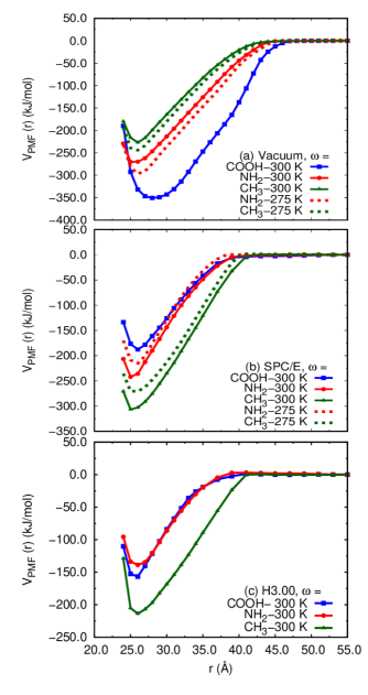
Figure 10: The isotropic potential of mean force, $V_{PMF}(r)$, as a function of pair separation, $r$, between two identical end group functionalized nanoparticles in (a) vacuum, (b) H1.00 or SPC/E and (c) H3.00. Solid lines are for 300 K and dashed lines are for 275 K.

Figure 10 shows the isotropic PMF between two identical nanoparticles (Au₁₄₀(SC₁₀)₆₂ or Au₁₄₀(SC₉NH₂)₆₂ or Au₁₄₀(SC₉COOH)₆₂). In all three media (vacuum, SPC/E water, H3.00 modified hybrid water), the PMF profiles are qualitatively similar and are in contrast to the PMF profile for Au₁₄₀(SC₁₀)₆₂ nanoparticle in organic solvents like hexane, octane and decane as reported in our earlier studyYadav et al. (2016). All the PMF profiles in vacuum, SPC/E and H3.00 are characterized by a deep attractive well, whereas the PMF profile of Au₁₄₀(SC₁₀)₆₂ in organic solvent like decane shows repulsive PMF profile, which indicates that decane acts as a good solvent condition, whereas SPC/E and H3.00 at $\approx$ 1.0 g/cm³ density represent poor solvent conditions as compared to decane. The range of interactions is defined as the maximum pair separation for which the attractive interactions become observable and it can be approximated by $2R_{c}+2L$, where $R_{c}$ is the radius of gold core (8 $\mathring{A}$ ) and $L$ is the distance from the surface of the gold core to a position in space, where the ligand monomer density is effectively zero. The $L$ value can also be approximated using the extended length ($L_{ext}$) of an alkylthiol, $L_{ext}=(n+1)\times 1.2$, where $n$ is the number of carbon atoms in the alkylthiol. The range of interactions is slightly high in vacuum than the approximated value of $2R_{c}+2L\approx$ 42.4 $\mathring{A}$  for Au₁₄₀(SC₁₀)₆₂ nanoparticle, but in solvent, it fits well with the approximated value. All the PMF profiles can be fitted to a Morse function, $D_{e}\left(\left(1-exp\left(-a\left(r-r_{e}\right)\right)\right)^{2}-1\right)$, where $a=\alpha/r_{e}$, $\alpha$ is the dimensionless range parameter, $r_{e}$ is the equilibrium pair separation and $D_{e}$ is the well depth at $r_{e}$. The fitting parameters are reported in Table 3. The attractive well indicates that the energetics due to ligand-ligand interactions dominate over the entropic effect due to interdigitation of ligands. In vacuum, the well depth ($D_{e}$) is maximum and minimum for Au₁₄₀(SC₉COOH)₆₂ and Au₁₄₀(SC₁₀)₆₂ nanoparticle, respectively, since in the absence of solvent, ligand-ligand energetic interaction for SC₉COOH ligands is more as compared to SC₁₀ ligands. In SPC/E water, the variation of well depth follows the reverse order as in vacuum. The well depth for Au₁₄₀(SC₁₀)₆₂ nanoparticle is maximum and minimum for Au₁₄₀(SC₉COOH)₆₂ nanoparticle solvated in SPC/E. This can be explained on the basis of greater COOH-water than CH₃-water interactions. So, the ligand-ligand energetic interaction is more for Au₁₄₀(SC₁₀)₆₂ nanoparticle in SPC/E, which increases the attractive well depth as compared to Au₁₄₀(SC₉COOH)₆₂ nanoparticle. The well depths for all types of nanoparticles are less in H3.00 solvent due to more solvent penetration into ligand shell i.e., better ligand-solvent interaction, which decreases the energetic effect and increases the entropic effect due to ligands. As discussed earlier in case of solvation of single nanoparticle, the solvent penetration into ligand shell is maximum for decane i.e. the ligand-solvent interaction is further enhanced than H3.00 and hence, the PMF profile of Au₁₄₀(SC₁₀)₆₂  in decane is repulsive in nature. The equilibrium separations $r_{e}$ are also quite different in vacuum, but the variation in $r_{e}$ is comparatively less in solvent media as compared to vacuum.

Table 3: The summary of fitting parameters for $V_{PMFs}$ at 300 K. The isotropic PMFs ($V_{PMFs}$) in vacuum as well as in solvents are fitted with Morse function,$D_{e}\left(\left(1-exp\left(-a\left(r-r_{e}\right)\right)\right)^{2}-1\right)$, where $a=\alpha/r_{e}$, $r_{e}$ is the equilibrium pair separation and $D_{e}$ is the well depth at $r_{e}$.

NP/Solvent	Vacuum			SPC/E			H3.00
	De	$a$	re	De	$a$	re	De	$a$	re
	(kJ mol-1)	($\mathring{A}$ -1)	($\mathring{A}$ )	(kJ mol-1)	($\mathring{A}$ -1)	($\mathring{A}$ )	(kJ mol-1)	($\mathring{A}$ -1)	($\mathring{A}$ )
Au140(SC10)62	224.70	0.185	26.01	308.60	0.169	25.60	209.20	0.165	26.22
Au140(SC9NH2)62	271.00	0.155	25.85	243.60	0.240	25.48	140.80	0.247	25.81
Au140(SC9COOH)62	358.30	0.130	27.84	191.70	0.238	25.99	159.70	0.284	25.65

To understand the effect of the thermodynamic variable like temperature, we have also reported the isotropic PMFs for CH₃ and NH₂ functionalized nanoparticles in vacuum and water at 275 K in Figures 10(a) and 10(b), respectively. We find that in case of vacuum, with the decrease in temperature, the attractive well-depth increases for both CH₃ and NH₂ functionalized nanoparticles, whereas in water, the well-depth decreases with the decrease in temperature for both CH₃ and NH₂ functionalized nanoparticles, which is in contrast to vacuum results.

Figure 11 shows snapshots of a pair of Au₁₄₀(SC₉COOH)₆₂ nanoparticles at different inter-nanoparticle pair separations, $r$, in vacuum and SPC/E water. When the two nanoparticles are at very large separation (55 $\mathring{A}$ ), the fluctuations in the ligand shell give rise to inherent anisotropy. The inherent anisotropy of all the nanoparticles including Au₁₄₀(SC₉COOH)₆₂ is more in SPC/E than in vacuum as can be seen clearly in Figure 8(b). At $r$ = 55 $\mathring{A}$  distance, there is almost negligible interaction between the two NPs, but as the pair separation is decreased, the interaction between the nanoparticles increases, giving rise to emergent anisotropy.

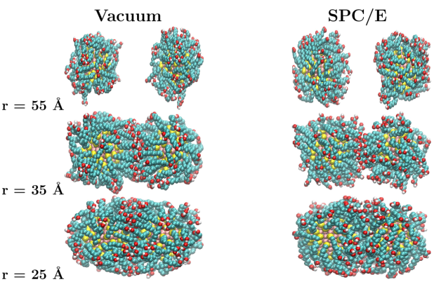
Figure 11: Anisotropy due to ligand shell disorder at different pair separations for the Au₁₄₀(SC₉COOH)₆₂ nanoparticle in vacuum and SPC/E water at 300 K. The color coding is same as in Figure 9.

In vacuum, due to the absence of ligand-solvent interaction, the ligand-ligand interaction is more compared to SPC/E and hence greater number of ligands align in the direction of the inter-nanoparticle axis compared to SPC/E as can be seen at $r$ = 35 $\mathring{A}$  in Figure 11. With the further decrease in the pair separation, the ligands are pushed out from the space between the two nanoparticles.

Figure 12 shows the change in the average mass dipole ($\langle\Delta\rangle$) and the orientation of the mass dipole vector, characterized by the cosine of the angle ($\cos\theta$) between the mass dipole vector and the inter-nanoparticle axis with the change in the pair separation between the two nanoparticles. The higher average mass dipole value indicates higher asymmetry. The value of $\langle\cos~{}\theta\rangle$ can vary from -1 to 1. The $\langle\Delta\rangle$ value for a pair of nanoparticles of all three types do not change much up to $\approx$ 45 $\mathring{A}$   in vacuum, which is close to $2R_{c}+2L$ value. With the further decrease in pair separation, the $\langle\Delta\rangle$ increases up to $r\approx$ 33 $\mathring{A}$ , which is close to $2R_{c}+L$ value due to attractive energetic interactions between ligands as shown by an attractive well in $V_{PMF}$ profiles (see Figure 10). With the further decrease in pair separation, the $\langle\Delta\rangle$ decreases as the ligands are pushed out of the inter-nanoparticle space due to the entropic repulsion of ligands as characterized by the increase in the value of $V_{PMF}$. The increase is maximum for Au₁₄₀(SC₉COOH)₆₂ nanoparticle and minimum for Au₁₄₀(SC₁₀)₆₂ nanoparticle. The change in the $\langle\Delta\rangle$ is the result of the changes in the orientation of the ligands due to decreasing pair separation between the nanoparticles. The $\langle\cos~{}\theta\rangle$ shows qualitatively similar behaviour as of the $\langle\Delta\rangle$. At large separation, the $\langle\cos~{}\theta\rangle$ is close to zero and does not change much up to $\approx$ 45 $\mathring{A}$ , with further decrease in pair separation, the $\langle\cos~{}\theta\rangle$ shows values close to 1.0 due to the alignment of ligands in the same direction to the inter-nanoparticle axis. At very low pair separations, the ligands are pushed out from the inter-nanoparticle space due to entropic repulsion between ligand atoms and the $\langle\cos~{}\theta\rangle$ shows lower values.

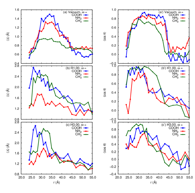
Figure 12: Fluctuation-driven anisotropy in passivated nanoparticles as a function of pair separation, $r$, at 300 K. The mean value of the magnitude of the mass dipole, $\langle\Delta\rangle$, and the mean angle between the mass dipole vector and the inter-nanoparticle axis, $\langle\cos~{}\theta\rangle$, are shown in (a and a^′) vacuum, (b and b^′) H1.00 or SPC/E and (c and c^′) H3.00, respectively.

In vacuum, the $\langle\Delta\rangle$ is relatively low at all pair separations compared to $\langle\Delta\rangle$ values in SPC/E and H3.00 may be due to higher inherent anisotropy observed for all single nanoparticles in these solvents. In SPC/E and H3.00 solvents, the Au₁₄₀(SC₁₀)₆₂ nanoparticle shows greater emergent anisotropy compared to Au₁₄₀(SC₉NH₂)₆₂ and Au₁₄₀(SC₉COOH)₆₂ nanoparticles at lower pair separations, which is in agreement with the lower well depth value observed in $V_{PMF}$ profiles in these solvents for Au₁₄₀(SC₁₀)₆₂ nanoparticle. The emergent anisotropy in solvents is maximum at very low pair separations, whereas in vacuum, the emergent anisotropy is maximum at intermediate pair separations between the two nanoparticles.

V Conclusions

This study examines the solvation behaviour of end group functionalized alkylthiols passivated gold nanoparticles namely Au₁₄₀(SC₁₀)₆₂, Au₁₄₀(SC₉NH₂)₆₂ and
Au₁₄₀(SC₉COOH)₆₂ in solvents with varying degrees of repulsion-dispersion and electrostatic interactions. The solvent reorganization around the end group functionalized nanoparticles are characterized by the pair correlation functions, $g_{ns}(r)$, between the center of mass of the gold nano-core and solvent atoms. The PCFs of functionalized nanoparticles in SPC/E water show only slight differences, but the solvation properties calculated using, $g_{ns}(r)$, show significant differences. As the repulsion-dispersion interactions are enhanced relative to the electrostatic interactions, the solvent penetrability inside the ligand soft corona increases at lower $r$. Decane solvent shows maximum penetrability, even higher than H3.00 modified hybrid water. $g_{ns}(r)<$ 1.0, in the ligand soft corona for combinations of all types of nanoparticles and solvents, due to greater solvent-solvent interactions compared to solute-solvent interactions. The solvent excess, $n^{E}_{s}$, is maximum (less negative) in decane and minimum (more negative) in H1.00. It gives the quantitative measure of the affinity of solute particle for a given solvent, hence the affinity of nanoparticles for decane solvent is highest among all the solvents used in this study. At lower temperature, solute-solvent interaction is relatively high as indicated by less negative value of $n^{E}_{s}$. The local entropy ($\Delta S^{loc}_{ns}$) and total entropy ($\Delta S^{tot}_{ns}$) increase with increase in repulsion-dispersion interaction of modified hybrid water models, but it is maximum in decane.

The changes in the local structure of water molecules in the presence of end group functionalized nanoparticles is examined using the local tetrahedral order metric, $q_{tet}$. At large $r$ from the center of mass of the nano-core, the effect due to nanoparticles is negligible, even for Au₁₄₀(SC₉COOH)₆₂ nanoparticle. At the periphery of the passivated nanoparticle, changes in the local structure of water molecules are eminent. The change is maximum for Au₁₄₀(SC₉COOH)₆₂ nanoparticle as evident from both $q_{tet}(r)$ and $P_{r}(q_{tet})$ plots. The degree of breaking the tetrahedral structure of water molecules follow the order Au₁₄₀(SC₉COOH)₆₂ $>$ Au₁₄₀(SC₉NH₂)₆₂ $>$ Au₁₄₀(SC₁₀)₆₂.

The structure of ligands are characterized using the radial density profiles, the radius of gyration ($R_{g}$) and ligand asymmetry parameter ($\langle\Delta\rangle$). The ligands are more open and stretched in decane than water models, probably due to more penetration of decane solvent inside the ligand shell. The effect of functionalization is also more evident in decane than SPC/E water. The $R_{g}$ values support the observations obtained from radial density profiles and follow the order, decane $>$ vacuum $>$ H3.00 $\approx$ H1.56 $>$ SPC/E. The highest anisotropy is seen in SPC/E and H3.00 water and least in decane. The anisotropy is maximum for Au₁₄₀(SC₉COOH)₆₂ nanoparticle compared to Au₁₄₀(SC₁₀)₆₂ and Au₁₄₀(SC₉NH₂)₆₂ nanoparticles in all solvents, except in vacuum. The ligand shell configurational entropy ($S_{L}$) computed using the covariances in particle displacement of ligand atoms for all three nanoparticles follow the order, vacuum $>$ decane $>$ H1.56 $>$ H3.00 $\approx$ SPC/E. In all solvents, the $S_{L}$ follows the order Au₁₄₀(SC₁₀)₆₂ $>$ Au₁₄₀(SC₉NH₂)₆₂ $>$ Au₁₄₀(SC₉COOH)₆₂.

All the isotropic PMFs for identical nanoparticles in SPC/E and H3.00 water obtained in this study are characterized by a deep attractive well similar to PMF profiles in vacuum. The PMF profiles in SPC/E and H3.00 solvent are in contrast with the repulsive PMF profile of Au₁₄₀(SC₁₀)₆₂ nanoparticle in decaneYadav et al. (2016). This indicates that SPC/E and H3.00 water at density $\approx$ 1.0 g/cm³ act as poor solvent conditions as compared to decane. All the PMF profiles reported in this study are fitted with a Morse function. The well depth, range parameter and the equilibrium separation are significantly different for different nanoparticles in different solvents. In vacuum, the well depth of Au₁₄₀(SC₉COOH)₆₂ nanoparticle is maximum and minimum for Au₁₄₀(SC₁₀)₆₂ nanoparticle, but it is reverse in SPC/E water. The well depths for all nanoparticles are minimum in H3.00 water compared to vacuum and SPC/E water. The equilibrium separations, $r_{e}$, are also quite different in vacuum, but the variations are less in solvent media. The variations arise due to differences in ligand-ligand energetic interaction and entropic effect due to ligands in different solvents. The average mass dipole increases with the decrease in pair separation between nanoparticles and is maximum in the region of attractive $V_{PMF}$. It decreases, when the ligands are pushed out of the inter-nanoparticle space due to entropic repulsion between ligands. Similarly, the orientation of the mass dipole w.r.t inter-nanoparticle axis, characterized by $\langle\cos\theta\rangle$, shows value close to 1.0 in the region of attractive $V_{PMF}$, due to the alignment of ligands in the same direction to the inter-nanoparticle axis. It is interesting to compare the emergent anisotropy results obtained in this study with our previous study of Au₁₄₀(SC₁₀)₆₂  nanoparticle in decane. The $V_{PMF}$ for Au₁₄₀(SC₁₀)₆₂  in decane solvent is repulsive in nature and in the repulsive regime the $\langle\Delta\rangle$ increases significantly accompanied with a sharp decrease in $\langle\cos~{}\theta\rangle$Yadav et al. (2016).

Our results indicate that the chemistry of the ligand and the solvent plays an important role in controlling the solvation and aggregation behavior of the nanoparticles. The structure of the coatings is also highly dependent on the functionalization of passivating ligands and interactions present in the solvent. The changes in the PMF profiles with increasing repulsion-dispersion interaction of solvent signify the importance of solvent chemistry in self-assembly process. It would be interesting to compare our PMF results with PMF profiles for charged end group functionalized ligand passivated nanoparticles in water.

Acknowledgments

The authors are thankful to the Department of Science and Technology, India for financial support. S.P. thanks the University Grants Commission for support through a Senior Research Fellowship. Authors also thank the IIT Delhi HPC facility for computational resources.

References

- Nie, Petukhova, and Kumacheva (2010) Z. Nie, A. Petukhova, and E. Kumacheva, Nat. Nanotechnol. 5, 15 (2010).
- Daniel and Astruc (2004) M.-C. Daniel and D. Astruc, Chem. Rev. 104, 293 (2004).
- Bishop et al. (2009) K. J. M. Bishop, C. E. Wilmer, S. Soh, and B. A. Grzybowski, Small 5, 1600 (2009).
- Walker et al. (2011) D. A. Walker, B. Kowalczyk, M. O. de la Cruz, and B. A. Grzybowski, Nanoscale 3, 1316 (2011).
- Ung, Liz-Marzan, and Mulaveny (2001) T. Ung, L. M. Liz-Marzan, and P. Mulaveny, J. Phys. Chem. B 105, 3441 (2001).
- Tang et al. (1994) H. Tang, K. Prasad, R. Sanjines, P. E. Schmid, and F. Levy, J. Appl. Phys. 75, 2042 (1994).
- Balazs, Emrick, and Russell (2006) A. C. Balazs, T. Emrick, and T. P. Russell, Science 314, 1107 (2006).
- Fu et al. (2008) S.-Y. Fu, X.-Q. Feng, B. Lauke, and Y.-W. Mai, Composites Part B. 39, 933 (2008).
- Wu et al. (2002) C. L. Wu, M. Q. Zhang, M. Z. Rong, and K. Friedrich, Compos. Sci. Technol. 62, 1327 (2002).
- Eastman et al. (2001) J. A. Eastman, S. U. S. Choi, S. Li, W. Yu, and L. J. Thompson, Appl. Phys. Lett. 78, 718 (2001).
- Wang, Xu, and Choi (1999) X. Wang, X. Xu, and S. U. S. Choi, J. Thermophys. Heat Transfer 13, 474 (1999).
- Tang, Kotov, and Giersig (2002) Z. Tang, N. A. Kotov, and M. Giersig, Science 297, 237 (2002).
- Kiely et al. (1998) C. J. Kiely, J. Fink, M. Brust, D. Bethell, and D. J. Schiffrin, Nature 396, 444 (1998).
- Murray, Kagan, and Bawendi (2000) C. B. Murray, C. R. Kagan, and M. G. Bawendi, Annu. Rev. Mater. Sci. 30, 545 (2000).
- Murray, Kagan, and Bawendi (1995) C. B. Murray, C. R. Kagan, and M. G. Bawendi, Science 270, 1335 (1995).
- Shevchenko et al. (2006) E. V. Shevchenko, D. V. Talapin, N. A. Kotov, S. O’Brien, and C. B. Murray, Nature 439, 55 (2006).
- Talapin et al. (2009) D. V. Talapin, E. V. Shevchenko, M. I. Bodnarchuk, X. Ye, J. Chen, and C. B. Murray, Nature 461, 964 (2009).
- Li, Schnablegger, and Mann (1999) M. Li, H. Schnablegger, and S. Mann, Nature 402, 393 (1999).
- Tang et al. (2006) Z. Tang, Z. Zhang, Y. Wang, S. C. Glotzer, and N. A. Kotov, Science 314, 274 (2006).
- Zhang et al. (2006) H. Zhang, E. W. Edwards, D. Wang, and H. Möhwald, Phys. Chem. Chem. Phys. 8, 3288 (2006).
- Min et al. (2008) Y. Min, M. Akbulut, K. Kristiansen, Y. Golan, and J. Israelachvili, Nature Mat. 7, 527 (2008).
- Park et al. (2007) J. Park, J. Joo, S. G. Kwon, Y. Jang, and T. Hyeon, Angew. Chem. Int. Edit. 46, 4630 (2007).
- Lane and Grest (2010) J. M. D. Lane and G. S. Grest, Phys. Rev. Lett. 104, 235501 (2010).
- Luedtke and Landman (1998) W. D. Luedtke and U. Landman, J. Phys. Chem. B 102, 6566 (1998).
- DeLong et al. (2010) R. K. DeLong, C. M. Reynolds, Y. Malcolm, A. Shaeffer, T. Severs, and A. Wanekaya, Nanotechnol., Sci. Appl. 3, 53 (2010).
- He et al. (2011a) J. He, X.-M. Lin, R. Divan, and H. M. Jaeger, Small 7, 3487 (2011a).
- He et al. (2011b) J. He, X.-M. Lin, R. Divan, and H. M. Jaeger, Nano Lett. 11, 2430 (2011b).
- Elghanian et al. (1997) R. Elghanian, J. J. Storhoff, R. C. Mucic, R. L. Letsinger, and C. A. Mirkin, Science 277, 1078 (1997).
- Boisselier and Astruc (2009) E. Boisselier and D. Astruc, Chem. Soc. Rev. 38, 1759 (2009).
- Ghosh et al. (2008) P. Ghosh, G. Han, M. De, C. K. Kim, and V. M. Rotello, Adv. Drug Delivery Rev. 60, 1307 (2008).
- Kalsin et al. (2006) A. M. Kalsin, M. Fialkowski, M. Paszewski, S. K. Smoukov, K. J. M. Bishop, and B. A. Grzybowski, Science 312, 420 (2006).
- Bishop, Chevalier, and Grzybowski (2013) K. J. M. Bishop, N. R. Chevalier, and B. A. Grzybowski, J. Phys. Chem. Lett. 4, 1507 (2013).
- Luedtke and Landman (1996) W. D. Luedtke and U. Landman, J. Phys. Chem 100, 13323 (1996).
- Tay and Bresme (2005) K. Tay and F. Bresme, Mol. Simul. 31, 515 (2005).
- Tay and Bresme (2006) K. A. Tay and F. Bresme, J. Am. Chem. Soc. 128, 14166 (2006).
- Rapino and Zerbetto (2007) S. Rapino and F. Zerbetto, Small 3, 386 (2007).
- Ghorai and Glotzer (2007) P. K. Ghorai and S. C. Glotzer, J. Phys. Chem. C 111, 15857 (2007).
- Singh et al. (2007) C. Singh, P. K. Ghorai, M. A. Horsch, A. M. Jackson, R. G. Larson, F. Stellacci, and S. C. Glotzer, Phys. Rev. Lett. 99, 226106 (2007).
- Schapotschnikow, Pool, and Vlugt (2008) P. Schapotschnikow, R. Pool, and T. J. H. Vlugt, Nano Lett. 8, 2930 (2008).
- Djebaili et al. (2013) T. Djebaili, J. Richardi, A. Stephane, and M. Marchi, J. Phys. Chem. C 117, 17791 (2013).
- Lane and Grest (2014) J. M. D. Lane and G. S. Grest, Nanoscale 6, 5132 (2014).
- Yang, Weng, and Chen (2011) A.-C. Yang, C.-I. Weng, and T.-C. Chen, J. Chem. Phys. 135, 034101 (2011).
- Bolintineanu, Lane, and Grest (2014) D. S. Bolintineanu, J. M. D. Lane, and G. S. Grest, Langmuir 30, 11075 (2014).
- Henz et al. (2011) B. J. Henz, P. W. Chung, J. W. Andzelm, T. L. Chantawansri, J. L. Lenhart, and F. L. Beyer, Langmuir 27, 7836 (2011).
- Heikkila et al. (2012) E. Heikkila, A. Gurtovenko, H. Martinez-Seara, H. Hakkinen, I. Vattulainen, and J. Akola, J. Phys. Chem. C 116, 9805 (2012).
- Giri and Spohr (2015) A. K. Giri and E. Spohr, J. Phys. Chem. C 119, 25566 (2015).
- Lehn and Alexander-katz (2013) R. C. V. Lehn and A. Alexander-katz, J. Phys. Chem. C 117, 20104 (2013).
- Berendsen, Grigera, and Straatsma (1987) H. J. C. Berendsen, J. R. Grigera, and T. P. Straatsma, J. Phys. Chem 91, 6269 (1987).
- Lynden-Bell and Debenedetti (2005) R. M. Lynden-Bell and P. G. Debenedetti, J. Phys. Chem. B 109, 6527 (2005).
- Mishima and Stanley (1998) O. Mishima and H. E. Stanley, Nature 396, 329 (1998).
- Lynden-Bell and Head-Gordon (2006) R. M. Lynden-Bell and T. Head-Gordon, Mol. Phys. 104, 3593 (2006).
- Alejandre and Lynden-Bell (2007) J. Alejandre and R. M. Lynden-Bell, Mol. Phys. 105, 3029 (2007).
- Chatterjee et al. (2008) S. Chatterjee, P. G. Debenedetti, F. H. Stillinger, and R. M. Lynden-Bell, J. Chem. Phys. 128, 124511 (2008).
- Lynden-Bell (2010) R. M. Lynden-Bell, J. Phys.: Condens. Matter 22, 284107 (2010).
- Prasad and Chakravarty (2014) S. Prasad and C. Chakravarty, J. Chem. Phys. 140, 164501 (2014).
- Ben-Naim (1978) A. Ben-Naim, J. Phys. Chem 82, 792 (1978).
- Nayar et al. (2012) D. Nayar, H. O. S. Yadav, B. S. Jabes, and C. Chakravarty, J. Phys. Chem. B 116, 13124 (2012).
- Kirkwood and Buff (1951) J. G. Kirkwood and F. P. Buff, J. Chem. Phys. 19, 774 (1951).
- Lal, Plummer, and Smith (2006) M. Lal, M. Plummer, and W. Smith, J. Phys. Chem. B 110, 20879 (2006).
- Petsche and Debenedetti (1989) I. B. Petsche and P. G. Debenedetti, J. Chem. Phys. 91, 7075 (1989).
- Debenedetti and Mohamed (1989) P. G. Debenedetti and R. S. Mohamed, J. Chem. Phys. 90, 4528 (1989).
- Schlitter (1993) J. Schlitter, Chem. Phys. Lett. 215, 617 (1993).
- Lazaridis (1998a) T. Lazaridis, J. Phys. Chem. B 102, 3531 (1998a).
- Lazaridis (1998b) T. Lazaridis, J. Phys. Chem. B 102, 3542 (1998b).
- Salerno et al. (2014) K. M. Salerno, A. E. Ismail, J. M. D. Lane, and G. S. Grest, J. Chem. Phys. 140, 194904 (2014).
- Bozorgui et al. (2013) B. Bozorgui, D. Meng, S. K. Kumar, C. Chakravarty, and A. Cacciuto, Nano Lett. 13, 2732 (2013).
- Jabes et al. (2014) B. S. Jabes, H. O. S. Yadav, S. K. Kumar, and C. Chakravarty, J. Chem. Phys. 141, 154904 (2014).
- Yadav et al. (2016) H. O. S. Yadav, G. Shrivastav, M. Agarwal, and C. Chakravarty, J. Chem. Phys. 144, 244901 (2016).
- Trzesniak, Kunz, and Gunsteren (2007) D. Trzesniak, A.-P. E. Kunz, and W. F. v. Gunsteren, ChemPhysChem 8, 162 (2007).
- Li et al. (2007) J.-L. Li, R. Car, C. Tang, and N. S. Wingreen, Proc. Natl. Acad. Sci. 104, 2626 (2007).
- Patel and Egorov (2007) N. Patel and S. A. Egorov, J. Chem. Phys. 126, 054706 (2007).
- Yadav and Chakravarty (2017) H. O. S. Yadav and C. Chakravarty, J. Chem. Phys. 146, 174902 (2017).
- (73) See Supplementary Material at for potential parameters of non-bonded, bonded, angle and dihedral interactions.
- koishi and Tamaki (2005) T. koishi and S. Tamaki, J. Chem. Phys. 123, 194501 (2005).
- Landman and Luedtke (2004) U. Landman and W. D. Luedtke, Faraday Discuss. 125, 1 (2004).
- Rizzo and Jorgensen (1999) R. C. Rizzo and W. L. Jorgensen, J. Am. Chem. Soc. 121, 4827 (1999).
- Wick et al. (2005) C. D. Wick, J. M. Stubbs, N. Rai, and J. I. Siepmann, J. Phys. Chem. B 109, 18974 (2005).
- Kamath, Cao, and Potoff (2004) G. Kamath, F. Cao, and J. J. Potoff, J. Phys. Chem. B 108, 14130 (2004).
- Clifford, Bolton, and Ramjugernath (2006) S. Clifford, K. Bolton, and D. Ramjugernath, J. Phys. Chem. B 110, 21938 (2006).
- Leach (1996) A. R. Leach, Molecular Modelling: Princliples and Applications (Addison Wesley Longman, England, 1996).
- Plimpton (1995) S. J. Plimpton, J. Comput. Phys. 117, 1 (1995).
- Martínez et al. (2009) L. Martínez, R. Andrade, E. G. Birgin, and J. M. Martínez, J. Comput. Chem. 30, 2157 (2009).
- Humphrey, Dalke, and Schulten (1996) W. Humphrey, A. Dalke, and K. Schulten, J. Mol. Graphics 14, 33 (1996).
- Bailey et al. (2008a) N. P. Bailey, U. R. Pedersen, N. Gnan, T. B. Schrøder, and J. C. Dyre, J. Chem. Phys. 129, 184507 (2008a).
- Bailey et al. (2008b) N. P. Bailey, U. R. Pedersen, N. Gnan, T. B. Schrøder, and J. C. Dyre, J. Chem. Phys. 129, 184508 (2008b).
- Schrøder et al. (2009) T. B. Schrøder, N. P. Bailey, U. R. Pedersen, N. Gnan, and J. C. Dyre, J. Chem. Phys. 131, 234503 (2009).
- Gnan et al. (2009) N. Gnan, T. B. Schrøder, U. R. Pedersen, N. P. Bailey, and J. C. Dyre, J. Chem. Phys. 131, 234504 (2009).
- Pedersen et al. (2008) U. R. Pedersen, N. P. Bailey, T. B. Schrøder, and J. C. Dyre, Phys. Rev. Lett. 100, 015701 (2008).
- Bøhling et al. (2012) L. Bøhling, T. S. Ingebrigtsen, A. Grzybowski, M. Paluch, J. C. Dyre, and T. B. Schrøder, New J. Phys. 14, 113035 (2012).
- Dyre (2013) J. C. Dyre, Phys. Rev. E. 87, 022106 (2013).
- Bailey et al. (2013) N. P. Bailey, L. Bøhling, A. A. Veldhorst, T. B. Schrøder, and J. C. Dyre, J. Chem. Phys. 139, 184506 (2013).
- Hernando (1990) J. A. Hernando, Mol. Phys. 69, 319 (1990).
- Laird and Haymet (1992) B. B. Laird and A. D. J. Haymet, Phys. Rev. A 45, 5680 (1992).
- Hansen and McDonald (2006) J.-P. Hansen and I. R. McDonald, Theory of Simple Liquids (Elsevier, New York, 2006).
- Chau and Hardwick (1998) P. L. Chau and A. J. Hardwick, Mol. Phys. 93, 511 (1998).
- Errington and Debenedetti (2001) J. R. Errington and P. G. Debenedetti, Nature 409, 318 (2001).
- Nayar and Chakravarty (2013) D. Nayar and C. Chakravarty, Phys. Chem. Chem. Phys. 15, 14162 (2013).
- Tanaka (2012) H. Tanaka, Eur. Phys. J. E 35, 113 (2012).
- Gupta, Chakravarty, and Bandyopadhyay (2016) M. Gupta, C. Chakravarty, and S. Bandyopadhyay, J. Chem. Theory Comput. 12, 5643 (2016).
- Gupta et al. (2016) M. Gupta, D. Nayar, C. Chakravarty, and S. Bandyopadhyay, Phys. Chem. Chem. Phys. 18, 32796 (2016).