Asymptotics of the principal eigenvalue for a linear time-periodic parabolic operator II: Small diffusion

Abstract.

We investigate the effect of small diffusion on the principal eigenvalues of linear time-periodic parabolic operators with zero Neumann boundary conditions in one dimensional space. The asymptotic behaviors of the principal eigenvalues, as the diffusion coefficients tend to zero, are established for non-degenerate and degenerate spatial-temporally varying environments. A new finding is the dependence of these asymptotic behaviors on the periodic solutions of a specific ordinary differential equation induced by the drift. The proofs are based upon delicate constructions of super/sub-solutions and the applications of comparison principles.

1. Introduction

In this paper, we consider the following linear time-periodic parabolic eigenvalue problem in one dimensional space:

(1.1) $$\begin{cases}\vskip 3.0pt plus 1.0pt minus 1.0pt\partial_{t}\varphi-D\partial_{xx}\varphi-\partial_{x}m\partial_{x}\varphi+V\varphi=\lambda(D)\varphi&\text{in}\,\,(0,1)\times(0,T),\\ \vskip 3.0pt plus 1.0pt minus 1.0pt\partial_{x}\varphi(t,0)=\partial_{x}\varphi(1,t)=0&\text{on}\,\,[0,T],\\ \varphi(x,0)=\varphi(x,T)&\text{on}\,\,(0,1),\end{cases}$$

where $D>0$ represents the diffusion rate, and the functions $m\in C^{2,1}([0,1]\times[0,T])$ and $V\in C([0,1]\times[0,T])$ are assumed to be periodic in $t$ with a common period $T$.

By the Krein-Rutman Theorem, (1.1) admits a simple and real eigenvalue (called principal eigenvalue), denoted by $\lambda(D)$, which corresponds to a positive eigenfunction (called principal eigenfunction) and satisfies $\mathrm{Re}\lambda>\lambda(D)$ for any other eigenvalue $\lambda$ of (1.1); see Proposition 7.2 of [12]. The principal eigenvalue $\lambda(D)$ plays a fundamental role in the study of reaction-diffusion equations and systems in spatio-temporal media, e.g. in the stability analysis for equilibria [3, 4, 12, 14]. Of particular interest is to understand the dependence of $\lambda(D)$ on the parameters [15, 16, 19, 20]. The present paper continues our previous studies in [17, 18] on the principal eigenvalues for time-periodic parabolic operators, where the dependence of $\lambda(D)$ on frequency and advection rate were investigated. Our main goal here is to establish the asymptotic behavior of $\lambda(D)$ as the diffusion rate $D$ tends to zero.

For notational convenience, given any $T$-periodic function $p(x,t)$, we define

$$\hat{p}(x):=\frac{1}{T}\int_{0}^{T}p(x,s)\,\mathrm{d}s\quad\text{ and }\quad p_{+}(x,t):=\max\left\{p(x,t),0\right\},$$

and redefine $\partial_{xx}\hat{m}(0)$ and $\partial_{xx}\hat{m}(1)$ via

(1.2) $$\partial_{xx}\hat{m}(0)=\begin{cases}-\infty&\text{if }\partial_{x}\hat{m}(0^{+})<0,\\ \infty&\text{if }\partial_{x}\hat{m}(0^{+})>0,\end{cases}\quad\text{and}\quad\partial_{xx}\hat{m}(1)=\begin{cases}\infty&\text{if }\partial_{x}\hat{m}(1^{-})<0,\\ -\infty&\text{if }\partial_{x}\hat{m}(1^{-})>0.\end{cases}$$

For the case when $V$ and $\partial_{x}m$ depend upon the space variable alone, i.e. $V(x,t)=V(x)$ and $\partial_{x}m(x,t)=m^{\prime}(x)$, problem (1.1) reduces to the following elliptic eigenvalue problem:

(1.3) $$\begin{cases}\vskip 3.0pt plus 1.0pt minus 1.0pt-D\varphi^{\prime\prime}-m^{\prime}(x)\varphi^{\prime}+V(x)\varphi=\lambda(D)\varphi\ \ &\text{in}\,\,(0,1),\\ \varphi^{\prime}(0)=\varphi^{\prime}(1)=0.\end{cases}$$

This sort of advection-diffusion operator in (1.3) with small diffusion can be regarded as a singular perturbation of the corresponding first order operator [24], and was studied in [11] by the large deviation approach. Therein, the limit of the principal eigenvalue $\lambda(D)$ as $D\to 0$ plays a pivotal role in studying the large time behavior of the trajectories of stochastic systems; see also [7, 10]. Recently the asymptotic behavior of $\lambda(D)$ for problem (1.3) has been considered in [6] for general bounded domains, and their result in particular implies

Theorem 1.1.

[6] Assume $V(x,t)=V(x)$ and $\partial_{x}m(x,t)=m^{\prime}(x)$. Suppose that $m^{\prime}(0)\neq 0$, $m^{\prime}(1)\neq 0$, and all critical points of $m$ are non-degenerate. Then

$$\lim_{D\rightarrow 0}\lambda(D)=\min_{x\in\Sigma\cup\{0,1\}}\left\{V\left(x\right)+[m^{\prime\prime}]_{+}\left(x\right)\right\},$$

where $\Sigma:=\{x\in(0,1):m^{\prime}(x)=0\}$ and $m^{\prime\prime}(0),m^{\prime\prime}(1)$ are defined by (1.2).

We refer to [21] for recent progress on problem (1.3) under general boundary conditions.

Theorem 1.1 indicates that the limit of $\lambda(D)$ relies upon the set of critical points of function $m$ in the elliptic scenario. Turning to the time-periodic parabolic case where $m$ depends on both spatial and temporal variables, it seems reasonable to anticipate that the limit of $\lambda(D)$ will be associated to the curves $x(t)$ satisfying $\partial_{x}m(x(t),t)=0$. This is indeed the case for the limit of the principal eigenvalue with large advection, and we refer to Theorem 1.1 in [18] for further details. However, it turns out that this is generally not true while considering the limit of $\lambda(D)$ as $D$ tends to zero. Instead, the asymptotic behavior of $\lambda(D)$ depends heavily on the periodic solutions of the following ordinary differential equation:

(1.4) $$\begin{cases}\vskip 3.0pt plus 1.0pt minus 1.0pt\dot{P}(t)=-\partial_{x}m\left(P(t),t\right),\\ P(t)=P(t+T).\end{cases}$$

More specifically, our main result can be stated as follows.

Theorem 1.2.

Assume that $\partial_{x}m(0,t)\neq 0$ and $\partial_{x}m(1,t)\neq 0$ for all $t\in[0,T]$. Let $\partial_{xx}\hat{m}(0)$ and $\partial_{xx}\hat{m}(1)$ be defined by (1.2).
(i) If (1.4) has at least one but finite many $T$-periodic solutions, denoted by $\{P_{i}(t)\}_{i=1}^{N}$, satisfying $0<P_{1}(t)<\ldots<P_{N}(t)<1$, and $\partial_{xx}m\left(P_{i}(t),t\right)\neq 0$ for $1\leq i\leq N$ and $t\in[0,T]$, then

$$\lim_{D\rightarrow 0}\lambda(D)=\min_{0\leq i\leq N+1}\left\{\frac{1}{T}\int_{0}^{T}\Big{[}V\left(P_{i}(s),s\right)+[\partial_{xx}m]_{+}\left(P_{i}(s),s\right)\Big{]}\mathrm{d}s\right\},$$

where $P_{0}(t)\equiv 0$ and $P_{N+1}(t)\equiv 1$;

(ii) If (1.4) has no periodic solutions, then

$$\lim_{D\rightarrow 0}\lambda(D)=\min\Big{\{}\hat{V}(0)+[\partial_{xx}\hat{m}]_{+}\left(0\right),\,\,\hat{V}(1)+[\partial_{xx}\hat{m}]_{+}\left(1\right)\Big{\}}.$$

If $V$ and $m$ are independent of time, all solutions of (1.4) are constants which correspond to the critical points of function $m$, and part (i) of Theorem 1.2 is reduced to Theorem 1.1. When $m(x,t)$ is monotone in $x$, part (ii) of Theorem 1.2 was first established in [22].

One potential application of Theorem 1.2 is the study of large-time behaviours of solutions to the Cauchy problem for singularly perturbed parabolic equations in spatio-temporal media [1, 8, 12], in which the growth or decay rate of the solutions can be described in terms of $\lambda(D)$. In a very recent work [9], the asymptotics of $\lambda(D)$ for small $D$ was considered in a case of underlying advection $\partial_{x}m$ being a constant, when analyzing the effect of small mutations on phenotypically-structured populations in a shifting and fluctuating environment.

The restriction $\partial_{xx}m\left(P(t),t\right)\neq 0$ in Theorem 1.2, in fact guarantees the non-degeneracy of advection $\partial_{x}m$ along periodic solution $P$ of (1.4). See [5, 18] for the definitions of degeneracy and non-degeneracy. To complement Theorem 1.2, we consider a type of degenerate advection in the following result:

Theorem 1.3.

Suppose that for each $1\leq i\leq N$, $\partial_{x}m(\kappa_{i},t)\equiv 0$ for all $t\in[0,T]$, and $0<\kappa_{1}<\cdots<\kappa_{N}<1$. Furthermore, assume that $\{i:0\leq i\leq N\}=\mathbf{A}\cup\mathbf{B}$, where

• $\mathbf{A}=\big{\{}i:\ \ 0\leq i\leq N,\,\,\partial_{x}m(x,t)\neq 0,\ \,(x,t)\in(\kappa_{i},\kappa_{i+1})\times[0,T]\big{\}};$

• $\mathbf{B}=\big{\{}i:\ \ 0\leq i\leq N,\,\,\partial_{x}m(x,t)\equiv 0,\ \,(x,t)\in[\kappa_{i},\kappa_{i+1}]\times[0,T]\big{\}},$

where $\kappa_{0}=0$ and $\kappa_{N+1}=1$. Then we have

(1.5) $$\lim_{D\rightarrow 0}\lambda(D)=\min\left\{\min_{0\leq i\leq N+1}\left\{\hat{V}(\kappa_{i})+[\partial_{xx}\hat{m}]_{+}(\kappa_{i})\right\},\,\min_{i\in\mathbf{B}}\left\{\min_{x\in[\kappa_{i},\kappa_{i+1}]}\hat{V}(x)\right\}\right\},$$

where $\partial_{xx}\hat{m}(0)$ and $\partial_{xx}\hat{m}(1)$ are defined by (1.2).

The main contribution of Theorem 1.3 is to allow $\mathbf{B}\neq\emptyset$, i.e. the spatial-temporal degeneracy of function $\partial_{x}m$. When $\mathbf{B}=\emptyset$, which means $\partial_{x}m(x,t)\neq 0$ for all $x\neq\kappa_{i},0\leq i\leq N+1$, all solutions of (1.4) are nothing but constant solutions $P\equiv\kappa_{i},1\leq i\leq N$, and consequently, Theorem 1.3 becomes a special case of Theorem 1.2 when $\mathbf{B}=\emptyset$.

The assumption $i\in\mathbf{A}$ implies there are no periodic solutions of (1.4) in $[\kappa_{i},\kappa_{i+1}]\times[0,T]$ except for constant solutions $P\equiv\kappa_{i}$ and $P\equiv\kappa_{i+1}$. Without this assumption, the situation becomes even more complicated. To illustrate the complexity, we consider the special case $m(x,t)=\alpha b(t)x$ as in [18], where $\alpha>0$ denotes the advection rate, and the $T$-periodic function $b$ is Lipschitz continuous. In this case, problem (1.1) becomes

(1.6) $$\begin{cases}\partial_{t}\varphi-D\partial_{xx}\varphi-\alpha b(t)\partial_{x}\varphi+V\varphi=\lambda(D)\varphi&\text{in }(0,1)\times[0,T],\\ \partial_{x}\varphi(0,t)=\partial_{x}\varphi(1,t)=0&\text{on }[0,T],\\ \varphi(x,0)=\varphi(x,T)&\text{on }(0,1).\end{cases}$$

For different $\alpha$ and $b$, we have the following result:

Theorem 1.4.

Let $\lambda(D)$ denote the principal eigenvalue of (1.6).
(i) If $\hat{b}\neq 0$, then for all $\alpha>0$,

$$\lim\limits_{D\rightarrow 0}\lambda(D)=\begin{cases}\hat{V}(1)&\text{for }\,\,\hat{b}>0,\\ \hat{V}(0)&\text{for }\,\,\hat{b}<0;\end{cases}$$

(ii) If $\hat{b}=0$, set $P(t)=-\int_{0}^{t}b(s)\mathrm{d}s$, $\overline{P}=\max_{[0,T]}P$, and $\underline{P}=\min_{[0,T]}P.$ Then

$$\lim\limits_{D\rightarrow 0}\lambda(D)=\begin{cases}\vskip 6.0pt plus 2.0pt minus 2.0pt\min\limits_{y\in[-\alpha\underline{P},\,1-\alpha\overline{P}]}\left\{\frac{1}{T}\int_{0}^{T}V(\alpha P(s)+y,s)\mathrm{d}s\right\},&0<\alpha\leq\frac{1}{\overline{P}-\underline{P}},\\ \frac{1}{T}\int_{0}^{T}V(\tilde{P}_{\alpha}(s),s)\mathrm{d}s,&\alpha>\frac{1}{\overline{P}-\underline{P}},\end{cases}$$

where $\tilde{P}_{\alpha}\in C([0,T];[0,1])$ is the unique $T$-periodic solution of $\dot{\tilde{P}}(t)=-\alpha F(\tilde{P}(t),t)$ in $[0,1]$, and $F$ is given by

(1.7) $$F(x,t)=\begin{cases}b(t)&0<x<1,\,t\in[0,T],\\ \min\{b(t),0\},&x=0,\,t\in[0,T],\\ \max\{b(t),0\},&x=1,\,t\in[0,T].\end{cases}$$

Remark 1.1.

When $\hat{b}=0$ and $\alpha=\frac{1}{\overline{P}-\underline{P}}$, part (ii) of Theorem 1.4 implies that $\lambda(D)\to\frac{1}{T}\int_{0}^{T}V\left(\tfrac{P(s)-\underline{P}}{\overline{P}-\underline{P}},s\right)\mathrm{d}s$ as $D\rightarrow 0$. Direct calculation yields that $\tfrac{P(t)-\underline{P}}{\overline{P}-\underline{P}}$ is in fact a periodic solution of $\dot{\tilde{P}}(t)=-\frac{1}{\overline{P}-\underline{P}}F(\tilde{P}(t),t)$, so that the uniqueness part in Lemma 4.1 implies $\tilde{P}_{\alpha}(t)\to\tfrac{P(t)-\underline{P}}{\overline{P}-\underline{P}}$ as $\alpha\to\frac{1}{\overline{P}-\underline{P}}$. This means that the limit of $\lambda(D)$ as $D\to 0$ is continuous at $\alpha=\frac{1}{\overline{P}-\underline{P}}$.

For $m(x,t)=\alpha b(t)x$, Theorem 1.4 gives a complete description of the behaviors of $\lambda(D)$ as $D\to 0$, and it provides a type of complicated spatial-temporal degeneracy not covered by Theorem 1.3. To further illustrate Theorem 1.4, consider the case $b(t)=-\frac{\pi}{T}\sin\left(\frac{2\pi t}{T}\right)$, in which

$$P(t)=\tfrac{1}{2}\cos\left(\tfrac{2\pi t}{T}\right)-\tfrac{1}{2},\quad\overline{P}=0,\quad\underline{P}=-1.$$

More precisely, (i) when $0<\alpha<1$, we could find some $y_{\alpha}\in[\alpha,1]$ such that $\lambda(D)\rightarrow\frac{1}{T}\int_{0}^{T}V(\alpha P(s)+y_{\alpha},s)\mathrm{d}s$ as $D\rightarrow 0$, and the trajectory $\{\alpha P(t)+y_{\alpha}:t\in[0,T]\}$ in $x$-$t$ plane is illustrated by the red solid curve in Fig.1(a), where the two red dotted curves represent $\{\alpha P(t)+\alpha:t\in[0,T]\}$ and $\{\alpha P(t)+1:t\in[0,T]\}$, respectively; (ii) When $\alpha=1$, we have $\lambda(D)\rightarrow\frac{1}{T}\int_{0}^{T}V(P(s)+1,s)\mathrm{d}s$ as $D\rightarrow 0$, and the trajectory $\{P(t)+1:t\in[0,T]\}$ is shown in Fig.1(b); (iii) When $\alpha>1$, it follows that $\lambda(D)\rightarrow\frac{1}{T}\int_{0}^{T}V(\tilde{P}_{\alpha}(s),s)\mathrm{d}s$, and the corresponding trajectory $\{\tilde{P}_{\alpha}(t):t\in[0,T]\}$ is given in Fig.1(c)-(d).

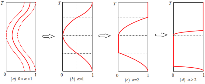
Figure 1. Each rectangle corresponds to the region $[0,1]\times[0,T]$ in $x$-$t$ plane. The limit of $\lambda(D)$ as $D\to 0$ is determined by the average of $V$ over the red solid curves, illustrated for various ranges of $\alpha$ and $m(x,t)=-\frac{\alpha\pi x}{T}\sin\left(\frac{2\pi t}{T}\right)$.

As the proofs of Theorems 1.2, 1.3, and 1.4 are fairly technical, in the following we briefly outline the main strategies in proving Theorems 1.2 and 1.3:

• We note that $\lambda(D)$ for (1.3) in the elliptic situation can be characterized by variational formulation [5, 6, 21, 23]. In contrast, the time-periodic parabolic problem (1.1) has no variational formulations. Our general strategy is to construct super/sub-solutions and apply generalized comparison principle developed in [18, Theorem A.1]. This technique was first introduced by Berestycki and Lions [2] to the elliptic scenario, whereas its adaptation to our context is more subtle because of the presence of temporal variable; see [22] for further discussions.

• We first establish Theorem 1.3 which assumes that $\partial_{x}m$ is strictly positive, negative, or identically zero in each sub-interval $(\kappa_{i},\kappa_{i+1})$. The main difficulty is to establish the lower bound of the principal eigenvalue in (1.5). The construction of super-solutions near the curves $\{(\kappa_{i},t),t\in[0,T]\}$ is rather subtle, due to the fact that the spatio-temporal derivatives of the principal eigenfunction of (1.1) restricted to the curves may be unbounded as $D$ tends to zero. Our strategy is to construct the super-solution almost coinciding with the principal eigenfunction of (1.1) near these curves, and then use an iterated argument to extend the super-solution to the whole domain.

• A key ingredient in the proof of Theorem 1.2 is to recognize the critical role of the solutions of (1.4). Our idea is to reduce the proof of Theorem 1.2 to that of Theorem 1.3 with $\mathbf{B}=\emptyset$. As Theorem 1.3 assumes that $\partial_{x}m$ is either strictly positive or negative in each sub-interval $(\kappa_{i},\kappa_{i+1})$, there are two difficulty in doing so: First, the solutions $P_{i}(t)$ of (1.4) are not constant ones as specified in Theorem 1.3. This difficulty can be overcome by introducing a proper transformation so that $P_{i}(t)$ become constant after the transformation. The second difficulty is that a priori we do not know the sign of the term $\partial_{x}m$ in each $(\kappa_{i},\kappa_{i+1})$. Our idea is to introduce another transformation, which is associated with the trajectories of (1.4). We prove that after the second transformation, $\partial_{x}m$ is indeed either strictly positive or negative in each $(\kappa_{i},\kappa_{i+1})$, so that the proof of Theorem 1.3 is directly applicable to complete the proof of Theorem 1.2.

This paper is organized as follows: In Section 2 we present some results associated with the case when all of periodic solutions of (1.4) are constants and establish Theorem 1.3. These results are used in Section 3 to give the proof of Theorem 1.2, by combining with an idea of “straightening periodic solutions”. Section 4 is devoted to the proof of Theorem 1.4. A generalized comparison result will be presented in the Appendix.

2. Proof of Theorem 1.3

This section is devoted to the proof of Theorem 1.3. Hereafter, we use $\mathcal{L}_{D}$ to denote the time-periodic parabolic operator

$$\mathcal{L}_{D}:=\partial_{t}-D\partial_{xx}-\partial_{x}m\partial_{x}+V.$$

For any $x\in[0,1]$, we define a $T$-periodic function $f_{x}:[0,T]\to(0,\infty)$ by

(2.1) $$f_{x}(t)=\mbox{exp}\left[-\int_{0}^{t}V(x,s)\mathrm{d}s+\hat{V}(x)t\right],$$

which solves, for fixed $x\in[0,1]$, that $(\log f_{x})^{\prime}=\hat{V}(x)-V(x,t)$.

Proposition 2.1.

For any constant $\kappa\in(0,1)$, suppose that

$$\begin{cases}\partial_{x}m(x,t)>0,&(x,t)\in[0,\kappa)\times[0,T],\\ \partial_{x}m(x,t)<0,&(x,t)\in(\kappa,1]\times[0,T].\\ \end{cases}$$

Then we have

$$\lim_{D\rightarrow 0}\lambda(D)=\hat{V}(\kappa).$$

Proof.

We first prove the upper bound

(2.2) $$\limsup_{D\to 0}\lambda(D)\leq\hat{V}(\kappa).$$

Fix any $\epsilon>0$. For sufficiently small $D$, we construct a strict non-negative sub-solution $\underline{\varphi}$ in the sense of Definition A.1 (see Appendix A) such that

(2.3) $$\begin{cases}\vskip 3.0pt plus 1.0pt minus 1.0pt\mathcal{L}_{D}\underline{\varphi}\leq\left[\hat{V}(\kappa)+\epsilon\right]\underline{\varphi}&\text{in}\,\,((0,1)\setminus\mathbb{X})\times(0,T),\\ \vskip 6.0pt plus 2.0pt minus 2.0pt\partial_{x}\underline{\varphi}(0,t)=\partial_{x}\underline{\varphi}(1,t)=0&\text{on}\,\,[0,T],\\ \underline{\varphi}(x,0)=\underline{\varphi}(x,T)&\text{on}\,\,(0,1),\end{cases}$$

for some point set $\mathbb{X}$ determined later.

To this end, by continuity of $V$, we choose small $\delta\in(0,1)$ such that

(2.4) $$|V(x,t)-V(\kappa,t)|<\epsilon/2\quad\text{on}\quad[\kappa-\delta,\kappa+\delta]\times[0,T].$$

Then we define $\underline{\varphi}$ by

$$\underline{\varphi}(x,t):=f_{\kappa}(t)\cdot\underline{z}(x),$$

where $f_{\kappa}(t)$ is defined in (2.1) with $x=\kappa$, and $\underline{z}\in C([0,1])$ is given by

(2.5) $$\underline{z}(x):=\begin{cases}\vskip 3.0pt plus 1.0pt minus 1.0pt-(x-\kappa)^{2}+\delta^{2}&\text{ on }[\kappa-\delta,\kappa+\delta],\\ 0&\text{ on }[0,\kappa-\delta)\cup(\kappa+\delta,1].\end{cases}$$

Observe that $\partial_{x}\underline{\varphi}\left(\left(\kappa\pm\delta\right)^{+},\cdot\right)>\partial_{x}\underline{\varphi}\left(\left(\kappa\pm\delta\right)^{-},\cdot\right)$. We now identify $\mathbb{X}$ in (2.3) as

$$\begin{array}[]{c}\mathbb{X}=\{\kappa\pm\delta\}.\end{array}$$

To verify (2.3), note from definition (2.1) that $f^{\prime}_{\kappa}=(\hat{V}(\kappa)-V(\kappa,t))f_{\kappa}$, direct calculations on $[\kappa-\delta,\kappa+\delta]\times[0,T]$ yield that for small $D$,

$$\begin{split}\mathcal{L}_{D}\underline{\varphi}&=f^{\prime}_{\kappa}(t)\underline{z}-D\partial_{xx}\underline{\varphi}-\partial_{x}m\partial_{x}\underline{\varphi}+V(x,t)\underline{\varphi}\\ &=\left[\hat{V}(\kappa)-V\left(\kappa,t\right)+V(x,t)\right]\underline{\varphi}-\partial_{x}m\partial_{x}\underline{\varphi}-D\partial_{xx}\underline{\varphi}\\ &\leq\left[\hat{V}(\kappa)+\epsilon/2\right]\underline{\varphi}-\partial_{x}m\partial_{x}\underline{\varphi}-D\partial_{xx}\underline{\varphi}\\ &\leq\left[\hat{V}(\kappa)+\epsilon\right]\underline{\varphi},\end{split}$$

where $-\partial_{x}m\partial_{x}\underline{\varphi}-D\partial_{xx}\underline{\varphi}\leq\frac{\epsilon}{2}\underline{\varphi}$ in the last inequality is due to the fact that $-\partial_{x}m\partial_{x}\underline{\varphi}<0\leq\epsilon\underline{\varphi}$ in the neighborhoods of $\{\kappa\pm\delta\}\times[0,T]$. Hence (2.3) holds, and (2.2) follows from (2.3) and Proposition A.1 by letting $\epsilon\to 0^{+}$.

Next, we show that

(2.6) $$\liminf_{D\to 0}\lambda(D)\geq\hat{V}(\kappa).$$

Define $\overline{\varphi}\in C^{2,1}([0,1]\times[0,T])$ by

$$\overline{\varphi}(x,t):=f_{\kappa}(t)\cdot e^{M_{1}(x-\kappa)^{2}}$$

with $M_{1}>0$ to be specified later. For any given $\epsilon>0$, we shall choose $M_{1}$ large so that for sufficiently small $D$, $\overline{\varphi}$ satisfies

(2.7) $$\begin{cases}\vskip 3.0pt plus 1.0pt minus 1.0pt\mathcal{L}_{D}\overline{\varphi}\geq\left[\hat{V}(\kappa)-\epsilon\right]\overline{\varphi}&\text{in}\,\,(0,1)\times(0,T),\\ \vskip 3.0pt plus 1.0pt minus 1.0pt\partial_{x}\overline{\varphi}(0,t)<0<\partial_{x}\overline{\varphi}(1,t)&\text{on}\,\,[0,T],\\ \overline{\varphi}(x,0)=\overline{\varphi}(x,T)&\text{on}\,\,(0,1).\end{cases}$$

To establish (2.7), we first recall that $\delta$ is chosen as in (2.4). For $x\in(0,\kappa-\delta]\cup[\kappa+\delta,1)$, there exists some $\epsilon_{0}>0$ such that $|\partial_{x}m|\geq\epsilon_{0}$, and thus

$$-\partial_{x}m\partial_{x}(\log\overline{\varphi})=2M_{1}\partial_{x}m\cdot(x-\kappa)\geq 2M_{1}\delta\epsilon_{0},$$

from which direct calculation leads to

(2.8) $$\begin{split}\mathcal{L}_{D}\overline{\varphi}&\geq\left\{\hat{V}(\kappa)+V(x,t)-V\left(\kappa,t\right)-D\left[2M_{1}+4M_{1}^{2}(x-\kappa)^{2}\right]+2M_{1}\delta\epsilon_{0}\right\}\overline{\varphi}.\end{split}$$

We choose $M_{1}$ large such that $2M_{1}\delta\epsilon_{0}>2\|V\|_{L^{\infty}}$. Letting $D$ be small enough in (2.8), we deduce $\mathcal{L}_{D}\overline{\varphi}\geq\hat{V}(\kappa)\overline{\varphi}$ as desired.

For $x\in[\kappa-\delta,\kappa+\delta]$, by $-\partial_{x}m\partial_{x}\overline{\varphi}\geq 0$ and the definition of $\delta$ we have

$$\begin{split}\mathcal{L}_{D}\overline{\varphi}\geq\left\{\hat{V}(\kappa)+V(x,t)-V\left(\kappa,t\right)-D\left[2M_{1}+4M_{1}^{2}(x-\kappa)^{2}\right]\right\}\overline{\varphi}\geq\left[\hat{V}(\kappa)-\epsilon\right]\overline{\varphi}\end{split}$$

for sufficiently small $D$.

Therefore, (2.7) holds and (2.6) follows from Proposition A.1 with $\mathbb{X}=\emptyset$. ∎

To proceed further, we will need the following result:

Lemma 2.2.

Let $\rho(t)\geq 0\,(\not\equiv 0)$ be any $T$-periodic function. For each $R>0$, denote by $\mu_{R}$ the principal eigenvalue of the following problem:

(2.9) $$\begin{cases}\vskip 3.0pt plus 1.0pt minus 1.0pt\partial_{t}\varphi-\partial_{xx}\varphi-x\rho(t)\partial_{x}\varphi=\mu_{R}\varphi&\text{in}\,\,(-R,R)\times(0,T),\\ \vskip 3.0pt plus 1.0pt minus 1.0pt\varphi(-R,t)=\varphi(R,t)=0&\text{on}\,\,[0,T],\\ \varphi(x,0)=\varphi(x,T)&\text{on}\,\,[-R,R].\end{cases}$$

Then we have

$$\lim_{R\to\infty}\mu_{R}=\hat{\rho}.$$

Proof.

For each $\delta\geq 0$, in view of $\rho(t)\geq 0\,(\not\equiv 0)$ in $[0,T]$, we choose $\beta_{\delta}(t)$ as the unique positive solution of the problem

(2.10) $$\begin{cases}\vskip 3.0pt plus 1.0pt minus 1.0pt\frac{\dot{\beta}(t)}{2}=\beta(t)\left[\rho(t)+\delta-\beta(t)\right]\,\,\text{ in }\,[0,T],\\ \beta(0)=\beta(T).\end{cases}$$

Denote by $(\alpha_{\delta}(t),\mu_{\delta})$ an eigenpair, with $\alpha_{\delta}(t)>0$, of the eigenvalue problem

(2.11) $$\begin{cases}\vskip 3.0pt plus 1.0pt minus 1.0pt\dot{\alpha}(t)+\beta_{\delta}(t)\alpha(t)=\mu\alpha(t)\,\,\text{ in }[0,T],\\ \alpha(0)=\alpha(T).\end{cases}$$

Dividing both sides of (2.10) by $\beta_{\delta}$, and integrating the resulting equation over $[0,T]$, by periodicity of $\beta_{\delta}$ we have $\hat{\beta}_{\delta}=\hat{\rho}+\delta.$ Similarly, (2.11) implies $\mu_{\delta}=\hat{\beta}_{\delta}$. Therefore,

(2.12) $$\mu_{\delta}=\hat{\beta}_{\delta}=\hat{\rho}+\delta.$$

For any $\delta\geq 0$, we define $T$-periodic function $\psi_{\delta}\in C^{2,1}(\mathbb{R}\times[0,T])$ by

(2.13) $$\psi_{\delta}(x,t):=\alpha_{\delta}(t)e^{-\frac{\beta_{\delta}(t)}{2}x^{2}},$$

which, by definitions (2.10) and (2.11), solves

(2.14) $$\mathcal{L}_{\delta}\psi_{\delta}:=\partial_{t}\psi_{\delta}-\partial_{xx}\psi_{\delta}-x(\rho(t)+\delta)\partial_{x}\psi_{\delta}=\mu_{\delta}\psi_{\delta}\quad\text{ in }\quad\mathbb{R}\times[0,T].$$

We first show $\liminf_{R\to\infty}\mu_{R}\geq\hat{\rho}$. For $\delta=0$, $\psi_{0}$ defined by (2.13) is a super-solution to (2.9) in the sense of Definition A.1 for any $R>0$. By Proposition A.1, we have $\mu_{R}\geq\mu_{0}=\hat{\rho}$ for any $R>0$, and thus $\liminf_{R\to\infty}\mu_{R}\geq\hat{\rho}$.

Next, we show $\limsup_{R\to\infty}\mu_{R}\leq\hat{\rho}$. Fix any $\delta>0$. Choose $R_{\delta}>0$ large such that $\delta x^{2}\beta_{\delta}(t)\geq\hat{\rho}+\delta$ for all $|x|\geq R_{\delta}$ and $t\in[0,T]$. Then let $\epsilon=\epsilon(\delta)>0$ be small so that $\delta\psi_{\delta}(R_{\delta},t)\geq\epsilon(\hat{\rho}+2\delta)$ for all $t\in[0,T]$. Set $\tilde{\psi}_{\delta}=\max\{\psi_{\delta}-\epsilon,0\}$. Note that we can choose $\epsilon$ smaller if necessary such that $\tilde{\psi}_{\delta}(x,t)>0$ holds for all $|x|\leq R_{\delta}$ and $t\in[0,T]$.

On $\{(x,t):\tilde{\psi}_{\delta}(x,t)>0,|x|\geq R_{\delta}\}$, by (2.12) and (2.14) we calculate that

(2.15) $$\begin{split}&\partial_{t}\tilde{\psi}_{\delta}-\partial_{xx}\tilde{\psi}_{\delta}-x\rho(t)\partial_{x}\tilde{\psi}_{\delta}-(\hat{\rho}+2\delta)\tilde{\psi}_{\delta}\\ =&(\hat{\rho}+\delta)\psi_{\delta}-\delta x^{2}\beta_{\delta}(t)\psi_{\delta}-(\hat{\rho}+2\delta)(\psi_{\delta}-\epsilon)\\ \leq&(\hat{\rho}+\delta)\psi_{\delta}-\delta x^{2}\beta_{\delta}(t)\psi_{\delta}\\ \leq&0,\end{split}$$

where the last inequality follows from the choice of $R_{\delta}$.

On $\{(x,t):\tilde{\psi}_{\delta}(x,t)>0,|x|\leq R_{\delta}\}$, we have

(2.16) $$\begin{split}&\partial_{t}\tilde{\psi}_{\delta}-\partial_{xx}\tilde{\psi}_{\delta}-x\rho(t)\partial_{x}\tilde{\psi}_{\delta}-(\hat{\rho}+2\delta)\tilde{\psi}_{\delta}\\ =&(\hat{\rho}+\delta)\psi_{\delta}-\delta x^{2}\beta_{\delta}(t)\psi_{\delta}-(\hat{\rho}+2\delta)(\psi_{\delta}-\epsilon)\\ \leq&(\hat{\rho}+\delta)\psi_{\delta}-(\hat{\rho}+2\delta)(\psi_{\delta}-\epsilon)\\ \leq&\epsilon(\hat{\rho}+2\delta)-\delta\psi_{\delta}(R_{\delta},t)\\ \leq&0,\end{split}$$

where the last inequality is due to the choice of $\epsilon$.

Choose some large $\tilde{R}_{\delta}>R_{\delta}$ such that $\tilde{\psi}_{\delta}(\tilde{R}_{\delta},t)=0$ for all $t\in[0,T]$. By (2.15) and (2.16), the constructed $\tilde{\psi}_{\delta}$ is a sub-solution to (2.9) in the sense of Definition A.1 for any $R\geq\tilde{R}_{\delta}$. A direct application of Proposition A.1 yields $\mu_{R}\leq\hat{\rho}+2\delta$ for all $R\geq\tilde{R}_{\delta}$, and thus $\limsup_{R\to\infty}\mu_{R}\leq\hat{\rho}+2\delta$. Letting $\delta\to 0$ completes the proof. ∎

Proposition 2.3.

For any $\kappa\in(0,1)$, suppose that

$$\begin{cases}\partial_{x}m(x,t)<0,&(x,t)\in(0,\kappa)\times[0,T],\\ \partial_{x}m(x,t)>0,&(x,t)\in(\kappa,1)\times[0,T],\\ \partial_{xx}m(\kappa,t)\geq(\not\equiv)0,&t\in[0,T],\\ m(x,0)=m(x,T),&x\in[0,1].\end{cases}$$

Then we have

$$\lim_{D\rightarrow 0}\lambda(D)=\min\left\{\hat{V}(0),\ \hat{V}(\kappa)+\partial_{xx}\hat{m}(\kappa),\ \hat{V}(1)\right\}.$$

Proof.

For any given $\epsilon>0$, we choose some small $\delta>0$ such that

(2.17) $$\begin{array}[]{ll}\vskip 6.0pt plus 2.0pt minus 2.0pt|V(x,t)-V(0,t)|<\epsilon/2,&(x,t)\in[0,\delta]\times[0,T],\\ \vskip 6.0pt plus 2.0pt minus 2.0pt|V(x,t)-V(\kappa,t)|<\epsilon/2,&(x,t)\in\left[\kappa-\delta,\kappa+\delta\right]\times[0,T],\\ |V(x,t)-V(1,t)|<\epsilon/2,&(x,t)\in[1-\delta,1]\times\in[0,T].\end{array}$$

Part I. In this part, we establish the upper bound

$$\limsup_{D\rightarrow 0}\lambda(D)\leq\lambda_{\min}:=\min\left\{\hat{V}(0),\ \hat{V}(\kappa)+\partial_{xx}\hat{m}(\kappa),\ \hat{V}(1)\right\}.$$

By a similar argument as in Proposition 2.1, it is straightforward to show that

$$\limsup_{D\rightarrow 0}\lambda(D)\leq\min\left\{\hat{V}(0),\ \hat{V}(1)\right\}.$$

It remains to prove

(2.18) $$\limsup_{D\rightarrow 0}\lambda(D)\leq\hat{V}(\kappa)+\partial_{xx}\hat{m}(\kappa).$$

Fix any $\epsilon>0$. For sufficiently small $D$, we construct a sub-solution $\underline{\varphi}$ such that

(2.19) $$\begin{cases}\vskip 3.0pt plus 1.0pt minus 1.0pt\mathcal{L}_{D}\underline{\varphi}\leq\left[\hat{V}(\kappa)+\partial_{xx}\hat{m}(\kappa)+2\epsilon\right]\underline{\varphi}&\text{in}\,\,((0,1)\setminus\mathbb{X})\times[0,T],\\ \vskip 3.0pt plus 1.0pt minus 1.0pt\partial_{x}\underline{\varphi}(0,t)=\partial_{x}\underline{\varphi}(1,t)=0&\text{on}\,\,[0,T],\\ \underline{\varphi}(x,0)=\underline{\varphi}(x,T)&\text{on}\,\,(0,1),\end{cases}$$

where the set $\mathbb{X}$ will be determined later.

To this end, we define

$$\bar{m}(x,t):=[\partial_{xx}m(\kappa,t)+\epsilon]\cdot\tfrac{\left(x-\kappa\right)^{2}}{2},$$

and further choose $\delta$ smaller if necessary such that

(2.20) $$\begin{array}[]{c}|\partial_{x}\bar{m}|\geq|\partial_{x}m|~{}\,\,~{}\text{ in }~{}\left[\kappa-\delta,\kappa+\delta\right]\times[0,T].\end{array}$$

Let $\bar{\lambda}_{D}$ denote the principal eigenvalue of the problem

(2.21) $$\begin{cases}\vskip 3.0pt plus 1.0pt minus 1.0pt\partial_{t}\psi-D\partial_{xx}\psi-\partial_{x}\bar{m}\partial_{x}\psi=\bar{\lambda}_{D}\psi&\text{in}\,\,(\kappa-\delta,\kappa+\delta)\times[0,T],\\ \psi(\kappa-\delta,t)=\psi(\kappa+\delta,t)=0&\text{on}\,\,[0,T],\\ \psi(x,0)=\psi(x,T)&\text{on}\,\,[\kappa-\delta,\kappa+\delta],\end{cases}$$

and the corresponding eigenfunction $\underline{\psi}_{D}$ is chosen to be positive in $(\kappa-\delta,\kappa+\delta)\times[0,T]$. Under the scaling $y=\frac{x-\kappa}{\sqrt{D}}$, we set $\underline{\varphi}_{D}(y,t):=\underline{\psi}_{D}(\sqrt{D}y+\kappa,t)$, which is the principal eigenfunction (associated to $\bar{\lambda}_{D}$) of the problem

$$\begin{cases}\vskip 3.0pt plus 1.0pt minus 1.0pt\partial_{t}\varphi-\partial_{yy}\varphi-y[\partial_{xx}m(\kappa,t)+\epsilon]\partial_{y}\varphi=\bar{\lambda}_{D}\varphi&\text{in}\,\,\left(-\frac{\delta}{\sqrt{D}},\frac{\delta}{\sqrt{D}}\right)\times[0,T],\\ \vskip 3.0pt plus 1.0pt minus 1.0pt\varphi(-\frac{\delta}{\sqrt{D}},t)=\varphi(\frac{\delta}{\sqrt{D}},t)=0&\text{on}\,\,[0,T],\\ \varphi(x,0)=\varphi(x,T)&\text{on}\,\,\left[-\frac{\delta}{\sqrt{D}},\frac{\delta}{\sqrt{D}}\right].\end{cases}$$

By Lemma 2.2, we deduce that

(2.22) $$\lim_{D\to 0}\bar{\lambda}_{D}=\partial_{xx}\hat{m}(\kappa)+\epsilon.$$

We extend $\underline{\psi}_{D}$, the principal eigenfunction of (2.21), to $[0,1]\times[0,T]$ by setting

$$\underline{\psi}_{D}\equiv 0\quad\text{on}\quad([0,\kappa-\delta]\cup[\kappa+\delta,1])\times[0,T].$$

Applying the Hopf boundary lemma to (2.21), we have

$$\partial_{x}\underline{\psi}_{D}\left((\kappa-\delta)^{+},\cdot\right)>0=\partial_{x}\underline{\psi}_{D}\left((\kappa-\delta)^{-},\cdot\right),$$

$$\partial_{x}\underline{\psi}_{D}\left((\kappa+\delta)^{+},\cdot\right)=0>\partial_{x}\underline{\psi}_{D}\left((\kappa+\delta)^{-},\cdot\right),$$

so that we choose $\mathbb{X}$ by $\mathbb{X}=\{\kappa\pm\delta\}$.

Define

$$\underline{\varphi}(x,t)=f_{\kappa}(t)\cdot\underline{\psi}_{D}(x,t)\quad\text{in}\quad[0,1]\times[0,T],$$

where $f_{\kappa}(t)$ is given by (2.1) with $x=\kappa$. We verify that $\underline{\varphi}$ satisfies (2.19). By properties of $\underline{\psi}_{D}$ and (2.20) we can derive that

$$-\partial_{x}m\partial_{x}\underline{\psi}_{D}\leq-\partial_{x}\bar{m}\partial_{x}\underline{\psi}_{D}\quad\text{ in }\quad[0,1]\times[0,T].$$

Hence, direct calculations on $((0,1)\setminus\mathbb{X})\times[0,T]$ give

$$\begin{split}\mathcal{L}_{D}\underline{\varphi}=&\left[-V\left(\kappa,t\right)+\hat{V}\left(\kappa\right)+V(x,t)\right]\underline{\varphi}+\left[\partial_{t}\underline{\psi}_{D}-D\partial_{xx}\underline{\psi}_{D}-\partial_{x}m\partial_{x}\underline{\psi}_{D}\right]f_{\kappa}(t)\\ \leq&\left[\hat{V}\left(\kappa\right)+\epsilon/2\right]\underline{\varphi}+\left[\partial_{t}\underline{\psi}_{D}-D\partial_{xx}\underline{\psi}_{D}-\partial_{x}\bar{m}\partial_{x}\underline{\psi}_{D}\right]f_{\kappa}(t)\\ =&\left[\hat{V}\left(\kappa\right)+\bar{\lambda}_{D}+\epsilon/2\right]\underline{\varphi}\\ \leq&\left[\hat{V}\left(\kappa\right)+\partial_{xx}\hat{m}(\kappa)+2\epsilon\right]\underline{\varphi},\end{split}$$

provided that $D$ is small enough, where the last inequality is a consequence of (2.22). Therefore, $\underline{\varphi}$ defines a sub-solution satisfying (2.19), which together with Proposition A.1 implies (2.18).

Part II. We shall establish the lower bound

(2.23) $$\liminf_{D\rightarrow 0}\lambda(D)\geq\lambda_{\min}:=\min\left\{\hat{V}(0),\ \hat{V}(\kappa)+\partial_{xx}\hat{m}(\kappa),\ \hat{V}(1)\right\}.$$

For each small $\epsilon>0$, the main ingredient in the proof is to construct a positive continuous super-solution $\overline{\varphi}$ in the sense of Definition A.1, i.e. for sufficiently small $D$,

(2.24) $$\begin{cases}\vskip 3.0pt plus 1.0pt minus 1.0pt\mathcal{L}_{D}\overline{\varphi}\geq(1-\epsilon)(\lambda_{\min}-\epsilon)\overline{\varphi}&\text{in}\,\,((0,1)\setminus\mathbb{X})\times[0,T],\\ \vskip 3.0pt plus 1.0pt minus 1.0pt\partial_{x}\overline{\varphi}(0,t)=\partial_{x}\overline{\varphi}(1,t)=0&\text{on}\,\,[0,T],\\ \overline{\varphi}(x,0)=\overline{\varphi}(x,T)&\text{on}\,\,(0,1),\end{cases}$$

where the point set $\mathbb{X}$ will be determined in Step 3. Then (2.23) follows from Proposition A.1 and arbitrariness of $\epsilon$.

Step 1. We prepare some notations. First, we choose suitable $T$-periodic function $\underline{\rho}(t)\geq\not\equiv 0$ and small $\delta>0$ such that

(2.25) $$\begin{cases}\vskip 3.0pt plus 1.0pt minus 1.0pt\max\{\partial_{xx}m(\kappa,t)-\epsilon,0\}\leq\underline{\rho}(t)\leq\partial_{xx}m(\kappa,t),\quad t\in[0,T],\\ \underline{\rho}(t)|x-\kappa|\leq|\partial_{x}m(x,t)|,\quad(x,t)\in[\kappa-\delta,\kappa+\delta]\times[0,T].\end{cases}$$

Due to $\hat{\underline{\rho}}>0$, define $r(t)$ as the unique positive $T$-periodic solution of

(2.26) $$\frac{\dot{r}(t)}{2-\ell}=r(t)\left[\underline{\rho}(t)-\left(\frac{4}{(2-\ell)^{2}}+\frac{\epsilon}{2}\right)r(t)\right],$$

where the small parameter $\ell\in(0,\epsilon/2]$ can be specified as follows: Note that there exist $0<\underline{r}<\overline{r}$ independent of $\ell\in(0,\epsilon/2]$ such that

$$0<\underline{r}<r(t)<\overline{r}\quad\text{ for all }t\in[0,T]\text{ and }\ell\in[0,\epsilon/2].$$

We fix $\ell\in(0,\epsilon/2]$ small such that

(2.27) $$\begin{cases}\vskip 3.0pt plus 1.0pt minus 1.0pt\frac{\frac{2}{2-\ell}}{\frac{4}{(2-\ell)^{2}}+\frac{\epsilon}{2}}\geq 1-\epsilon,\\ \nu:=\frac{\ell\overline{r}}{2-\ell}<\left[\sqrt{\frac{4}{(2-\ell)^{2}}+\frac{\epsilon}{2}}-1\right]\underline{r}.\end{cases}$$

Without loss of generality, we assume there is some $n_{*}\in\mathbb{N}$ ($n_{*}>3$) such that

(2.28) $$1/\ell=2^{n_{*}-2},$$

and further choose $\delta$ smaller if necessary such that

$$\delta<\kappa-(n_{*}+1)\delta<\kappa+(n_{*}+1)\delta<1-\delta.$$

For fixed $r(t)$ and $\ell$, we define $(\alpha_{1}(t),\lambda_{\ell})$ as the eigenpair of

(2.29) $$\begin{cases}\vskip 3.0pt plus 1.0pt minus 1.0pt\dot{\alpha}_{1}(t)+\frac{2}{2-\ell}\alpha_{1}(t)r(t)=\lambda_{\ell}\alpha_{1}(t)&\text{ in }[0,T],\\ \alpha_{1}(0)=\alpha_{1}(T).\end{cases}$$

Similar to (2.12), we deduce from (2.26) and (2.29) that

$$\lambda_{\ell}=\frac{2}{2-\ell}\hat{r}=\frac{\frac{2}{2-\ell}}{\frac{4}{(2-\ell)^{2}}+\frac{\epsilon}{2}}\hat{\underline{\rho}},$$

which, together with (2.27), leads to

(2.30) $$\lambda_{\ell}\geq(1-\epsilon)\hat{\underline{\rho}}.$$

Step 2. We construct a positive super-solution $\overline{\psi}\in C(\mathbb{R}\times[0,T])$ for the auxiliary problem

(2.31) $$\begin{cases}\vskip 3.0pt plus 1.0pt minus 1.0pt\partial_{t}\psi-\partial_{yy}\psi-y\underline{\rho}(t)\partial_{y}\psi=(1-\epsilon)\hat{\underline{\rho}}\psi&\text{in}\,\,\mathbb{R}\times[0,T],\\ \psi(x,0)=\psi(x,T)&\text{on}\,\,\mathbb{R}.\end{cases}$$

Using the notations introduced in Step 1, we define

(2.32) $$\overline{\psi}(y,t):=\begin{cases}\vskip 3.0pt plus 1.0pt minus 1.0pt\alpha_{1}(t)e^{-\frac{r(t)}{2-\ell}y^{2}}&\mbox{ on }[-y_{0},y_{0}]\times[0,T],\\ \vskip 3.0pt plus 1.0pt minus 1.0pt\eta_{1}(t)e^{-\frac{(r(t)+\nu)y_{0}^{\ell}}{2-\ell}y^{2-\ell}}&\mbox{ on }(y_{0},\infty)\times[0,T],\\ \eta_{1}(t)e^{-\frac{(r(t)+\nu)y_{0}^{\ell}}{2-\ell}(-y)^{2-\ell}}&\mbox{ on }(-\infty,-y_{0})\times[0,T],\\ \end{cases}$$

where $y_{0}$ is a constant to be determined later, and $\eta_{1}(t)=\alpha_{1}(t)e^{\frac{\nu y_{0}^{2}}{2-\ell}}$, so that $\overline{\psi}\in C(\mathbb{R}\times[0,T])$ and $(\log\eta_{1})^{\prime}=(\log\alpha_{1})^{\prime}$ independent of $y_{0}$.

By the definition of $\nu$ in (2.27), we may assert that for any $y_{0}>0$,

(2.33) $$\partial_{y}(\log\overline{\psi})(y_{0}^{-},\cdot)=\left[-\frac{2r(\cdot)}{2-\ell}\right]y_{0}>\left[-(r(\cdot)+\nu)\right]y_{0}=\partial_{y}(\log\overline{\psi})(y_{0}^{+},\cdot),$$

and similarly, $\partial_{y}\overline{\psi}((-y_{0})^{-},\cdot)>\partial_{y}\overline{\psi}((-y_{0})^{+},\cdot)$. Therefore, in view of (2.30), to verify that $\overline{\psi}$ defined by (2.32) is a super-solution of (2.31), it remains to choose large $y_{0}$ such that

(2.34) $$\partial_{t}\overline{\psi}-\partial_{yy}\overline{\psi}-y\underline{\rho}(t)\partial_{y}\overline{\psi}\geq\lambda_{\ell}\overline{\psi}\quad\text{in }\,\,(\mathbb{R}\setminus\{\pm y_{0}\})\times[0,T],$$

which can be verified by the following computations:

• For $y\in(-y_{0},y_{0})$, by (2.26) and (2.32), direct calculations yield

  $$\begin{split}&\partial_{t}\overline{\psi}-\partial_{yy}\overline{\psi}-y\underline{\rho}(t)\partial_{y}\overline{\psi}\\ =&\left[(\log\alpha_{1})^{\prime}-\frac{\dot{r}(t)}{2-\ell}y^{2}+\frac{2r(t)}{2-\ell}-\frac{4r^{2}(t)}{(2-\ell)^{2}}y^{2}+\frac{2r(t)\underline{\rho}(t)}{2-\ell}y^{2}\right]\overline{\psi}\\ \geq&\left[(\log\alpha_{1})^{\prime}+\frac{2r(t)}{2-\ell}\right]\overline{\psi}+\left[-\frac{\dot{r}(t)}{2-\ell}-\frac{4r^{2}(t)}{(2-\ell)^{2}}+r(t)\underline{\rho}(t)\right]y^{2}\overline{\psi}\\ \geq&\left[(\log\alpha_{1})^{\prime}+\frac{2r(t)}{2-\ell}\right]\overline{\psi}\\ =&\lambda_{\ell}\overline{\psi};\end{split}$$

• For $y\in(y_{0},\infty)$, again by (2.26) and (2.32), we calculate that

  $$\begin{split}&\partial_{t}\overline{\psi}-\partial_{yy}\overline{\psi}-y\underline{\rho}(t)\partial_{y}\overline{\psi}-\lambda_{\ell}\overline{\psi}\\ =&\left[(\log\eta_{1})^{\prime}-\lambda_{\ell}\right]\overline{\psi}+y_{0}^{\ell}y^{2-\ell}\left[-\frac{\dot{r}(t)}{2-\ell}+(1-\ell)(r(t)+\nu)y^{-2}\right]\overline{\psi}\\ &+y_{0}^{\ell}y^{2-\ell}\left[-(r(t)+\nu)^{2}y_{0}^{\ell}y^{-\ell}+(r(t)+\nu)\underline{\rho}(t)\right]\overline{\psi}\\ \geq&\left[(\log\alpha_{1})^{\prime}-\lambda_{\ell}\right]\overline{\psi}+y_{0}^{\ell}y^{2-\ell}\left[-\frac{\dot{r}(t)}{2-\ell}-(r(t)+\nu)^{2}+r(t)\underline{\rho}(t)\right]\overline{\psi}\\ =&\left[(\log\alpha_{1})^{\prime}-\lambda_{\ell}\right]\overline{\psi}+y_{0}^{\ell}y^{2-\ell}\left[\left(\frac{4}{(2-\ell)^{2}}+\frac{\epsilon}{2}\right)r^{2}(t)-(r(t)+\nu)^{2}\right]\overline{\psi}.\end{split}$$

  In light of $\left(\frac{4}{(2-\ell)^{2}}+\frac{\epsilon}{2}\right)r^{2}(t)>(r(t)+\nu)^{2}$ (due to (2.27)), we may pick $y_{0}$ large enough to ensure (2.34) on $(y_{0},\infty)\times[0,T]$;

• For $y\in(-\infty,-y_{0})$, we can verify (2.34) by the same argument as in (ii).

Consequently, (2.34) holds true, and $\overline{\psi}$ constructed by (2.32) is a super-solution of (2.31) in the sense of Definition A.1.

In what follows, we divide the construction of super-solution $\overline{\varphi}$ which satisfies (2.24) into the following several steps via separating different regions; see Fig.2 for the profile of $\overline{\varphi}$ to be constructed.

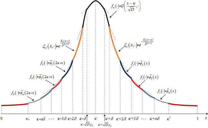
Figure 2. The profile of $\overline{\varphi}$ for fixed $t\in[0,T]$.

Step 3. We construct super-solution $\overline{\varphi}$ on $[\kappa-\delta,\kappa+\delta]\times[0,T]$ satisfying (2.24). Let $\overline{\psi}$ be given by (2.32) with fixed $y_{0}$ chosen in Step 2. We assume $\sqrt{D}y_{0}<\delta$, and define $\mathbb{X}$ by

(2.35) $$\mathbb{X}=\bigcup\limits_{n=1}^{n_{*}}\{\kappa\pm n\delta\}\cup\{\delta,1-\delta\}\cup\left\{\kappa\pm\sqrt{D}y_{0}\right\}.$$

where $n_{*}$ is chosen in (2.28). Set

(2.36) $$\overline{\varphi}(x,t):=f_{\kappa}(t)\cdot\overline{\psi}\left(\frac{x-\kappa}{\sqrt{D}},t\right)\quad\text{on}\quad[\kappa-\delta,\kappa+\delta]\times[0,T],$$

where $f_{\kappa}(t)$ is defined by (2.1) with $x=\kappa$. Note that $\overline{\varphi}$ is symmetric in $x$ with respect to $x=\kappa$, and is decreasing in $x$ for $x\geq\kappa$ and $t\in[0,T]$. Thus by (2.25) and (2.36) we arrive at

(2.37) $$-\partial_{x}m\partial_{x}\overline{\varphi}=|\partial_{x}m|\cdot|\partial_{x}\overline{\varphi}|\geq f_{\kappa}(t)\underline{\rho}(t)\frac{|x-\kappa|}{\sqrt{D}}\left|\partial_{y}\overline{\psi}\left(\frac{x-\kappa}{\sqrt{D}},t\right)\right|=-f_{\kappa}(t)\underline{\rho}(t)\cdot y\partial_{y}\overline{\psi}\left(y,t\right),$$

where $y=\frac{x-\kappa}{\sqrt{D}}$. This implies that on $([\kappa-\delta,\kappa+\delta]\setminus\{\kappa\pm\sqrt{D}y_{0}\})\times[0,T]$,

$$\begin{split}\mathcal{L}_{D}\overline{\varphi}\geq&\left[-V\left(\kappa,t\right)+\hat{V}\left(\kappa\right)+V(x,t)\right]\overline{\varphi}+\left[\partial_{t}\overline{\psi}-\partial_{yy}\overline{\psi}-\underline{\rho}(t)y\partial_{y}\overline{\psi}\right]f_{\kappa}(t)\\ \geq&\left[\hat{V}\left(\kappa\right)-\epsilon/2+(1-\epsilon)\hat{\underline{\rho}}\right]\overline{\varphi}\\ \geq&\left[\hat{V}(\kappa)+(1-\epsilon)\partial_{xx}\hat{m}(\kappa)-\epsilon(1-\epsilon)\right]\overline{\varphi}\\ \geq&(1-\epsilon)(\lambda_{\min}-\epsilon)\overline{\varphi},\end{split}$$

where the first inequality is due to (2.37), the second inequality follows from (2.17) and the fact that $\overline{\psi}$ is a super-solution of (2.31) (see Step 2), and the third inequality follows from (2.25).

On the other hand, by (2.33), we have

$$\partial_{x}(\log\overline{\varphi})((\kappa+\sqrt{D}y_{0})^{+},\cdot)<\partial_{x}(\log\overline{\varphi})((\kappa+\sqrt{D}y_{0})^{-},\cdot)\quad\quad(\text{as}\quad\kappa+\sqrt{D}y_{0}\in\mathbb{X}).$$

Therefore, $\overline{\varphi}$ defined by (2.36) satisfies (2.24) on $[\kappa-\delta,\kappa+\delta]\times[0,T]$.

Step 4. We construct $\overline{\varphi}$ which satisfies (2.24) on $(\kappa+\delta,\kappa+2\delta]\times[0,T]$. Since $\sqrt{D}y_{0}<\delta$, by (2.36) in Step 3 and (2.32) in Step 2, we have

(2.38) $$\begin{cases}\vskip 3.0pt plus 1.0pt minus 1.0pt\log\overline{\varphi}(\kappa+\delta,t)=\log f_{\kappa}(t)+\log\eta_{1}(t)-\frac{(r(t)+\nu)y_{0}^{\ell}\delta^{2-\ell}}{(2-\ell)D^{1-\ell/2}},\\ \partial_{x}(\log\overline{\varphi})((\kappa+\delta)^{-},\cdot)=-(r(\cdot)+\nu)\frac{y_{0}^{\ell}\delta^{1-\ell}}{D^{1-\ell/2}},\end{cases}$$

whence there is some constant $K_{0}>0$ such that

(2.39) $$\left|\partial_{t}(\log\overline{\varphi})(\kappa+\delta,\cdot)\right|=\left|(\log f_{\kappa})^{\prime}+(\log\eta_{1})^{\prime}-\frac{\dot{r}(t)y_{0}^{\ell}\delta^{2-\ell}}{(2-\ell)D^{1-\ell/2}}\right|<\frac{K_{0}}{D^{1-\ell/2}}.$$

We introduce a small parameter $\epsilon_{0}>0$ such that

$$|\partial_{x}m|\geq\epsilon_{0}\quad\text{on}\quad([\delta,\kappa-\delta]\cup[\kappa+\delta,1-\delta])\times[0,T],$$

and fix constant $K_{1}$ so that

$$K_{1}>(\bar{r}+\nu)y_{0}^{\ell}\delta^{1-\ell}+2K_{0}/\epsilon_{0}.$$

Then we define

(2.40) $$\overline{\varphi}(x,t):=\zeta_{1}(x,t)\cdot e^{-\frac{K_{1}(x-\kappa)}{D^{1-\ell/2}}}\quad\text{ on }\,\,(\kappa+\delta,\kappa+2\delta]\times[0,T].$$

Here $\zeta_{1}\in C^{2,1}((\kappa+\delta,\kappa+2\delta)\times[0,T])$ is determined by

(2.41) $$\begin{array}[]{l}\log\zeta_{1}(x,t)=\left[\frac{(\kappa+2\delta)-x}{\delta}\right]\cdot\left[\frac{K_{1}\delta}{D^{1-\ell/2}}+\log\overline{\varphi}(\kappa+\delta,t)\right]+\left[\frac{x-(\kappa+\delta)}{\delta}\right]\log f_{1}(t),\end{array}$$

with $T$-periodic function $f_{1}(t)$ defined in (2.1) with $x=1$, so that

$$\zeta_{1}(\kappa+\delta,t)=e^{\frac{K_{1}\delta}{D^{1-\ell/2}}}\cdot\overline{\varphi}(\kappa+\delta,t).$$

This implies immediately that $\overline{\varphi}$ defined by (2.40) is continuous at $\{\kappa+\delta\}\times[0,T]$. In light of $\partial_{x}\zeta_{1}<0$ (for small $D$), using (2.38) and (2.40), by choice of $K_{1}$ we can verify that

$$\partial_{x}(\log\overline{\varphi})((\kappa+\delta)^{+},\cdot)<-K_{1}/D^{1-\ell/2}<\partial_{x}(\log\overline{\varphi})((\kappa+\delta)^{-},\cdot)\quad\quad(\text{as}\quad\kappa+\delta\in\mathbb{X}).$$

On the other hand, combined with (2.38), (2.39), and (2.41), it is easily seen that

$$\left|\partial_{t}(\log\zeta_{1})\right|<\frac{2K_{0}}{D^{1-\ell/2}},\quad-\frac{3K_{1}}{D^{1-\ell/2}}<\partial_{x}(\log\zeta_{1})<0,\quad\text{and}\quad\partial_{xx}(\log\zeta_{1})=0$$

for small $D$, and thus

$$\left|\frac{\partial_{xx}\zeta_{1}}{\zeta_{1}}\right|=\left|\partial_{xx}(\log\zeta_{1})+[\partial_{x}(\log\zeta_{1})]^{2}\right|<\frac{9K_{1}^{2}}{D^{2-\ell}},$$

from which, using (2.40) and $-\partial_{x}m\cdot\partial_{x}(\log\zeta_{1})\geq 0$, we may calculate that

$$\begin{split}\mathcal{L}_{D}\overline{\varphi}=&\left\{\partial_{t}(\log\zeta_{1})-D\left[\frac{\partial_{xx}\zeta_{1}}{\zeta_{1}}-\frac{2K_{1}}{D^{1-\ell/2}}\partial_{x}(\log\zeta_{1})+\frac{K_{1}^{2}}{D^{2-\ell}}\right]\right\}\overline{\varphi}\\ &+\left\{-\partial_{x}m\cdot\left[\partial_{x}(\log\zeta_{1})-\frac{K_{1}}{D^{1-\ell/2}}\right]+V\right\}\overline{\varphi}\\ \geq&\left[-\frac{2K_{0}}{D^{1-\ell/2}}-\frac{16K_{1}^{2}}{D^{1-\ell}}+\frac{\epsilon_{0}K_{1}}{D^{1-\ell/2}}+V\right]\overline{\varphi}\\ =&\frac{1}{D^{1-\ell/2}}\left[-2K_{0}+\epsilon_{0}K_{1}-16K_{1}^{2}D^{\ell/2}+D^{1-\ell/2}V\right]\overline{\varphi}.\end{split}$$

Since $\epsilon_{0}K_{1}>2K_{0}$ (by the definition of $K_{1}$), we may choose $D$ small such that (2.24) holds. Step 4 is thereby completed.

Step 5. We construct $\overline{\varphi}$ on $(\kappa+2\delta,\kappa+3\delta]\times[0,T]$. By (2.40) and (2.41) in Step 4, we have

(2.42) $$\log\overline{\varphi}(\kappa+2\delta,t)=\log f_{1}(t)-\frac{2K_{1}\delta}{D^{1-\ell/2}}\quad\text{and}\quad\partial_{x}(\log\overline{\varphi})((\kappa+2\delta)^{-},\cdot)>-\frac{4K_{1}}{D^{1-\ell/2}}.$$

Fix a constant $K_{2}$ such that $K_{2}>16K_{1}^{2}/\epsilon_{0}$, where $\epsilon_{0}$ is given in Step 4 such that $\partial_{x}m\geq\epsilon_{0}$ on $[\kappa+\delta,1-\delta]\times[0,T]$. Define

(2.43) $$\overline{\varphi}(x,t):=f_{1}(t)\cdot\overline{\phi}_{2}(x)\quad\text{on }\,\,(\kappa+2\delta,\kappa+3\delta]\times[0,T],$$

where $\overline{\phi}_{2}$ solves

(2.44) $$\begin{cases}\vskip 3.0pt plus 1.0pt minus 1.0pt(\log\overline{\phi}_{2})^{\prime}(x)=-\frac{4K_{1}}{D^{1-\ell/2}}\left[\frac{\kappa+3\delta-x}{\delta}\right]-\frac{K_{2}}{D^{1-\ell}}\left[\frac{x-(\kappa+2\delta)}{\delta}\right]\quad\text{in }\,\,(\kappa+2\delta,\kappa+3\delta],\\ \log\overline{\phi}_{2}(\kappa+2\delta)=-\frac{2K_{1}\delta}{D^{1-\ell/2}}.\end{cases}$$

Together (2.43) with (2.42) and (2.44), we discover that $\overline{\varphi}$ is continuous at $\{\kappa+2\delta\}\times[0,T]$, and

$$\partial_{x}(\log\overline{\varphi})((\kappa+2\delta)^{+},\cdot)=-4K_{1}/D^{1-\ell/2}<\partial_{x}(\log\overline{\varphi})((\kappa+2\delta)^{-},\cdot)\quad(\text{as}\quad\kappa+2\delta\in\mathbb{X}).$$

For all $x\in(\kappa+2\delta,\kappa+3\delta]$, by (2.44) we have

$$\left|\frac{\overline{\phi}_{2}^{\prime\prime}}{\overline{\phi}_{2}}\right|=\left|(\log\overline{\phi}_{2})^{\prime\prime}+[(\log\overline{\phi}_{2})^{\prime}]^{2}\right|\leq\frac{4K_{1}}{\delta D^{1-\ell/2}}+\frac{16K_{1}^{2}}{D^{2-\ell}},$$

from which we arrive at

$$\begin{split}\mathcal{L}_{D}\overline{\varphi}=&\left[(\log f_{1})^{\prime}-D\overline{\phi}_{2}^{\prime\prime}/\overline{\phi}_{2}-\partial_{x}m\cdot(\log\overline{\phi}_{2})^{\prime}+V\right]\overline{\varphi}\\ \geq&\left[(\log f_{1})^{\prime}-\frac{4K_{1}}{\delta}D^{\ell/2}-\frac{16K_{1}^{2}}{D^{1-\ell}}+\frac{\epsilon_{0}K_{2}}{D^{1-\ell}}+V\right]\overline{\varphi}.\end{split}$$

In view of $\epsilon_{0}K_{2}>16K_{1}^{2}$, we once more would select $D$ small enough such that (2.24) holds.

Step 6. We construct $\overline{\varphi}$ on $(\kappa+3\delta,\kappa+(n_{*}+1)\delta]\times[0,T]$, where $n_{*}$ is determined by (2.28) in Step 1. By the definition of $\overline{\phi}_{2}$ in (2.44), we have

(2.45) $$\partial_{x}(\log\overline{\varphi})\left((\kappa+3\delta)^{-},\cdot\right)=(\log\overline{\phi}_{2})^{\prime}\left(\kappa+3\delta\right)=-K_{2}/D^{1-\ell}.$$

We introduce a sequence $\{K_{n}\}_{n=3}^{n_{*}}$ independent of $D$ such that $K_{n}>K_{n-1}^{2}/\epsilon_{0}$. With $\overline{\phi}_{2}$ in hand, by induction we define $\overline{\phi}_{n}\in C^{2,1}([\kappa+n\delta,\kappa+(n+1)\delta])$ ($n=3,\ldots,n_{*}$) to solve

(2.46) $$\begin{cases}\vskip 3.0pt plus 1.0pt minus 1.0pt(\log\overline{\phi}_{n})^{\prime}(x)=-\left[\frac{K_{n-1}}{D^{1-2^{n-3}\ell}}+\epsilon\right]\cdot\left[\frac{\kappa+n\delta-x}{\delta}\right]-\frac{K_{n}}{D^{1-2^{n-2}\ell}}\left[\frac{x-(\kappa+n\delta)}{\delta}\right]\,\,\text{in }(\kappa+n\delta,\kappa+(n+1)\delta],\\ \log\overline{\phi}_{n}(\kappa+n\delta)=\log\overline{\phi}_{n-1}(\kappa+n\delta).\end{cases}$$

Then we define

(2.47) $$\overline{\varphi}(x,t):=f_{1}(t)\cdot\overline{\phi}_{n}(x)\quad\text{on}\quad(\kappa+n\delta,\kappa+(n+1)\delta]\times[0,T].$$

By (2.45) and (2.46), it can be verified that

$$\begin{split}\partial_{x}(\log\overline{\varphi})\left((\kappa+3\delta)^{+},\cdot\right)=\partial_{x}(\log\overline{\phi}_{3})\left(\kappa+3\delta\right)=-\left[\frac{K_{2}}{D^{1-\ell}}+\epsilon\right]<\partial_{x}(\log\overline{\varphi})\left((\kappa+3\delta)^{-},\cdot\right),\end{split}$$

and similarly for $4\leq n\leq n_{*}$,

$$\begin{split}\partial_{x}(\log\overline{\varphi})\left((\kappa+n\delta)^{+},\cdot\right)<\partial_{x}(\log\overline{\varphi})\left((\kappa+n\delta)^{-},\cdot\right)\quad(\text{as}\,\,\kappa+n\delta\in\mathbb{X}).\end{split}$$

For each $3\leq n\leq n_{*}$, it follows from (2.46) that for $x\in(\kappa+n\delta,\kappa+(n+1)\delta]$

(2.48) $$-\left[\frac{K_{n-1}}{D^{1-2^{n-3}\ell}}+\epsilon\right]\leq(\log\overline{\phi}_{n})^{\prime}\leq-\frac{K_{n}}{D^{1-2^{n-2}\ell}},$$

and then as in Step 5, we derive that

(2.49) $$\left|\frac{\overline{\phi}_{n}^{\prime\prime}}{\overline{\phi}_{n}}\right|=\left|(\log\overline{\phi}_{n})^{\prime\prime}+[(\log\overline{\phi}_{n})^{\prime}]^{2}\right|\leq\frac{2K_{n-1}}{\delta D^{1-2^{n-3}\ell}}+\frac{K_{n-1}^{2}}{D^{2-2^{n-2}\ell}}.$$

By (2.48) and (2.49), on $(\kappa+n\delta,\kappa+(n+1)\delta]\times[0,T]$, we calculate that

$$\begin{split}\mathcal{L}_{D}\overline{\varphi}=&\left[(\log f_{1})^{\prime}-D\overline{\phi}_{n}^{\prime\prime}/\overline{\phi}_{n}-\partial_{x}m\cdot(\log\overline{\phi}_{n})^{\prime}+V\right]\overline{\varphi}\\ \geq&\left[(\log f_{1})^{\prime}-\frac{2K_{n-1}}{\delta}D^{2^{n-3}\ell}-\frac{K_{n-1}^{2}}{D^{1-2^{n-2}\ell}}+\frac{\epsilon_{0}K_{n}}{D^{1-2^{n-2}\ell}}+V\right]\overline{\varphi}.\end{split}$$

Since $\epsilon_{0}K_{n}>K_{n-1}^{2}$, we choose $D$ to be small so that $\overline{\varphi}$ satisfies (2.24).

Step 7. We construct $\overline{\varphi}$ on $(\kappa+(n_{*}+1)\delta,1]\times[0,T]$. Set $\kappa^{*}=\kappa+(n_{*}+1)\delta$. Observe from Step 6 and the definition of $n_{*}$ in (2.28) that

$$\partial_{x}(\log\overline{\varphi})((\kappa^{*})^{-},\cdot)=-K_{n_{*}}/D^{1-2^{n_{*}-2}\ell}=-K_{n_{*}}.$$

We define

(2.50) $$\overline{\varphi}(x,t):=f_{1}(t)\overline{\phi}_{n_{*}}(\kappa^{*})\cdot\begin{cases}\vskip 6.0pt plus 2.0pt minus 2.0pte^{-K_{*}(x-\kappa^{*})}&\text{on }(\kappa^{*},1-\delta]\times[0,T],\\ e^{\frac{K_{*}+\epsilon}{2\delta}(1-x)^{2}+\theta_{1}}&\text{on }(1-\delta,1]\times[0,T],\end{cases}$$

where $K_{*}>K_{n_{*}}$ will be determined later, and the parameter $\theta_{1}$ is chosen such that $\overline{\varphi}$ is continuous at $\{1-\delta\}\times[0,T]$. It follows that

$$\partial_{x}(\log\overline{\varphi})(x^{+},\cdot)<\partial_{x}(\log\overline{\varphi})(x^{-},\cdot)\quad\text{for}\quad x\in\{\kappa^{*},1-\delta\}\subset\mathbb{X}.$$

It remains to verify that $\overline{\varphi}$ defined by (2.50) satisfies (2.24). For $x\in(\kappa^{*},1-\delta]$, since $\partial_{x}m\geq\epsilon_{0}$, using (2.50) we deduce that

$$\begin{split}\mathcal{L}_{D}\overline{\varphi}\geq\left[(\log f_{1})^{\prime}-DK_{*}^{2}+\epsilon_{0}K_{*}+V\right]\overline{\varphi}.\end{split}$$

By choosing $K_{*}$ large and then choosing $D$ small, we see that $\overline{\varphi}$ satisfies (2.24).

For $x\in(1-\delta,1]$, since $-\partial_{x}m\partial_{x}\overline{\varphi}\geq 0$, by (2.50), letting $D$ be so small that

$$\begin{split}\mathcal{L}_{D}\overline{\varphi}\geq&\left\{(\log f_{1})^{\prime}-D(K_{*}+\epsilon)/\delta\cdot\Big{[}(K_{*}+\epsilon)(x-1)^{2}/\delta+1\Big{]}+V\right\}\overline{\varphi}\\ \geq&\left[\hat{V}(1)-V(1,t)+V(x,t)-\epsilon/2\right]\overline{\varphi}\\ \geq&(\lambda_{\min}-\epsilon)\overline{\varphi},\end{split}$$

where the last inequality is due to (2.17).

By Steps 3-7, we have already constructed the strict super-solution $\overline{\varphi}$ satisfying (2.24) on $[\kappa-\delta,1]\times[0,T]$ with the set $\mathbb{X}$ given by (2.35), which is summarized in the following table for the convenience of readers; see also Fig.2.

Construction of $\overline{\varphi}$ on $[\kappa-\delta,1]\times[0,T]$
$\overline{\varphi}(x,t)$	Region	Defined  in
$f_{\kappa}(t)\cdot\overline{\psi}\left(\frac{x-\kappa}{\sqrt{D}},t\right)$	$[\kappa-\delta,\kappa+\delta]\times[0,T]$	(2.36) in Step 3
$\zeta_{1}(x,t)\cdot e^{-\frac{K_{1}(x-\kappa)}{D^{1-\ell/2}}}$	$[\kappa+\delta,\kappa+2\delta]\times[0,T]$	(2.40) and (2.41) in Step 4
$f_{1}(t)\cdot\overline{\phi}_{n}(x)$	$(\kappa+n\delta,\kappa+(n+1)\delta]\times[0,T]$ $(n=2,\ldots,n_{*})$	(2.46) and (2.47) in Steps 5 and 6
$f_{1}(t)\overline{\phi}_{n_{*}}(\kappa^{*})\cdot e^{-K_{*}(x-\kappa^{*})}$	$(\kappa^{*},1-\delta]\times[0,T]$	(2.50) in Step 7
$f_{1}(t)\overline{\phi}_{n_{*}}(\kappa^{*})\cdot e^{\frac{K_{*}+\epsilon}{2\delta}(1-x)^{2}+\theta_{1}}$	$(1-\delta,1]\times[0,T]$	(2.50) in Step 7

Finally, we construct $\overline{\varphi}$ on $[0,\kappa-\delta)\times[0,T]$ symmetrically; and precisely, we define

(2.51) $$\overline{\varphi}(x,t)=\begin{cases}\zeta_{2}(x,t)\cdot e^{\frac{K_{1}(\kappa-x)}{D^{1-\ell/2}}}&\text{on }[\kappa-2\delta,\kappa-\delta)\times[0,T],\\ f_{0}(t)\cdot\overline{\phi}_{n}(2\kappa-x)&\text{on }\begin{cases}[\kappa-(n+1)\delta,\kappa-n\delta)\times[0,T],\\ (n=2,\ldots,n_{*}),\end{cases}\\ \vskip 6.0pt plus 2.0pt minus 2.0ptf_{0}(t)\overline{\phi}_{n_{*}}(\kappa_{*})\cdot e^{K_{*}(\kappa_{*}-x)}&\text{on }[\delta,\kappa_{*})\times[0,T],\\ f_{0}(t)\overline{\phi}_{n_{*}}(\kappa_{*})\cdot e^{\frac{K_{*}+\epsilon}{2\delta}x^{2}+\theta_{2}}&\text{on }[0,\delta)\times[0,T],\end{cases}$$

where $\kappa_{*}=\kappa-(n_{*}+1)\delta$, and similar to (2.41), $\zeta_{2}$ solves

$$\begin{array}[]{l}\log\zeta_{2}(x,t)=\left[\frac{x-(\kappa-2\delta)}{\delta}\right]\cdot\left[\frac{K_{1}\delta}{D^{1-\ell/2}}+\log\overline{\varphi}(\kappa-\delta,t)\right]+\left[\frac{(\kappa-\delta)-x}{\delta}\right]\log f_{0}(t),\end{array}$$

with $f_{0}$ defined in (2.1) with $x=0$, and $\theta_{2}$ is chosen such that $\overline{\varphi}$ is continuous at $\{\delta\}\times[0,T]$. Using the same arguments as in Steps 4-7, we may conclude that $\overline{\varphi}$ defined by (2.51) verifies (2.24), and thus $\overline{\varphi}$ constructed above defines a super-solution on the entire region $[0,1]\times[0,T]$ with $\mathbb{X}$ given by (2.35). Therefore, (2.23) follows from Proposition A.1. ∎

By assuming $\partial_{x}m(0,t)>0$ and $\partial_{x}m(1,t)<0$ for each $t\in[0,T]$, it is shown in Proposition 2.1 that the limit of $\lambda(D)$ as $D\to 0$ does not depend upon the value of $V$ on boundary points $\{0,1\}\times[0,T]$. However, without the positivity assumption of $\partial_{x}m(0,t)$, one can prove

Lemma 2.4.

Suppose that $\partial_{x}m(x,t)>0$ for all $(x,t)\in(0,1)\times[0,T]$. Then

$$\lim_{D\rightarrow 0}\lambda(D)=\min\left\{\hat{V}(0)+[\partial_{xx}\hat{m}]_{+}(0),\,\,\hat{V}(1)\right\},$$

where $\partial_{xx}\hat{m}(0)$ is defined by (1.2).

Proof.

If $\partial_{x}m(0,t)=0$ for all $t\in[0,T]$, Lemma 2.4 can be proved directly by constructing the same super/sub-solutions as those in Proposition 2.3 defined on $[\kappa,1]\times[0,T]$. It suffices to consider the remaining case $\partial_{x}\hat{m}(0)>0$ and in view of $\partial_{xx}\hat{m}_{+}(0)=\infty$ in this case, i.e. to show

$$\lim_{D\rightarrow 0}\lambda(D)=\hat{V}(1).$$

First, similarly as in the proof of Proposition 2.1, we may construct a sub-solution to prove $\limsup_{D\rightarrow 0}\lambda(D)\leq\hat{V}(1)$. In the sequel, we show

(2.52) $$\liminf_{D\rightarrow 0}\lambda(D)\geq\hat{V}(1).$$

For any given $\epsilon>0$, we fix some small $\delta>0$ such that

$$|V(x,t)-V(1,t)|<\epsilon/2\,\,\text{ on }\,\,[1-\delta,1]\times[0,T].$$

The strategy is to construct a positive super-solution $\overline{\varphi}\in C^{2,1}([0,1]\times[0,T])$, which satisfies

(2.53) $$\begin{cases}\vskip 3.0pt plus 1.0pt minus 1.0pt\mathcal{L}_{D}\overline{\varphi}\geq\left[\hat{V}(1)-\epsilon\right]\overline{\varphi}&\text{in}\,\,(0,1)\times[0,T],\\ \vskip 3.0pt plus 1.0pt minus 1.0pt\partial_{x}\overline{\varphi}(0,t)<0,\ \ \partial_{x}\overline{\varphi}(1,t)=0&\text{on}\,\,[0,T],\\ \overline{\varphi}(x,0)=\overline{\varphi}(x,T)&\text{on}\,\,(0,1)\end{cases}$$

for sufficiently small $D$. To this end, we proceed as follows:

On $[1-\delta,1]\times[0,T]$, we define

$$\overline{\varphi}(x,t):=f_{1}(t)\cdot e^{\frac{M_{2}}{2\delta}(1-x)^{2}}\quad\text{on}\quad[1-\delta,1]\times[0,T],$$

where $M_{2}>0$ will be determined later, and $f_{1}(t)$ is given by (2.1) with $x=1$. As Step 2 in Proposition 2.1, one can verify that (2.53) holds on $[1-\delta,1]\times[0,T]$.

On $[0,\delta]\times[0,T]$, since $\partial_{x}m(0,t)\geq(\not\equiv)0$ for $t\in[0,T]$ (due to $\partial_{x}\hat{m}(0)>0$ ), one can find some $t_{0}\in(0,T)$ and positive constants $\epsilon_{0},\delta_{0}$ such that

$$\partial_{x}m(x,t)>\epsilon_{0}\quad\text{for any}\quad(x,t)\in[0,\delta]\times[t_{0}-\delta_{0},t_{0}+\delta_{0}].$$

Fix $\eta_{2}\in C^{\infty}([0,T])$ to be a positive $T$-periodic function such that

(2.54) $$\left(\log\eta_{2}(t)\right)^{\prime}>\|V(\cdot,t)\|_{L^{\infty}}+|\hat{V}(1)|\quad\text{for }\,\,t\in[0,t_{0}-\delta]\cup[t_{0}+\delta,T].$$

We then define, for $(x,t)\in[0,\delta]\times[0,T]$,

$$\overline{\varphi}(x,t):=\eta_{2}(t)\cdot e^{-M_{2}x}.$$

On $[0,\delta]\times[t_{0}-\delta_{0},t_{0}+\delta_{0}]$, since $\partial_{x}m(x,t)>\epsilon_{0}$, by straightforward computations we deduce

$$\begin{split}\mathcal{L}_{D}\overline{\varphi}\geq\Big{[}(\log\eta_{2})^{\prime}-DM^{2}_{2}+M_{2}\epsilon_{0}-V\Big{]}\overline{\varphi},\end{split}$$

whence by choosing $M_{2}$ large and then choosing $D$ small, we have $\mathcal{L}_{D}\overline{\varphi}\geq\hat{V}(1)\overline{\varphi}$.

On the other hand, on $[0,\delta]\times\left([0,t_{0}-\delta]\cup[t_{0}+\delta,T]\right)$, in view of (2.54) and $-\partial_{x}m\partial_{x}m\overline{\varphi}\geq 0$, by letting $D$ be small, we arrive at

$$\begin{split}\mathcal{L}_{D}\overline{\varphi}&\geq\Big{[}(\log\eta_{2})^{\prime}-DM^{2}_{2}-V\Big{]}\overline{\varphi}\geq\hat{V}(1)\overline{\varphi},\end{split}$$

whence (2.53) is verified on $[0,\delta]\times[0,T]$.

On $(\delta,1-\delta)\times[0,T]$, notice from the definitions of $\overline{\varphi}$ above that

$$\partial_{x}(\log\overline{\varphi})(\delta)=\partial_{x}(\log\overline{\varphi})(1-\delta)=-M_{2}.$$

We can always find $\overline{\varphi}\in C^{2,1}([\delta,1-\delta]\times[0,T])$ such that $\overline{\varphi}(\cdot,0)=\overline{\varphi}(\cdot,T)$ and

$$\partial_{x}\log\overline{\varphi}\leq-M_{2}\quad\text{and}\quad|\partial_{t}\log\overline{\varphi}|\leq 2\left\||(\log f_{1})^{\prime}|+|(\log\eta_{2})^{\prime}|\right\|_{L^{\infty}},$$

and then (2.53) can be verified directly by further choosing $M_{2}$ large and $D$ small.

Therefore, such a super-solution $\overline{\varphi}$ defined above satisfies (2.53), and Proposition A.1 concludes the proof. ∎

Corollary 2.5.

Assume $V(x,t)=V(x)$ and $\partial_{x}m(x,t)=m^{\prime}(x)$. Suppose that $m^{\prime}(x)>0$ for all $x\in(0,1)$. Then we have

$$\lim_{D\rightarrow 0}\lambda(D)=\min\left\{V(0)+[m^{\prime\prime}]_{+}(0),\,\,V(1)\right\}.$$

Remark 2.1.

Corollary 2.5 cannot be covered by Theorem 1.1. It also provides an example such that Theorem 1.2 in [6] fails without the assumption $|\nabla m|\neq 0$ on $\partial\Omega$ therein.

To establish Theorem 1.3, we prepare the following

Lemma 2.6.

Given any $0\leq\underline{\kappa}<\overline{\kappa}\leq 1$, let $\lambda(D)$ be the principal eigenvalue of the problem

(2.55) $$\begin{cases}\partial_{t}\varphi-D\partial_{xx}\varphi+V\varphi=\lambda(D)\varphi&\text{in }(\underline{\kappa},\overline{\kappa})\times[0,T],\\ c_{1}\partial_{x}\varphi(\underline{\kappa},t)-(1-c_{1})\varphi(\underline{\kappa},t)=0&\text{on }[0,T],\\ c_{2}\partial_{x}\varphi(\overline{\kappa},t)+(1-c_{2})\varphi(\overline{\kappa},t)=0&\text{on }[0,T],\\ \varphi(x,0)=\varphi(x,T)&\text{on }[\underline{\kappa},\overline{\kappa}],\end{cases}$$

where $c_{1},c_{2}\in[0,1]$. Then we have

$$\lim_{D\rightarrow 0}\lambda(D)=\min_{x\in[\underline{\kappa},\overline{\kappa}]}\hat{V}(x).$$

Remark 2.2.

Lemma 2.6 is proved in Lemma 2.4(c) of [14] for the case $c_{1}=c_{2}=1$.

Proof of Lemma 2.6.

For the upper bound, it suffices to claim that

$$\limsup_{D\rightarrow 0}\lambda(D)\leq V(\tilde{x})\quad\text{for any}\,\,\tilde{x}\in(\underline{\kappa},\overline{\kappa}).$$

Indeed, we follow the ideas as in Proposition 2.1 and define a sub-solution

(2.56) $$\underline{\varphi}(x,t):=f_{\tilde{x}}(t)\cdot\tilde{z}(x)$$

with $f_{\tilde{x}}(t)$ defined in (2.1) with $x=\tilde{x}$ and

$$\tilde{z}(x)=\begin{cases}\cos\left(\frac{\pi}{2\tilde{\delta}}(x-\tilde{x})\right)&\text{ on }[\tilde{x}-\tilde{\delta},\tilde{x}+\tilde{\delta}],\\ 0,&\text{ on }[0,\tilde{x}-\tilde{\delta})\cup(\tilde{x}+\tilde{\delta},1].\end{cases}$$

Here $\tilde{\delta}$ is chosen such that $|V(x,t)-V(\tilde{x},t)|<\epsilon/2$ in $[\tilde{x}-\tilde{\delta},\tilde{x}+\tilde{\delta}]\times[0,T]$ for any given $\epsilon>0$. One may verify readily that

$$\mathcal{L}_{D}\underline{\varphi}\leq\left[\hat{V}(\tilde{x})+\epsilon\right]\underline{\varphi},$$

so that the upper bound follows from Proposition A.1.

It remains to prove

(2.57) $$\liminf_{D\rightarrow 0}\lambda(D)\geq\min_{x\in[\underline{\kappa},\overline{\kappa}]}\hat{V}(x).$$

For any $\epsilon>0$, we choose some $T$-periodic function $V_{\epsilon}\in C^{2,1}([\underline{\kappa},\,\overline{\kappa}]\times[0,T])$ such that

$$\left\|V_{\epsilon}-V\right\|_{L^{\infty}([0,1]\times[0,T])}\leq\epsilon.$$

Then we define $T$-periodic function $\varphi_{\epsilon}$ by

(2.58) $$\varphi_{\epsilon}(x,t):=\mbox{exp}\left[-\int_{0}^{t}V_{\epsilon}(x,s)\mathrm{d}s+t\hat{V_{\epsilon}}(x)\right]\beta_{\epsilon}(x),$$

where $\beta_{\epsilon}\in C^{2}([\underline{\kappa},\,\overline{\kappa}])$ is a positive function and is chosen such that

(2.59) $$c_{1}\partial_{x}\varphi_{\epsilon}(\underline{\kappa},t)-(1-c_{1})\varphi_{\epsilon}(\underline{\kappa},t)\leq 0\quad\text{and}\quad c_{2}\partial_{x}\varphi_{\epsilon}(\overline{\kappa},t)+(1-c_{2})\varphi_{\epsilon}(\overline{\kappa},t)\geq 0.$$

By (2.58) and the definition of $V_{\epsilon}$, we may choose $D$ small to derive that

$$\begin{split}\partial_{t}\varphi_{\epsilon}-D\partial_{xx}\varphi_{\epsilon}+V\varphi_{\epsilon}&=\left[\hat{V}_{\epsilon}(x)-V_{\epsilon}(x,t)+V(x,t)\right]\varphi_{\epsilon}-D\partial_{xx}\varphi_{\epsilon}\\ &\geq\left[\min_{x\in[\underline{\kappa},\overline{\kappa}]}\hat{V}(x)-3\epsilon\right]\varphi_{\epsilon},\end{split}$$

which together with (2.59) implies that $\varphi_{\epsilon}$ defined by (2.58) is a super-solution in the sense of Definition A.1 with $\mathbb{X}=\emptyset$. Thus (2.57) follows from Proposition A.1, and the proof of Lemma 2.6 is now complete. ∎

We are now in a position to prove Theorem 1.3.

Proof of Theorem 1.3.

The proof can be carried out by the same ideas as in Propositions 2.1 and 2.3 with the help of Lemmas 2.4 and 2.6. Here we just outline it for completeness.

Step 1. We establish the upper bound of $\limsup_{D\rightarrow 0}\lambda(D)$. First, using a similar argument as in Lemma 2.6, one can establish

$$\limsup_{D\rightarrow 0}\lambda(D)\leq\min_{i\in\mathbf{B}}\left\{\min_{x\in[\kappa_{i},\kappa_{i+1}]}\hat{V}(x)\right\}$$

by constructing a suitable sub-solution like (2.56). Similarly, the estimate

$$\limsup_{D\rightarrow 0}\lambda(D)\leq\min\left\{\hat{V}(0)+[\partial_{xx}\hat{m}]_{+}(0),\,\,\hat{V}(1)+[\partial_{xx}\hat{m}]_{+}(1)\right\}$$

can also be proved; the details are omitted here. It remains to show

(2.60) $$\limsup_{D\rightarrow 0}\lambda(D)\leq\hat{V}(\kappa_{i})+[\partial_{xx}\hat{m}]_{+}(\kappa_{i})\quad\text{ for all }1\leq i\leq N.$$

Fix any $\epsilon>0$. Choose some small $\delta>0$ such that $|V(x,t)-V(\kappa_{i},t)|<\epsilon/2$ on $[\kappa_{i}-\delta,\kappa_{i}+\delta]\times[0,T]$ for all $1\leq i\leq N$. To prove (2.60), we define

$$\underline{\varphi}_{i}(x,t):=\begin{cases}\vskip 3.0pt plus 1.0pt minus 1.0ptf_{\kappa_{i}}(t)\cdot\underline{z}(x)&\text{ if }\partial_{xx}\hat{m}(\kappa_{i})\leq 0,\\ f_{\kappa_{i}}(t)\cdot\underline{\psi}_{D}(x,t)&\text{ if }\partial_{xx}\hat{m}(\kappa_{i})>0,\end{cases}$$

where $f_{\kappa_{i}}$ and $\underline{z}$ are defined respectively by (2.1) and (2.5), and $\underline{\psi}_{D}$ denotes the principal eigenfunction of (2.21) with $\kappa=\kappa_{i}$. The same arguments as in Step 1 of Propositions 2.1 and 2.3 allow us to verify that such a function $\underline{\varphi}_{i}$ defines a sub-solution in the sense of Definition A.1 such that for sufficiently small $D$,

$$\begin{cases}\vskip 3.0pt plus 1.0pt minus 1.0pt\mathcal{L}_{D}\underline{\varphi}_{i}\leq\left[\hat{V}(\kappa_{i})+[\partial_{xx}\hat{m}]_{+}(\kappa_{i})+2\epsilon\right]\underline{\varphi}_{i}&\text{in}\,\,((0,1)\setminus\{\kappa_{i}\pm\delta\})\times[0,T],\\ \vskip 3.0pt plus 1.0pt minus 1.0pt\partial_{x}\underline{\varphi}_{i}(0,t)=\partial_{x}\underline{\varphi}_{i}(1,t)=0&\text{on}\,\,[0,T],\\ \underline{\varphi}_{i}(x,0)=\underline{\varphi}_{i}(x,T)&\text{on}\,\,(0,1).\end{cases}$$

Then (2.60) is a direct consequence of Proposition A.1.

Step 2. We establish the lower bound of $\liminf_{D\rightarrow 0}\lambda(D)$. It suffices to find a super-solution $\overline{\varphi}\in C([0,1]\times[0,T])$ satisfying (2.24) with $\lambda_{\min}$ being replaced by the right hand side of (1.5) and $\mathbb{X}$ will be determined later. Recall the sets $\mathbf{A}$ and $\mathbf{B}$ defined in the statement of Theorem 1.3. The construction of $\overline{\varphi}$ can be given as follows; see Fig.3 for an illustrated example.

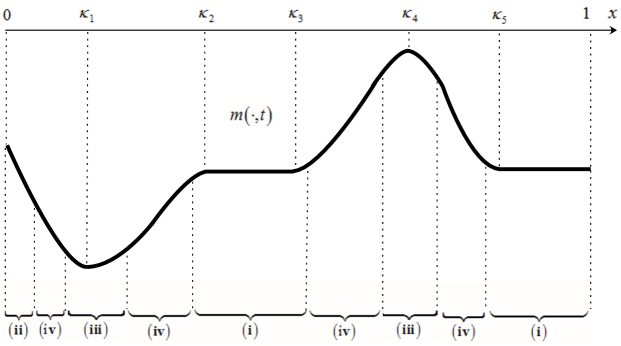
Figure 3. The black solid curve corresponds to an example of $m$ for fixed $t$. The super-solution $\overline{\varphi}$ is constructed respectively on different regions (i)-(v).

(i) On $([\kappa_{i}-\delta,\kappa_{i+1}+\delta]\cap[0,1])\times[0,T]$ for $0\leq i\leq N$ and $i\in\mathbf{B}$ with the small constant $\delta>0$ to be determined later, we define $\overline{\varphi}$ as in the form of (2.58) in Lemma 2.6 with

$$\underline{\kappa}=\kappa_{i}-\delta,\quad\overline{\kappa}=\kappa_{i+1}+\delta,\quad\text{and}\quad c_{1}=c_{2}=\tfrac{1}{2}.$$

(ii) On $([0,\frac{\kappa_{1}}{3}]\cup[\frac{2+\kappa_{N}}{3},1])\times[0,T]$, if $0\not\in\mathbf{B}$ or $N\not\in\mathbf{B}$, then such a super-solution $\overline{\varphi}$ can be constructed by adapting the same arguments as in the proof of Lemma 2.4; Otherwise, it has been constructed in (i).

(iii) On $[\frac{\kappa_{i-1}+2\kappa_{i}}{3},\frac{2\kappa_{i}+\kappa_{i+1}}{3}]\times[0,T]$ for $i\in\mathbf{A}$ and $i-1\in\mathbf{A}$, one constructs $\overline{\varphi}$ by Step 2 of Proposition 2.1 (with $\kappa=\kappa_{i}$) for the case $\partial_{xx}\hat{m}(\kappa_{i})\leq 0$, and by Part II of Proposition 2.3 (with $\kappa=\kappa_{i}$) for the case $\partial_{xx}\hat{m}(\kappa_{i})>0$.

(iv) On the remaining region $\Omega\times[0,T]$, where

$$\Omega=\begin{cases}\vskip 3.0pt plus 1.0pt minus 1.0pt(\frac{2\kappa_{i}+\kappa_{i+1}}{3},\frac{\kappa_{i}+2\kappa_{i+1}}{3})&\text{ for }i\in\mathbf{A}\text{ and }i-1\in\mathbf{A},\\ \vskip 3.0pt plus 1.0pt minus 1.0pt(\kappa_{i-1}+\delta,\frac{2\kappa_{i}+\kappa_{i+1}}{3})&\text{ for }i\in\mathbf{A}\text{ and }i-1\in\mathbf{B},\\ (\frac{\kappa_{i-1}+2\kappa_{i}}{3},\kappa_{i}-\delta)&\text{ for }i\in\mathbf{B},\end{cases}$$

we construct $\overline{\varphi}$ by monotonically connecting the endpoints on $\partial\Omega$, such that

• $\overline{\varphi}$ is continuous at $\partial\Omega\times[0,T]$;

• $|\partial_{x}(\log\overline{\varphi})|>M_{3}$ for some large $M_{3}$;

• $\partial_{x}(\log\overline{\varphi})(x^{+},\cdot)<\partial_{x}(\log\overline{\varphi})(x^{-},\cdot)$ for $x\in\partial\Omega$.

Define $\mathbb{X}=\partial\Omega$. By Lemmas 2.4 and 2.6, explicit calculations as in Propositions 2.1 and 2.3 imply that we may choose $\delta$ smaller if necessary such that the super-solution $\overline{\varphi}$ defined above satisfies (2.24) with $\lambda_{\min}$ being replaced by the right hand side of (1.5). Then the lower bound of $\liminf_{D\rightarrow 0}\lambda(D)$ can be established by Proposition A.1. The proof is now complete. ∎

3. Proof of Theorem 1.2

In this section, we study the case when the ODE (1.4) possesses finite periodic solutions and establish Theorem 1.2 with the help of Theorem 1.3.

Proof of Theorem 1.2.

We first prove part (i) of Theorem 1.2. Let $\{\kappa_{i}\}_{0\leq i\leq N+1}$ be any strictly increasing sequence such that

$$0=\kappa_{0}<\kappa_{1}<\ldots<\kappa_{N}<\kappa_{N+1}=1.$$

Fix small $\delta$ such that $0<\delta<\min\limits_{0\leq i\leq N}(\kappa_{i+1}-\kappa_{i})/3$ and

(3.1) $$\partial_{xx}m\left(x,t\right)\neq 0\quad\text{ for all }\,\,x\in[P_{i}(t)-\delta,P_{i}(t)+\delta],\,t\in[0,T],\,1\leq i\leq N.$$

To “straighten the periodic solution $P_{i}(t)$”, we first define a $C^{2,1}$-diffeomorphism $\Psi:[0,1]\times[0,T]\rightarrow[0,1]$ such that $\partial_{y}\Psi(y,t)\neq 0$ and

(3.2) $$\Psi(y,t)=\begin{cases}\vskip 3.0pt plus 1.0pt minus 1.0pty-\kappa_{i}+P_{i}(t)&\text{ for }y\in[\kappa_{i}-\delta,\kappa_{i}+\delta],\,t\in[0,T],\,1\leq i\leq N,\\ y&\text{ for }y\in[0,\delta]\cup[1-\delta,1],\,t\in[0,T].\end{cases}$$

Define $\widetilde{V}(y,t)=V\left(\Psi(y,t),t\right)$. By direct calculations, $\lambda(D)$ is also the principal eigenvalue of

(3.3) $$\begin{cases}\vskip 6.0pt plus 2.0pt minus 2.0pt\partial_{t}\widetilde{\varphi}-D\frac{\partial_{yy}\widetilde{\varphi}}{(\partial_{y}\Psi)^{2}}-\Big{[}\partial_{y}\widetilde{m}-D\frac{\partial_{yy}\Psi}{(\partial_{y}\Psi)^{3}}\Big{]}\partial_{y}\widetilde{\varphi}+\widetilde{V}(y,t)\widetilde{\varphi}=\lambda(D)\widetilde{\varphi}\ \ &\text{ in }(0,1)\times[0,T],\\ \vskip 6.0pt plus 2.0pt minus 2.0pt\partial_{y}\widetilde{\varphi}(0,t)=\partial_{y}\widetilde{\varphi}(1,t)=0\ \ &\text{ on }[0,T],\\ \widetilde{\varphi}(y,0)=\widetilde{\varphi}(y,T)&\text{ on }(0,1),\end{cases}$$

for which the principal eigenfunction becomes $\widetilde{\varphi}(y,t)=\varphi\left(\Psi(y,t),t\right)$. Here $\varphi$ denotes the principal eigenfunction of problem (1.1), and $\widetilde{m}$ is given by

(3.4) $$\partial_{y}\widetilde{m}(y,t)=\frac{\partial_{x}m\left(\Psi(y,t),t\right)}{\partial_{y}\Psi}+\frac{\partial_{t}\Psi}{\partial_{y}\Psi}.$$

In what follows, we focus on problem (3.3), and divide the proof into several steps.

Step 1. We show that the ODE problem

(3.5) $$\begin{cases}\vskip 3.0pt plus 1.0pt minus 1.0pt\dot{\widetilde{P}}(t)=-\partial_{y}\widetilde{m}(\widetilde{P}(t),t),\\ \widetilde{P}(t)=\widetilde{P}(t+T)\end{cases}$$

has only $N$ periodic solutions $\widetilde{P}_{i}(t)\equiv\kappa_{i}$, and $\partial_{yy}\widetilde{m}\left(y,t\right)\neq 0$ for all $(y,t)\in[\kappa_{i}-\delta,\kappa_{i}+\delta]\times[0,T]$ and $i=1,\ldots,N$.

First, we claim that $\widetilde{P}_{i}(t)\equiv\kappa_{i}$ is a solution of (3.5). This is due to the following calculations:

$$\begin{split}\partial_{y}\widetilde{m}(\kappa_{i},t)&=\frac{\partial_{x}m(\Psi(\kappa_{i},t),t)}{\partial_{y}\Psi(\kappa_{i},t)}+\frac{\partial_{t}\Psi(\kappa_{i},t)}{\partial_{y}\Psi(\kappa_{i},t)}\\ &=\partial_{x}m(P_{i}(t),t)+\dot{P}_{i}(t)=0,\end{split}$$

where the first equality follows from (3.4), and the second equality is due to (3.2).

Suppose on the contrary that there exists a periodic solution $\widetilde{P}(t)$ such that $\widetilde{P}(t)\not\equiv\kappa_{i}$ for any $1\leq i\leq N$. Then by (3.2) and (3.4), one can verify that $\Psi(\widetilde{P}(t),t)\not\equiv P_{i}(t)$ is a periodic solution to (1.4) by the following calculations:

$$\begin{split}\dot{\Psi}(\widetilde{P}(t),t)=\dot{\widetilde{P}}(t)\partial_{y}\Psi+\partial_{t}\Psi&=-\partial_{y}\widetilde{m}(\widetilde{P}(t),t)\partial_{y}\Psi+\partial_{t}\Psi\\ &=-\partial_{x}m(\Psi(\widetilde{P}(t),t),t)-\partial_{t}\Psi+\partial_{t}\Psi\\ &=-\partial_{x}m(\Psi(\widetilde{P}(t),t),t),\end{split}$$

which is a contradiction. Therefore, (3.5) has only $N$ periodic solutions $\widetilde{P}_{i}(t)\equiv\kappa_{i}$ ($i=1,\ldots,N$). Furthermore, from (3.1) and (3.2), it is easily seen that $\partial_{yy}\widetilde{m}\left(y,t\right)\neq 0$ on $[\kappa_{i}-\delta,\kappa_{i}+\delta]\times[0,T]$, which completes Step 1.

In the sequel, we aim to find a proper $C^{2,1}$-transformation $\Phi:[0,1]\times\mathbb{R}\rightarrow[0,1]$ such that $\partial_{z}\Phi>0$, and if for some $\overline{m}\in C^{2,1}([0,1]\times[0,T])$ satisfying

(3.6) $$\partial_{z}\overline{m}(z,r)=\frac{\partial_{y}\widetilde{m}\left(\Phi(z,r),r\right)}{\partial_{z}\Phi}+\frac{\partial_{r}\Phi}{\partial_{z}\Phi},$$

then $\partial_{z}\overline{m}>0$ or $\partial_{z}\overline{m}<0$ holds on $(\kappa_{i},\kappa_{i+1})\times[0,T]$ for each $0\leq i\leq N$. Then we may apply Theorem 1.3 to complete the proof.

Fix any $0\leq i\leq N$. We assume without loss of generality that $\partial_{yy}\widetilde{m}\left(\kappa_{i},t\right)<0$, so that $\partial_{y}\widetilde{m}\left(\kappa_{i}+\delta/2,t\right)<0$. For any $s\in\mathbb{R}$, denote by $q_{s}(t)$ the unique solution of

(3.7) $$\begin{cases}\vskip 3.0pt plus 1.0pt minus 1.0pt\dot{q}(t)=-\partial_{y}\widetilde{m}(q(t),t+s),\\ q(0)=\kappa_{i}+\delta/2,\end{cases}$$

where $\widetilde{m}$ is given by (3.4). Obviously, $q_{s}(t)=q_{s+T}(t)$ for all $s,t\in\mathbb{R}$. We define

(3.8) $$Q(t):=\left\{(q_{r-t}(t),r):r\in\mathbb{R}\right\},$$

which is a continuous curve and is referred as the isochron of (3.7).

Step 2. Fix any $0<t_{1}<t_{2}$. We show that $Q(t_{1})\prec Q(t_{2})$ (see Fig.LABEL:figure2) in the sense that

(3.9) $$q_{r-t_{1}}(t_{1})<q_{r-t_{2}}(t_{2})\quad\text{ for any }\,\,r\in\mathbb{R}.$$

We argue by contradiction by assuming $Q(t_{1})\cap Q(t_{2})\neq\emptyset$ or $Q(t_{2})\prec Q(t_{1})$.

(i) If $Q(t_{1})\cap Q(t_{2})\neq\emptyset$, then by definition (3.8), there exists some $r_{0}\in\mathbb{R}$ such that

(3.10) $$q_{r_{0}-t_{1}}(t_{1})=q_{r_{0}-t_{2}}(t_{2}).$$

Then we define

$$\overline{q}(t):=q_{r_{0}-t_{1}}(t-r_{0}+t_{1})\quad\text{and}\quad\underline{q}(t):=q_{r_{0}-t_{2}}(t-r_{0}+t_{2}),$$

both of which satisfy $\dot{q}(t)=-\partial_{y}\widetilde{m}\left(q(t),t\right)$, and

(3.11) $$\overline{q}(r_{0}-t_{1})=\underline{q}(r_{0}-t_{2})=\kappa_{i}+\delta/2\quad\text{ and }\quad\overline{q}(r_{0})=\underline{q}(r_{0}),$$

where $\overline{q}(r_{0})=\underline{q}(r_{0})$ follows from (3.10). In view of $t_{1}<t_{2}$, we have $r_{0}-t_{1}>r_{0}-t_{2}$. Thanks to the uniqueness of solutions to $\dot{q}(t)=-\partial_{y}\widetilde{m}\left(q(t),t\right)$, we conclude from (3.11) that $\overline{q}(t)=\underline{q}(t)$ for any $t\in[r_{0}-t_{1},r_{0}]$, and particularly, $\underline{q}(r_{0}-t_{1})=\overline{q}(r_{0}-t_{1})=\kappa_{i}+\delta/2=\underline{q}(r_{0}-t_{2})$, i.e. $q_{r_{0}-t_{2}}(t_{2}-t_{1})=\kappa_{i}+\delta/2=q_{r_{0}-t_{2}}(0),$ which contradicts $\partial_{y}\widetilde{m}\left(\kappa_{i}+\delta/2,t\right)<0$.

(ii) If $Q(t_{2})\prec Q(t_{1})$, then given any $(q_{r_{1}-t_{1}}(t_{1}),r_{1})\in Q(t_{1})$, there is some $t_{0}\in(0,t_{1})$ such that $(q_{r_{1}-t_{1}}(t_{0}),r_{2})\in Q(t_{2})$, where $r_{2}=r_{1}-(t_{1}-t_{0})$. By definition (3.8), we also have $(q_{r_{2}-t_{2}}(t_{2}),r_{2})\in Q(t_{2})$, so that $q_{r_{1}-t_{1}}(t_{0})=q_{r_{2}-t_{2}}(t_{2})$. This, together with $r_{2}-t_{0}=r_{1}-t_{1}$, leads to $q_{r_{2}-t_{0}}(t_{0})=q_{r_{2}-t_{2}}(t_{2})$, whence $(q_{r_{2}-t_{2}}(t_{2}),r_{2})\in Q(t_{0})\cap Q(t_{2})$, i.e. $Q(t_{0})\cap Q(t_{2})\neq\emptyset$. Since $t_{0}<t_{2}$, we can apply (i) to reach a contradiction.

Step 3. We show

$$\lim_{t\to\infty}Q(t)=\{(\kappa_{i+1},r):r\in\mathbb{R}\},$$

in the sense that for any $r\in\mathbb{R}$, $q_{r-t}(t)\to\kappa_{i+1}$ as $t\to\infty$.

By $\mathbb{M}$ we denote the set of all continuous curves in $[\kappa_{i}+\delta/2,\kappa_{i+1}]\times[0,T]$. By Step 2, there is some curve $Q_{\infty}:=\{(q_{\infty}(s),s):s\in\mathbb{R}\}\in\mathbb{M}$ such that $Q(t)\to Q_{\infty}$ as $t\to\infty$. It suffices to show $q_{\infty}\equiv\kappa_{i+1}$. To this end, we claim that $q_{\infty}$ is a periodic solution of (3.5), and then $q_{\infty}\equiv\kappa_{i+1}$ is a direct consequence of Step 1.

Indeed, the periodicity of $q_{\infty}$ is due to the fact that $q_{s}(t)=q_{s+T}(t)$ for all $s,t\in\mathbb{R}$. We show that $q_{\infty}$ is a solution to (3.5). Suppose not, then for given $s_{0}\in\mathbb{R}$, there exists some $t_{0}>s_{0}$ such that the unique solution $p_{s_{0}}(t)$ of

$$\begin{cases}\vskip 3.0pt plus 1.0pt minus 1.0pt\dot{p}(t)=-\partial_{y}\widetilde{m}\left(p(t),t+s_{0}\right),\\ p(0)=q_{\infty}(s_{0}),\end{cases}$$

satisfies $p_{s_{0}}(t_{0}-s_{0})\neq q_{\infty}(t_{0})$. Let $t_{*}=t_{0}-s_{0}$. For any $\Sigma_{q}:=\{(q(s),s):s\in\mathbb{R}\}\in\mathbb{M}$, we denote by $p_{s}$ the unique solution of

$$\begin{cases}\vskip 3.0pt plus 1.0pt minus 1.0pt\dot{p}(t)=-\partial_{y}\widetilde{m}\left(p(t),t+s\right),\\ p(0)=q(s),\end{cases}$$

and define a continuous operator $F:\mathbb{M}\to\mathbb{M}$ by

$$F(\Sigma_{q}):=\left\{(p_{s}(t_{*}),t_{*}+s):s\in\mathbb{R}\right\}=\left\{(p_{r-t_{*}}(t_{*}),r):r\in\mathbb{R}\right\}.$$

It is straightforward to verify that $F(Q(t))=Q(t+t_{*})$, and thus

$$F(Q_{\infty})=Q_{\infty},$$

from which we deduce in particular that $p_{t_{0}-t_{*}}(t_{*})=q_{\infty}(t_{0})$, that is $p_{s_{0}}(t_{0}-s_{0})=q_{\infty}(t_{0})$, a contradiction. Therefore, $q_{\infty}$ is a periodic solution of (3.5). Step 3 is thereby completed.

Step 4. We define the transformation $\Phi$ satisfying $\partial_{z}\Phi>0$, and for $\overline{m}$ given by (3.6), we show that $\partial_{z}\overline{m}>0$ or $\partial_{z}\overline{m}<0$ holds in $(\kappa_{i},\kappa_{i+1})\times[0,T]$ for each $0\leq i\leq N$.

For any $0\leq i\leq N$, we define $\Phi_{i}:[\kappa_{i}+\delta/2,\kappa_{i+1}-\delta/2]\times\mathbb{R}\rightarrow[\kappa_{i},\kappa_{i+1}]$ such that for any $(z,r)\in[\kappa_{i}+\delta,\kappa_{i+1}-\delta]\times\mathbb{R}$,

(3.12) $$\Phi_{i}(z,r)=q_{r-\tau_{i}(z)}(\tau_{i}(z)),$$

where $q_{r-\tau_{i}(z)}$ is the solution of (3.7) with $s=r-\tau_{i}(z)$ and $\tau_{i}(z)$ is determined by

(3.13) $$q_{-\tau_{i}(z)}(\tau_{i}(z))=z.$$

Obviously, $\{(\Phi_{i}(z,r),r):r\in\mathbb{R}\}=Q(\tau_{i}(z))$. It is easily seen that $z\to\tau_{i}(z)$ is a bijection (where the surjection follows from Step 3), is of class $C^{2}$ and is increasing (by Step 2), so that $\Phi_{i}\in C^{2,1}([\kappa_{i}+\delta,\kappa_{i+1}-\delta]\times\mathbb{R})$ and $\partial_{z}\Phi_{i}\geq 0$ by (3.9).

We claim that for $(z,r)\in(\kappa_{i}+\delta/2,\kappa_{i+1}-\delta/2)\times\mathbb{R}$,

(3.14) $$\tau^{\prime}_{i}(z)>0\quad\text{and}\quad\partial_{y}\widetilde{m}\left(\Phi_{i}(z,r),r\right)+\partial_{r}\Phi_{i}=-\frac{\partial_{z}\Phi_{i}}{\tau^{\prime}_{i}(z)}.$$

For the sake of clarification, write $q_{s}(t)=q(t;s)$, where $q_{s}$ is defined by (3.7). Differentiating both sides of (3.13) by $z$, we derive that

$$\Big{[}\partial_{t}q_{-\tau_{i}(z)}(\tau_{i}(z))-\partial_{s}q_{-\tau_{i}(z)}(\tau_{i}(z))\Big{]}\tau^{\prime}_{i}(z)=1,$$

which implies $\tau^{\prime}_{i}(z)\neq 0$, and thus $\tau^{\prime}_{i}(z)>0$ since $\tau_{i}(z)$ is increasing. Similarly, by (3.12), we deduce that $\partial_{r}\Phi_{i}(z,r)=\partial_{s}q_{r-\tau_{i}(z)}(\tau_{i}(z))$, and thus

(3.15) $$\begin{split}\partial_{z}\Phi_{i}(z,r)&=\Big{[}\partial_{t}q_{r-\tau_{i}(z)}(\tau_{i}(z))-\partial_{s}q_{r-\tau_{i}(z)}(\tau_{i}(z))\Big{]}\tau^{\prime}_{i}(z)\\ &=\Big{[}\partial_{t}q_{r-\tau_{i}(z)}(\tau_{i}(z))-\partial_{r}\Phi_{i}(z,r)\Big{]}\tau^{\prime}_{i}(z).\end{split}$$

By the definition of $q_{r-\tau_{i}(z)}(\tau_{i}(z))$ in (3.7) with $s=r-\tau_{i}(z)$ and $t=\tau_{i}(z)$, we note that

$$\partial_{t}q_{r-\tau_{i}(z)}(\tau_{i}(z))=-\partial_{y}\widetilde{m}(\Phi_{i}(z,r),r),$$

which, together with (3.15), implies (3.14).

We then claim that

(3.16) $$\partial_{z}\Phi_{i}(z,r)>0\quad\text{for any}\quad(z,r)\in(\kappa_{i}+\delta/2,\kappa_{i+1}-\delta/2)\times\mathbb{R}.$$

To this end, denote by $\tilde{p}(t;s)$ the unique solution of the problem

$$\begin{cases}\vskip 3.0pt plus 1.0pt minus 1.0pt\dot{\tilde{p}}(t)=-\partial_{y}\widetilde{m}\left(\tilde{p}(t),t\right),\\ \tilde{p}(s)=\kappa_{i}+\delta/2,\end{cases}$$

whence by (3.7), we observe that $q_{s}(t)=\tilde{p}(t+s;s)$. For any $\tau\in\mathbb{R}$, we have

$$\tilde{p}(\tau)=-\int_{s}^{\tau}\partial_{y}\widetilde{m}\left(\tilde{p}(t),t\right)\mathrm{d}t+\kappa_{i}+\delta/2,$$

so that

$$\partial_{s}\tilde{p}(\tau)=\partial_{y}\widetilde{m}\left(\kappa_{i}+\delta/2,s\right)-\int_{s}^{\tau}\partial_{yy}\widetilde{m}\left(\tilde{p}(t),t\right)\partial_{s}\tilde{p}(t)\mathrm{d}t,$$

and thus $\partial_{s}\tilde{p}(s)=\partial_{y}\widetilde{m}\left(\kappa_{i}+\delta/2,s\right)<0$. We further calculate that

$$\partial_{\tau}\left(\partial_{s}\tilde{p}(\tau)\right)=-\partial_{yy}\widetilde{m}\left(\tilde{p}(\tau),\tau\right)\partial_{s}\tilde{p}(\tau),$$

which implies immediately that for any $r\in\mathbb{R}$,

(3.17) $$\partial_{s}\tilde{p}(r)=\partial_{s}\tilde{p}(s)\exp\left[-\int_{s}^{r}\partial_{yy}\widetilde{m}\left(\tilde{p}(\tau),\tau\right)\mathrm{d}\tau\right]<0.$$

By (3.12) and the fact that $q_{s}(t)=\tilde{p}(t+s;s)$, we can see $\Phi_{i}(z,r)=\tilde{p}(r;r-\tau_{i}(z))$, so that

$$\partial_{z}\Phi_{i}(z,r)=-\partial_{s}\tilde{p}(r)\cdot\tau^{\prime}_{i}(z)>0$$

by noting that $\tau^{\prime}_{i}(z)>0$ in (3.14) and $\partial_{s}\tilde{p}(r)<0$ in (3.17).

Then we define a $C^{2,1}$-transformation $\Phi:[0,1]\times\mathbb{R}\rightarrow[0,1]$ such that $\partial_{z}\Phi>0$ and for any $0\leq i\leq N$,

(3.18) $$\Phi(z,r):=\begin{cases}\vskip 3.0pt plus 1.0pt minus 1.0pt\Phi_{i}(z,r)&\text{ on }[\kappa_{i}+\delta_{1},\kappa_{i+1}-\delta_{1}]\times\mathbb{R},\\ z&\text{ on }\left([\kappa_{i},\kappa_{i}+\delta/2]\cup[\kappa_{i+1}-\delta/2,\kappa_{i+1}]\right)\times\mathbb{R},\\ \end{cases}$$

where $\delta_{1}\in(\delta/2,\delta]$ is chosen to be close to $\delta/2$ such that

(3.19) $$\partial_{y}\widetilde{m}+\partial_{r}\Phi<0\,\,\,\,\text{ on }\,\,\left([\kappa_{i},\kappa_{i}+\delta_{1}]\cup[\kappa_{i+1}-\delta_{1},\kappa_{i+1}]\right)\times\mathbb{R}.$$

This is possible since by (3.18) and Step 1, it follows that

$$\partial_{y}\widetilde{m}+\partial_{r}\Phi=\partial_{y}\widetilde{m}<0\,\,\text{ on }\left([\kappa_{i},\kappa_{i}+\delta/2]\cup[\kappa_{i+1}-\delta/2,\kappa_{i+1}]\right)\times\mathbb{R}.$$

Let $\overline{m}$ satisfy (3.6) with $\Phi$ defined by (3.18). For any $z\in[\kappa_{i},\kappa_{i}+\delta_{1}]\cup[\kappa_{i+1}-\delta_{1},\kappa_{i+1}]$, it follows from (3.6), (3.18), and (3.19) that $\partial_{z}\overline{m}(z,r)<0$; For $z\in[\kappa_{i}+\delta_{1},\kappa_{i+1}-\delta_{1}]$, by (3.18) we have $\Phi(z,r)=\Phi_{i}(z,r)$, whence comparing (3.6) with (3.14) gives $\partial_{z}\overline{m}(z,r)=-\frac{1}{\tau^{\prime}_{i}(z)}<0$. This completes Step 4.

Step 5. We apply Theorem 1.3 to complete the proof. Let the $C^{2,1}$-transformation $\Phi$ be defined by (3.18) in Step 4. Denote

$$\overline{V}(z,r):=\widetilde{V}\left(\Phi(z,r),r\right)\quad\text{ and }\quad\overline{\varphi}(z,r):=\widetilde{\varphi}\left(\Phi(z,r),r\right),$$

where $\widetilde{V}$ and $\widetilde{\varphi}$ are defined in (3.3). Using the definition of $\overline{m}$ in (3.6), direct calculation enables us to transform (3.3) into the following equation:

(3.20) $$\begin{cases}\begin{array}[]{l}\vskip 3.0pt plus 1.0pt minus 1.0pt\partial_{r}\overline{\varphi}-\frac{D\partial_{zz}\overline{\varphi}}{(\partial_{y}\Psi)^{2}(\partial_{z}\Phi)^{2}}-\Big{[}\partial_{z}\overline{m}+D\eta_{3}\Big{]}\partial_{z}\overline{\varphi}+\overline{V}\overline{\varphi}=\lambda(D)\overline{\varphi}\end{array}\ \ &\text{ in }(0,1)\times[0,T],\\ \vskip 6.0pt plus 2.0pt minus 2.0pt\partial_{z}\overline{\varphi}(0,r)=\partial_{z}\overline{\varphi}(1,r)=0\ \ &\text{ on }[0,T],\\ \overline{\varphi}(z,0)=\overline{\varphi}(z,T)&\text{ on }(0,1),\end{cases}$$

where $\eta_{3}$ is given by

$$\eta_{3}(z,r):=\frac{\partial_{yy}\Psi}{(\partial_{y}\Psi)^{3}\partial_{z}\Phi}+\frac{\partial_{zz}\Phi}{(\partial_{z}\Phi)^{3}(\partial_{y}\Psi)^{2}}.$$

For each $0\leq i\leq N$, by Step 4, $\partial_{z}\overline{m}>0$ or $\partial_{z}\overline{m}<0$ holds for all $z\in(\kappa_{i},\kappa_{i+1})$; by the definitions of $\Psi$ and $\Phi$ in (3.2) and (3.18), we find that for any $z\in[\kappa_{i},\kappa_{i}+\delta/2]\cup[\kappa_{i+1}-\delta/2,\kappa_{i+1}]$, $\partial_{yy}\Psi=\partial_{zz}\Phi=0$, so that $\eta_{3}(z,r)=0$. Therefore, we conclude that for any small $\vartheta>0$, there exists some $\epsilon_{0}=\epsilon_{0}(\vartheta)>0$, independent of small $D$, such that

(3.21) $$\partial_{z}\overline{m}+D\eta_{3}\geq\epsilon_{0}\quad\text{or}\quad\partial_{z}\overline{m}+D\eta_{3}\leq-\epsilon_{0}\quad\text{on}\,\,\,[\kappa_{i}+\vartheta,\kappa_{i+1}-\vartheta]\times[0,T].$$

Moreover, from (3.6) and (3.18), we observe that for any $1\leq i\leq N$,

$$\partial_{z}\overline{m}(\kappa_{i},r)=\partial_{y}\widetilde{m}\left(\Phi(\kappa_{i},r),r\right)=\partial_{y}\widetilde{m}\left(\kappa_{i},r\right)=0,$$

which implies that $\partial_{z}\overline{m}(\kappa_{i},r)+D\eta_{3}(\kappa_{i},r)=0$ since $\eta_{3}(\kappa_{i},r)=0$. Together with (3.21), noting that $\partial_{y}\Psi=\partial_{z}\Phi=1$ on $[\kappa_{i},\kappa_{i}+\tilde{\vartheta}]\cup[\kappa_{i+1}-\tilde{\vartheta},\kappa_{i+1}]$ with some $0<\tilde{\vartheta}\ll 1$ for any $0\leq i\leq N$, we can follow directly the same proof of Theorem 1.3 with $\mathbf{B}=\emptyset$ to (3.20) and deduce that

(3.22) $$\lim_{D\rightarrow 0}\lambda(D)=\min_{0\leq i\leq N+1}\left\{\hat{\overline{V}}(\kappa_{i})+[\partial_{xx}\hat{m}]_{+}(\kappa_{i})\right\}.$$

Noting that $\hat{\overline{V}}(\kappa_{i})=\frac{1}{T}\int_{0}^{T}V\left(P_{i}(s),s\right)\mathrm{d}s$ and

$$\partial_{zz}\overline{m}(\kappa_{i},r)=\partial_{yy}\widetilde{m}\left(\kappa_{i},r\right)=\partial_{xx}m\left(P_{i}(r),r\right),$$

part (i) of Theorem 1.2 follows from (3.22).

Finally, part (ii) of Theorem 1.2 can be established by Steps 2-5 with $N=0$. The proof is now complete. ∎

4. Proof of Theorem 1.4

This section is devoted to the case $m(x,t)=\alpha b(t)x$ and the proof of Theorem 1.4. We start with the existence and uniqueness of $\tilde{P}_{\alpha}$ defined in Theorem 1.4.

Lemma 4.1.

Let $F$ be defined by (1.7) and $\overline{P}$,$\underline{P}$ be given in Theorem 1.4. If $\alpha\geq\frac{1}{\overline{P}-\underline{P}}$, then

(4.1) $$\begin{cases}\vskip 3.0pt plus 1.0pt minus 1.0pt\dot{P}(t)=-\alpha F\left(P(t),t\right),\\ P(t)=P(t+T)\end{cases}$$

has a unique $T$-periodic solution in $W^{1,\infty}(\mathbb{R})$.

Proof.

Recalling the definition of $F$ in (1.7), we observe that $F(0,t)=\min\{b(t),0\}\leq 0$ and $F(1,t)=\max\{b(t),0\}\geq 0$, so that $P_{*}\equiv 0$ and $P^{*}\equiv 1$ are a pair of sub- and super-solutions to (4.1). Hence, as $F$ is bounded, there exists at least one $T$-periodic solution in $W^{1,\infty}(\mathbb{R})$.

For the uniqueness, given any two $T$-periodic solutions $\tilde{P}$ and $\tilde{P}_{\alpha}$ of (4.1), we show $\tilde{P}=\tilde{P}_{\alpha}$. Suppose not, without loss of generality we may assume $\tilde{P}(0)<\tilde{P}_{\alpha}(0)$. We consider two cases:

(i) If $\tilde{P}(t_{1})=\tilde{P}_{\alpha}(t_{1})$ for some $t_{1}\in(0,T)$, in view of $\tilde{P}(T)=\tilde{P}(0)<\tilde{P}_{\alpha}(0)=\tilde{P}_{\alpha}(T)$, by continuity there is some $\tilde{t}_{1}\in[t_{1},T)$ such that $\tilde{P}(\tilde{t}_{1})=\tilde{P}_{\alpha}(\tilde{t}_{1})$ and $\tilde{P}(t)<\tilde{P}_{\alpha}(t)$ for any $t\in(\tilde{t}_{1},T]$. Then by the definition of $F$, it can be verified that for any $t\in[\tilde{t}_{1},T]$,

(4.2) $$[\tilde{P}_{\alpha}(t)-\tilde{P}(t)]-[\tilde{P}_{\alpha}(\tilde{t}_{1})-\tilde{P}(\tilde{t}_{1})]=\alpha\int_{\tilde{t}_{1}}^{t}\left[F(\tilde{P}(s),s)-F(\tilde{P}_{\alpha}(s),s)\right]\,ds\leq 0,$$

which implies $\tilde{P}_{\alpha}(T)-\tilde{P}(T)\leq\tilde{P}_{\alpha}(\tilde{t}_{1})-\tilde{P}(\tilde{t}_{1})=0$, a contradiction.

(ii) If $\tilde{P}(t)<\tilde{P}_{\alpha}(t)$ for all $t\in[0,T]$, then (4.2) holds for all $t\in[0,T]$ and $\tilde{t}_{1}=0$. In view of $\tilde{P}_{\alpha}(T)-\tilde{P}(T)=\tilde{P}_{\alpha}(0)-\tilde{P}(0)$, we deduce that

$$\tilde{P}_{\alpha}(t)-\tilde{P}(t)\equiv\tilde{P}_{\alpha}(0)-\tilde{P}(0)\quad\text{for all}\quad t\in[0,T].$$

In such a case, again by the definition of $F$, we infer that

$$\tilde{P}_{+}:=\tilde{P}+(\tilde{P}_{\alpha}(0)-\tilde{P}(0))/2\in(0,1)$$

defines a $T$-periodic solution of (4.1), and thus $\dot{\tilde{P}}_{+}=-\alpha b(t)$, where $\tilde{P}_{+}\in(0,1)$ is due to $0\leq\tilde{P}<\tilde{P}_{+}<\tilde{P}_{\alpha}\leq 1$. By recalling $P(t)=-\int_{0}^{t}b(s)\mathrm{d}s$, this implies that $\tilde{P}_{+}=\alpha P(t)+c\in(0,1)$ for some constant $c\in\mathbb{R}$, so that

$$1>\max_{[0,T]}\tilde{P}_{+}-\min_{[0,T]}\tilde{P}_{+}=\alpha(\overline{P}-\underline{P}),$$

which contradicts $\alpha\geq\frac{1}{\overline{P}-\underline{P}}$. Lemma 4.1 thus follows. ∎

We are now ready to prove Theorem 1.4.

Proof of Theorem 1.4.

The proof is divided into three steps.

Step 1. Assume $\hat{b}\neq 0$ and show part (i) of Theorem 1.4. Let $\Psi_{1}:[0,1]\times[0,T]\rightarrow\mathbb{R}$ denote a $T$-periodic diffeomorphism given by

$$\Psi_{1}(y,t)=\alpha\left[\hat{b}t-\int_{0}^{t}b(s)\,\mathrm{d}s\right]+y.$$

Under the transformation $x=\Psi_{1}(y,t)$, as in (3.3), direct calculation from (1.6) yields that $\lambda(D)$ defines the principal eigenvalue of the problem

$$\begin{cases}\vskip 3.0pt plus 1.0pt minus 1.0pt\partial_{t}\varphi-D\partial_{yy}\varphi-\alpha\hat{b}\cdot\partial_{y}\varphi+V_{1}\varphi=\lambda(D)\varphi,\ \ &y\in(-\Psi_{1}(0,t),1-\Psi_{1}(0,t)),t\in[0,T],\\ \vskip 3.0pt plus 1.0pt minus 1.0pt\partial_{y}\varphi(-\Psi_{1}(0,t),t)=\partial_{y}\varphi(1-\Psi_{1}(0,t),t)=0,\ \ &t\in[0,T],\\ \varphi(y,0)=\varphi(y,T),&y\in[-\Psi_{1}(0,0),1-\Psi_{1}(0,0)],\end{cases}$$

where $V_{1}(y,t)=V\left(\Psi_{1}(y,t),t\right)$. Then we can conclude that part (i) of Theorem 1.4 is a direct consequence of Theorem 1.2. Indeed, if $\hat{b}>0$ for example, then ODE (1.4) with $\partial_{x}m=\alpha\hat{b}>0$ has no periodic solutions, so that by part (ii) of Theorem 1.2 we deduce that

$$\lim_{D\to 0}\lambda(D)=\frac{1}{T}\int_{0}^{T}V_{1}(1-\Psi_{1}(0,s),s)\mathrm{d}s=\hat{V}(1).$$

The same argument can be adapted to the case $\hat{b}<0$, which completes Step 1.

Step 2. Assume $\hat{b}=0$ and $0<\alpha\leq\frac{1}{\overline{P}-\underline{P}}$. We prove the first part of (ii) in Theorem 1.4. Recall $P(t)=-\int_{0}^{t}b(s)\mathrm{d}s$ defined in Theorem 1.4. Taking the transformation $x=y+\alpha P(t)$ in (1.6), we derive that $\lambda(D)$ is also the principal eigenvalue of the problem

$$\begin{cases}\vskip 3.0pt plus 1.0pt minus 1.0pt\partial_{t}\varphi-D\partial_{yy}\varphi+V_{2}\varphi=\lambda(D)\varphi,\ \ &y\in(-\alpha P(t),1-\alpha P(t)),\,t\in[0,T],\\ \vskip 3.0pt plus 1.0pt minus 1.0pt\partial_{y}\varphi(-\alpha P(t),t)=\partial_{y}\varphi(1-\alpha P(t),t)=0,\ \ &t\in[0,T],\\ \varphi(y,0)=\varphi(y,T),&y\in(-\alpha P(0),1-\alpha P(0)),\end{cases}$$

where $V_{2}(y,t)=V\left(\alpha P(t)+y,t\right)$. Under the transformation $x=y+\alpha P(t)$, all periodic solutions of (1.4) are constants in the interval $[-\alpha\underline{P},1-\alpha\overline{P}]$. This includes the special case $\alpha=\frac{1}{\overline{P}-\underline{P}}$, for which the interval reduces to a single point. It is desired to show that

$$\lim\limits_{D\rightarrow 0}\lambda(D)=\min_{y\in[-\alpha\underline{P},\,1-\alpha\overline{P}]}\hat{V}_{2}(y).$$

First, the upper bound $\limsup_{D\rightarrow 0}\lambda(D)\leq\hat{V}_{2}(y)$, for any $y\in[-\alpha\underline{P},1-\alpha\overline{P}]$, can be established by the same arguments as in Step 1 of Lemma 2.6 by constructing the sub-solution locally. We thus omit the details here.

It remains to show the lower bound of $\liminf_{D\rightarrow 0}\lambda(D)$. For any $\epsilon>0$, we define $T$-periodic function $V_{2\epsilon}\in C^{2,1}(\mathbb{R}\times[0,T])$ satisfying $\|V_{2\epsilon}-V_{2}\|_{L^{\infty}}\leq\epsilon$, and choose small $\delta>0$ such that

(4.3) $$\tilde{\lambda}_{\rm min}:=\min_{y\in[-\alpha\underline{P}-2\delta,1-\alpha\overline{P}+2\delta]}\hat{V}_{2\epsilon}(y)\geq\min_{y\in[-\alpha\underline{P},1-\alpha\overline{P}]}\hat{V}_{2}(y)-2\epsilon.$$

We define $\overline{\phi}\in C^{2,1}([-\alpha\underline{P}-2\delta,\,1-\alpha\overline{P}+2\delta]\times[0,T])$ by

(4.4) $$\overline{\phi}(y,t):=\mbox{exp}\left[-\int_{0}^{t}V_{2\epsilon}(y,s)\mathrm{d}s+t\hat{V}_{2\epsilon}(y)\right]\beta_{\epsilon}(y),$$

where $\beta_{\epsilon}\in C^{2}([-\alpha\underline{P}-2\delta,\,1-\alpha\overline{P}+2\delta])$ is a positive function chosen such that

(4.5) $$\partial_{y}\overline{\phi}<0\,\,\text{ on }[-\alpha\underline{P}-2\delta,-\alpha\underline{P}]\times[0,T]\quad\text{and}\quad\partial_{y}\overline{\phi}>0\,\,\text{ on }[1-\alpha\overline{P},1-\alpha\overline{P}+2\delta]\times[0,T].$$

Next, we aim to find a super-solution $\overline{\varphi}\in C([0,1]\times[0,T])$ which satisfies

(4.6) $$\begin{cases}\vskip 3.0pt plus 1.0pt minus 1.0pt\partial_{t}\overline{\varphi}-D\partial_{yy}\overline{\varphi}+V_{2}\overline{\varphi}\geq\left[\tilde{\lambda}_{\rm min}-3\epsilon\right]\overline{\varphi},&y\in(-\alpha P(t),1-\alpha P(t))\backslash\mathbb{X},\,t\in[0,T],\\ \vskip 3.0pt plus 1.0pt minus 1.0pt\partial_{y}\overline{\varphi}(-\alpha P(t),t)\leq 0\leq\partial_{y}\overline{\varphi}(1-\alpha P(t),t),&t\in[0,T],\\ \overline{\varphi}(y,0)=\overline{\varphi}(y,T),&y\in(-\alpha P(0),1-\alpha P(0)),\end{cases}$$

where $\mathbb{X}=\{-\alpha\underline{P}-2\delta,\,1-\alpha\overline{P}+2\delta\}$. Then it follows from Proposition A.1 and (4.3) that

$$\liminf\limits_{D\rightarrow 0}\lambda(D)\geq\min_{y\in[-\alpha\underline{P},\,1-\alpha\overline{P}]}\hat{V}_{2}(y);$$

see also Remark A.1.

We only construct $\overline{\varphi}$ for $y\in(-\alpha P(t),1-\alpha\overline{P}+\delta)$ and $t\in[0,T]$. The constructions of the remaining regions are similar. To this end, by the definition of $\underline{P}$, there exist $t_{3}>t_{2}$ such that

$$[t_{2},t_{3}]\subset\{t\in[0,T]:-\alpha P(t)>-\alpha\underline{P}-\delta\}.$$

We then choose $\eta_{4}\in C^{2,1}((-\infty,1-\alpha\overline{P}+\delta]\times[0,T])$ to be a positive $T$-periodic function, and satisfy that $\partial_{y}\eta_{4}\leq 0$ and

(4.7) $$\begin{cases}\vskip 6.0pt plus 2.0pt minus 2.0pt\eta_{4}\equiv 1&\text{on }[-\alpha\underline{P}-\delta,\,1-\alpha\overline{P}+\delta]\times[0,T],\\ \vskip 6.0pt plus 2.0pt minus 2.0pt\partial_{t}(\log\eta_{4})>0&\text{on }[-\alpha\underline{P}-2\delta,-\alpha\underline{P}-\delta)\times\left([0,T]\setminus[t_{2},t_{3}]\right),\\ \partial_{t}(\log\eta_{4})\geq M_{4}&\text{on }(-\infty,-\alpha\underline{P}-2\delta]\times\left([0,T]\setminus[t_{2},t_{3}]\right).\end{cases}$$

Here $M_{4}$ is chosen such that

$$M_{4}>\|V_{2}\|_{L^{\infty}}+\tilde{\lambda}_{\rm min}+\|\partial_{t}\log\overline{\phi}\|_{L^{\infty}},$$

where $\overline{\phi}$ is defined by (4.4). Moreover, we extend $\overline{\phi}$ to $(-\infty,1-\alpha\underline{P}+2\delta]\times[0,T]$ by setting $\overline{\phi}(\cdot,t)\equiv\overline{\phi}(-\alpha\underline{P}-2\delta,t)$ on $(-\infty,-\alpha\underline{P}-2\delta)\times[0,T]$, so that by (4.5) we have

(4.8) $$\partial_{y}\overline{\phi}((-\alpha\underline{P}-2\delta)^{+},\cdot)<0=\partial_{y}\overline{\phi}((-\alpha\underline{P}-2\delta)^{-},\cdot).$$

Let $\overline{\phi}$ and $\eta_{4}$ be given by (4.4) and (4.7), then we define

(4.9) $$\overline{\varphi}(y,t):=\eta_{4}(y,t)\cdot\overline{\phi}(y,t).$$

By (4.8), as $\eta_{4}$ is smooth, one can infer that

$$\partial_{y}\log\overline{\varphi}\left((-\alpha\underline{P}-2\delta)^{+},\cdot\right)<\partial_{y}\log\overline{\varphi}\left((-\alpha\underline{P}-2\delta)^{-},\cdot\right)\quad\text{as }\,-\alpha\underline{P}-2\delta\in\mathbb{X}.$$

It remains to check that $\overline{\varphi}$ defined above satisfies (4.6).

(i) For $y\in(-\alpha P(t),1-\alpha P(t))\cap[-\alpha\underline{P}-\delta,1-\alpha\overline{P}+\delta]$ and $t\in[0,T]$, since $\eta_{4}\equiv 1$ in (4.7), we have $\overline{\varphi}(y,t)=\overline{\phi}(y,t)$. By the definition of $\overline{\phi}$ in (4.4), direct calculations yield that

$$\begin{split}\vskip 3.0pt plus 1.0pt minus 1.0pt\partial_{t}\overline{\varphi}-D\partial_{yy}\overline{\varphi}+V_{2}\overline{\varphi}&=\left[\hat{V}_{2\epsilon}(y)-V_{2\epsilon}(y,t)+V_{2}(y,t)\right]\overline{\phi}-D\partial_{yy}\overline{\phi}.\end{split}$$

By the definition of $V_{2\epsilon}$, we can argue as in Lemma 2.6 to choose $D$ small such that the first inequality in (4.6) holds. Then the part of boundary conditions on $\{-\alpha P(t),1-\alpha P(t)\}\cap[-\alpha\underline{P}-\delta,1-\alpha\overline{P}+\delta]$ and $t\in[0,T]$ can be verified by (4.5).

(ii) For $y\in(-\alpha P(t),1-\alpha P(t))\cap[-\alpha\underline{P}-2\delta,-\alpha\underline{P}-\delta)$ and $t\in[0,T]$, since $t\in[0,T]\setminus[t_{2},t_{3}]$ in this case, we use (4.7) and (4.9) to deduce that

$$\begin{split}\partial_{t}\overline{\varphi}-D\partial_{yy}\overline{\varphi}+V_{2}\overline{\varphi}&=\left[\hat{V}_{2\epsilon}(y)-V_{2\epsilon}(y,t)+V_{2}(y,t)\right]\overline{\varphi}+\left[\partial_{t}(\log\eta_{4})-D\partial_{yy}\overline{\varphi}\right]\overline{\varphi}\\ &\geq\left[\tilde{\lambda}_{\rm min}-2\epsilon+\partial_{t}(\log\eta_{4})+O(D)\right]\overline{\varphi}.\end{split}$$

Since $\partial_{t}(\log\eta_{4})>0$ in this case, again we choose $D$ small such that (4.6) holds. And the boundary conditions in this case can be verified by $\partial_{y}\overline{\phi}\leq 0$ and $\partial_{y}\eta_{4}\leq 0$.

(iii) For $y\in(-\alpha P(t),1-\alpha P(t))\cap(-\infty,-\alpha\underline{P}-2\delta)$ and $t\in[0,T]$, since $\overline{\phi}$ is independent of $y$, by (4.7) and (4.9) direct calculation yields that

$$\begin{split}\partial_{t}\overline{\varphi}-D\partial_{yy}\overline{\varphi}+V_{2}\overline{\varphi}\geq\Big{[}(\log\overline{\phi})^{\prime}+M_{4}-D\partial_{yy}\eta_{4}/\eta_{4}+V_{2}\Big{]}\overline{\varphi}.\end{split}$$

Thus the first inequality in (4.6) is verified by the definition of $M_{4}$, and the boundary condition follows from $\partial_{y}\eta_{4}\leq 0$. Step 2 is now completed.

Step 3. Assume $\hat{b}=0$ and $\alpha>\frac{1}{\overline{P}-\underline{P}}$. We establish the second part of (ii) in Theorem 1.4. Let $\tilde{P}_{\alpha}$ denote the unique solution of (4.1). We apply the transformation $x=y+\tilde{P}_{\alpha}(t)$ to rewrite problem (1.6) as

$$\begin{cases}\vskip 6.0pt plus 2.0pt minus 2.0pt\partial_{t}\varphi-D\partial_{yy}\varphi-\alpha\tilde{b}(t)\partial_{y}\varphi+V_{3}\varphi=\lambda(D)\varphi,\ \ &(y,t)\in\tilde{\Omega},\\ \vskip 6.0pt plus 2.0pt minus 2.0pt\partial_{y}\varphi(-\tilde{P}_{\alpha}(t),t)=\partial_{y}\varphi(1-\tilde{P}_{\alpha}(t),t)=0,\ \ &t\in[0,T],\\ \varphi(y,0)=\varphi(y,T),&y\in(-\tilde{P}_{\alpha}(0),1-\tilde{P}_{\alpha}(0)),\end{cases}$$

where $\tilde{b}(t):=b(t)-F(\tilde{P}_{\alpha}(t),t)$, $V_{3}(y,t)=V(\tilde{P}_{\alpha}(t)+y,t)$, and

$$\tilde{\Omega}=\left\{(y,t):y\in(-\tilde{P}_{\alpha}(t),1-\tilde{P}_{\alpha}(t)),\,t\in[0,T]\right\}.$$

See Fig.4 for an example of this transformation.

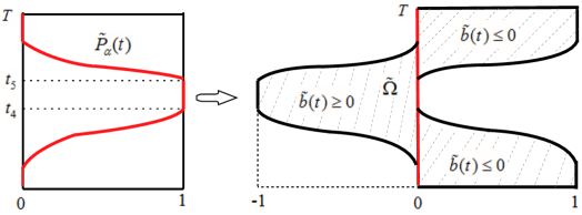
Figure 4. The diagram of $\tilde{\Omega}$ under transformation $x=y+\tilde{P}_{\alpha}(t)$. The red colored curve in the left side picture corresponds to $\tilde{P}_{\alpha}(t)$, whereas the red colored line in the right side picture is the image of $\tilde{P}_{\alpha}(t)$ after the transformation.

It remains to prove

$$\lim\limits_{D\rightarrow 0}\lambda(D)=\hat{V}_{3}(0).$$

The upper bound $\limsup_{D\rightarrow 0}\lambda(D)\leq\hat{V}_{3}(0)$ can be established by using the arguments in Step 1 of Proposition 2.1. We next prove $\liminf_{D\rightarrow 0}\lambda(D)\geq\hat{V}_{3}(0)$.

We claim that if $\alpha>\frac{1}{\overline{P}-\underline{P}}$, then

$$\mathrm{mes}\Big{\{}t\in[0,T]:\tilde{P}_{\alpha}(t)\in\{0,1\}\,\text{ and }\,b\neq 0\Big{\}}>0,$$

i.e. there exist $0\leq t_{4}<t_{5}\leq T$ such that $b\neq 0$, and $\tilde{P}_{\alpha}(t)\equiv 0$ or $\tilde{P}_{\alpha}(t)\equiv 1$ on $[t_{4},t_{5}]$. Suppose not, then $\tilde{P}_{\alpha}$ is also a periodic solution of $\dot{P}(t)=-\alpha b(t)$, so that $\tilde{P}_{\alpha}(t)=P(t)+c$ for $c\in\mathbb{R}$, where $P(t)=-\int_{0}^{t}b(s)\mathrm{d}s$ as defined in part (ii) of Theorem 1.4. Since $\tilde{P}_{\alpha}\in[0,1]$, we have

$$1\geq\max_{[0,T]}\tilde{P}_{\alpha}-\min_{[0,T]}\tilde{P}_{\alpha}=\alpha(\overline{P}-\underline{P}),$$

which contradicts $\alpha>\frac{1}{\overline{P}-\underline{P}}$.

In what follows, we assume $\tilde{P}_{\alpha}(t)\equiv 1$ on $[t_{4},t_{5}]$, and the proof is similar for the other case. To proceed further, we introduce positive functions $\overline{z}_{5}\in C^{2}(\mathbb{R})$ and $\eta_{5}\in C^{1}([0,T])$ as follows: For any $\epsilon>0$, we choose some small $\delta>0$ such that

(4.10) $$\begin{array}[]{ll}|V_{3}(y,t)-V_{3}(0,t)|<\epsilon/2\,\,\text{ on }\,[-2\delta,2\delta]\times[0,T].\end{array}$$

We first choose $\eta_{5}$ to be $T$-periodic and

(4.11) $$(\log\eta_{5})^{\prime}>2\|V\|_{L^{\infty}}+\|(\log f_{1})^{\prime}\|_{L^{\infty}}\quad\text{on }\,\,[0,t_{4}+\delta]\cup[t_{5}-\delta,T].$$

Then we choose $\overline{z}_{5}$ such that

(4.12) $$\begin{cases}\vskip 3.0pt plus 1.0pt minus 1.0pt\overline{z}_{5}^{\prime}(y)<0\,\,\text{ in }\,(-\infty,0),\,\,\,\,\overline{z}_{5}^{\prime}(y)>0\,\,\text{ in }\,(0,\infty),\\ (\log\overline{z}_{5})^{\prime}\leq-M_{5}\,\,\text{ in }\,(-\infty,-\delta),\end{cases}$$

where $M_{5}$ is some large constant to be determined later.

We define

(4.13) $$\overline{\varphi}(y,t):=\overline{z}_{5}(y)\cdot\begin{cases}f_{1}(t)&\text{for }|y|\leq\delta,\\ \zeta_{5}(y,t)&\text{for }-2\delta<y<-\delta,\\ \zeta_{5}(-y,t)&\text{for }\delta<y<2\delta,\\ \eta_{5}(t)&\text{for }|y|\geq 2\delta,\end{cases}$$

where $f_{1}$ is defined by (2.1) with $x=1$. Due to the choice of $\eta_{5}$ in (4.11), $\zeta_{5}$ can be chosen such that $\overline{\varphi}\in C^{2,1}(\mathbb{R}\times[0,T])$ and

(4.14) $$\begin{array}[]{l}\partial_{t}(\log\zeta_{5})\geq(\log f_{1})^{\prime}\quad\text{on }\,\,[0,t_{4}+\delta]\cup[t_{5}-\delta,T].\end{array}$$

We shall verify that $\overline{\varphi}$ defined by (4.13) satisfies

(4.15) $$L_{D}\overline{\varphi}:=\partial_{t}\overline{\varphi}-D\partial_{yy}\overline{\varphi}-\alpha\tilde{b}(t)\partial_{y}\overline{\varphi}+V_{3}\overline{\varphi}\geq(\hat{V}_{3}(0)-\epsilon)\overline{\varphi}\quad\text{for}\quad(y,t)\in\tilde{\Omega},$$

provided that $D$ is small enough. The verification is divided into the following cases:

(i) For $(y,t)\in([-\delta,\delta]\times[0,T])\cap\tilde{\Omega}$, we note that (see Fig.4)

$$\tilde{b}(t)\geq 0\,\,\text{ in }\,\,([-\delta,0]\times[0,T])\cap\tilde{\Omega}\quad\text{and}\quad\tilde{b}(t)\leq 0\,\,\text{ in }\,\,([0,\delta]\times[0,T])\cap\tilde{\Omega}.$$

One can check (4.15) by the same arguments as in Step 2 of Proposition 2.1.

(ii) For $(y,t)\in((-\infty,-\delta]\times[t_{4}+\delta,t_{5}-\delta])\cap\tilde{\Omega}=(-1,-\delta)\times[t_{4}+\delta,t_{5}-\delta]$ (since $\tilde{P}_{\alpha}(t)\equiv 1$ on $[t_{4},t_{5}]$), there exists some $\epsilon_{0}>0$ such that $\tilde{b}(t)>\epsilon_{0}$. By the choice of $\overline{z}_{5}$ in (4.12) and construction (4.13), direct calculation gives

$$\begin{split}L_{D}\overline{\varphi}\geq&\Big{[}-\left|(\log\eta_{5})^{\prime}+\partial_{t}(\log\zeta_{5})^{\prime}\right|-D\partial_{yy}\overline{\varphi}+\alpha\epsilon_{0}M_{5}-\alpha\tilde{b}\left|\zeta_{5}\right|+V_{3}\Big{]}\overline{\varphi}.\end{split}$$

By choosing $M_{5}$ large and $D$ small, we can verify that (4.15) holds.

(iii) For $(y,t)\in\left([-2\delta,-\delta]\times([0,t_{4}+\delta]\cup[t_{5}-\delta,T])\right)\cap\tilde{\Omega}$, by construction, $\overline{\varphi}(y,t)=\overline{z}_{5}(y)\zeta_{5}(y,t)$. Observe that $\tilde{b}\geq 0$ in this case. Using (4.12), we choose $M_{5}$ large such that

$$-\tilde{b}(t)\partial_{y}\overline{\varphi}\geq\tilde{b}(t)\left[M_{5}-\partial_{y}(\log\zeta_{5})\right]\overline{\varphi}\geq 0.$$

Hence, by (4.10) and (4.14), for small $D$ we arrive at

$$\begin{split}L_{D}\overline{\varphi}&\geq\Big{[}\partial_{t}(\log\zeta_{5})+V_{3}-\epsilon/2\Big{]}\overline{\varphi}\\ &\geq\Big{[}(\log f_{1})^{\prime}+V_{3}-\epsilon/2\Big{]}\overline{\varphi}\\ &=\Big{[}\hat{V}_{3}(0)-V_{3}(0,t)+V_{3}(y,t)-\epsilon/2\Big{]}\overline{\varphi}\\ &\geq\Big{[}\hat{V}_{3}(0)-\epsilon\Big{]}\overline{\varphi}.\end{split}$$

(iv) For $(y,t)\in\left((-\infty,-2\delta)\times([0,t_{4}+\delta]\cup[t_{5}-\delta,T])\right)\cap\,\tilde{\Omega}$, by (4.13) we have $\overline{\varphi}(y,t)=\overline{z}_{5}(y)\eta_{5}(t)$. Also since $\tilde{b}\geq 0$, the choice of $\overline{z}_{5}$ in (4.12) implies $-\tilde{b}(t)\partial_{y}\overline{\varphi}\geq 0$. Choosing $D$ smaller if necessary, we use (4.11) to deduce that

$$\begin{split}L_{D}\overline{\varphi}&\geq\Big{[}(\log\eta_{5})^{\prime}-D\overline{z}^{\prime\prime}_{5}/\overline{z}_{5}-V_{3}\Big{]}\overline{\varphi}\geq\hat{V}_{3}(0)\overline{\varphi}.\end{split}$$

(v) For $(y,t)\in((\delta,\infty)\times[0,T])\cap\tilde{\Omega}$, the verification of (4.15) is rather similar to that in cases (ii)-(iv), and thus is omitted.

Finally, we verify the boundary conditions

(4.16) $$\partial_{y}\overline{\varphi}(-\tilde{P}_{\alpha}(t),t)\leq 0\quad\text{and}\quad\partial_{y}\overline{\varphi}(1-\tilde{P}_{\alpha}(t),t)\geq 0\quad\text{for}\quad t\in[0,T].$$

For the set $\{t\in[0,T]:-\alpha\tilde{P}_{\alpha}(t)\in[-2\delta,-\delta]\,\text{ or }\,1-\alpha\tilde{P}_{\alpha}(t)\in[\delta,\,2\delta]\}$, we can choose $M_{5}$ large such that $M_{5}>\|\partial_{y}(\log\zeta_{5})\|_{L^{\infty}}$ to verify (4.16) as in case (iii). The verification of (4.16) for the remaining cases is straightforward.

By (4.15) and (4.16), we apply Proposition A.1 and Remark A.1 to conclude $\liminf_{D\rightarrow 0}\lambda(D)\geq\hat{V}_{3}(0)$. The proof of Theorem 1.4 is thereby completed. ∎

Appendix A Generalized super/sub-solution for a periodic parabolic operator

In this section, we introduce a generalized definition of super/sub-solution for a time-periodic parabolic operator and then present a comparison result. This result is a mortification of Proposition A.1 in [18], and it plays a vital role in this paper.

Let $\mathcal{L}$ denote the following linear parabolic operator over $(0,1)\times[0,T]$:

$$\mathcal{L}=\partial_{t}\varphi-a_{1}(x,t)\partial_{xx}-a_{2}(x,t)\partial_{x}+a_{0}(x,t).$$

In the sequel, we always assume $a_{1}(x,t)>0$ so that $\mathcal{L}$ is uniformly elliptic for each $t\in[0,T]$, and assume $a_{0},a_{1},a_{2}\in C([0,1]\times[0,T])$ are $T$-periodic in $t$.

Consider the linear parabolic problem

(A.1) $$\begin{cases}\vskip 3.0pt plus 1.0pt minus 1.0pt\mathcal{L}\varphi=0\ \ &{\text{in}}\,\,(0,1)\times[0,T],\\ \vskip 3.0pt plus 1.0pt minus 1.0ptc_{1}\partial_{x}\varphi(0,t)-(1-c_{1})\varphi(0,t)=0\ \ &{\text{on}}\,\,[0,T],\\ \vskip 3.0pt plus 1.0pt minus 1.0ptc_{2}\partial_{x}\varphi(0,t)+(1-c_{2})\varphi(1,t)=0\ \ &{\text{on}}\,\,[0,T],\\ \varphi(x,0)=\varphi(x,T)&{\text{on}}\,\,(0,1),\end{cases}$$

where $c_{1},c_{2}\in[0,1]$. We now define the super/sub-solution corresponding to (A.1) as follows.

Definition A.1.

The function $\overline{\varphi}$ in $[0,1]\times[0,T]$ is called a super-solution of (A.1) if there exists a set $\mathbb{X}$ consisting of at most finitely many points:

$$\mathbb{X}=\emptyset\,\,\text{ or }\,\,\mathbb{X}=\left\{\kappa_{i}\in(0,1):\ \,i=1,\ldots,N\right\}$$

for some integer $N\geq 1$, such that

• $\overline{\varphi}\in C\left((0,1)\times[0,T]\right)\cap C^{2}\left(((0,1)\setminus\mathbb{X})\times[0,T]\right);$

• $\partial_{x}\overline{\varphi}(x^{+},t)<\partial_{x}\overline{\varphi}(x^{-},t)$     for every  $x\in\mathbb{X}$  and  $t\in[0,T]$;

• $\overline{\varphi}$ satisfies

  $$\begin{cases}\vskip 3.0pt plus 1.0pt minus 1.0pt\mathcal{L}\overline{\varphi}\geq 0\ \ &{\mathrm{in}}\,\,((0,1)\setminus\mathbb{X})\times(0,T),\\ \vskip 3.0pt plus 1.0pt minus 1.0ptc_{1}\partial_{x}\varphi(0,t)-(1-c_{1})\varphi(0,t)\leq 0&{\mathrm{on}}\,\,[0,T],\\ \vskip 3.0pt plus 1.0pt minus 1.0ptc_{2}\partial_{x}\varphi(1,t)+(1-c_{2})\varphi(1,t)\geq 0&{\mathrm{on}}\,\,[0,T],\\ \overline{\varphi}(x,0)\geq\overline{\varphi}(x,T)&\mathrm{on}\,\,(0,1).\end{cases}$$

A super-solution $\overline{\varphi}$ is called to be strict if it is not a solution of (A.1). Moreover, a function $\underline{\varphi}$ is called a (strict) sub-solution of (A.1) if $-\underline{\varphi}$ is a (strict) super-solution.

Let $\lambda(\mathcal{L})$ denote the principal eigenvalue of the problem

(A.2) $$\begin{cases}\vskip 3.0pt plus 1.0pt minus 1.0pt\mathcal{L}\varphi=\lambda(\mathcal{L})\varphi\ \ &{\text{in}}\,\,(0,1)\times[0,T],\\ \vskip 3.0pt plus 1.0pt minus 1.0ptc_{1}\partial_{x}\varphi(0,t)-(1-c_{1})\varphi(0,t)=0\ \ &{\text{on}}\,\,[0,T],\\ \vskip 3.0pt plus 1.0pt minus 1.0ptc_{2}\partial_{x}\varphi(0,t)+(1-c_{2})\varphi(1,t)=0\ \ &{\text{on}}\,\,[0,T],\\ \varphi(x,0)=\varphi(x,T)&\text{on}\,\,(0,1).\end{cases}$$

The following result was proved in [18, Proposition A.1] for the case $c_{1}=c_{2}=1$, and it can be extended to the general case $c_{1},c_{2}\in[0,1]$.

Proposition A.1.

Let $\lambda(\mathcal{L})$ denote the principal eigenvalue of (A.2). If (A.1) admits some strict positive super-solution defined in Definition A.1, then $\lambda(\mathcal{L})\geq 0$. Moreover, if (A.1) admits some strict nonnegative sub-solution defined in Definition A.1, then $\lambda(\mathcal{L})\leq 0$.

Remark A.1.

Instead of $[0,1]\times[0,T]$, Proposition A.1 also holds for the general domain given by $\left\{(x,t):\beta_{1}(t)<x<\beta_{2}(t),\,t\in[0,T]\right\}$, where $\beta_{1},\beta_{2}\in C([0,T])$ satisfy $\beta_{1}<\beta_{2}$. This fact is applied in Section 4 to prove Theorem 1.4.

Acknowledgments. We sincerely thank the referees for their suggestions which help improve the manuscript. SL was partially supported by the Outstanding Innovative Talents Cultivation Funded Programs 2018 of Renmin Univertity of China and the NSFC grant No. 11571364; YL was partially supported by the NSF grant DMS-1853561; RP was partially supported by the NSFC grant No. 11671175; MZ was partially supported by Nankai ZhiDe Foundation.

References

- [1] A. Beltramo, P. Hess, On the principal eigenvalue of a periodic parabolic operator, Comm. Part. Diff. Equ. 9 (1984) 919-941.
- [2] H. Berestycki, P.L. Lions, Some applications of the method of super and subsolutions, Lectures Notes in Mathematics, 782, Springer-Verlag, Berlin, (1980) 16-41.
- [3] R.S. Cantrell, C. Cosner, Spatial Ecology via Reaction-Diffusion Equations. Series in Mathematical and Computational Biology, John Wiley and Sons, Chichester, UK, 2003.
- [4] C. Carrère, G. Nadin, Influence of mutations in phenotypically-structured populations in time periodic environment, Discrete Cont. Dynam. Syst.-B, 25 (2020) 3609-3630.
- [5] X.F. Chen, Y. Lou, Principal eigenvalue and eigenfunctions of an elliptic operator with large advection and its application to a competition model, Indiana Univ. Math. J., 57 (2008) 627-658.
- [6] X.F. Chen, Y. Lou, Effects of diffusion and advection on the smallest eigenvalue of an elliptic operator and their applications, Indiana Univ. Math J., 60 (2012) 45-80.
- [7] A. Devinatz, R. Ellis, A. Friedman, The asymptotic behavior of the first real eigenvalue of second order elliptic operators with a small parameter in the highest derivatives, II, Indiana Univ. Math. J., 23 (1974) 991-1011.
- [8] S. Figueroa Iglesias, S. Mirrahimi, Long time evolutionary dynamics of phenotypically structured populations in time-periodic environments, SIAM J. Math. Anal., 50 (2018) 5537-5568.
- [9] S. Figueroa Iglesias, S. Mirrahimi, Selection and mutation in a shifting and fluctuating environment, preprint, 2019, https://hal.archives-ouvertes.fr/hal-02320525
- [10] A. Friedman, The asymptotic behavior of the first real eigenvalue of a second order elliptic operator with a small parameter in the highest derivatives, Indiana Univ. Math. J., 22 (1973) 1005-1015.
- [11] M.I. Freidlin, A.D, Wentzell, Random Perturbations of Dynamical Systems, 260, Fundamental principles of mathematical sciences, New York: Springer-Verlag, 1984.
- [12] P. Hess, Periodic-Parabolic Boundary Value Problems and Positivity, Pitman Res., Notes in Mathematics 247, Longman Sci. Tech., Harlow, 1991.
- [13] V. Hutson, W. Shen, G.T. Vickers, Estimates for the principal spectrum point for certain time-dependent parabolic operators, Proc. Amer. Math. Soc., 129 (2000) 1669-1679.
- [14] V. Hutson, K. Michaikow, P. Poláčik, The evolution of dispersal rates in a heterogeneous time-periodic environment. J. Math. Biol., 43 (2001) 501-533.
- [15] K.Y. Lam, Y. Lou, Asymptotic behavior of the principal eigenvalue of cooperative system with applications, J. Dynam. Diff. Equat., 28 (2016), 29-48.
- [16] S. Liu, Y. Lou, A functional approach towards eigenvalue problems associated with incompressible flow, Discrete Cont. Dynam. Syst.-A, 40 (2020) 3715-3736.
- [17] S. Liu, Y. Lou, R. Peng, M. Zhou, Monotonicity of the principal eigenvalue for a linear time-periodic parabolic operator, Proc. Amer. Math. Soc., 47 (2019) 5291-5302.
- [18] S. Liu, Y. Lou, R. Peng, M. Zhou, Asymptotics of the principal eigenvalue for a linear time-periodic parabolic operator I: Large advection, submitted.
- [19] G. Nadin, The principal eigenvalue of a space-time periodic parabolic operator, Ann. Mat. Pur. Appl., 188 (2009) 269-295.
- [20] G. Nadin, Some dependence results between the spreading speed and the coefficients of the space-time periodic Fisher-KPP equation, Eur. J. Appl. Math., 22 (2011) 169-185.
- [21] R. Peng, G. Zhang, M. Zhou, Asymptotic behavior of the principal eigenvalue of a second order linear elliptic operator with small/large diffusion coefficient and its application, SIAM J. Math. Anal., 51 (2019) 4724-4753.
- [22] R. Peng, X.Q. Zhao, Effects of diffusion and advection on the principal eigenvalue of a periodic-parabolic problem with applications, Calc. Var. Partial Diff., 54 (2015) 1611-1642.
- [23] R. Peng, M. Zhou, Effects of large degenerate advection and boundary conditions on the principal eigenvalue and its eigenfunction of a linear second order elliptic operator, Indiana Univ. Math. J., 67 (2018) 2523-2568.
- [24] A.D. Wentzell, On the asymptotic behavior of the first eigenvalue of a second order differential operator with small parameter in higher derivatives, Theory Probab. Appl., 20 (1975) 599-602.