New estimates for network sampling

Abstract

Network sampling is used around the world for surveys of vulnerable, hard-to-reach populations including people at risk for HIV, opioid misuse, and emerging epidemics. The sampling methods include tracing social links to add new people to the sample. Current estimates from these surveys are inaccurate, with large biases and mean squared errors and unreliable confidence intervals. New estimators are introduced here which eliminate almost all of the bias, have much lower mean squared error, and enable confidence intervals with good properties. The improvement is attained by avoiding unrealistic assumptions about the population network and the design, instead using the topology of the sample network data together with the sampling design actually used. In simulations using the real network of an at-risk population, the new estimates eliminate almost all the bias and have mean squared-errors that are 2 to 92 times lower than those of current estimators. The new estimators are effective with a wide variety of network designs including those with strongly restricted branching such as Respondent-Driven Sampling and freely branching designs such as Snowball Sampling.

1 Introduction

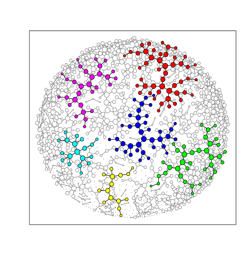
Figure 1: A network sample of 1200 people from a high-risk hidden population. Some sample components are highlighted. The network sample is resampled many times using a network sampling design that adheres closely to the original survey design. The frequency that a person is included in the resamples (circle diameter) is used to estimate the person’s inclusion probability in the original sample. These estimated inclusion probabilities enable estimates of hidden-population characteristics.

Network sample surveys are in wide use around the world for studies of hard-to-reach vulnerable populations [White et al. (2015), Verdery et al. (2015)]. In these surveys social links are followed from people already in the sample to find and bring new people into the sample. For the key populations at high risk for HIV these methods provide the most effective way to gain scientific understanding about the behavioral, biological, and network risks. These studies have been supported by the U.S. President’s Emergency Plan for AIDS Relief (PEPFAR) and the Centers for Disease Control and Prevention (CDC) and other national and international organizations, with research on the methodologies supported by the National Science Foundation and National Institutes of Health NIH [Mouw and Verdery (2012)]. The annual UNAIDS statistics on HIV depend in part on network surveys [UNAIDS (2018)]. The surveys are essential for basic scientific understanding, for assessing network risk even before any virus moves in, and for evaluating the effectiveness of intervention programs. Policy decisions in response to outbreaks of HIV and other emerging epidemics require accurate estimates from these network surveys.

The estimation methods currently used with the survey data are known to be inaccurate, with large mean squared errors and biases and unreliable confidence intervals [Goel and Salganik (2010), Gile and Handcock (2010)]. The inaccuracies arise because different people in the hidden population have different probabilities of coming into the sample. A person in a highly connected region of the population will have a higher inclusion probability than one in a less connected position. The adjustments currently made for these unequal inclusion probabilities are based on assumptions about the sampling design that are discrepant from the survey designs actually used. The estimators derived from the unrealistic assumptions do not use the full sample data available and in particular ignore the network topology of the sample.

New estimators introduced in this report remove almost all of the bias, have much lower mean squared errors, and enable confidence intervals having good coverage probabilities and modest widths. The improvements are achieved by using the full sample network data and incorporating the key features of the actual survey design. For the new estimates, a sampling process similar to the actual survey design is run on the sample network data. The frequency with which a person is included in the sampling process provides an estimate of that person’s inclusion probability in the actual survey. The estimated inclusion probabilities are then used in a generalized unequal probability estimator to estimate characteristics of the hidden population, such as proportion infected with a virus, prevalence of a risk behavior such as exchanging sex for money, mean number of partners per person, or rate of concurrent relationships.

In the actual network survey, the probability that a person is included depends on the person’s position in the social network topology in interaction with the type of sampling design used. The new method estimates the inclusion probabilities from the sample network topology in interaction with the same type of sampling design.

Figure 1 shows the network topology of a sample of 1200 people from a high-risk population of drug users, sex workers, clients and other partners. The nodes represent individuals (circles) and the lines represent sexual, drug, and social relationships between pairs of individuals. The sample network topology emerges as the connectedness pattern of the paths. The sample network topology includes separate sample components, several of which are highlighted. Within a component, the sample network topology has a tree structure. The tree structure is a result of the design protocol, in which a person is not allowed to be recruited more than once. The population network, from which the sample is selected, is not a tree but has a more general net-like topology and larger components than appear in the sample.

The sample of Figure 1 was selected by the most commonly used form of network sampling, Respondent-Driven-Sampling (RDS), in which an initial sample of seeds is selected by investigators and each person is given up to three coupons with which to recruit up to three of their partners into the sample. When a person with a coupon comes in to be interviewed, that recruit is in turn given three coupons which which to recruit additional sample members, and so on. An individual is not allowed to be recruited more than once, which results in the tree structure of the sample topology. The three-coupon limit restricts branching of the network sample to three. So counting the person who recruited the individual gives a maximum of four links from any individual in Figure 1. Not every coupon issued is used, and not every individual recruited comes in to be interviewed, although there is a monetary incentive offered to both the recruitee and the recruiter.

If unlimited branching is allowed, or if a high coupon limit such as 15 is used, the network design is typically referred to as Snowball (SB) sampling. Snowball samples tend to include some larger sample components. With either design, coupons are given an expiration date, such as 28 days from the date of issue. Recruitment in a sample component comes to an end if there are no links out from people in the sample with unexpired coupons to people not already in the sample.

Early uses of network sampling for hard-to-reach populations typically used Snowball Sampling methods, with survey data summarized by unweighted sample means and proportions [Spreen (1992), Heckathorn (1997), and Thompson and Collins (2002)]. Statistical estimates of population values from relatively simple network sampling designs were obtained by Birnbaum and Sirken (1965) and Frank (1977), Frank and Snijders (1994).

Starting with Heckathorn (1997), the methodology of Respondent-Driven-Sampling using dual-incentive coupons was introduced. Estimators for these designs based on random walk theory and assumptions of Markov transitions in the sampling between values of attribute variables of respondents were given in Salganik and Heckathorn (2004), Heckathorn (2007), and Volz and Heckathorn (2008). If a random walk with replacement is run in a network consisting of a single connected component, the long term frequency of inclusion of node $i$ is proportional to $d_{i}$. One consequence of the use of random-walk theory to justify the estimators was that the more freely branching snowball designs became more seldomly used, with the idea that the designs restricting branching to 3 or fewer links would be closer to the assumed random walk model.

The estimator of Volz and Heckathorn (2008) (VH estimator), uses $d_{i}$ in place of actual inclusion probability in an unequal probability estimator. The estimator of Salganik and Heckathorn (2004) (SH estimator) used the same form as VH to estimate mean degree, and for means of binary attribute variables adjusts that with proportions of sample recruitment links between and within the group with the attribute and the group without it. The adjustment is based on the additional assumption of Markov transitions between attribute states during the sampling. Adjustments for surveys in which sample size is a large fraction of population size include the Successive Sampling (SS) estimator Gile (2011) for the VH estimator and the Homophily Configuration Graph (HCG) estimator Fellows (2018) for the SH estimator.

A random walk design in a network at each step allows tracing of only one randomly selected link from the current node (person), and sampling is done with replacement so the same person can be selected again later. The inaccuracies of the widely-used current estimators result from the discrepancy between the assumed random walk model, which has no branching and is with-replacement, and the designs actually used in the surveys, with their branching and without-replacement sampling. Additionally, the current estimators use an assumption that the population network has only a single component, in support of the theoretical properties of the random walk model. Evidence suggests that many real population include more than one connected components. An additional assumption underlying some of the current approaches to estimation assumes first-order Markov chain transitions during the sampling between attribute values of selected nodes. The types of networks that would support this assumption are unlikely to be encountered with real network populations [Verdery et al. (2015)].

Currently used estimators such as the VH and related estimators do not make use of the sample network topology of the data. Instead, they use the number of partners (degree) reported by each individual. The SH and related estimators use, in addition to degree, counts of sample links between groups having different values of an attribute, but not the pattern of network paths by which the links connect together.

Confidence interval methods proposed for RDS designs have most often been based on bootstrap methods [ Salganik (2006), Gile (2011)]. Evaluations of these methods with various real and simulated network populations include Spiller et al. (2017) and Baraff, McCormick and Raftery (2016).

The concern of the work above and of the present report is estimation of population characteristics, such as prevalence of infection, proportion of people with a risk-related behavior, mean degree, or concurrency. The related problem of estimating the size of a hidden population with network sampling is addressed in Handcock, Gile and Mar (2014), Crawford (2016), Crawford, Wu and Heimer (2018), and Vincent and Thompson (2017). Another closely related problem is use of network designs to adaptively spread interventions in a population [Valente (2012)]. In fact network sampling for at-risk populations as described in this report whose primary purpose is fundamental knowledge and estimation usually bring beneficial interventions as well to the hard-to-reach population. Such interventions include testing for HIV and other infections, referral to medical services and enhanced adherence counselling for individuals who test positive, referral to addiction treatment programs, and distribution of condoms or clean injection equipment. Link-tracing designs have been shown to be a highly effective way to introduce and distribute interventions in a population [Thompson (2017)].

An RDS design to study a rural opioid user network in relation to HIV risk was used in Young, Rudolph and Havens (2018), Young et al. (2014), and Young et al. (2013). The project used an additional design feature of a social network study of sample members which enabled examination of differential recruitment rates for partners having different attribute values.

For the new estimation approach described here we make no assumption of any form or model for the population network. Instead we use the sample network and its topology just as it is in the data. Instead of any unrealistic assumption about the sampling design, we use the same type of design as used in the actual survey, and use it to select many re-samples of the sample network. The actual survey design for a survey is documented in the survey protocol document and survey reports. Typically it allows branching up to the coupon limit and is done without replacement.

The theory used for the new estimation method is the design-based theory of inference in sampling [Särndal et al. (1978)], in which the population—here including its network—is conceived as fixed but unknown and inference is done using the design-induced probabilities by which the sample was selected. The key to the new method is to use the full sample network to estimate the probability with which each person was included in the sample. These inclusion probabilities can no be known exactly, because they depend on the population network topology both inside the sample and outside it.

The idea of the new method is very simple (first described in the technical papers Thompson (2018) and Thompson (2019)). We run a sampling process similar to the actual survey design on the sample network data and use the inclusion frequencies in the sampling process to estimate the inclusion probabilities in the real-world sampling. With the estimated inclusion probabilities, well-established sampling inference methods can be used for population estimates and confidence intervals. Details of the re-sampling and estimation are described in the Supplement. Two approaches to the re-sampling are repeated re-samples and a Markov chain resampling process. For the simulations we use the resampling process because it is computationally so fast.

The size of a node in Figure 1 is drawn with diameter proportional to the inclusion frequency of that person in the re-sampling process. A node in a more central position in a component has a higher inclusion frequency than one is a more peripheral position in the sample network topology. Nodes in larger components also tend to have higher inclusion frequencies because more network paths lead to them. If we look at nodes with just one link in Figure 1, they vary in size one to another, with those connected to a more central part of the component having higher inclusion frequency. A similar variation in size can be seen among nodes with two links, and so on. So inclusion frequency is not a simple function of node degree but depends on position in the network topology. Note that the relevant centrality measured here by node diameter is not a calculation from the network topology alone but with the interaction of that topology with the branching network sampling design.

2 Methods

The new estimation method

In traditional survey sampling with unequal probabilities of inclusion for different people, typical estimators divide an observed value $y_{i}$ for the $i$th person by the inclusion probability $\pi_{i}$ that person. A variable of interest $y_{i}$ can be binary, for example 1 if the person tests positive for a virus and 0 otherwise, or can be more generally quantitative, such as viral load. The inverse-weighting gives an unbiased or low-bias estimate of the population proportion or mean of that variable. In network surveys the inclusion probabilities are unknown so they need to be estimated.

The estimators described in this report first estimate the inclusion probability of each person in the sample by selecting many resamples from the network sample data using a design that adheres in key features to the actual survey design used to find the sample. In particular, the resampling design is a link-tracing design done without-replacement and with branching, as was the original design. The frequency $f_{i}$ with which an individual is included in the resamples is used as an estimate of that person’s inclusion probability $\pi_{i}$.

What we do is select $T$ resamples $S_{1},S_{2},...,S_{T}$ from the sample network data. There are two approaches to selecting the sequence of resamples. In the repeated-samples approach each resample is selected independently from seeds and progresses step-by-step to target resample size independently of every other resample, so we get a collection of independent resamples. in the sampling-process approach each resample $S_{t}$ is selected from the resample $S_{t-1}$ just before it by randomly tracing a few links out and randomly removing a few nodes from the previous resample and using a small rate of re-seeding so we do not get locked out of any component by chance. It is this Markov resampling process approach that we use for the simulations in this paper because it is so computationally efficient.

For an individual $i$ in the original sample, there is a sequence of zeros and ones $Z_{i1},Z_{i2},...,Z_{iT}$, where $Z_{t}$ is 1 if that person is included in resample $S_{t}$ and is 0 if the person is not included in that resample. The inclusion frequency for person $i$ is

$$f_{i}=\frac{1}{T}\left(Z_{i1}+Z_{i2}+...+Z_{iT}\right)$$ (1)

In Figure 1 the circle representing individual $i$ in the sample is drawn with diameter proportional to the estimated inclusion probability $f_{i}$ of that individual. Individuals centrally located in sample components tend to have high values of $f_{i}$. That is because there are more paths, and paths of higher probability, leading the sample to those individuals. Also, individuals in larger components tend to have larger $f_{i}$ than individuals in smaller components, so that the method is estimating inclusion probability of an individual relative to all other sample units, not just those in the same component or local area or the sample This is because of the self-allocation of the branching design, even in the absence of re-seeding, to areas of the social network having more links and connected paths.

The estimator of the mean of a characteristic $y$ in the hidden population is then

$$\hat{\mu}_{f}=\frac{\sum(y_{i}/f_{i})}{\sum(1/f_{i})}$$ (2)

where each sum is over all the people in the sample. If the actual inclusion probabilities $\pi_{i}$ were known and replaced the $f_{i}$ in Equation 2 we would have the generalized unequal probability estimator $\hat{\mu}_{\pi}$ of Brewer Brewer (1963).

Why it works

To understand why the new method works, consider the two stages of sampling. The first-stage is the actual network sampling design by which the sample of people is selected from the hidden population. The second-stage design selects a resample of people from the network sample data, using a network sampling design similar to the one used in the real-world. The second-stage design, like the first, uses link-tracing, branches, and is done without-replacement. The second-stage design can not be exactly the same as the original design in every respect. For example the second-stage design has to use a smaller sample size than the original, because of the without-replacement sampling.

The probability that individual $i$ in the original sample is included in the resample will be called $\phi_{i}$. The ideal is to have the inclusion probability for a unit at the second stage, given the first stage sample, to be proportional to it’s inclusion probability in the original design. That is, $\phi_{i}=c\pi_{i}$, where $c$ is some constant, which does not need to be known.

Now let $\hat{\mu}_{\phi}$ be formula 2 with the exact resample probabilities $\phi_{i}$ replacing $f_{i}$. If $\phi_{i}=c\pi_{i}$, then $\hat{\mu}_{\phi}=\hat{\mu}_{\pi}$, because the constant of proportionality $c$ is in both the numerator and denominator of 2 and divides out of the estimator.

As the number of resamples $T$ gets large the inclusion frequencies $f_{i}$ converge in probability to the second-stage inclusion probabilities $\phi_{i}$. This is by the (weak) Law of Large Numbers for the independent resamples and by the Law of Large Numbers for Markov chains for the resampling process that traces a few and removes a few at each step.

It follows that if $\phi_{i}$ is proportional to $\pi_{i}$ then $\hat{\mu}_{f}$ converges in probability to $\hat{\mu}_{\phi}$. So if inclusion in the resample $\phi$ is proportional to inclusion in the original sample $\pi$ then the estimator we use here $\hat{\mu}_{f}$ converges to the general unequal probability estimator $\hat{\mu}_{\pi}$. Since the resampling is fast computationally, especially with the sampling process approach, we can readily select a lot of resamples, such as $T=10,000$ that we use in the simulations here, and higher values of $T$ like one million are still fast to compute.

The approximate part is in how close the second-stage inclusion probabilities $\phi_{i}$ are to proportionality with the first-stage inclusion probabilities $\phi_{i}$. This is why it is important that the resampling design adheres to the main features of the actual network design, such as network link tracing, branching, and without-replacement selections.

The use of the second stage sample is different here than in traditional two-stage sampling or in bootstrap methods. In each of those a given second-stage sample is used to make an estimate of a population value. In the case of bootstrap methods, many such estimates, from the many resamples, are used to construct a confidence interval. If the sampling is with unequal probabilities at each stage, estimation of the population value from the second-stage sample requires dividing first by the second-stage inclusion probability $\phi_{i}$ to estimate what is in the first stage sample and then then by the first stage probability $\pi_{i}$. Here we use the second stage design solely to estimate its own inclusion probabilities and we construct the second-stage design to have those probabilities similar to the first-stage probabilities.

Confidence intervals

When an estimator has a large bias, it is hard to have a confidence interval with adequate coverage probability based on that type of estimator. Such an interval has to be extra wide to accommodate not only the sampling variance but the offset between the expected value of the estimator and the true population value. This is why confidence intervals for the current estimators have been problematical. The confidence interval here takes advantage of the better estimate we get by using the resampling process inclusion frequencies $fi$ to estimate the actual inclusion probabilities. The confidence interval method for the new estimators uses the $fi$ again in forming the interval, using unequal probability sampling methods.

A simple variance estimator to go with $\hat{\mu}_{f}$ is

$$\widehat{\textrm{v}ar}(\hat{\mu})=\frac{1}{n(n-1)}\sum_{s}\left(\frac{ny_{i}/f_{i}}{\sum_{s}(1/f_{i})}-\hat{\mu}_{f}\right)^{2}$$ (3)

This is based on a variance estimator from unequal probability sampling but is modified here to serve the generalized unequal probability estimator and uses the inclusion frequencies $f_{i}$ in place of the unknown actual inclusion probabilities. An approximate $1-\alpha$ confidence interval is then calculated as $\hat{\mu}\pm z\sqrt{\widehat{\textrm{v}ar}(\hat{\mu})}$, with $z$ the $1-\alpha/2$ quantile from the standard Normal distribution. In the simulations here the estimator above gives a slightly higher average confidence interval coverage probability.

3 Results

The new estimators are evaluated and compared with the current estimates using the network data on the hidden population at risk for HIV enumerated in the Colorado Springs study on the heteroxexual transmission of HIV [Potterat, Rothenberg and Muth (1999)], also known as the Project 90 study. The study was so thorough in finding every linked person that it provides the most relevant network data set that can be considered as an entire at-risk population for the purpose of comparing sampling designs and estimators. The population and the simulation methods are described in more detail in the Methods section.

The most commonly used estimator with network surveys in current practice is the VH estimator. The other variations in use such as SH are related to it and are based on the same assummptions plus the additional assuption of a first-order Markov process in transitions between node attribute values during the sampling. The SH estimator is used mainly for binary attribute variables. For categorical variables it has the property that the proportion estimates do not add to one without extra adjusting of one kind or another, and it is not well suited to continuous variables. Goel and Salganik (2010) found that the SH estimator performed about the same as the VH estimator, and Gile and Handcock (2010) found SH performed a little less well than the VH estimator. For all of these reasons we use the VH estimator as the basis of comparisons with the new estimator in this section.

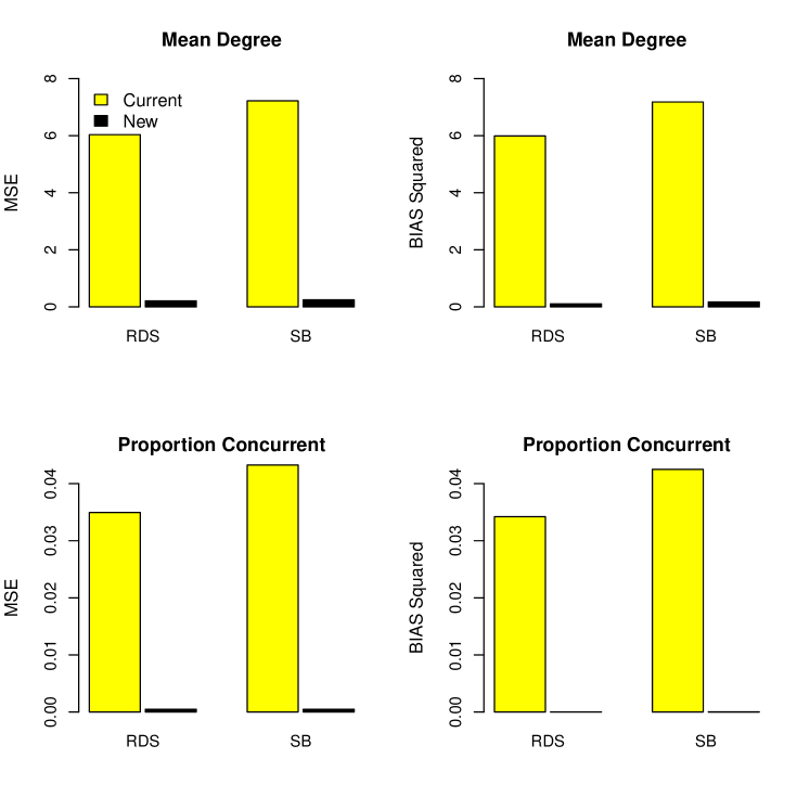
Figure 2: The mean square error (left) and bias (right) of the new estimator (black) is lower than that of the current estimator (yellow) for estimating mean degree (top) and concurrency—proportion of people with two or more partners (bottom) for each network sampling design. The design RDS restricts branching by limiting coupons to a maximum of 3. The snowball (SB) design gives respondents as many coupons as their number of partners, up to a maximum of 15, allowing almost unlimited branching as the sample is selected.

Link-related variables

Among the most important quantities to estimate in relation to spread of HIV are the means and proportions of link-related variables. Two of widespread interest are mean degree) and concurrency. Mean degree is the average number of partners per person in the population. The most common definition oncurrency is the proportion of people in the population who have two or more partners. This and related definitions of concurrency and their role in spreading HIV are discussed in Kretzschmar and Morris (1996), Morris and Kretzschmar (1997), and Admiraal et al. (2016). A high number for either of these is an indication that an epidemic could spread rapidly in the population once it starts there.

The top two plots in Figure 2 are on estimating mean degree. Plots on the left show MSE. Plots on the right show squared bias. The top row is for the RDS design with 3 coupons. The bottom row is for the SB design with 15 coupons. The current estimator (VH) is shown in yellow and the new estimator in black. For any estimator, the MSE equals the variance plus the bias squared. MSE and bias squared are plotted on the same scale, so it is easy to see that most of the reduction of bias with the new estimator comes by reducing, almost eliminating, the bias.

Starting with the left-most pair of bars, the mean square error for the current method for RDS sampling is 6.03. The mean square error for the new estimator is 0.21. The reduction in mean squared error comes largely from eliminating most of the bias, as shown in the top right plot of Figure 2. The actual mean degree in the Colorado Springs study population is 7.89 partners per person. The current estimator underestimates this on average by 2.45 partners. The new estimator overestimates by only 0.32 on average.

Here the squared bias 5.99 accounts for almost all of the MSE 6.03. The new estimator reduces the squared bias to 0.11. The reduction in bias is obtained by the more accurate estimates of inclusion probabilities using a the resampling design that adheres to the the branching and without-replacement features of the actual survey design, and using the sample network recruitment data instead of assumptions about the hidden population network.

For estimating mean degree, with either the RDS or the SB design the relative efficiency (ratio of MSEs) of the new estimator is 29. So with the same design, the new estimator reduces the mean squared error to 1/29 that of the current method. For estimating the proportion of people in the population with two or more partners (concurrency, bottom row in Figure 2), the relative efficiencies of the new estimators compared to the current estimators are 72 for RDS and 92 for the SB design.

The reason for the dramatic improvement of the new estimates over the current estimates for the link-related quantities is that a link-related variable such as number of partners or having two or more partners is strongly related to the actual inclusion probabilities of the link-tracing design, whether the design is RDS or SB. Therefore with these variables it helps very much to have accurate estimates of the inclusion probabilities, and large deviations from those probabilities result in poor estimator performancce.

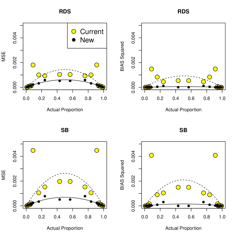
Figure 3: Mean squared error of the estimate of population proportion for each of 13 individual attributes. The new estimator (black) is compared to the current estimator (yellow). To help see the pattern, the estimate of the compliment of each attribute is shown. The compliment of sex work client, for example, is not-client. A parabolic curve is fitted by weighted least squares to the MSEs of the new estimator (solid line) and the current estimator (dashed line). The new estimator MSEs have a lower fitted curve with a better fit with each design.

Node attribute variables

The Colorado Springs Study node data includes 13 individual attribute variables such as sex worker, client of sex worker, or unemployed. These are variables 2 through 14 in Table 1. For an individual, the value is 1 if the individual has the attribute and 0 otherwise. The object for inference for each attribute is to estimate the proportion of people in the population having that attribute. Most of these variables, such as sex or race or employment status, are not strongly or consistently related to inclusion probabilities. Still, for design-based estimators to work well it helps to have the estimated inclusion probabilities close to the actual inclusion probabilities. For the simulations, missing values were arbitrarily set to zero so that sample sizes would be the same for all variables.

With a conventional simple random sampling design for estimating a population proportion, the mean squared error of the estimate is a parabola-shaped function of the actual population proportion. The actual proportion has to be between zero and one. The MSE is highest when the actual proportion is one-half and the MSE is zero when the actual proportion is zero or one. With the network designs and their unequal inclusion probabilities the situation is more complex, but it is still the case that the actual proportion has to be between zero and one and that the MSE will be zero if the actual proportion is zero or one.

To help see the pattern in the mean squared errors for estimating the population proportions of the 13 attribute variables, the MSE for each variable is plotted in Figure 3 against the actual proportion of people having that attribute in the Colorado Springs study population. For each of the 13 variables, we can also estimate the proportion for its complement. The compliment of “client”, for example, is “not client”. The proportion for the compliment is 1 minus the proportion with the attribute, and the MSE for estimation the compliment is the same as the the MSE for estimation of the original variable. This gives us 28 variables for each plot in Figure 3, with actual proportions ranging from near 0 to near 1. The original variables are on the left, since the actual proportions are all less than one-half. The compliment variables provide redundant information but clarify the pattern in the MSEs.

The MSE with the new estimator (black in plots) is lower than that of the current estimator in all cases except for some of the ones with actual proportion near to zero for which the MSE is very small with either estimator. While the MSEs of the new estimator fall rather close to the fitted parabola (solid line), the MSEs of the current estimator are more erratic and the fitted parabola (solid line) is higher. The overall higher MSEs and erratic pattern with the current estimator result from the discrepancies between actual inclusion probabilities and those used in estimation.

The parabolas in the plots have form ${\rm MSE}=ap(1-p)$ where $p$ is the actual proportion, which is known for each of the 13 attribute variables in the simulation population. The coefficient $a$ measures the height of the fitted parabola for a given estimator-design combination. Since the relationship is linear with increasing variance in the quantity $p(1-p)$, the weighted least squares regression estimator of the coefficient $a$ is a simple ratio estimator. The parabola height provides a useful summary of the overall performance of the estimator-design combination. Because of the simple nature of a ratio estimate, the ratio of height coefficients of two estimator-design combinations is simply the the average MSE for the one combination divided by average MSE for the other combination.

For instance with the design RDS, the parabola for the current estimator (dashed line in Figure 3) is 2.4 times as high as the parabola for the new estimator. Equivalently, because of the simple nature of the ratio estimator, the average MSE for the 13 attribute variables with the current estimator is 2.4 times the average MSE with the new estimators. So the overall relative efficiency of the new estimator is 2.4. With the SB design, the overall relative efficiency of the new estimator is 3.8. So we get a substantial gain in efficiency with the new estimators even for variables that, unlike the link-related variables, do not have an obviously strong or consistent relationship with the network sampling inclusion probabilities. The plots indicate that again much of this gain from from a big reduction of bias with the new estimators.

Confidence interval coverage probabilities for each variable for each of the 15 variables are given in the Supplemental Tables. While the nominal coverage is 95 percent, the actual coverage probability is assessed in the simulation as the proportion of the 1000 runs, corresponding to 1000 original samples of size 1200 each, for which the sample confidence interval contained the true value for the population. For the values rounded to 1.0 in the last row of the table, the exact coverage proportions were 0.999 and 0.998. The median coverage probability of the intervals for the 15 characteristics estimated with each of two designs is .94.

4 Discussion

The new estimators obtain better estimates of key population characteristics from network survey data because the method uses the full network topology of the data in interaction with the type of sampling design actually used, which includes branching and without-replacement sampling. This is in contrast to currently used estimators which derive estimates from unrealistic assumptions about the design and the population network. Because of the strategic importance of network surveys for understanding and reducing the HIV pandemic and emerging epidemics, it is highly desirable and urgent to bring the new estimators into practice.

The advantage of the new estimators is especially great for estimating link-related quantities such as mean degree and concurrency, for which the values are strongly related to survey inclusion probabilities. The link-related variables are directly related to the network risk of HIV spread in the population. The elimination of most of the bias through the new estimation method enables confidence intervals of modest width to have coverage probabilities close to the desired nominal value.

The new methods work for the freely branching network designs such as snowball sampling as well as for the limited-branching designs such as the RDS designs as currently practiced. The current estimators perform poorly for the freely branching designs because those designs are the most far from the assumed random walk. Computationally the calculations of the new estimators are fast and scale up well because of the use of a sampling process approach that stays close to the desired equilibrium distribution.

The new estimation approach should work also for a wide range of network related sampling designs and applications. Because the new estimation method scales up well, these include studies of online social network communities and their characteristics and other large network estimation problems [Papagelis, Das and Koudas (2011), Gabielkov, Rao and Legout (2014)]. Another type of network design in which the new estimators could contribute involves contact tracing for intervention in outbreaks of sexually transmitted diseases. In these network designs only contacts of people who test positive are traced and then tested and treated in necessary. Peters et al. (2016) and Campbell et al. (2017) report on a study in which contract tracing was used after an HIV outbreak associated with opioid misuse in Indiana had spread rapidly. The traced network together with phylogenetic data from sequencing of virus strains was used to determine where the outbreak started and how it spread. Because the contact tracing procedure is another network sampling design variation, it is possible that the estimators introduced here could contribute to such network analyses. Adaptive spatial designs used for monitoring surveys of rare and endangered plants and animals can be recast as network sampling problems (Thompson (2006), Thompson (2011)). Once in that framework, the inference methods proposed here apply immediately.

One finding that emerges from this study is that the network survey designs as currently used are good and provide invaluable information. Increased accuracy of estimates from these designs will increase the value of the data collected. The designs are highly effective at reaching into the key areas of hard-to-reach populations. Researchers can feel free to use a wider range of designs, such as those that more freely branch, as suits each particular situation. The new estimates work well with each of these design variations. The findings from these surveys are needed for effective interventions and policy to alleviate critical problems for vulnerable populations. The work of policy makers involved with programs concerned with vulnerable populations will benefit from the increased value of the survey network data.

Supplement to New estimates for network sampling

Introduction to supplement

The Supplement includes Details on methods, Supplemental Tables. The Methods details section includes additional explanation of the new estimation method for network surveys and why it works; additional description of the two approaches, repeated samples and sampling process, to calculating the inclusion frequencies $f_{i}$ which estimate the real-world inclusion probabilities $p_{i}$; description of the simulations; additional details and variations on the estimators and variance estimators; and location of the data and the source C code for the sampling process algorithm for estimating the inclusion probabilities. The Supplemental Tables include the numbers behind the figures and additional values such as expected values of the variances of estimators and mean confidence interval half-widths.

Details on methods

Repeated samples and sampling process

The inclusion frequencies $f_{i}$ are calculated by re-sampling the sample network many times using a design similar to the original design used to select the members of the hidden population from the real world. Two approaches to the resampling are to repeatedly select independent resamples, each from seeds to target sample size, and to select the sequences of resamples using a Markov-chain resampling process.

In the simulations of the paper only the sampling process approach was used. The repeated-sample approach is illustrated here first as understanding that makes the sampling-process approach easier to understand.

Figure 1 of the text shows an RDS sample of 1200 people selected from the Colorado Springs network population of sex workers, drug users, and partners of each (Potterat, Rothenberg and Muth (1999)). The target sample size of the resamples is 400.

The simulation study selected 1000 samples of 1200 from the population, for each of the two designs RDS and SB. The simulation study used the sampling process method, which is computationally very much faster than the independently repeated samples.

Given the network sample obtained from the real world network sampling design, we obtain a sequence of re-samples

$$\{S_{1},S_{2},S_{3},...,S_{T}\}$$

from the network data using a fast-sampling process similar to the original design. $T$ is the number of iterations.

For unit $i\in U_{s}$, there is a sequence of indicator random variables:

$$\{Z_{i1},Z_{i2},Z_{i3},...,Z_{iT}\}$$

where $Z_{it}=1$ if $i\in S_{t}$ and $Z_{it}=0$ if $i\notin S_{t}$, for $t=1,2,...,T$, the number of iterations of the sampling process.

The average

$$f_{i}=\frac{1}{T}\sum_{i=1}^{T}Z_{i}$$

is used as an estimate of the relative inclusion probability of unit $i$ in the similar design used to obtain the data from the real world. If the real-world network design is done without replacement, then the fast-sampling process is also carried out without replacement.

In the repeated-sample approach, each sample in the sequence proceeds from selection of seeds to target sample size. With this approach the samples in the sequence $\{S_{1},S_{2},S_{3},...,S_{T}\}$ are independent of each other.

In the sampling-process approach, each sample $S_{t}$ is selected dependent on the one before it, $S_{t-1}$. To get from $S_{t}$ to $S_{t-1}$ we probabilistically trace links out from $S_{t}$, randomly drop some nodes from $S_{t}$, and may with low probability select one or more new seeds. Advantages of the sampling-process approach are first, that the computation can be made very fast. Second, the sampling process is fast-mixing and once it reaches it’s stationary distribution every subsequent sample $S_{t}$ is in that distribution. The stationary distribution of the sequence of samples represents a balance between the re-seeding distribution, which can be kept small with a low rate of re-seeding, and the design tendencies arising from the link-tracing and the without-replacement nature of the selections.

The sampling process is without-replacement in that a node in the sample can not be selected again while it is in the sample. Once it has been removed from the sample it can be selected anew at any time. With the sampling-process design, the sequence of fast samples $S_{1},S_{2},...$ forms a Markov chain of sets, with the probability of set $S_{t}$ depending only on the previous set $S_{t-1}$.

In the simulations the repeated-sample design selects initial seeds using Bernoulli sampling. A low rate of re-seeding is used, mainly to ensure that the growth of the sample can not get stuck before target sample size is reached. A medium rate of link-tracing is used. Links out are traced with independent Bernoulli selections. Because no coupons were used in the re-sampling, each selected node can continue to recruit without time limit.

The sampling process can use a high tracing rate because removals offset the tracing to maintain a stochastic balance around target sample size. A relatively high rate of ongoing reseeding rate is used so that the process does not get locked out of any components. Whenever the sample goes above target sample size, the sample is randomly thinned with removals, with probability of removal set to make expected sample size back within target at the next step. All these features make the process very fast mixing.

Specifically, in the examples we trace the links out from the current sample $S_{t}$ independently, each with probability $p$. Nodes are removed from the sample independently with probability $q$. The removal probability $q$ is set adaptively to be $q_{t}=(n_{t}-n_{\rm target}/n_{t}$ if $n_{t}>n_{\rm target}$ and $q_{t}=0$ otherwise, so that sample size fluctuates around its target during iterations. Sampling is without replacement in that a node in $S_{t}$ is not while it remains in fast sample, but it may be reselected at any time after it is removed from the fast sample. The re-seeding rate can be low because the seeds at the beginning of each sample serve to get the sample into enough components.

In the repeated-samples design, the seeding rate $p_{s}=0.0167$; the tracing rate is $p=0.05$, and the re-seeding rate is $p_{r}=0.001$. The sampling-process design uses no initial seeds, relying on the re-seeding to initialize the process and bring it quickly into its stationary distribution. The removal rate $q$ is set adaptively as described above to keep the process in fluctuation around its target sample size. The re-seeding rate is $p_{r}=0.01$. Even though the re-seeding rate is relatively high, at each step most added nodes are added by tracing links, because that rate is so much higher. The re-seeding serves to keep the process from getting permanently locked out of any component through removals.

If the real-world survey sampling is done with replacement, one can use a re-sampling design that is with replacement. An advantage of this is that a target sample size for the fast design can be used that equals the actual sample size used in obtaining the data. However, in most cases the real design is done without replacement.

Sampling processes of these types are discussed in (26) Thompson (2017) for their potential uses as measures of network exposure of a node, or a measure of network centrality, or a predictive indicator of regions of a network where an epidemic might next explode. Calculation of the statistic $f_{i}$ for each unit in the network sample can be used as an index of the network exposure of that unit. A high value of $f_{i}$ indicates the unit has high likelihood of being reached by a network sample such as ours. It will also have a relatively high likelihood of being reached by a virus, such as HIV, that spreads on the same type of links by a link-tracing process that is broadly similar. A given risk behavior will be more risky for a person with high network exposure. For a person in a less well connected part of the network, the same behavior carries lower risk. Since a purpose of the surveys is to identify risk characteristics, an index of network exposure measures another dimension of that risk, beyond the individual behavior and health measures. Here, however, are interested in their usefulness for estimating population characteristics based on link-tracing network sampling designs.

Estimators

This supplemental section contains additional detail on estimation formulas. It includes estimation when the original design is carried out with replacement and estimation of a ratio.

Network sampling designs select units with unequal probabilities. With unequal probability sampling designs, sample means and sample proportions do not provide unbiased estimates of their corresponding population means and proportions.

To estimate the mean of variable $y$ with an unequal-probability sampling design, the generalized unequal probability estimator has the form

$$\hat{\mu}_{\pi}=\frac{\sum_{s}(y_{i}/\pi_{i})}{\sum_{s}(1/\pi_{i})}$$ (4)

where $\pi_{i}$ is inclusion probability of unit $i$.

With the network sampling designs of interest here, the inclusion probabilities $pi_{i}$ are not known and can not be calculated from the sample data. To circumvent this problem the Volz-Heckathorn Estimator uses degree, or self-reported number of partners, to approximate inclusion probability:

$$\hat{\mu}_{d}=\frac{\sum_{s}(y_{i}/d_{i})}{\sum_{s}(1/d_{i})}$$ (5)

in which $d_{i}$ is the degree, the number of self-reported partners, of person $i$.

The rationale for this approximation is that if the sampling design is a random walk with replacement, or several independent random walks with replacement and the population network is connected, then the selection probabilities of the random walk design will converge over time to be proportional to the $d_{i}$. Here connected means that each node in the population can be reached from any other node by some path, or chain of links, so that the population network consists of only one connected component. Biases in this estimator result from the use of without-replacement sampling in the real-world designs, the use of coupon numbers $k$ greater than 1 making the design different from a random walk, population networks being not connected into a single component, or slow mixing due to specifics of the population network structure.

The new estimator, with a non-replacement sampling design, is

$$\hat{\mu}_{f}=\frac{\sum_{i\in s}(y_{i}/f_{i})}{\sum_{i\in s}(1/f_{i})}$$ (6)

where $f_{i}$ is the inclusion frequency of unit $i$ in the resampling process run on the sample network data.

A simple variance estimator to go with the new estimator is

$$\widehat{\textrm{v}ar}(\hat{\mu}_{f})=\frac{1}{(\sum_{i\in s}1/f_{i})^{2}}\sum_{i\in s}\frac{(y_{i}-\hat{\mu}_{f})^{2}}{f_{i}^{2}}$$ (7)

Another simple variance estimator is

$$\widehat{\textrm{v}ar}(\hat{\mu})=\frac{1}{n(n-1)}\sum_{s}\left(\frac{ny_{i}/f_{i}}{\sum_{s}(1/f_{i})}-\hat{\mu}_{f}\right)^{2}$$ (8)

An approximate $1-\alpha$ confidence interval is then calculated as

$$\hat{\mu}_{f}\pm z\sqrt{\widehat{\textrm{v}ar}(\hat{\mu}_{f})}$$ (9)

with $z$ the $1-\alpha/2$ quantile from the standard Normal distribution.

The variance estimator 7 is based on, and simplified from, the Taylor series linear approximation theory for generalized unequal probability estimator. Linearization leads to the estimator of the variance of the generalized estimator

$$\widehat{\textrm{v}ar}(\hat{\mu}_{\pi})=\frac{1}{(\sum_{i\in s}1/\pi_{i})^{2}}\sum_{i\in s}\sum_{j\in s}\check{\Delta}_{ij}\frac{(y_{i}-\hat{\mu}_{\pi})}{\pi_{i}}\frac{(y_{j}-\hat{\mu}_{\pi})}{\pi_{j}}$$ (10)

where

$$\check{\Delta}_{ij}=\frac{\pi_{ij}-\pi_{i}\pi_{j}}{\pi_{ij}}$$

where $\pi_{ij}$ is the joint inclusion probability for units $i$ and $j$. A good discussion of the approach is found in Särndal, Swensson and Wretman (2003), with this variance estimator on p. 178 of that work. That type of variance estimator goes back to at least to Brewer and Hanif (1983) and is described on p. 178 in Särndal, Swensson and Wretman (2003). Here though it has been modified, first to apply to the generalized unequal probability estimatore instead of the Horvitz-Thompson estimator, and second by using the inclusion frequencies $f_{i}$ to estimate the inclusion probabilities $\pi_{i}$.

The variance estimator 8 is based on the idea that if the sum $\hat{\mu}_{f}=\sum_{i\in s}(y_{i}/f_{i})/\sum(1/f_{i})$ estimates $\mu$ then each piece $(y_{i}/f_{i})/\sum(1/f_{i})$ estimates $\mu/n$ and so $t_{i}=n(y_{i}/f_{i})/\sum(1/f_{i})$ would be an estimate of $\mu$, for $i=1,...,n$. Ignoring the dependence from the without-replacement sampling and treating $t_{1},...,t_{n}$ as uncorrelated, then $\hat{\mu}_{f}$ is the sample mean of the $t_{i}$ and 8 is their sample variance divided by sample size.

In simulations both 7 and 8 give decent variance estimates and confidence intervals. The coverage probability tended to be modestly better with 8, and that is the one used in the simulations of the report.

Consider an estimator of the variance using the full variance expression with the fast-sample frequencies $f_{i}$ in place of the $\pi_{i}$ and, in place of the joint inclusion probability $\pi_{ij}$, the frequency $f_{ij}$ of inclusion of inclusion of both units $i$ and $j$ in the fast sampling process. This would give

$$\widehat{\textrm{v}ar}(\hat{\mu}_{f})=\frac{1}{(\sum_{i\in s}1/f_{i})^{2}}\sum_{i\in s}\sum_{j\in s}\hat{\Delta}_{ij}\frac{(y_{i}-\hat{\mu}_{f})}{f_{i}}\frac{(y_{j}-\hat{\mu}_{f})}{f_{j}}$$ (11)

where

$$\hat{\Delta}_{ij}=\frac{f_{ij}-f_{i}f_{j}}{f_{ij}}$$

The double sum in the variance estimate expression will have $n(n-1)/2$ terms in which $i\neq j$. The most influential of these terms are the ones in which the joint frequency of inclusion $f_{ij}$ is relatively large. Because of the link tracing in the fast sampling process, sample unit pairs with a direct link between them will tend occur together more frequently than those without a direct link. An estimator using only those pairs with known links between them in the sample data would be

$$\widehat{\textrm{v}ar}(\hat{\mu}_{f})=\frac{1}{(\sum_{i\in s}1/f_{i})^{2}}\left(\sum_{i\in U_{s}}(f_{i}-1)\frac{(y_{i}-\hat{\mu}_{f})^{2}}{f_{i}}+\sum_{(i,j)\in E_{s}}\hat{\Delta}_{ij}\frac{(y_{i}-\hat{\mu}_{f})}{f_{i}}\frac{(y_{j}-\hat{\mu})}{f_{j}}\right)$$ (12)

where $E_{s}$ is the sample edge set. That is, $E_{s}$ consists of the known edges $(i,j)$ between pairs of units in the sample data. In general the size of the sample edge set $E_{s}$ will be much smaller that the $n^{2}$ possible sample node pairings $(i,j)$, or the $n(n-1)/2$ pairings with $i\neq j$, where $n$ is the sample size.

A further simplification and approximation for estimating the variance of the estimator is to use only the diagonal terms, that is,

$$\widehat{\textrm{v}ar}(\hat{\mu}_{f})=\frac{1}{(\sum_{i\in s}1/f_{i})^{2}}\sum_{i\in s}(1-f_{i})\frac{(y_{i}-\hat{\mu}_{f})^{2}}{f_{i}}$$ (13)

Dropping the coefficients $(1-f_{i})$, each of which is less than or equal to one, gives an estimate of variance that is larger, leading to wider, more conservative confidence intervals.

If the real-world network sampling design and correspondingly the re-sampling process are with-replacement, the estimator of $\mu$ is

$$\hat{\mu}_{f}=\frac{\sum_{i\in s}(m_{i}y_{i}/g_{i})}{\sum_{i\in s}(m_{i}/g_{i})}$$ (14)

in which $m_{i}$ is the number of times unit i is selected in the real design and $g_{i}$ is the average number of selection counts of unit $i$ in the fast sampling process.

If the real-world sampling design is with replacement, the re-sampling process can be done with replacement. In that case let $m_{t}(i)$ be the number of times node $i$ is selected at iteration $t$. The quantity $g_{i}=(1/t)\sum_{s=1}^{t}m_{t}(i)$, the average number of selections up to iteration $t$, estimates the expected number of selections for node $i$ under the with-replacement design at any given iteration $t$.

With a with-replacement fast design the corresponding variance estimator is

$$\widehat{\textrm{v}ar}(\hat{\mu}_{f})=\frac{1}{(\sum_{i\in s}m_{i}/g_{i})^{2}}\sum_{i\in s}\frac{m_{i}(y_{i}-\hat{\mu}_{f})^{2}}{g_{i}^{2}}$$ (15)

If $x_{i}$ is another variable, an estimator of the ratio $R=\mu_{y}/\mu_{x}$ of the mean of $y$ to the mean of $x$ is

$$\hat{R}=\frac{\sum_{i\in s}y_{i}/f_{i}}{\sum_{i\in s}x_{i}/f_{i}}$$ (16)

with simple variance estimator

$$\widehat{\textrm{v}ar}(\hat{R})=\frac{1}{(\sum_{i\in s}x_{i}/f_{i})^{2}}\sum_{i\in s}\frac{(y_{i}-x_{i}\hat{\mu}_{f})^{2}}{f_{i}^{2}}$$ (17)

Data

The new and current estimators were evaluated using the entire network data set of 5492 people and 21,644 links from the Colorado Springs Project 90 study on the heterosexual spread of HIV Potterat, Rothenberg and Muth (1999). The study protocol was approved by the Human Subjects Committee of Colorado Health Sciences Center and included written informed consent (41) Woodhouse et al. (1994). The data are available to researchers (https://opr.princeton.edu/archive/p90/). The links combine drug, sexual, and social relationships. The study was so thorough in tracing every relationship link that it is the closest we have to data on an entire at-risk hidden network population of the kind in which we are interested. The same data set was used in simulations in Goel and Salganik (2010),Baraff, McCormick and Raftery (2016), and Fellows (2018). The other studies used only the largest connected component of 4430 people, possibly because of the assumption of a single-component network required along with the random walk design assumption used in justifying the current estimators. That leaves out 1062 people in smaller components. The Colorado Springs at-risk population is consistent with many other real-world networks in having one very large component and a number of smaller components. Therefore we have used the full network population for realism in the simulations.

Simulations

For each of the two designs, 1000 samples of target size $n=1200$ were selected from the 5492 study population. In RDS, 3 coupons were given to each respondent (fewer if the respondent had fewer than 3 partners). In SB , the coupon maximum was 15. Coupons had an expiration date 28 days from issue. Seeds (240 or 20% of $n$) were selected at random. The resampling process, like the original design, used link-tracing, branching, and without-replacement sampling. No coupons were used in the resampling process, so that the same resampling design was used for each of the four original designs. As can be seen from the RDS sample in Figure 1 where each respondent was given no more than 3 coupons with which to, a without-replacement resample can at no point branch more than 3 in any case, or up to 4 branches from a re-seed. For each of the 1000 samples, the new estimator was calculated by selecting $T=10,000$ resamples each of target size 400 and averaging the inclusion indicators for each of the 1200 sample people, giving the frequencies $f_{i}$ to calculate the estimate $\hat{\mu}_{f}$.

Supplemental Tables

Tables S1-S4 give the numbers behind the figures in the paper. In addition to the 13 attribute variables in the node data file of the Colorado Springs Project 90 data, the tables include two variables whose values are calculated from the link data file. These are degree, the number of partners a person has, and “deg2plus”, an indicator of whether the person has two or more partners. The population proportion of people with two or more partners, which is the mean of the indicator variable deg2plus, is also referred to as concurrency.

The column “actual” gives the population mean or proportion for each variable. “E.est” is the mean value of the estimator. Bias is E.est - actual. The standard deviation “sd” is $\sqrt{{\rm var}(\hat{\mu})}$ for the given estimator. The mean squared error “mse” is ${\rm E}((\hat{\mu}-\mu)^{2})$. The relative efficiency “eff” is ${\rm E}((\hat{\mu}_{d}-\mu)^{2})/{\rm E}((\hat{\mu}_{f}-\mu)^{2})$ for the current estimator $\hat{\mu}_{d}$. For the sample mean $\bar{y}$ the relative efficiency is similarly defined with the mean squared error of $\bar{y}$ in the numerator and that of the new estimator in the denominator. The relative bias is the ratio of absolute biases, with the bias of the new estimator in the denominator.

Tables S5-S8 give confidence interval coverage probability for nominal 95 percent confidence intervals. They expand on the information in the text by giving the average half-width of the interval for each variable. Since the intervals are of the symmetric form estimate $\pm$ half-width of interval, it is natural to look at the average half-width in relation to the actual value of what is being estimated. Coverage probability is the proportion of simulation runs for which the interval covers the true value.

Table 1: RDS Table

New	actual	E.est	bias	sd	mse	eff	rbias
degree	7.88	8.21	0.327829	0.320172	0.209982	1.00	1.00
nonwhite	0.24	0.25	0.010668	0.021759	0.000587	1.00	1.00
female	0.43	0.43	0.001866	0.022826	0.000525	1.00	1.00
worker	0.05	0.06	0.003409	0.009484	0.000102	1.00	1.00
procurer	0.02	0.02	0.001456	0.004622	0.000023	1.00	1.00
client	0.09	0.09	0.000230	0.015043	0.000226	1.00	1.00
dealer	0.06	0.07	0.005925	0.010702	0.000150	1.00	1.00
cook	0.01	0.01	-0.000019	0.003939	0.000016	1.00	1.00
thief	0.02	0.02	0.001522	0.006084	0.000039	1.00	1.00
retired	0.03	0.03	0.000644	0.008213	0.000068	1.00	1.00
homemakr	0.06	0.06	-0.000079	0.010703	0.000115	1.00	1.00
disabled	0.04	0.04	0.001477	0.009087	0.000085	1.00	1.00
unemploy	0.16	0.17	0.006565	0.016631	0.000320	1.00	1.00
homeless	0.01	0.01	0.000673	0.004938	0.000025	1.00	1.00
deg2plus	0.82	0.82	0.003064	0.021839	0.000486	1.00	1.00
Current	actual	E.est	bias	sd	mse	eff	rbias
degree	7.88	5.44	-2.447003	0.215896	6.034435	28.74	7.46
nonwhite	0.24	0.26	0.021276	0.021866	0.000931	1.58	1.99
female	0.43	0.41	-0.023358	0.022209	0.001039	1.98	12.52
worker	0.05	0.05	-0.004432	0.009785	0.000115	1.14	1.30
procurer	0.02	0.01	-0.003378	0.003509	0.000024	1.01	2.32
client	0.09	0.13	0.038526	0.017978	0.001808	7.99	167.37
dealer	0.06	0.06	0.001224	0.010642	0.000115	0.77	0.21
cook	0.01	0.01	-0.001382	0.002870	0.000010	0.65	71.11
thief	0.02	0.02	-0.000867	0.005624	0.000032	0.82	0.57
retired	0.03	0.03	0.003194	0.008281	0.000079	1.16	4.96
homemakr	0.06	0.05	-0.008379	0.008309	0.000139	1.22	105.95
disabled	0.04	0.04	-0.004888	0.007583	0.000081	0.96	3.31
unemploy	0.16	0.13	-0.028841	0.013125	0.001004	3.14	4.39
homeless	0.01	0.01	-0.000774	0.004193	0.000018	0.73	1.15
deg2plus	0.82	0.64	-0.184948	0.027210	0.034946	71.86	60.35
$\bar{y}$	actual	E.est	bias	sd	mse	eff	rbias
degree	7.88	14.32	6.435291	0.235165	41.468275	197.48	19.63
nonwhite	0.24	0.28	0.040718	0.017822	0.001976	3.36	3.82
female	0.43	0.47	0.033170	0.011699	0.001237	2.36	17.78
worker	0.05	0.09	0.041124	0.006060	0.001728	17.01	12.06
procurer	0.02	0.03	0.015914	0.003251	0.000264	11.24	10.93
client	0.09	0.07	-0.014696	0.007013	0.000265	1.17	63.84
dealer	0.06	0.12	0.054420	0.006879	0.003009	20.11	9.19
cook	0.01	0.01	0.001495	0.002406	0.000008	0.52	76.94
thief	0.02	0.04	0.014992	0.003999	0.000241	6.12	9.85
retired	0.03	0.03	-0.000374	0.004017	0.000016	0.24	0.58
homemakr	0.06	0.07	0.007123	0.005985	0.000087	0.76	90.07
disabled	0.04	0.06	0.014588	0.005215	0.000240	2.83	9.87
unemploy	0.16	0.25	0.090174	0.010090	0.008233	25.75	13.73
homeless	0.01	0.02	0.003934	0.002662	0.000023	0.91	5.85
deg2plus	0.82	0.93	0.110389	0.007364	0.012240	25.17	36.02

Table 2: SB Table

New	actual	E.est	bias	sd	mse	eff	rbias
degree	7.88	8.30	0.415435	0.274937	0.248177	1.00	1.00
nonwhite	0.24	0.26	0.017506	0.021710	0.000778	1.00	1.00
female	0.43	0.43	0.000860	0.022582	0.000511	1.00	1.00
worker	0.05	0.06	0.006121	0.009902	0.000136	1.00	1.00
procurer	0.02	0.02	0.002969	0.004545	0.000029	1.00	1.00
client	0.09	0.09	0.004574	0.014924	0.000244	1.00	1.00
dealer	0.06	0.07	0.009554	0.010335	0.000198	1.00	1.00
cook	0.01	0.01	0.000158	0.003987	0.000016	1.00	1.00
thief	0.02	0.02	0.002823	0.006376	0.000049	1.00	1.00
retired	0.03	0.03	0.000947	0.007986	0.000065	1.00	1.00
homemakr	0.06	0.06	-0.001269	0.010867	0.000120	1.00	1.00
disabled	0.04	0.04	0.001743	0.008995	0.000084	1.00	1.00
unemploy	0.16	0.17	0.009528	0.015928	0.000344	1.00	1.00
homeless	0.01	0.01	0.000704	0.004722	0.000023	1.00	1.00
deg2plus	0.82	0.83	0.005025	0.021135	0.000472	1.00	1.00
Current	actual	E.est	bias	sd	mse	eff	rbias
degree	7.88	5.20	-2.679280	0.198895	7.218099	29.08	6.45
nonwhite	0.24	0.27	0.032360	0.022007	0.001531	1.97	1.85
female	0.43	0.39	-0.038747	0.021683	0.001971	3.86	45.07
worker	0.05	0.05	-0.001975	0.009839	0.000101	0.74	0.32
procurer	0.02	0.01	-0.002209	0.003401	0.000016	0.56	0.74
client	0.09	0.15	0.063940	0.019839	0.004482	18.40	13.98
dealer	0.06	0.07	0.008865	0.010872	0.000197	0.99	0.93
cook	0.01	0.01	-0.001520	0.002682	0.000010	0.60	9.62
thief	0.02	0.02	0.002340	0.006623	0.000049	1.01	0.83
retired	0.03	0.03	0.004822	0.008194	0.000090	1.40	5.09
homemakr	0.06	0.05	-0.012629	0.008258	0.000228	1.90	9.95
disabled	0.04	0.04	-0.005893	0.007172	0.000086	1.03	3.38
unemploy	0.16	0.13	-0.030013	0.012548	0.001058	3.07	3.15
homeless	0.01	0.01	-0.000593	0.004002	0.000016	0.72	0.84
deg2plus	0.82	0.62	-0.206160	0.027626	0.043265	91.68	41.02
$\bar{y}$	actual	E.est	bias	sd	mse	eff	rbias
degree	7.88	14.24	6.359845	0.203947	40.489220	163.15	15.31
nonwhite	0.24	0.30	0.057690	0.016618	0.003604	4.63	3.30
female	0.43	0.46	0.025993	0.011495	0.000808	1.58	30.24
worker	0.05	0.10	0.047894	0.005763	0.002327	17.17	7.82
procurer	0.02	0.03	0.019219	0.003017	0.000378	12.84	6.47
client	0.09	0.09	-0.000762	0.007672	0.000059	0.24	0.17
dealer	0.06	0.13	0.062733	0.006721	0.003981	20.09	6.57
cook	0.01	0.01	0.001608	0.002173	0.000007	0.46	10.18
thief	0.02	0.04	0.017587	0.004122	0.000326	6.71	6.23
retired	0.03	0.03	0.000806	0.003848	0.000015	0.24	0.85
homemakr	0.06	0.06	0.003532	0.006186	0.000051	0.42	2.78
disabled	0.04	0.06	0.015092	0.005256	0.000255	3.04	8.66
unemploy	0.16	0.26	0.094729	0.009813	0.009070	26.33	9.94
homeless	0.01	0.02	0.004726	0.002590	0.000029	1.27	6.71
deg2plus	0.82	0.93	0.103386	0.007816	0.010750	22.78	20.57

Table 3: RDS: Confidence Interval Coverage

name	actual	halfwidth	coverage
degree	7.88	0.55	0.77
nonwhite	0.24	0.04	0.95
female	0.43	0.06	0.98
worker	0.05	0.02	0.95
procurer	0.02	0.01	0.90
client	0.09	0.03	0.95
dealer	0.06	0.02	0.95
cook	0.01	0.01	0.78
thief	0.02	0.01	0.94
retired	0.03	0.02	0.93
homemakr	0.06	0.02	0.94
disabled	0.04	0.02	0.94
unemploy	0.16	0.03	0.95
homeless	0.01	0.01	0.88
deg2plus	0.82	0.07	1.00

Table 4: SB: Confidence Interval Coverage

name	actual	halfwidth	coverage
degree	7.88	0.56	0.72
nonwhite	0.24	0.04	0.92
female	0.43	0.06	0.99
worker	0.05	0.02	0.95
procurer	0.02	0.01	0.95
client	0.09	0.03	0.96
dealer	0.06	0.02	0.94
cook	0.01	0.01	0.79
thief	0.02	0.01	0.93
retired	0.03	0.02	0.93
homemakr	0.06	0.02	0.93
disabled	0.04	0.02	0.94
unemploy	0.16	0.03	0.95
homeless	0.01	0.01	0.86
deg2plus	0.82	0.07	1.00

References

- Admiraal et al. (2016) {barticle}[author] \bauthor\bsnmAdmiraal, \bfnmRyan\binitsR., \bauthor\bsnmHandcock, \bfnmMark S\binitsM. S. \betalet al. (\byear2016). \btitleModeling concurrency and selective mixing in heterosexual partnership networks with applications to sexually transmitted diseases. \bjournalThe Annals of Applied Statistics \bvolume10 \bpages2021–2046. \endbibitem
- Baraff, McCormick and Raftery (2016) {barticle}[author] \bauthor\bsnmBaraff, \bfnmAaron J\binitsA. J., \bauthor\bsnmMcCormick, \bfnmTyler H\binitsT. H. and \bauthor\bsnmRaftery, \bfnmAdrian E\binitsA. E. (\byear2016). \btitleEstimating uncertainty in respondent-driven sampling using a tree bootstrap method. \bjournalProceedings of the National Academy of Sciences \bvolume113 \bpages14668–14673. \endbibitem
- Birnbaum and Sirken (1965) {barticle}[author] \bauthor\bsnmBirnbaum, \bfnmZW\binitsZ. and \bauthor\bsnmSirken, \bfnmMonroe G\binitsM. G. (\byear1965). \btitleDesign of sample surveys to estimate the prevalence of rare diseases: three unbiased estimates, vital and health statistics, series 2. \bjournalGovernment Printing Office, Washington, DC. \endbibitem
- Brewer (1963) {barticle}[author] \bauthor\bsnmBrewer, \bfnmKRW\binitsK. (\byear1963). \btitleRatio estimation and finite populations: Some results deducible from the assumption of an underlying stochastic process. \bjournalAustralian Journal of Statistics \bvolume5 \bpages93–105. \endbibitem
- Brewer and Hanif (1983) {bbook}[author] \bauthor\bsnmBrewer, \bfnmKen RW\binitsK. R. and \bauthor\bsnmHanif, \bfnmMuhammad\binitsM. (\byear1983). \btitleSampling with unequal probabilities \bvolume15. \bpublisherSpringer Science & Business Media. \endbibitem
- Campbell et al. (2017) {barticle}[author] \bauthor\bsnmCampbell, \bfnmEllsworth M\binitsE. M., \bauthor\bsnmJia, \bfnmHongwei\binitsH., \bauthor\bsnmShankar, \bfnmAnupama\binitsA., \bauthor\bsnmHanson, \bfnmDebra\binitsD., \bauthor\bsnmLuo, \bfnmWei\binitsW., \bauthor\bsnmMasciotra, \bfnmSilvina\binitsS., \bauthor\bsnmOwen, \bfnmS Michele\binitsS. M., \bauthor\bsnmOster, \bfnmAlexandra M\binitsA. M., \bauthor\bsnmGalang, \bfnmRomeo R\binitsR. R., \bauthor\bsnmSpiller, \bfnmMichael W\binitsM. W. \betalet al. (\byear2017). \btitleDetailed transmission network analysis of a large opiate-driven outbreak of HIV infection in the United States. \bjournalThe Journal of infectious diseases \bvolume216 \bpages1053–1062. \endbibitem
- Crawford (2016) {barticle}[author] \bauthor\bsnmCrawford, \bfnmForrest W\binitsF. W. (\byear2016). \btitleThe graphical structure of respondent-driven sampling. \bjournalSociological methodology \bvolume46 \bpages187–211. \endbibitem
- Crawford, Wu and Heimer (2018) {barticle}[author] \bauthor\bsnmCrawford, \bfnmForrest W\binitsF. W., \bauthor\bsnmWu, \bfnmJiacheng\binitsJ. and \bauthor\bsnmHeimer, \bfnmRobert\binitsR. (\byear2018). \btitleHidden population size estimation from respondent-driven sampling: a network approach. \bjournalJournal of the American Statistical Association \bvolume113 \bpages755–766. \endbibitem
- Fellows (2018) {barticle}[author] \bauthor\bsnmFellows, \bfnmIan E\binitsI. E. (\byear2018). \btitleRespondent-driven sampling and the homophily configuration graph. \bjournalStatistics in medicine. \endbibitem
- Frank (1977) {barticle}[author] \bauthor\bsnmFrank, \bfnmOve\binitsO. (\byear1977). \btitleSurvey sampling in graphs. \bjournalJournal of Statistical Planning and Inference \bvolume1 \bpages235–264. \endbibitem
- Frank and Snijders (1994) {barticle}[author] \bauthor\bsnmFrank, \bfnmOve\binitsO. and \bauthor\bsnmSnijders, \bfnmTom\binitsT. (\byear1994). \btitleEstimating the size of hidden populations using snowball sampling. \bjournalJournal of Official Statistics \bvolume10 \bpages53–53. \endbibitem
- Gabielkov, Rao and Legout (2014) {binproceedings}[author] \bauthor\bsnmGabielkov, \bfnmMaksym\binitsM., \bauthor\bsnmRao, \bfnmAshwin\binitsA. and \bauthor\bsnmLegout, \bfnmArnaud\binitsA. (\byear2014). \btitleSampling online social networks: an experimental study of twitter. In \bbooktitleACM SIGCOMM Computer Communication Review \bvolume44 \bpages127–128. \bpublisherACM. \endbibitem
- Gile (2011) {barticle}[author] \bauthor\bsnmGile, \bfnmKrista J\binitsK. J. (\byear2011). \btitleImproved inference for respondent-driven sampling data with application to HIV prevalence estimation. \bjournalJournal of the American Statistical Association \bvolume106 \bpages135–146. \endbibitem
- Gile and Handcock (2010) {barticle}[author] \bauthor\bsnmGile, \bfnmKrista J\binitsK. J. and \bauthor\bsnmHandcock, \bfnmMark S\binitsM. S. (\byear2010). \btitle7. Respondent-Driven Sampling: An Assessment of Current Methodology. \bjournalSociological methodology \bvolume40 \bpages285–327. \endbibitem
- Goel and Salganik (2010) {barticle}[author] \bauthor\bsnmGoel, \bfnmSharad\binitsS. and \bauthor\bsnmSalganik, \bfnmMatthew J\binitsM. J. (\byear2010). \btitleAssessing respondent-driven sampling. \bjournalProceedings of the National Academy of Sciences \bvolume107 \bpages6743–6747. \endbibitem
- Handcock, Gile and Mar (2014) {barticle}[author] \bauthor\bsnmHandcock, \bfnmMark S\binitsM. S., \bauthor\bsnmGile, \bfnmKrista J\binitsK. J. and \bauthor\bsnmMar, \bfnmCorinne M\binitsC. M. (\byear2014). \btitleEstimating hidden population size using respondent-driven sampling data. \bjournalElectronic journal of statistics \bvolume8 \bpages1491. \endbibitem
- Heckathorn (1997) {barticle}[author] \bauthor\bsnmHeckathorn, \bfnmDouglas D\binitsD. D. (\byear1997). \btitleRespondent-driven sampling: a new approach to the study of hidden populations. \bjournalSocial problems \bvolume44 \bpages174–199. \endbibitem
- Heckathorn (2007) {barticle}[author] \bauthor\bsnmHeckathorn, \bfnmDouglas D\binitsD. D. (\byear2007). \btitle6. Extensions of Respondent-Driven Sampling: Analyzing Continuous Variables and Controlling for Differential Recruitment. \bjournalSociological Methodology \bvolume37 \bpages151–208. \endbibitem
- Kretzschmar and Morris (1996) {barticle}[author] \bauthor\bsnmKretzschmar, \bfnmMirjam\binitsM. and \bauthor\bsnmMorris, \bfnmMartina\binitsM. (\byear1996). \btitleMeasures of concurrency in networks and the spread of infectious disease. \bjournalMathematical biosciences \bvolume133 \bpages165–195. \endbibitem
- Morris and Kretzschmar (1997) {barticle}[author] \bauthor\bsnmMorris, \bfnmMartina\binitsM. and \bauthor\bsnmKretzschmar, \bfnmMirjam\binitsM. (\byear1997). \btitleConcurrent partnerships and the spread of HIV. \bjournalAids \bvolume11 \bpages641–648. \endbibitem
- Mouw and Verdery (2012) {barticle}[author] \bauthor\bsnmMouw, \bfnmTed\binitsT. and \bauthor\bsnmVerdery, \bfnmAshton M\binitsA. M. (\byear2012). \btitleNetwork sampling with memory: a proposal for more efficient sampling from social networks. \bjournalSociological methodology \bvolume42 \bpages206–256. \endbibitem
- Papagelis, Das and Koudas (2011) {barticle}[author] \bauthor\bsnmPapagelis, \bfnmManos\binitsM., \bauthor\bsnmDas, \bfnmGautam\binitsG. and \bauthor\bsnmKoudas, \bfnmNick\binitsN. (\byear2011). \btitleSampling online social networks. \bjournalIEEE Transactions on knowledge and data engineering \bvolume25 \bpages662–676. \endbibitem
- Peters et al. (2016) {barticle}[author] \bauthor\bsnmPeters, \bfnmPhilip J\binitsP. J., \bauthor\bsnmPontones, \bfnmPamela\binitsP., \bauthor\bsnmHoover, \bfnmKaren W\binitsK. W., \bauthor\bsnmPatel, \bfnmMonita R\binitsM. R., \bauthor\bsnmGalang, \bfnmRomeo R\binitsR. R., \bauthor\bsnmShields, \bfnmJessica\binitsJ., \bauthor\bsnmBlosser, \bfnmSara J\binitsS. J., \bauthor\bsnmSpiller, \bfnmMichael W\binitsM. W., \bauthor\bsnmCombs, \bfnmBrittany\binitsB., \bauthor\bsnmSwitzer, \bfnmWilliam M\binitsW. M. \betalet al. (\byear2016). \btitleHIV infection linked to injection use of oxymorphone in Indiana, 2014–2015. \bjournalNew England Journal of Medicine \bvolume375 \bpages229–239. \endbibitem
- Potterat, Rothenberg and Muth (1999) {barticle}[author] \bauthor\bsnmPotterat, \bfnmJohn J\binitsJ. J., \bauthor\bsnmRothenberg, \bfnmRichard B\binitsR. B. and \bauthor\bsnmMuth, \bfnmSteven Q\binitsS. Q. (\byear1999). \btitleNetwork structural dynamics and infectious disease propagation. \bjournalInternational journal of STD & AIDS \bvolume10 \bpages182–185. \endbibitem
- Salganik (2006) {barticle}[author] \bauthor\bsnmSalganik, \bfnmMatthew J\binitsM. J. (\byear2006). \btitleVariance estimation, design effects, and sample size calculations for respondent-driven sampling. \bjournalJournal of Urban Health \bvolume83 \bpages98. \endbibitem
- Salganik and Heckathorn (2004) {barticle}[author] \bauthor\bsnmSalganik, \bfnmMatthew J\binitsM. J. and \bauthor\bsnmHeckathorn, \bfnmDouglas D\binitsD. D. (\byear2004). \btitleSampling and estimation in hidden populations using respondent-driven sampling. \bjournalSociological methodology \bvolume34 \bpages193–240. \endbibitem
- Särndal, Swensson and Wretman (2003) {bbook}[author] \bauthor\bsnmSärndal, \bfnmCarl-Erik\binitsC.-E., \bauthor\bsnmSwensson, \bfnmBengt\binitsB. and \bauthor\bsnmWretman, \bfnmJan\binitsJ. (\byear2003). \btitleModel assisted survey sampling. \bpublisherSpringer Science & Business Media. \endbibitem
- Särndal et al. (1978) {barticle}[author] \bauthor\bsnmSärndal, \bfnmCarl-Erik\binitsC.-E., \bauthor\bsnmThomsen, \bfnmIb\binitsI., \bauthor\bsnmHoem, \bfnmJan M\binitsJ. M., \bauthor\bsnmLindley, \bfnmDV\binitsD., \bauthor\bsnmBarndorff-Nielsen, \bfnmO\binitsO. and \bauthor\bsnmDalenius, \bfnmTore\binitsT. (\byear1978). \btitleDesign-based and model-based inference in survey sampling [with discussion and reply]. \bjournalScandinavian Journal of Statistics \bpages27–52. \endbibitem
- Spiller et al. (2017) {barticle}[author] \bauthor\bsnmSpiller, \bfnmMichael W\binitsM. W., \bauthor\bsnmGile, \bfnmKrista J\binitsK. J., \bauthor\bsnmHandcock, \bfnmMark S\binitsM. S., \bauthor\bsnmMar, \bfnmCorinne M\binitsC. M. and \bauthor\bsnmWejnert, \bfnmCyprian\binitsC. (\byear2017). \btitleEvaluating variance estimators for respondent-driven sampling. \bjournalJournal of survey statistics and methodology \bvolume6 \bpages23–45. \endbibitem
- Spreen (1992) {barticle}[author] \bauthor\bsnmSpreen, \bfnmMarinus\binitsM. (\byear1992). \btitleRare populations, hidden populations, and link-tracing designs: What and why? \bjournalBulletin of Sociological Methodology/Bulletin de Methodologie Sociologique \bvolume36 \bpages34–58. \endbibitem
- Thompson (2006) {barticle}[author] \bauthor\bsnmThompson, \bfnmSteven K.\binitsS. K. (\byear2006). \btitleAdaptive Web Sampling. \bjournalBiometrics \bvolume62 \bpages1224–1234. \bdoi10.1111/j.1541-0420.2006.00576.x \endbibitem
- Thompson (2011) {barticle}[author] \bauthor\bsnmThompson, \bfnmSK\binitsS. (\byear2011). \btitleAdaptive network and spatial sampling. \bjournalSurvey Methodology \bvolume37 \bpages183–196. \endbibitem
- Thompson (2017) {barticle}[author] \bauthor\bsnmThompson, \bfnmSteven K\binitsS. K. (\byear2017). \btitleAdaptive and Network Sampling for Inference and Interventions in Changing Populations. \bjournalJournal of Survey Statistics and Methodology \bvolume5 \bpages1–21. \endbibitem
- Thompson (2018) {barticle}[author] \bauthor\bsnmThompson, \bfnmSteve\binitsS. (\byear2018). \btitleSimple estimators for network sampling. \bjournalarXiv preprint arXiv:1804.00808. \endbibitem
- Thompson (2019) {barticle}[author] \bauthor\bsnmThompson, \bfnmSteve\binitsS. (\byear2019). \btitleDesign-adherent estimators for network surveys. \bjournalarXiv preprint arXiv:1909.05018. \endbibitem
- Thompson and Collins (2002) {barticle}[author] \bauthor\bsnmThompson, \bfnmSteven K\binitsS. K. and \bauthor\bsnmCollins, \bfnmLinda M\binitsL. M. (\byear2002). \btitleAdaptive sampling in research on risk-related behaviors. \bjournalDrug and Alcohol Dependence \bvolume68 \bpages57–67. \endbibitem
- UNAIDS (2018) {bbook}[author] \bauthor\bsnmUNAIDS (\byear2018). \btitleUNAIDS Data 2018. \bpublisherGeneva, Switzerland: Joint United Nations Programme on HIV/AIDS. \endbibitem
- Valente (2012) {barticle}[author] \bauthor\bsnmValente, \bfnmThomas W\binitsT. W. (\byear2012). \btitleNetwork interventions. \bjournalScience \bvolume337 \bpages49–53. \endbibitem
- Verdery et al. (2015) {barticle}[author] \bauthor\bsnmVerdery, \bfnmAshton M\binitsA. M., \bauthor\bsnmMouw, \bfnmTed\binitsT., \bauthor\bsnmBauldry, \bfnmShawn\binitsS. and \bauthor\bsnmMucha, \bfnmPeter J\binitsP. J. (\byear2015). \btitleNetwork structure and biased variance estimation in respondent driven sampling. \bjournalPloS one \bvolume10 \bpagese0145296. \endbibitem
- Vincent and Thompson (2017) {barticle}[author] \bauthor\bsnmVincent, \bfnmKyle\binitsK. and \bauthor\bsnmThompson, \bfnmSteve\binitsS. (\byear2017). \btitleEstimating population size with link-tracing sampling. \bjournalJournal of the American Statistical Association \bvolume112 \bpages1286–1295. \endbibitem
- Volz and Heckathorn (2008) {barticle}[author] \bauthor\bsnmVolz, \bfnmErik\binitsE. and \bauthor\bsnmHeckathorn, \bfnmDouglas D\binitsD. D. (\byear2008). \btitleProbability based estimation theory for respondent driven sampling. \bjournalJournal of official statistics \bvolume24 \bpages79. \endbibitem
- White et al. (2015) {barticle}[author] \bauthor\bsnmWhite, \bfnmRichard G\binitsR. G., \bauthor\bsnmHakim, \bfnmAvi J\binitsA. J., \bauthor\bsnmSalganik, \bfnmMatthew J\binitsM. J., \bauthor\bsnmSpiller, \bfnmMichael W\binitsM. W., \bauthor\bsnmJohnston, \bfnmLisa G\binitsL. G., \bauthor\bsnmKerr, \bfnmLigia\binitsL., \bauthor\bsnmKendall, \bfnmCarl\binitsC., \bauthor\bsnmDrake, \bfnmAmy\binitsA., \bauthor\bsnmWilson, \bfnmDavid\binitsD., \bauthor\bsnmOrroth, \bfnmKate\binitsK. \betalet al. (\byear2015). \btitleStrengthening the reporting of observational studies in epidemiology for respondent-driven sampling studies:“STROBE-RDS” statement. \bjournalJournal of clinical epidemiology \bvolume68 \bpages1463–1471. \endbibitem
- Woodhouse et al. (1994) {barticle}[author] \bauthor\bsnmWoodhouse, \bfnmDonald E\binitsD. E., \bauthor\bsnmRothenberg, \bfnmRichard B\binitsR. B., \bauthor\bsnmPotterat, \bfnmJohn J\binitsJ. J., \bauthor\bsnmDarrow, \bfnmWilliam W\binitsW. W., \bauthor\bsnmMuth, \bfnmStephen Q\binitsS. Q., \bauthor\bsnmKlovdahl, \bfnmAlden S\binitsA. S., \bauthor\bsnmZimmerman, \bfnmHelen P\binitsH. P., \bauthor\bsnmRogers, \bfnmHelen L\binitsH. L., \bauthor\bsnmMaldonado, \bfnmTammy S\binitsT. S., \bauthor\bsnmMuth, \bfnmJohn B\binitsJ. B. \betalet al. (\byear1994). \btitleMapping a social network of heterosexuals at high risk for HIV infection. \bjournalAids \bvolume8 \bpages1331–1336. \endbibitem
- Young, Rudolph and Havens (2018) {barticle}[author] \bauthor\bsnmYoung, \bfnmApril M\binitsA. M., \bauthor\bsnmRudolph, \bfnmAbby E\binitsA. E. and \bauthor\bsnmHavens, \bfnmJennifer R\binitsJ. R. (\byear2018). \btitleNetwork-based research on rural opioid use: an overview of methods and lessons learned. \bjournalCurrent HIV/AIDS Reports \bpages1–7. \endbibitem
- Young et al. (2013) {barticle}[author] \bauthor\bsnmYoung, \bfnmAM\binitsA., \bauthor\bsnmJonas, \bfnmAB\binitsA., \bauthor\bsnmMullins, \bfnmUL\binitsU., \bauthor\bsnmHalgin, \bfnmDaniel S\binitsD. S. and \bauthor\bsnmHavens, \bfnmJR\binitsJ. (\byear2013). \btitleNetwork structure and the risk for HIV transmission among rural drug users. \bjournalAIDS and Behavior \bvolume17 \bpages2341–2351. \endbibitem
- Young et al. (2014) {barticle}[author] \bauthor\bsnmYoung, \bfnmApril M\binitsA. M., \bauthor\bsnmRudolph, \bfnmAbby E\binitsA. E., \bauthor\bsnmQuillen, \bfnmDeane\binitsD. and \bauthor\bsnmHavens, \bfnmJennifer R\binitsJ. R. (\byear2014). \btitleSpatial, temporal and relational patterns in respondent-driven sampling: evidence from a social network study of rural drug users. \bjournalJ Epidemiol Community Health \bvolume68 \bpages792–798. \endbibitem