Physical and chemical modeling of the starless core L 1512

Abstract

Context. The deuterium fractionation in starless cores gives us a clue to estimate their lifetime scales, thus allowing us to distinguish between dynamical theories of core formation. Cores also seem to be subject to a differential N₂ and CO depletion, which was not expected from the models.

Aims. We aim to create a survey of ten cores to estimate their lifetime scales and depletion profiles in detail. After describing L 183, located in Serpens, we present the second cloud of the series, L 1512, from the star-forming region Auriga.

Methods. To constrain the lifetime scale, we performed chemical modeling of the deuteration profiles across L 1512 based on dust extinction measurements from near-infrared observations and nonlocal thermal equilibrium radiative transfer with multiple line observations of N₂H⁺, N₂D⁺, DCO⁺, C¹⁸O, and ¹³CO, plus H₂D⁺ (1₁₀–1₁₁).

Results. We find a peak density of 1.1$\times$10⁵ cm^-3 and a central temperature of 7.5$\pm$1 K, which are higher and lower, respectively, compared with previous dust emission studies. The depletion factors of N₂H⁺ and N₂D⁺ are 27${}^{+17}_{-13}$ and 4${}^{+2}_{-1}$ in L 1512, which are intermediate between the two other more advanced and denser starless core cases, L 183 and L 1544. These factors also indicate a similar freeze-out of N₂ in L 1512, compared to the two others despite a peak density one to two orders of magnitude lower. Retrieving CO and N₂ abundance profiles with the chemical model, we find that CO has a depletion factor of $\sim$430–870 and the N₂ profile is similar to that of CO unlike that toward L 183. Therefore, L 1512 has probably been living long enough so that N₂ chemistry has reached steady state.

Conclusions. N₂H⁺ modeling is necessary to assess the precise physical conditions in the center of cold starless cores, rather than dust emission. L 1512 is presumably older than 1.4 Myr. Therefore, the dominating core formation mechanism should be ambipolar diffusion for this source.

1 Introduction

Starless cores are the sites of future star and planet formation. Although we know gravitational collapse plays a main role during star formation, the details of the collapse process, particularly the timescale, are not yet well understood. There are two major dynamical theories with different dominating mechanisms. One theory is the ambipolar diffusion-controlled scenario, advocating that molecular clouds evolve quasi-statically to form starless cores after 1–10 Myr (Shu et al., 1987; Tassis & Mouschovias, 2004; Mouschovias et al., 2006; McKee & Ostriker, 2007). The other theory is the supersonic turbulence-induced scenario, in which cores can form faster through gravo-turbulent fragmentation with a free-fall timescale less than 1 Myr (Mac Low et al., 1998; Padoan & Nordlund, 1999; Hartmann et al., 2001; Federrath & Klessen, 2012). Measuring the age of the cores would therefore allow us to select the correct scenario but the task is difficult. Time-dependent chemical analysis has long been thought to be a solution to this problem but unknown initial conditions too often hamper a precise determination of the elapsed time from the molecular cloud assembly to the formation of the core (see, e.g., Nilsson et al. 2000 for a discussion on the sensitivity of a chemical model to initial conditions). To circumvent the initial condition problem, Pagani et al. (2009b, 2013) proposed an approach based on the N₂D⁺/N₂H⁺ deuteration profile across the starless core. These works showed that the profile itself is mostly dependent on the time it took to form the starless core, showing a clear distinction between fast collapsing cores with steep profiles and slow collapsing cores with much higher deuteration level and much flatter profiles. This is possible thanks to the slow decrease of the ortho/para-H₂ (thought to be originally produced on grains in the 3:1 ratio), which is comparable to the lifetime of starless cores and because a high abundance of ortho-H₂ prevents the deuteration to proceed (Pagani et al., 1992a, 2009b, 2011). Varying the initial conditions did not change the clear-cut separation between the two types of profiles. L 183 was shown to clearly belong to the fast collapse timescale (in a free-fall time; Pagani et al. 2013). More recently, other dynamical studies also based on deuteration (but not on N₂H⁺ deuteration radial profile evolution) have been published (Kong et al., 2015; Lackington et al., 2016; Körtgen et al., 2017, 2018; Giannetti et al., 2019); but these works have contradictory conclusions concerning the typical lifetime of cores.

Table 1: Observational parameters.

Species	Transition	Frequency	$\delta$v	Beam Size	$\eta_{\rm MB}$	$T_{\rm sys}$	rms noise
		(MHz)	(m s-1)	(′′)		(K)	(mK)
IRAM 30-m (Dec 2013, May 2014, Oct 2014, Sep 2017)
N2H+	1–0	93173.764	31	26	0.85	90–160	32–71
DCO+	2–1	144077.282	41	17	0.80	80–300	28–102
N2D+	2–1	154217.181	38	16	0.78	90–600	18–33
DCO+	3–2	216112.582	68	11	0.66	360–460	53–94
C18O	2–1	219560.358	67	11	0.65	340–400	50–89
N2H+	3–2	279511.832	42	9	0.56	190–400	29–51
GBT 100-m (Nov 2014)
DCO+	1–0	72039.303	48	11	0.50	140–160	40–90
N2D+	1–0	77109.616	44	10	0.50	105–130	29–44
JCMT 15-m (Dec 2015)
H2D+	110–111	372421.356	49	13	0.70	690	19–71
N2H+	4–3	372672.526	49	13	0.70	725	26–50

The depletion effect on heavy species (e.g., CO, CS, SO) makes these species ineffective tracers of $n_{\rm H_{2}}$ and $T_{\rm kin}$ in starless cores. Undepleted high-density tracers with low excitation energies are needed to reveal the inner structure of starless cores. NH₃ and N₂H⁺ line emissions are commonly found to be spatially anti-correlated with CO line emission among low- and high-mass starless cores, which suggests that light nitrogen-bearing species are better tracers of the inner structure of starless cores (e.g., Tafalla et al., 2002; Fontani et al., 2006; Pagani et al., 2007). The N₂H⁺ ($J$=1–0) rotational line provides a better constraint on both $n_{\rm H_{2}}$ and $T_{\rm kin}$ in dense cores than the NH₃ ($J,K$)=(1,1) inversion line, since the former has a higher critical density ($5\times 10^{5}$ cm^-3) compared with the low critical density ($2\times 10^{3}$ cm^-3) of the latter (Pagani et al., 2007). However, when density is higher than $\sim$10⁶ cm^-3, N₂H⁺ and its isotopologs start to decrease in abundance, which suggests that their parent molecule, N₂, has frozen out onto dust (e.g., Bergin et al., 2002; Pagani et al., 2005, 2007, 2012). In this case, since the CO- (and N₂-) depleted environment enhances the deuterium fractionation, H⁺, H${}_{3}^{+}$, and their isotopologs would be the most abundant ions. Then H₂D⁺ becomes the best tracer for the innermost region in starless cores owing to the low excitation energy ($\Delta E/k=18$ K) of the ortho-H₂D⁺ ground transition, $J_{K_{a}K_{c}}$=1₁₀–1₁₁ (Khersonkii et al., 1987; Pagani et al., 1992b; Bergin et al., 2002; van der Tak et al., 2005; Caselli et al., 2008; Pagani et al., 2009a).

Many studies have estimated the depletion level in starless cores from column density maps, which imply a uniform density along the line of sight (e.g., Caselli et al., 1999; Bacmann et al., 2002; Bergin et al., 2002; Kong et al., 2016). However, the depletion level at the center of cores could be underestimated because of line-of-sight integration of their undepleted outer regions. Pagani et al. (2007) performed spherically symmetric “onion shell” modeling of N₂H⁺ data toward L 183, and showed a volume depletion of N₂H⁺ by a factor of 6${}_{-3}^{+13}$, which is larger than the depletion factor of $<$2 toward the same source estimated from the column density in their earlier work (Pagani et al., 2005). Similarly, Pagani et al. (2012) show that CO depletion reaches a factor of 2000 instead of the lower limit of 43 they found in an earlier work (Pagani et al., 2005).

With the tools we developed (Pagani et al., 2007, 2009b, 2012, 2013) we can now expand our work, solely based on L 183 until now, to other clouds. We have selected a list of ten clouds spread among several star-forming regions (Auriga, Taurus, Serpens, and Rho Ophiuchus) for which we would like to study the dust content and dust growth (via the coreshine effect, Pagani et al. 2010b; Steinacker et al. 2010), the CO and N₂ depletion profiles and the N₂D⁺/N₂H⁺ deuteration profile. Dust growth, depletion profile, and deuteration profile are three relatively independent ways to measure the age of starless cores and therefore reinforce our confidence in the age determination of each of these cores. This allows us to address the discrepancies revealed by the various works on dynamical deuteration mentioned above. Each core is studied in detail. From the comparison of all the cores, we gain a better understanding of starless core formation and beyond, of low-mass star formation. This first paper focuses on the gas phase of L 1512.

L 1512 is a relatively isolated nearby starless core that is located at a distance of 140 pc near the edge of the Taurus–Auriga molecular cloud complex (Myers et al., 1983; Launhardt et al., 2013). At 1 pc scale, L 1512 is surrounded by CO gas elongated in the north-south direction with a sharp edge in the southern region (Falgarone et al., 1998, 2001). The L 1512 envelope is found to have no significant infall but probably oscillatory (or expansion) motion (Lee et al., 2001; Sohn et al., 2007; Lee & Myers, 2011). Kim et al. (2016) further propose that the southern sharp edge is caused by external radiation from an A-type main-sequence star located at 97 pc away from us; this means a distance of $\sim$40 pc between the two if L 1512 is at the Taurus–Auriga distance, which is a separation too large for a significant impact. The L 1512 core has a globular shape with a size of $\sim$0.08 pc, and is quiescent with line widths of $\sim$0.2 km s^-1 (Cox et al., 1989; Fuller & Myers, 1993; Caselli et al., 1995, 2002). The comparison between the HC₃N and NH₃ line widths shows a small nonthermal velocity dispersion of 0.038 km s^-1 and an averaged gas kinetic temperature of 11.6 K (Fuller & Myers, 1993). N₂H⁺ observations reveal a nondepleted morphology at 0.1 pc scale, but is found to be depleted in the innermost region of L 1512 with an offset between the N₂H⁺ and dust emission peaks (Lee et al., 2003).

In this paper, we describe our observations in Sect. 2 and present them in Sect. 3. In Sect. 4, we perform the 1D spherically symmetric nonlocal thermal equilibrium (non-LTE) radiative transfer model and time-dependent chemical model. In Sect. 5, we discuss the lifetime and the possible formation mechanism of L 1512. We summarize our results in Sect. 6.

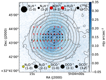
Figure 1: Multipointing grids and onion-shell model overlaid with the 850 $\mu$m  contour. The black and yellow dots in a ($\Delta$RA, $\Delta$Dec)=(12^′′, 12^′′)-spacing grid show the pointings of IRAM 30-m and GBT observations, respectively. The red dots in a ($\Delta$RA, $\Delta$Dec)=(15^′′, 30^′′)-spacing grid show those of JCMT HARP observations. The circles at top and bottom indicate the beam sizes of each spectral observations. The gray concentric circles with center of L1512 represent the onion-shell model with shell widths of 12^′′. The 850 $\mu$m  map is shown in blue-scale, and its white and black contours have the same levels as in Fig. 2g.

2 Observations and data reduction

Observational parameters are summarized in Table 1 and the pointings of spectral line observations are shown in Fig. 1.

2.1 IRAM 30 m observations

We observed L 1512 using the IRAM 30 m telescope in December 2013, May and October 2014, and September 2017. Five molecular lines were observed in frequency-switching mode using the dual polarization Eight MIxer Receiver (EMIR), the Versatile Spectral Autocorrelator (VESPA), and the Fourier Transform Spectrometer (FTS); these lines are N₂H⁺ (1–0), N₂H⁺ (3–2), N₂D⁺ (2–1), DCO⁺ (2–1), and DCO⁺ (3–2). The frequency resolution was adapted to keep the velocity sampling close to 50 m s^-1. Both polarizations are systematically averaged. The spectra were observed on a 12^′′ grid in an east-west strip 12^′′ south of the core center (RA, Dec)_J2000 = (5^h04^m07$\aas@@fstack{s}$5, +32°43^′ 25$\aas@@fstack{\prime\prime}$0) and along a north-south strip across the core center. Pointing was regularly checked every 1.5 hours and pointing error was monitored to be less than 3^′′. Data were subsequently folded and baseline subtracted with CLASS. The original cut passes 12^′′ south of the true center because when the project started the CFHT and SCUBA-II maps were not yet available and the core center position was not accurately known. Complementary observations in September 2017 (Director Discretionary Time) were performed. Two short east-west strips across the core center and 12^′′ above the center, and one short strip along the north-south strip (mentioned above) for N₂H⁺ (1–0) and DCO⁺ (2–1) allowed us to check that the modeling of the core is still consistent with the included offset. Figure 1 shows the pointings of spectral line observations, and the observational parameters are summarized in Table 1. We complemented our observations with on-the-fly (OTF) maps of N₂H⁺ (1–0) and C¹⁸O (2–1) obtained by Lippok et al. (2013), and multipointing mosaic maps of C¹⁸O (1–0) and ¹³CO (1–0) obtained by Falgarone et al. (1998). Lippok et al. (2013) and Falgarone et al. (1998) give observational details. The above data are regridded to supplement two orthogonal strips (Figs. 3 and 4) and measure the spectral center velocity (Fig. 5d) using a Gaussian fit routine in CLASS. We also produce the moment maps of N₂H⁺ (1–0) and C¹⁸O (1–0) (Figs. 2h,i and Figs. 5a,b). Among these, the N₂H⁺ moment maps include our observations and the OTF data.

2.2 JCMT observations

The N₂H⁺ (4–3) and H₂D⁺ (1₁₀–1₁₁) observations were carried out in December 2015 using the JCMT 15 m telescope and the 16 pixels HARP receiver (two pixels of which are non-functioning) in frequency–switching mode. Thanks to the proximity of the two lines (250 MHz), they are routinely observed together with two sub-bands from the Auto Correlation Spectral Imaging System (ACSIS) spectrometer. Data are converted to the CLASS format to be reduced with CLASS (folding and baseline subtraction). Observational parameters are summarized in Table 1, and the pointings of spectral line observations are shown in Fig. 1.

SCUBA-II observations were retrieved from the JCMT archive. They are part of the M13BC01 project (PI, James di Francesco). As far as we know, these data have not been published previously.

2.3 GBT observations

We observed L 1512 using the GBT 100 m off-axis telescope in November 2014. We used the MM1 (67–74 GHz) and MM2 (73–80 GHz) W-band dual polarization sub-band receivers in in-band frequency-switching mode with the Versatile GBT Astronomical Spectrometer (VEGAS) backend. Pointing was checked every hour and each session started with a surface shape verification by using Out Of Focus Holography (OOF) on a strong source. Data were preprocessed (calibrated, folded, and baseline subtracted) in the GBTIDL data reduction program and converted to CLASS format for subsequent reduction. Thanks to the very smooth baseline of the receiver (due to the use of large band amplifiers instead of mixers), the preprocessing of the data allows us to treat separately the ON and OFF observations (i.e., total power mode) and gain a factor of $\sqrt{2}$ on the noise (the method will be presented in a subsequent paper).

2.4 CFHT observations

The CFHT Wide InfraRed CAMera (WIRCAM) was used with the wide filters J, H, and $K_{s}$ to observe the source on the night of 26 December 2013. To preserve the extended emission (scattered light known as cloudshine; Foster & Goodman 2006), we used a SKY-TARGET-SKY nodding mode to subtract the atmospheric infrared emission. Seeing conditions were typically 0$\aas@@fstack{\prime\prime}$8. Data reduction was performed at the (now closed) TERAPIX center using a specific reduction method to recover the extended emission. The integration times were typically of 0.5 to 1 hour on-source per filter, to reach a completude magnitude of 21.5 (J band) to 20 ($K_{s}$ band). The extended emission will be analyzed in a subsequent paper.

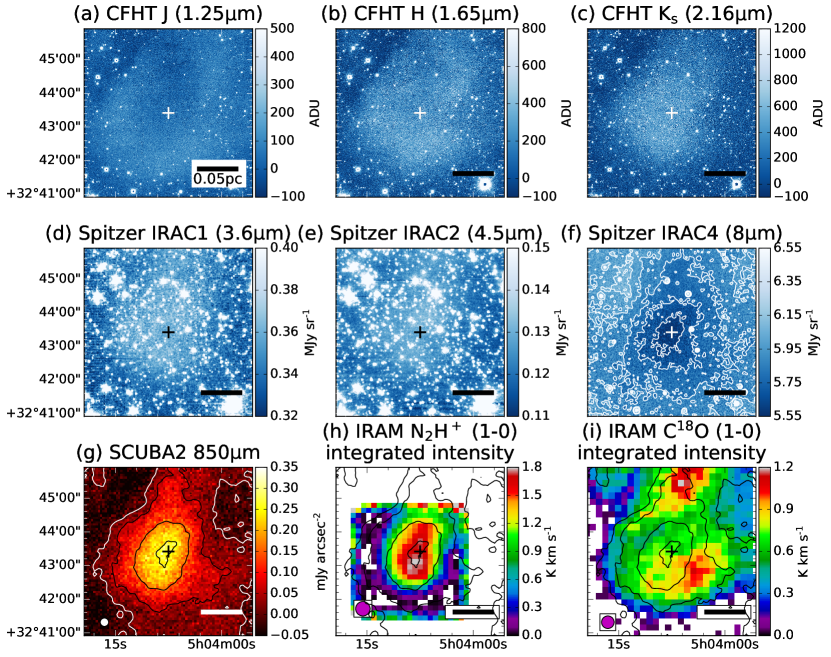
Figure 2: L1512 maps of continuum and line integrated intensity. The CFHT NIR maps at (a) J band, (b) H band, and (c) $K_{s}$ band. Spitzer MIR maps at (d) IRAC1 band, (e) IRAC2 band, and (f) IRAC4 band with its contours at 5.15, 5.25, 5.35, 5.45, 5.55 MJy/sr. (g) JCMT SCUBA map at 850 $\mu$m with its contours at 0, 0.05, 0.15, 0.25 mJy/arcsec². Integrated intensity maps of (h) N₂H⁺ $J$=1–0 and (i) C¹⁸O $J$=1–0 calculated within $V_{\rm LSR}$=[$-$3 km s^-1, 16 km s^-1] and [6.0 km s^-1, 7.5 km s^-1], respectively. The panels $h$ and $i$ are overlaid with contours from the the 850 $\mu$m  image. The central cross in each panel indicates the center of L1512 determined by the IRAC4 map. The scale bars of 0.05 pc and millimeter-wavelength beam sizes are denoted in the bottom right and bottom left corners, respectively.

2.5 Spitzer observations

Spitzer observations are collected from the Spitzer Heritage Archive (SHA). L 1512 was observed in two programs with Spitzer InfraRed Array Camera (IRAC), Program id. 94 (PI, Charles Lawrence) and Program id. 90109 (PI, Roberta Paladini); the second program occurred during the warm period of the mission (only 3.6 and 4.5 $\mu$m channels still working). The P94 data were already discussed in Stutz et al. (2009), while the warm mission data are analyzed in Steinacker et al. (2015). These two papers provide the presentation of the observations. During the warm mission, deep observations of the cloud were performed and a completed magnitude of 18 in band I2 (4.5 $\mu$m) was reached.

3 Results

3.1 Continuum maps

Figure 2 shows the continuum maps of L1512 at near-infrared (NIR), mid-infrared (MIR), and submillimeter (submm) wavelengths. The NIR maps of L1512 at J, H, and $K_{s}$ bands (Figs. 2a–c) reveal extended emission that is distributed from an annular shape at J band and progressively merges to a concentrated shape at $K_{s}$ band. These structures are caused by the scattered light of ambient interstellar radiation field by dust grains ($a_{\rm gr}\sim 0.1$ $\mu$m) at the periphery of L1512. Similar structures in dark clouds in the Perseus molecular complex have been found and studied by Foster & Goodman (2006) and Juvela et al. (2006). Foster & Goodman (2006) introduced this scattering effect as cloudshine, and proposed to use it as a general tracer of the column density of dense clouds. Since the wavelength of the maximum scattering cross section increases with the size of dust grains, the different spatial spread of the cloudshine of L1512 at the three bands also indicates that the dust grains have the smallest size at the outskirts, and become larger toward the inner region as discussed in Steinacker et al. (2010) and Lefèvre et al. (2014, 2016).

On the other hand, the MIR maps of L1512 from IRAC1 and IRAC2 bands (Figs. 2d,e) show a more compact emission feature, while the IRAC4 map (Fig. 2f) shows absorption instead. The absorption feature is mainly caused by the bright PAH emission from the diffuse medium, the extinction of which becomes superior to the inner scattered light contribution (Lefèvre et al., 2016). The similar spatial distributions between the compact emission and absorption indicate that the emission also comes from the central core. Pagani et al. (2010b) and Steinacker et al. (2010) firstly recognized this phenomenon in their sample of nearby starless and Class 0/I protostellar cores. By analogy to cloudshine, they named this effect coreshine. With the benefit of the smaller beam sizes of IRAC maps compared with those of JCMT SCUBA maps, we determined the center of L1512 core at (RA, Dec)_J2000 = (5^h04^m07$\aas@@fstack{s}$5, +32°43^′ 25$\aas@@fstack{\prime\prime}$0) using IRAC4 band (8 $\mu$m) with a beam size of 2^′′, and denote it as a cross shown in each panel of Fig. 2.

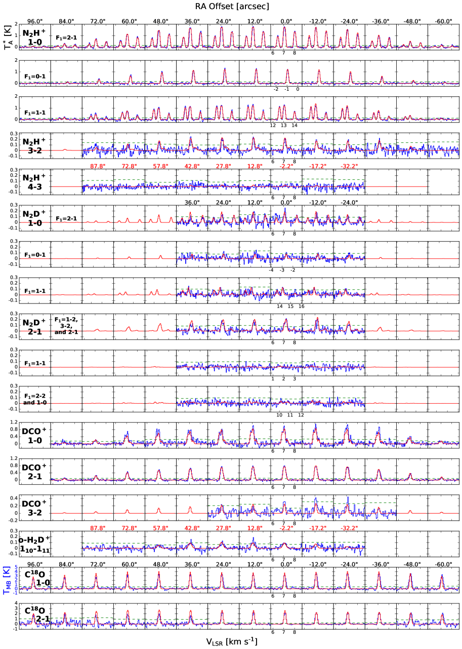
Figure 3: Spectral observations along the main horizontal cuts at $\Delta$Dec=$-$12^′′ (IRAM/GBT) or $-$16^′′ (JCMT) compared to our best-fit radiative transfer model. The blue spectra show the observational data, and the red spectra show the models. Each column corresponds to different horizontal offsets from the center of L 1512 according to Fig. 1. Each row shows a spectral line, except that the N₂H⁺ (1–0), N₂D⁺ (1–0) and (2–1) lines are split into three rows corresponding to their different $F_{1}$-transition groups. For C¹⁸O (2–1), our data are supplemented with OTF spectra from previous works at large offsets. The green dashed lines indicate the three $\sigma$ noise level.

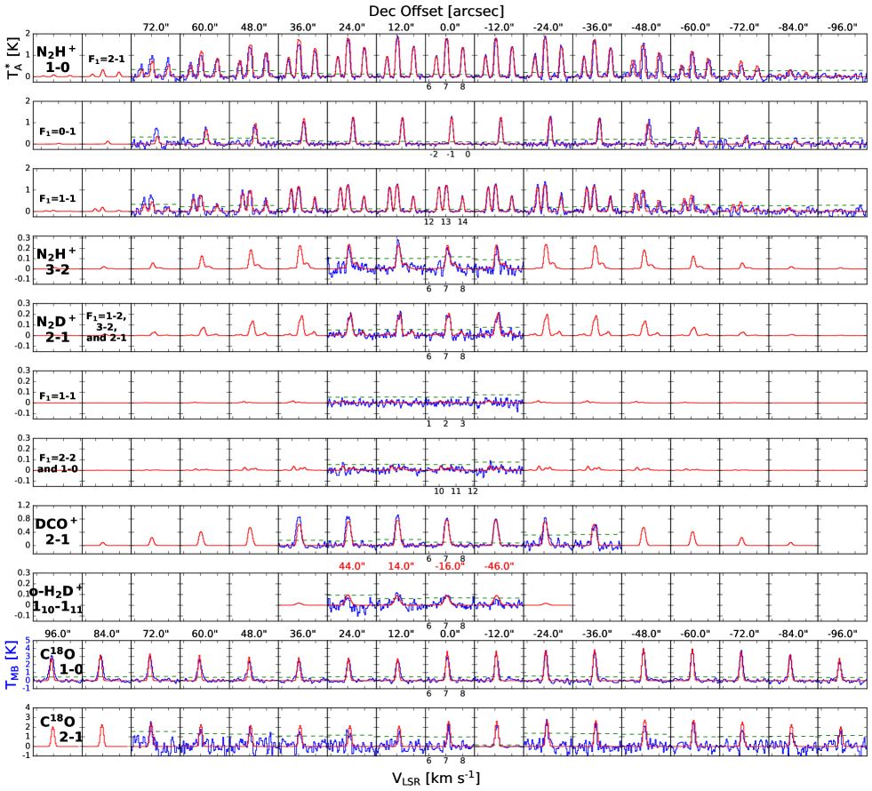
Figure 4: Spectral observations along the main vertical cuts at $\Delta$RA=0^′′ (IRAM/GBT) or $-$2.2^′′ (JCMT) compared to our best-fit radiative transfer model. For N₂H⁺ (1–0) and C¹⁸O (2–1), our data are supplemented with OTF spectra from previous works at large offsets. Other annotations are the same as in Fig. 3.

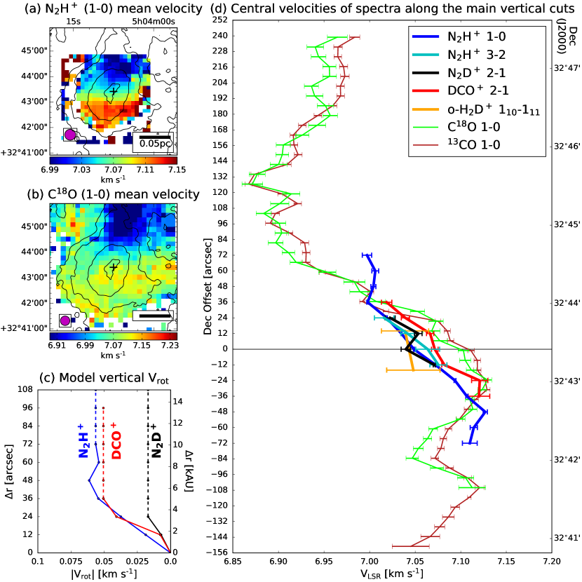
Figure 5: Velocity structure. Mean velocity maps of (a) the $F_{1}F$=2,3–2,1 component of N₂H⁺ $J$=1–0 and (b) C¹⁸O $J$=1–0 calculated within $V_{\rm LSR}$=[6.75 km s^-1, 7.50 km s^-1] and [6.0 km s^-1, 7.5 km s^-1], respectively. Contours from the the 850 $\mu$m  image are overlaid. The rest of the symbols in the panels $a$ and $b$ have the same meaning as in Fig. 2. (c) Model vertical rotation velocities, $V_{\rm rot}$, against radius, $\Delta$r, adopted in the radiative transfer model. (d) Central velocities and their error bars of the spectra along the main vertical cuts. Two $y$-axes are vertical offsets to the center and declination, respectively.

3.2 Molecular emission lines

Figure 1 shows the pointings of spectral line observations using IRAM 30 m, GBT, and JCMT HARP. Horizontally, our IRAM/GBT observations at $\Delta{\rm Dec}=-12$^′′ and our JCMT observation at $\Delta{\rm Dec}=-16$^′′ have the widest coverage across the L1512 core. Vertically, our IRAM/GBT observations at $\Delta{\rm RA}=0$^′′ have the widest coverage, and the JCMT observation closest to it is at $\Delta{\rm RA}=-2$$\aas@@fstack{\prime\prime}$2. We used these cuts (hereafter referring to them as the main horizontal cuts and the main vertical cuts) to analyze the physical and chemical properties of L1512 (Sect. 4). Figures 3 and 4 show the spectra of each emission line in the $T_{\rm A}^{*}$ scale (except for C¹⁸O (1–0) in the $T_{\rm MB}$ scale) along the main horizontal and vertical cuts, respectively.

Since L1512 is a quiescent starless core, each hyperfine component of N₂H⁺ (1–0) and N₂D⁺ (1–0) is well separated with line widths of $\sim$0.2 km s^-1. Along the main horizontal cuts, the coverage of the N₂H⁺ (1–0) spectra includes the whole starless core with the intensity peak toward the central region. Likewise, the spectra of N₂H⁺ (3–2), N₂D⁺, and DCO⁺ also peak toward the central region, which suggests that these four cations trace the dense core region. In addition, our highest observed transition of N₂H⁺, the $J$=4–3 line, shows no signal according to the 3$\sigma$ criterion with a rms noise level of $\sim$30 mK because of the low kinetic temperature in the core region and low density compared to the requested critical density for this transition (two orders of magnitude lower). Among the four cations, the ortho-H₂D⁺ (1₁₀–1₁₁) line is detected in a smaller spatial region ($\Delta{\rm RA}=-$17.2^′′ to 42.8^′′), which indicates that ortho-H₂D⁺ traces the innermost region of the L 1512 core. On the other hand, the intensity of the C¹⁸O (1–0) and (2–1) spectra are relatively constant across the inner core, which is a clear indication that C¹⁸O is depleted across the whole core.

Along the main vertical cuts, Fig. 4 shows that N₂H⁺, N₂D⁺, and DCO⁺ are also depleted in the innermost region. Their spectral peaks drop between the region from $\Delta{\rm Dec}=-$24 to $+$12^′′ for which the intensity decrements range from 0.04 to 0.15 K with $\sim$2–5$\sigma$ significant levels, while they should increase to follow the increase of column density toward the center if there were no depletion. Similarly, the ortho-H₂D⁺ spectra show a roughly constant intensity across the peak, which is a sure sign of depletion since the line is optically thin and should be roughly proportional to the H₂ column density. The depletion effects are also found in the integrated intensity maps of N₂H⁺ (1–0) and C¹⁸O (1–0) shown in Figs. 2h and i. The C¹⁸O emission clearly shows depletion toward the center of the cloud because the peak emission is situated on the outskirts, while an offset between N₂H⁺ emission peak and dust peak suggests that N₂H⁺ also depletes in the innermost region.

3.3 Velocity structure

Figures 5a and b show the mean velocity maps of L 1512, which reveals a velocity gradient in the north-south direction. The constant gradient inside the core itself is compatible with a rigid-like rotation feature or could be due to an oscillation of the whole filament. Figure 5d shows the central velocity of each spectral line along the main vertical cuts fitted with the CLASS Gaussian fitting task. The hyperfine structures of the N₂H⁺, N₂D⁺, and DCO⁺ rotational lines are taken into account for the fitting. We see that the N₂H⁺ (1–0) emission appears to have a rather uniform velocity gradient of 2.26 $\pm$ 0.04 km s^-1 pc^-1 between $\Delta{\rm Dec}=-48$^′′ and $+$36^′′, which is compatible with a rigid body rotation. The N₂H⁺ (3–2), N₂D⁺ (2–1), DCO⁺ (2–1), (and possibly ortho-H₂D⁺ (1₁₀–1₁₁) although its velocity measurement is hampered by a low signal-to-noise ratio) emissions also have similar dynamical behaviors. The C¹⁸O (1–0) and ¹³CO (1–0) data from Falgarone et al. (1998) partially follow the ionic species velocity drift but with an offset of $\sim$50 m s^-1 toward the center. Because the ¹³CO emission traces a more extended region than C¹⁸O, the similarity between the C¹⁸O and ¹³CO emissions might be due to C¹⁸O depletion in the core region and its emission being dominated by the L 1512 envelope. The CO isotopolog redshift by $\sim$50 m s^-1 toward the center could be explained by a contraction of the envelope, if the line is optically thick enough to mask the corresponding blueshifted component that we would expect on the back side of the cloud; however, this seems difficult to justify for the C¹⁸O (1–0) transition. The other possible explanation is that the envelope is experiencing an oscillation in which the core is coupled to it with a delay and is presently toppling over. This kind of oscillation has been proposed to explain the Orion and the G350.54+0.69 filaments (Stutz et al., 2018; Liu et al., 2019) and has also been invoked for L 1512 itself (Lee et al., 2001; Sohn et al., 2007; Lee & Myers, 2011).

4 Analysis

Our first step is to analyze the dust absorption maps from 1.2 $\mu$m to 4.5 $\mu$m to estimate the total column density of gas+dust all over the cloud. We converted this map into a sphere on first-order approximation to analyze the line emissions. We adopted a correspondingly 1D spherically symmetric non-LTE radiative transfer code (Bernes, 1979; Pagani et al., 2007) to reproduce our observed emission line spectra. Since the shape of L 1512 is globular, we can assume that its distributions of volumetric number density ($n_{\rm H_{2}}$), gas kinetic temperature ($T_{\rm kin}$), volumetric relative abundances with respect to H₂ of the observed species ($X_{\rm species}=n_{\rm species}/n_{\rm H_{2}}$) and turbulent velocity ($V_{\rm turb}$) can be approximated by an onion-shell structure composed of multiple concentric homogeneous layers. We note however that the cloud is slightly dissymmetric and we used two slightly different models to describe the east and west sides of the cloud. In addition, rotational velocity field ($V_{\rm rot}$) and radial velocity field ($V_{\rm rad}$) can also be applied to each layer. We chose the widths of the layers to be 12^′′ (=1,680 AU), which is the smaller spacing of the two pointing-grids (Fig. 1). The advantage is that we can determine the physical parameters and chemical abundances at each layer sequentially from the outermost to the innermost layer by sampling sightlines of progressively decreasing radius along a cut across L 1512.

Our procedure to determine $n_{\rm H_{2}}$, $T_{\rm kin}$, $X_{\rm species}$, and $V_{\rm turb}$ of each layer is as follows. First, the $n_{\rm H_{2}}$ profile was determined independently from an extinction map. Second, we used N₂H⁺ data to determine their $T_{\rm kin}$, $X$(N₂H⁺), and $V_{\rm turb}$ profiles. Third, we assumed that all the other species have the same $T_{\rm kin}$ and $V_{\rm turb}$ profiles as those of N₂H⁺ to determine the abundance profiles of N₂D⁺, DCO⁺, and ortho-H₂D⁺. Given the abundance profiles of the various ions, we adopted a pseudo time-dependent chemical model (Pagani et al., 2009b) to estimate the lifetime scale of each layer with our derived $n_{\rm H_{2}}$ and $T_{\rm kin}$, and we also derived the abundance profiles of their parent species, CO and N₂.

4.1 Visual extinction

We adopted the Near-Infrared Color Excess Revisited technique (NICER; Lombardi & Alves, 2001) to derive the visual extinction, $A_{\rm V}$, with color excesses of stars from NIR and MIR bands. Since the NIR data preferentially trace the diffuse region, we used the $R_{\rm V}=3.1$ model from Weingartner & Draine (2001) to derive the $A_{\rm V}$ map of the envelope (Fig. 6a) using J, H, and $K_{s}$ bands. On the other hand, the MIR data preferentially trace the dense region. We alternatively used the $R_{\rm V}=5.5$ case B model from Weingartner & Draine (2001) to derive $A_{\rm V}$ map of the core region (Fig. 6b) using H, $K_{s}$, and IRAC2 bands. The case B model is an improved variant of the $R_{\rm V}=5.5$ model from Weingartner & Draine (2001), but characterizes the denser region better (by including spherical grains up to 10 $\mu$m in size), although not perfectly (Cambrésy et al., 2011; Ascenso et al., 2013). Thanks to the deep sensitivity of the CFHT and Spitzer observations, the density of stars across the cloud core is high enough to convolve the reddening data with a 2D Gaussian profile of half-power beam width (HPBW) as small as 30^′′ to construct the maps. The dense core map traces the central region better than the diffuse envelope map but could not properly trace the outer low-$A_{\rm V}$ region, and vice versa. In order to combine these two maps, we calculated the azimuthally-averaged $A_{\rm V}$ profiles of the envelope and core maps shown in Fig. 6d from the 1^′ horizontal strip across the center (Figs. 6a,b) to avoid the cometary tail. We could see that the two profiles merge at $\sim$2.5 mag and become similar in the outer region. Therefore, an $A_{\rm V}$ threshold of 2.5 mag is used to combine the central region from the core map and the outer region from the envelope map, and the result is shown in Fig. 6c.

4.2 Density profile

The volume density ($n_{\rm H_{2}}$) profile of L 1512 is modeled with the spherically symmetric Plummer-like profile,

$$n_{\rm H_{2}}(r)=\begin{dcases}\frac{n_{0}}{1+\big{(}\frac{r}{R_{0}}\big{)}^{\eta}}&\text{if $r\leq R_{\rm edge}$}\\ 0&\text{otherwise,}\end{dcases}$$ (1)

where $n_{0}$ is the central density, $R_{0}$ is the characteristic radius, $\eta$ is the power-law index of $n_{\rm H_{2}}$ profile as $r\gg R_{0}$, and $R_{\rm edge}$ is set as 320^′′ ($=$44,800 AU) to cover the whole core. Since the contribution from the diffuse envelope is small compared with the dense core, we simply adopted the $R_{\rm V}=5.5$B model for the conversion of the extinction, $A_{\rm V}$, into column density, $N_{\rm H_{2}}$. Therefore we obtain a relation between $A_{\rm V}$ and $N_{\rm H_{2}}$ (Bohlin et al., 1978),

$$N_{\rm H_{2}}/A_{\rm V}=5.3\times 10^{20}\text{ cm${}^{-2}$\, mag${}^{-1}$.}$$ (2)

In order to derive $n_{0}$, $R_{0}$ and $\eta$ in the volume density model of L 1512, we produced an $A_{\rm V}$ model map by (1) integrating a Plummer-like $n_{\rm H_{2}}$ model along the line of sight and convolving it with the same beam size as the combined $A_{\rm V}$ map (Fig. 6c) to obtain an $N_{\rm H_{2}}$ model map, and then (2) derive an $A_{\rm V}$ model map using Eq. 2. Therefore, we could perform a fitting on the azimuthally-averaged profiles of the $A_{\rm V}$ model map and the combined $A_{\rm V}$ map with the Levenberg-Marquardt algorithm included in the Python scipy.optimize.curve_fit function.

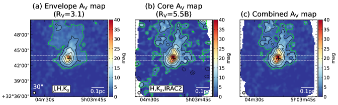
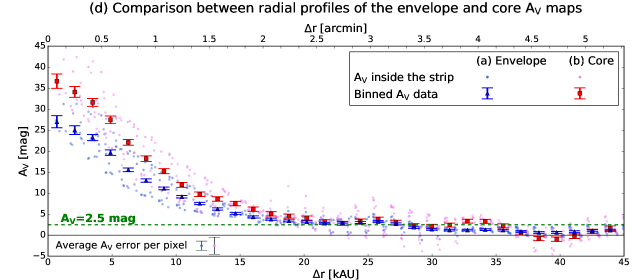
Figure 6: Visual extinction maps and profiles. (a) Envelope $A_{\rm V}$ map derived from J, H, and $K_{s}$ bands with the $R_{\rm V}=3.1$ model. (b) Core $A_{\rm V}$ map derived from H, $K_{s}$, and IRAC2 bands with the $R_{\rm V}=5.5$B model. (c) Combined $A_{\rm V}$ map merged from the previous maps with boundaries at $A_{\rm V}=2.5$ mag. Each map is convolved with a Gaussian beam size of 30^′′. (d) Comparison between $A_{\rm V}$ profiles inside the strips of panel $a$ and $b$. The $A_{\rm V}$ values at each pixel are denoted in light blue and pink dots, while their average errors are indicated in the bottom left corner. The $A_{\rm V}$ profiles are averaged in azimuth with radial 10^′′ bin and shown in blue triangles and red squares with their error bars. The green dashed lines in the four planes indicate the $A_{\rm V}$ threshold of 2.5 mag.

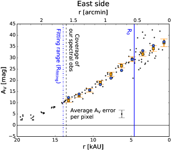
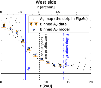
Figure 7: Plummer-like density profile fittings. The black dots are the $A_{\rm V}$ values at each pixel in the horizontal strip shown in Fig. 6c but these are separated between the east and west sides. The orange squares with error bars show the averaged $A_{\rm V}$ profiles, which are azimuthally binned with radial 10^′′ bin. The blue circles show the best-fitted $A_{\rm V}$ models for the east and west sides. The $A_{\rm V}$ models are derived from spherically symmetrical Plummer-like density profiles. The best-fitted characteristic radii, $R_{0}$, and the fitting ranges, $R_{\rm fitting}$ of the $A_{\rm V}$ models are denoted in blue solid and dash-dotted lines, respectively. The coverage of our spectral observations are denoted in black dashed lines.

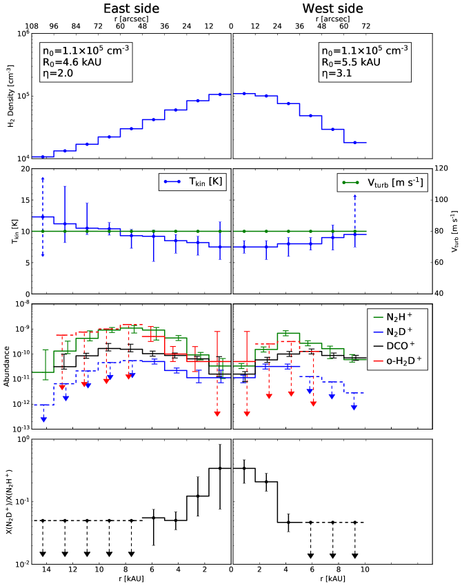
Figure 8: Physical and abundance profiles. The Plummer-like density ($n_{\rm H_{2}}$) profiles are derived from the combined extinction map (Fig. 6c), where the best-fit parameters are annotated. The profiles of kinetic temperature ($T_{\rm kin}$), turbulent velocity ($V_{\rm turb}$), abundances ($X_{\rm species}$), and the abundance ratio of N₂D⁺/N₂H⁺ are the best-fit results from the non-LTE radiative transfer calculations.

Figure 7 shows the fitting results for the east and west sides of L 1512 using the $A_{\rm V}$ computed in the strip shown in Fig. 6c, which spatially covers the main horizontal cuts. In order to ensure that the volume density models of both sides agree with each other at the center, $n_{0}$ was previously fitted by an averaged profile from both sides. Then $n_{0}$ was fixed in the individual fitting for each side. These determined parameters and volume density profiles are shown in the first row in Fig. 8. We see that the horizontal $n_{\rm H_{2}}$ profile is skewed in such a way that it is steeper on the west side than the other side. The volume densities drop to $\sim$10⁴ cm^-3 at both edges of our spectral observation coverage.

4.3 Radiative transfer applied to the onion-shell model

We assumed an onion-shell model comprised of nine and six 12^′′ layers in thickness on the east and west sides, respectively. Then we reproduced the spectra of N₂H⁺ (1–0, 3–2, and 4–3) along the main horizontal cuts with the 1D spherically symmetric non-LTE radiative transfer code (Pagani et al., 2007) by varying $T_{\rm kin}$, $X$(N₂H⁺), $V_{\rm turb}$, $V_{\rm rot}$, and $V_{\rm rad}$ at each layer. Here we used the para-H₂–N₂H⁺ collisional coefficients instead of the original He–N₂H⁺ hyperfine collisional coefficients (Lique et al., 2015). We also used specific para-H₂–N₂D⁺ collisional rate coefficients for the deuterated isotopolog (see Appendix B). One of the important features of this code is that the line overlap between hyperfine transitions at close frequencies is taken into account to calculate the correct spectral line shape and excitation. Among the input parameters, $V_{\rm turb}$, $V_{\rm rot}$, and $V_{\rm rad}$ are determined from observations. We set both $V_{\rm rot}$ and $V_{\rm rad}$ to zero, since the L 1512 core has no obvious infall/expansion motion and only a vertical rotational component, while our model follows the RA (horizontal) structure. For $V_{\rm turb}$, we found that a uniform turbulent velocity of 80 m s^-1 could reproduce the spectral line widths along the cuts. Afterward, we performed an iterative spectral fitting procedure to obtain $T_{\rm kin}$ and $X$(N₂H⁺) profiles, taking care to eliminate nonphysical solutions such as parameter oscillations between layers, even if they provide better $\chi^{2}$.

An important feature of our approach is that instead of converting the data into the $T_{\mathrm{MB}}$ scale for direct comparison with the non-LTE model, which is absolutely not valid for extended regions such as starless clouds, we reproduce the observations by computing the telescope coupling to the sky, based on its main beam, error beams, and forward scattering and spillover efficiency ($\eta_{\mathrm{fss}}$). We then obtained our model predictions directly calibrated in the $T_{\mathrm{A}}^{*}$ scale, whereas the $T_{\mathrm{MB}}$ scale is overcorrected for low $\eta_{\mathrm{MB}}$ values such as those found for the IRAM 30 m in the 1.3–0.8 mm range since the error beams pick up a substantial fraction of the signal when the source is extended. This leads to wrong line ratios and overestimates of the temperature and/or density of the cloud and also has an impact on the species abundance.

Once the density, temperature, and kinematic properties of the onion-shell model were constrained by the N₂H⁺ modeling, we reproduced the spectra of N₂D⁺ (1–0, and 2–1), DCO⁺ (1–0, 2–1, and 3–2), and ortho-H₂D⁺ (1₁₀–1₁₁) by varying only their abundances and assuming that they share the same physical parameters as N₂H⁺. Similarly, $X$(N₂D⁺), $X$(DCO⁺), and $X$(ortho-H₂D⁺) profiles were obtained using the above iteratively spectral fitting procedure. Since we lacked N₂D⁺ observations at large radii, we set upper limits of $X$(N₂D⁺) in the outer layers from $X$(N₂H⁺) multiplied by the minimum observed $X$(N₂D⁺)/$X$(N₂H⁺ $)=0.05$. For the non-detection observations of ortho-H₂D⁺, we also estimated their abundance upper limits.

Figure 8 shows the profiles of $T_{\rm kin}$, $V_{\rm turb}$, abundances of the above four cations, and the N₂H⁺ fractionation, $X$(N₂D⁺)/$X$(N₂H⁺). The above best-fit profiles are also numerically listed in Table 10. The error bar in each layer is determined by the range of quantity, where

$$\Delta\chi^{2}=\chi^{2}(\text{quantity})-\chi^{2}(\text{the best-fit quantity})\leq 1.$$ (3)

We only determined the upper limit of $X$(ortho-H₂D⁺) toward the innermost layer. A higher signal-to-noise ratio of ortho-H₂D⁺ would be needed to derive its lower limit because the volume of the innermost layer is the smallest and its contribution to the emergent intensity is also small.

Finally, the best-fit modeled spectra of the four cations along the main horizontal cuts are shown in red in Fig. 3. The fit with the observed spectra is remarkably good. To see if the observed spectra along the main vertical cut could also be reproduced by our onion-shell model, we simply assumed that the physical parameters and abundance profiles were the same as those of the east side except for $V_{\rm rot}$ profile that is now not zero. Since the L 1512 core has a vertical motion compatible with a solid-body rotation, we adopted the $V_{\rm rot}$ profile of N₂H⁺, N₂D⁺, and DCO⁺ shown in Fig. 5c, which averages the central velocities of the vertical spectra (Fig. 5d) between the north and south sides. For ortho-H₂D⁺, we simply adopted the $V_{\rm rot}$ profile of N₂H⁺ because of its weak detection. The above $V_{\rm rot}$ profiles are given at layer interfaces and the rotational velocity inside a layer is linearly interpolated between the two given velocities at the inner and outer sides of that layer. The modeled spectra of the four cations are shown in red in Fig. 4, and are again in good agreement with the observations. Our results suggest that the 1D spherically symmetric assumption is globally valid for L 1512.

4.4 Time-dependent chemical model

We adopted a pseudo time-dependent gas-phase chemical model (Pagani et al., 2009b) to reproduce the deuteration ratio, $X$(N₂D⁺)/$X$(N₂H⁺), and abundances of N₂H⁺, N₂D⁺, DCO⁺, and ortho-H₂D⁺ in each layer. In the pseudo time-dependent approach, the physical properties ($n_{\rm H_{2}}$, $T_{\rm kin}$) are kept constant while the chemical abundances ($X_{\rm species}$) evolve. We considered a chemical network, where (1) different spin states (ortho, para, and meta) of H₂ and H${}_{3}^{+}$, and their isotopologs are all included, and (2) heavy molecules are totally depleted except for CO and N₂ which are partially depleted.

The initial ortho-H₂/para-H₂ ratio is assumed to be their statistical weights of 3:1 and H${}_{3}^{+}$ is formed later via the cosmic ray ionization of H₂. After the ortho/para ratio (OPR) of H₂ has dropped to values low enough to prevent destruction of H₂D⁺ by ortho-H₂ (OPR $\lesssim$ 1% or less; Pagani et al. 1992a, 2009b), the deuterium fractionation of H${}_{3}^{+}$ enhances in the low $T_{\rm kin}$ and highly depleted environment, forming H₂D⁺, and subsequently D₂H⁺ and D${}_{3}^{+}$. Then H${}_{3}^{+}$ and its isotopologs transfer protons/deuterons to CO and N₂ and produce HCO⁺, DCO⁺, N₂H⁺, and N₂D⁺. HCO⁺ is not a suitable tracer for starless cores because its low rotational transition emission is optically thick and this ion is present in both the envelope and the core (which is also true for H¹³CO⁺ and HC¹⁸O⁺), while ortho-H₂D⁺, DCO⁺, N₂H⁺, and N₂D⁺ emissions are optically thinner and most importantly are confined to the core (Pagani et al., 2012). Since we evaluated the quasi-instantaneous conversion of CO and N₂ into the aforementioned ions, we can assume that their abundances are in equilibrium with these ions locally. Therefore, the gas-phase abundances of these two neutral molecules are free parameters in our chemical model. The other free parameters are the average grain size ($a_{\rm gr}$) and the cosmic ray ionization rate ($\zeta$).

Figure 9 shows the chemical model solutions of $X$(ortho-H₂D⁺), $X$(N₂D⁺)/$X$(N₂H⁺), and $X$(DCO⁺) for each layer toward the east and west sides. Typical $\zeta$ of 10^-17 s^-1 was adopted throughout the chemical model. For $a_{\rm gr}$, although Steinacker et al. (2015) find that the maximum spherical grain size can reach $\sim$0.5 $\mu$m in this source, the majority of the grains are still small and the larger grains have fluffy surfaces (e.g., Tazaki et al., 2016), therefore limiting the decrease of the total grain surface cross section. The impact on the chemistry and the freeze-out time should be negligible compared to the standard 0.1 $\mu$m grain size usually adopted in chemical models. In each layer, $X$(CO) and $X$(N₂) were adjusted to make the chemical solutions of the four cations fit the observed abundances (or remain below the observed upper limits) simultaneously. We found that the time ranges for all layers meeting the observations are 0.2–2.6 Myr for the east side and 0.2–1.9 Myr for the west side.

Figure 10 shows the derived CO and N₂ abundance profiles, while their values are listed in Table 10. Although the isotopologs of CO are not considered in our chemical network, we can obtain the $X$(C¹⁸O) profile through a ¹²C¹⁶O/¹²C¹⁸O abundance ratio in the layers in which C¹⁸O cannot be measured directly. In the outer region, where radiative transfer modeling is applicable, we find that the C¹⁸O abundance is $1\times 10^{-7}$ up to a radius of 3^′ (=25,200 AU). Since $X$(C¹⁸O) is limited to $1\times 10^{-7}$ toward the sixth eastern layer, where the ¹²CO abundance reaches its maximum of $5\times 10^{-5}$, we find an isotopolog ratio of ¹²C¹⁶O/¹²C¹⁸O = 500. This is compatible with the local ¹⁶O/¹⁸O ISM ratio of 557$\pm$30 (Wilson & Rood, 1994). As there is no reason to vary this ratio across the cloud, we obtained the inner C¹⁸O abundance profile between the fifth eastern and the third western layers by applying the same ratio of 500 to $X$(¹²CO) profile. On the other hand, the outer ¹²CO abundance profile is kept as high as $5\times 10^{-5}$ because $X$(¹²CO) is poorly determined from the chemical model when both $X$(N₂D⁺)/$X$(N₂H⁺) and $X$(ortho-H₂D⁺) are only upper limits. As a result, we were able to reproduce the C¹⁸O spectra via the non-LTE radiative transfer calculation. Owing to the nonsymmetrical velocity shift of C¹⁸O, we adjusted the velocity offset of the modeled spectra individually on each spectrum based on the observations. The impact on the line shape is too small to be detectable. The northern C¹⁸O abundance profile (positive offsets) is different from the east-west profile and had to be decreased by a factor of 2–16 to fit the observations. This suggests a larger CO depletion toward the northern tail. It turns out that the observations can be fitted by our model results of C¹⁸O (1–0) and (2–1) along the main horizontal cut (Fig. 3) and main vertical cut (southward only, Fig. 4) computed with the abundances derived from the chemical model, thereby validating our chemical model results.

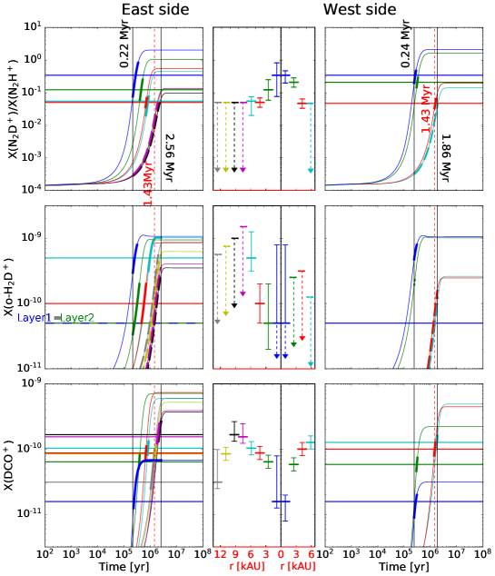
Figure 9: Chemical modeling of the abundance ratio of N₂D⁺/N₂H⁺ and the abundances of ortho-H₂D⁺ and DCO⁺ for each layer. The left and right columns show the chemical solutions, while the middle column shows the profiles. Each color represents a layer. In the chemical solution plots, the horizontal solid lines are the observationally derived $X$(N₂D⁺)/$X$(N₂H⁺), $X$(ortho-H₂D⁺), and $X$(DCO⁺). The growing curves are the chemical solutions calculated with an average grain size ($a_{\rm gr}$) of 0.1 $\mu$m and a cosmic ray ionization rate ($\zeta$) of 10^-17 s^-1. The two black vertical lines in each panel indicate a time range for which the model values cross the observations within their error bars and where the model curves become thicker. Thick dashed lines denote the model range that is both lower than the observed upper limit for that layer and within the global time range of the model. The red dashed vertical lines indicate the lower limit on the lifetime scale of L1512.

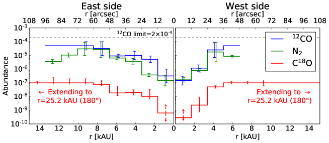
Figure 10: ¹²CO, N₂, and C¹⁸O abundance profiles. The ¹²CO and N₂ abundance profiles are the best-fit results from the chemical modeling. The C¹⁸O abundance profile is obtained by assuming a ¹²CO/C¹⁸O abundance ratio of 500 or a constant value of 1.0 $\times 10^{-7}$ extending to 25.3 kAU.

5 Discussion

As shown in Sect. 4, we built an onion-shell model of L 1512 to represent its physical structure ($n_{\rm H_{2}}$, $T_{\rm kin}$, and $V_{\rm turb}$ are shown in Fig. 8; $V_{\rm rot}$ in Fig. 5c) and chemical abundances (N₂H⁺, N₂D⁺, DCO⁺, and ortho-H₂D⁺ are shown in Fig. 8; CO, C¹⁸O, and N₂ in Fig. 10). Our model reproduces all the observed spectra along the main horizontal and vertical cuts (Figs. 3 and 4) via the non-LTE radiative transfer calculations. In this section, we first compare our findings with other studies and then address the lifetime of L 1512.

5.1 Density and kinetic temperature

By integrating the Plummer profile to the edge of the cloud where it merges in extinction with the background ($\sim$320^′′ from center), we find a peak $N_{\rm H_{2}}$ of $2.3\times 10^{22}$ cm^-2 toward the center of L 1512, which is higher than previously reported ($0.8-1.3\times 10^{22}$ cm^-2; Lee et al. 2003; Lippok et al. 2013, 2016). From the non-LTE modeling of both C¹⁸O and N₂H⁺ we also find 2.1 $\times 10^{22}$ cm^-2 in a 180^′′ radius, which is a lower limit since the cloud is truncated to the C¹⁸O emission extension and is consistent with the Plummer profile. This discrepancy is due to our different approach to derive the total column density. We use dust extinction, which is independent of the dust temperature ($T_{\rm dust}$), and N₂H⁺ modeling for which the uncertainty on the collisional coefficients is extremely small compared to the uncertainty on dust properties in emission at long wavelengths. On top of dust properties uncertainties, it is well known that the problem of quantifying dust in emission is degenerate. This is because of the unconstrained temperature variation along the line of sight that can hardly be disentangled from dust property variations and the nonlinearity of the blackbody intensity with temperature for the combination of wavelengths and temperatures of concern in starless cores (Pagani et al., 2015). Indeed, Lee et al. (2003) and Lippok et al. (2013, 2016) performed their estimations with dust thermal emission by assuming a constant $T_{\rm dust}$ of 10 K or using a decreasing $T_{\rm dust}$ toward the core center. However, their $N_{\rm H_{2}}$ are less than $\sim$50% of our result. Pagani et al. (2015) suggest that if only dust continuum data are used, $T_{\rm dust}$ can be overestimated and consequently the column density of starless cores can be underestimated. This is because warmer dust emission can easily dominate over cold dust emission in the spectral energy distribution fitting.

For the kinetic temperature, we find a central $T_{\rm kin}$ of 7.5$\pm{1}$ K on the west side, which is better constrained that the central temperature for the east side (7.5${}_{-2}^{+4}$ K) . We also note that the second central layer on the east side is better constrained too ($8.2_{-2}^{+1}$ K). Thus, we conclude that $T_{\rm kin}$ is down to 7.5$\pm{1}$ K in the center and rises to $\sim$10–17 K in the outer region. Because dust-gas coupling is efficient enough for $n_{\rm H_{2}}>10^{4.5}$ cm^-3 (Goldsmith, 2001), we can assume that $T_{\rm dust}=T_{\rm kin}$ in the core center based on our modeling. The central $T_{\rm dust}$ is therefore lower than Lippok et al. (2013, 2016)’s 9.8–11.3 K, which explains our peak column density discrepancy as already noticed in other sources by Pagani et al. (2015).

5.2 Cation abundance profiles

We find that N₂H⁺ is significantly depleted at the center of L 1512 ($n_{\rm H_{2}}=1.1\times 10^{5}$ cm^-3) and its abundance starts to decrease at $n_{\rm H_{2}}$ of 3 (east) to 8 (west) $\times 10^{4}$ cm^-3. This is one order of magnitude lower than toward L 183. By averaging the depletion factors calculated for the east and west sides, we obtain an averaged N₂H⁺ depletion factor of 27${}^{+17}_{-13}$, which is larger than the factor of 6${}^{+13}_{-3}$ in L 183 previously found by Pagani et al. (2007) while L 183 even has a denser central $n_{\rm H_{2}}\geq 2\times 10^{6}$ cm^-3. Strangely, Lee et al. (2003) suggests that N₂H⁺ may be depleted in L 1512 but not in another advanced and denser starless core, L 1544 ($n_{\rm H_{2}}\geq 10^{6}$ cm^-3) whereas Redaelli et al. (2019) present new observations and analysis of L 1544 for which they report a large volumetric depletion factor ($>$ 100). For N₂D⁺, we find a depletion factor of 4${}^{+2}_{-1}$, which is also higher than the factor of 2–2.5 found in L 183 (Pagani et al., 2007) but lower than the one reported for L 1544 by Redaelli et al. (2019), $\sim$15. It is surprising that the depletion factors do not correlate with the peak density among these three sources. One of the possibilities is that the dust grain size in L 1512 might be smaller than in the other cores keeping the depletion timescale shorter (Lee et al., 2003). Another possibility is the time it took to form the cores. L 183 seems to have contracted more rapidly than the two other cores ($\leq$0.7 Myr for L 183, Pagani et al. 2013; $\sim$1 Myr for L 1544, Redaelli et al. 2019; $\geq$1.4 Myr for L1512, see below Sect. 5.4), though this would have given more time for grain growth in L 1512. Many coupled dynamical and chemical models also cannot simulate such high depletion factor at $n_{\rm H_{2}}\simeq 10^{5}$ cm^-3 (e.g., Aikawa et al., 2001; Li et al., 2002; Pagani et al., 2013), which might be caused by their too simplistic approach. Consequently, more detailed modeling would be necessary to understand the physical and chemical evolution of L 1512.

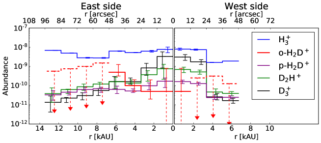
Figure 11: H${}_{3}^{+}$

isotopolog abundances derived from the chemical model constrained by the observations (in particular of ortho-H₂D⁺, which explains why we separately show the two spin states for this species for the sake of clarity).

From N₂H⁺ and N₂D⁺, we can obtain the deuteration ratio, $X$(N₂D⁺)/$X$(N₂H⁺), which is increasing from an upper limit of $\leq$0.05 at large radii to the maximum of 0.34${}^{+0.24}_{-0.15}$ at the center of L 1512. The higher deuteration ratio at the center seems contradictory with the decreasing abundance of ortho-H₂D⁺ toward the center (by a factor of $\lesssim$10). It can be explained if the ortho-H₂D⁺ depletion is due to the further deuteration of H${}_{3}^{+}$. Namely, H₂D⁺ is converted to D₂H⁺ and D${}_{3}^{+}$, which is supported by our chemical modeling best-fit result, $X$(D${}_{3}^{+}$)/$X$(ortho-H₂D⁺) $\approx$ 64 and $X$(D₂H⁺)/$X$(ortho-H₂D⁺) $\approx$ 15 at the innermost layer (Fig. 11). The contrast is higher than toward L 183 (Pagani et al., 2009b, 2013) where D₂H⁺ is comparable to H₂D⁺ in abundance and D${}_{3}^{+}$ less than a factor of 10 higher than H₂D⁺. Moreover, in L 183, the ortho-H₂D⁺ does not show depletion toward the center. This can be linked to the longer timescale of evolution of L 1512 as discussed in Pagani et al. (2013) appendix B, where it is shown that the para-D₂H⁺/ortho-H₂D⁺ is much higher in the slow collapsing case than in the fast collapsing case (the reader should be aware that para-D₂H⁺ is only a small fraction of total D₂H⁺ when comparing the two papers).

Remaining gas-phase CO can react with deuterated H${}_{3}^{+}$ and form DCO⁺ (Pagani et al., 2011), we find that DCO⁺ happens to deplete at $n_{\rm H_{2}}$ of 3 (east) to 7 (west) $\times 10^{4}$ cm^-3, and reaches a depletion factor of 9${}^{+21}_{-3}$ at the center, which is comparable to the factor of $\geq 17$ found in L 183 (Pagani et al., 2012). Like in L 183, DCO⁺ depletes because its parent molecule, CO, freezes out onto dust grains much more than what the growth of H${}_{3}^{+}$ deuteration can compensate for (Pagani et al., 2012). Likewise, N₂H⁺ and N₂D⁺ deplete because of the freeze-out of N₂. CO and N₂ depletion are discussed hereunder.

5.3 CO and N₂ depletion

It is impossible to measure $X$(CO) and $X$(N₂) directly in a dense core. This is because the emission of the low-$J$ transitions of CO (including its isotopologs) usually becomes optically thick even for rarer isotopologs such as C¹⁸O and C¹⁷O, for which the emission is dominated by the envelope and N₂ has no transition detectable in starless cores (Pagani et al., 2012).

In Sect. 4.4, we presented a chemical model to relate the four observed cations (N₂H⁺, N₂D⁺, DCO⁺, and ortho-H₂D⁺) to CO and N₂ in the depleted region to retrieve their abundance profiles. Figure 10 shows the abundance profiles of ¹²CO, C¹⁸O, and N₂. We find that N₂ has a depletion factor of $\sim$200 compared with its maximum values of $3\times 10^{-5}$. For CO isotopologs, ¹²CO has a depletion factor of $\sim$220 compared with its maximum values of $5\times 10^{-5}$. Compared with the standard ¹²CO abundance of 1–$2\times 10^{-4}$ (Pineda et al., 2010), ¹²CO has a depletion factor of $\sim$430–870. C¹⁸O would also have a depletion factor of $\sim$220 compared with its maximum value of $1\times 10^{-7}$ in the outer region since we fix the ¹²C¹⁶O/¹²C¹⁸O ratio of 500, and a factor of $\sim$370 compared to the standard C¹⁸O abundance of $1.7\times 10^{-7}$ (Frerking et al., 1982), which are much larger than the factors of 30 and 25 found by Lippok et al. (2013) and Lee et al. (2003), respectively. Although both studies try to recover volumetric abundances of C¹⁸O and not simply column-density averages, the abundance drop they derive can only be a lower limit because the line from the center is too weak to constrain the models. A factor of 30 already indicates that the contribution of the central part to the total intensity is less than $\sim$10%, which would require a very high signal-to-noise ratio to evaluate and still does not guarantee that the measured variation is not simply due to irregularities in the cloud shape rather than abundance variations (see Pagani et al. 2010a for a similar case).

The abundance of CO and N₂ in starless cores is a matter of long debate (see, e.g., Pagani et al. 2012; Nguyen et al. 2018) since the daughter species of N₂, N₂H⁺, is present at much higher densities than CO itself in starless cores, while CO and N₂ have identical masses and similar sticking coefficients (Bisschop et al., 2006) and their freeze-out rates are thus comparable. For L 1512, ¹²CO and N₂ profiles are similar to each other within their error bars. This is different from the results reported by Pagani et al. (2012) who found a different N₂ profile in L 183, where $X$(N₂) is less than $X$(¹²CO) by about two orders of magnitude at the edge of the starless core. These authors suggest that N₂ might still be forming from atomic N in L 183. In that case, the depletion and production rates of N₂ would partly compensate each other. In contrast with L 183, we find that L 1512 has chemically evolved on a much longer timescale so that N₂ chemical production from atomic N has reached steady state. This could explain the similar depletion profiles. The fact that the CO depletion in L 183 is $\sim$3 times deeper than in L 1512 is mostly due to its peak density being 20 times higher, making collisions with dust grains much more frequent, but the difference is partly compensated by a much longer evolution time in L 1512. The L1512 case is interesting because, by showing that N₂ and CO profiles are identical while N₂H⁺ is tracing the core and not CO, it demonstrates that the N₂/CO problem is not correctly formulated. N₂H⁺ cannot be directly compared to CO because it is a daughter species of N₂ and its abundance therefore also depends on the abundance of H${}_{3}^{+}$. We would need to compare HCO⁺ to N₂H⁺, which is not possible in a simple way. Also, N₂H⁺ is a trace species, typically at the 10^-10 abundance level, at least two orders of magnitude less abundant than CO even depleted by a factor 2000 as in L 183. A correct approach is therefore to compare DCO⁺ and N₂D⁺; in most clouds, it is clearly visible that DCO⁺ is more abundant than N₂D⁺ because its emission is usually as extended as that of N₂H⁺ itself. There is therefore no N₂/CO crisis. However, tracing the abundance of both species in starless cores remains important since it helps the understanding of the chemical evolution of the core.

5.4 Lifetime scale

Figure 9 shows that the chemical solution of each layer meets the observed abundances within $\sim$0.2–2.6 Myr. Since the physical structure is kept constant in our pseudo time-dependent chemical modeling, we see that the chemical process is relatively accelerated in the inner layers compared with the outer layers. Therefore, we underestimate the timescale for the inner layers, which were not very dense at the beginning of contraction. In addition, only the deuteration ratio of N₂D⁺/N₂H⁺ and the abundance of ortho-H₂D⁺ are used to constrain the chemical age, while $X$(DCO⁺) is used to determine the CO abundance. It follows that our result gives a lower limit on the lifetime scale of L 1512 ($\sim$1.43 Myr) that is set by the third western layer, which is the last one in our chemical model to reach the observed N₂D⁺/N₂H⁺ ratio. As a lower limit is required, this value is set at the beginning of the time range of the third western layer as shown on the top right panel (the chemical solutions for the western deuteration ratios) in Fig. 9. We also note that since the third western layer has no ortho-H₂D⁺ detection but only an upper limit on its abundance, the time limit for this layer is the time it takes to reach $X$(N₂D⁺)/$X$(N₂H⁺) under the assumption of $X$(ortho-H₂D⁺) at the maximum of its possible range, that is the fastest time of that layer. Therefore, L 1512 is presumably older than 1.43 Myr. We might ask whether the initial OPR of 3 is warranted. If we set an initial OPR as low as 0.01, we cannot find a good fit for both sides. On the other hand, if we use an OPR of 0.5 as the initial value, as measured in the diffuse medium (Crabtree et al., 2011) toward a few lines of sight, we can only find very marginal fits for both sides and the time remains somewhat above 0.5 Myr. This suggests that the OPR cannot be lower than $\sim$1.

Pagani et al. (2009b) applied the same pseudo time-dependent chemical modeling on L 183 and found the lower limit on L 183 lifetime scale to be 0.15–0.2 Myr. Later, Pagani et al. (2013) conclude that the contraction of L 183 follows the free-fall timescale ($\sim$0.5–0.7 Myr). Namely, L 1512 is older than the L 183 starless core at least by a factor of $\sim$2–3. This is in agreement with our conclusion from Sect. 5.3 that L 1512 may be chemically more evolved than L 183, while physically L 183 has reached a higher density in a shorter time. Consequently, ambipolar diffusion may have slowed down the contraction of L 1512 or even halted it to the present state, while it has had no impact on L 183. This would imply that the magnetic field is stronger in L 1512 than in L 183. This will be the subject of a follow-up study of L 1512.

6 Conclusions

We established the extinction map of L 1512 from deep $JHK_{s}$ and Spitzer/IRAC data. We performed a non-LTE radiative transfer calculation with an onion-shell model to reproduce the observed spectra of L1512. We obtained separately, for the east and west sides, 1D spherically symmetric profiles of the physical parameters and chemical abundances of N₂H⁺, N₂D⁺, DCO⁺, and ortho-H₂D⁺. Afterward, we used a time-dependent chemical model to estimate the lower limit on the lifetime scale of L 1512 by fitting the chemical solutions to the observed abundances. Our chemical model captures the main reactions in the H${}_{3}^{+}$ deuteration fractionation and assumes that heavy species are totally depleted except for CO and N₂, which are partially depleted. Thus, by relating the observed abundances to CO and N₂ in the depleted region, we could also obtain the CO and N₂ profiles and their depletion factors. We summarize our results as follows:

1. We derived the central molecular hydrogen density of $1.1\times 10^{5}$ cm^-3 from the dust extinction measured from NIR and MIR maps and the central kinetic temperature of 7.5$\pm$1 K from N₂H⁺ observations. At such density, gas is thermalized with dust.

2. The depletion factors of N₂H⁺, N₂D⁺, DCO⁺, and ortho-H₂D⁺ are 27${}^{+17}_{-13}$, 4${}^{+2}_{-1}$, 9${}^{+21}_{-3}$, and $\lesssim$10. Compared with N₂H⁺, the smaller N₂D⁺ depletion factor is due to the deuterium fractionation enhanced from a upper limit of $\leq 0.05$ at large radii to 0.34${}^{+0.24}_{-0.15}$ in the center. The depletion of ortho-H₂D⁺ suggests that ortho-H₂D⁺ is further deuterated to D₂H⁺ and D${}_{3}^{+}$.

3. The depletion of N₂H⁺ and N₂D⁺ traces the freezing out of N₂ toward the center of L 1512. We find that N₂ has a depletion factor of $\sim$200 compared to its maximum abundance of $4.7\times 10^{-5}$. Likewise, the depletion of DCO⁺ indicates the freeze-out of CO. We find that ¹²CO and C¹⁸O have a depletion factor of $\sim$220 between internal and external layers. If we compare their minimum abundance to their standard (literature) abundance, we find the depletion factor is about 400 for both isotopologs.

4. The similarity of CO and N₂ profiles suggests that L 1512 may have chemically evolved long enough and in particular that N₂ chemistry has reached its steady state. This could explain that L 1512 has a higher depletion factor of N₂ compared to the denser starless core, L 183.

5. L 1512 is presumably older than 1.4 Myr. We conclude that ambipolar diffusion is the dominant core formation mechanism for this source.

In summary, our results present a precise description of density, temperature, and molecular abundances in a starless core.

Appendix A Spectral line observations

We present spectral line observations other than the main horizontal and vertical cuts and the full C¹⁸O horizontal cut.

Figures 12, 13, 14, 15, and 16 show all the single pointing observations in black lines and models of N₂H⁺ (1–0), N₂H⁺ (3–2), N₂D⁺ (2–1), DCO⁺ (2–1), and ortho-H₂D⁺ (1₁₀–1₁₁) in red lines, respectively. The models are reproduced with our dissymmetric onion-shell model (Sect. 4 and Table 10). The full C¹⁸O (1–0) spectra along the main horizontal cut is shown in Fig. 17, which is an extension of the C¹⁸O spectra in Fig. 8. Since the C¹⁸O emission extending toward the outskirts becomes asymmetric to the core center, we adopt two slab models for reproducing the spectra at $\Delta$Dec $\leq-72$^′′ (west) and $\Delta$Dec $\geq 120$^′′ (east), respectively, instead of the above onion-shell model. To fit the observations in the outskirts, the C¹⁸O abundance of the slab models are fixed to 10^-7 (Sect. 4.4) and $N_{\rm H_{2}}$ is found to be 3.5–5.6$\times 10^{21}$ cm^-2 for the western slab and 0.8–2.6$\times 10^{21}$ cm^-2 for the eastern slab.

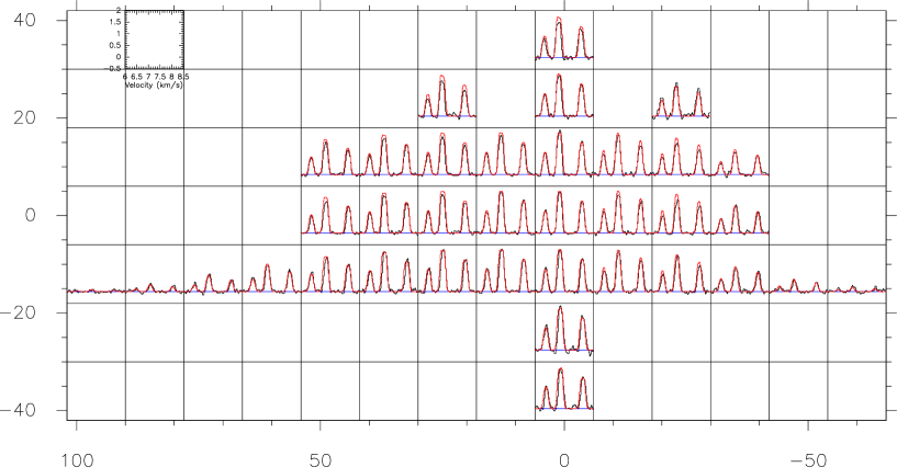
Figure 12: N₂H⁺ (1–0) spectra. The $x$- and $y$-axes of the grid are the RA and Dec offsets with respect to the center of L 1512. Each cell shows the observational spectra as black, the modeled spectra as red, and the baselines as blue. The dimension of $T_{\rm A}^{*}$ and $V_{\rm LSR}$ at each cell are denoted in one of the empty cells. Only the central triplet is shown for clarity.

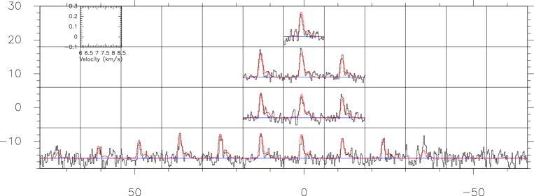
Figure 13: N₂H⁺ (3–2) spectra. Annotations are the same as in Fig. 12.

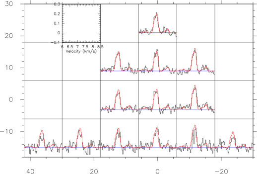
Figure 14: N₂D⁺ (2–1) spectra. Annotations are the same as in Fig. 12.

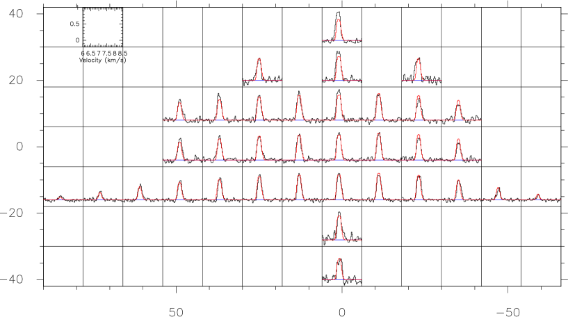
Figure 15: DCO⁺ (2–1) spectra. Annotations are the same as in Fig. 12.

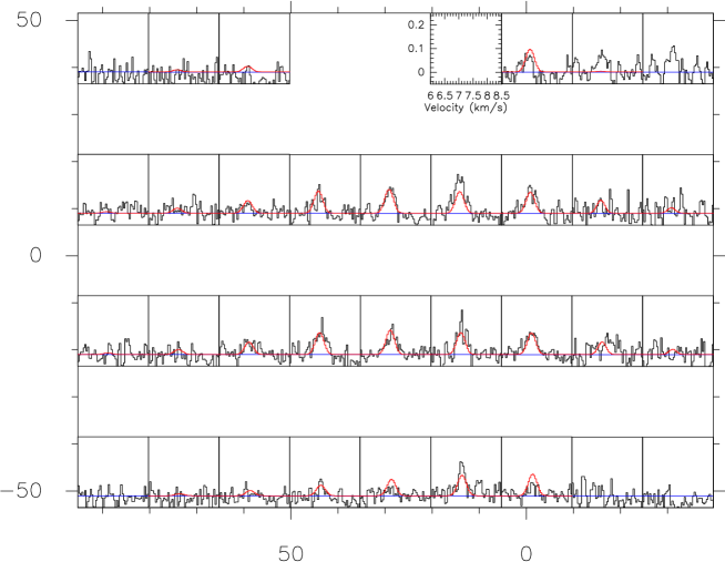
Figure 16: H₂D⁺ (1₁₀–1₁₁) spectra. Annotations are the same as in Fig. 12.

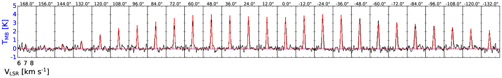
Figure 17: C¹⁸O (1–0) spectra along the main horizontal cut at $\Delta$Dec=$-$12^′′. Annotations are the same as in Fig. 12 except that the emissions are in the $T_{\rm MB}$ scale.

Appendix B N₂D⁺–H₂ collisional rate coefficients

Rate coefficients for the N₂H⁺–H${}_{2}(J=0)$ collisional system have been provided by Lique et al. (2015). Hyperfine-structure-resolved rate coefficients, based on a highly accurate ab initio potential energy surface (PES) (Spielfiedel et al. 2015), were calculated for temperatures ranging from 5 to 70 K. The new rate coefficients were found to be significantly different from the N₂H⁺–He rate coefficients previously published (Daniel et al. 2005).

Recent studies (Dumouchel et al. 2012; Flower & Lique 2015; Dumouchel et al. 2017) have shown that isotopic effects in inelastic collisions can be important, especially for H/D substitution. Hence, we decided to compute actual N₂D⁺–H${}_{2}(J=0)$ rate coefficients.

Within the Born-Oppenheimer approximation, the full electronic ground state potential is identical for N₂H⁺–H₂ and N₂D⁺–H${}_{2}(J=0)$ systems and depends only on the mutual distances of the five atoms involved. Then, we used for the scattering calculations the N₂H⁺–H₂ PES of Spielfiedel et al. (2015) and the “adiabatic-hindered-rotor” treatment, which allows para-H${}_{2}(J=0)$ to be treated as if it were spherical. The major difference between the N₂H⁺–H₂ and N₂D⁺–H${}_{2}(J=0)$ PESs is the position of the center of mass taken for the origin of the Jacobi coordinates. For N₂D⁺–H${}_{2}(J=0)$ calculations, we considered the effect of the displacement of the center of mass.

Since the nitrogen atoms possess a non-zero nuclear spin ($I=1$), the N₂D⁺ rotational energy levels, such as those of N₂H⁺, are split in hyperfine levels, which are characterized by the quantum numbers $J$, $F_{1}$ and $F$. In this case, $F_{1}$ results from the coupling of the rotational level $\@vec{J}$ with $\@vec{I_{1}}$ ($\@vec{F_{1}}=\@vec{J}+\@vec{I_{1}}$, $I_{1}$ being the nuclear spin of the first nitrogen atom) and $F$ results from the coupling of $\@vec{F_{1}}$ with $\@vec{I_{2}}$ ($\@vec{F}=\@vec{F_{1}}+\@vec{I_{2}}$, $I_{2}$ being the nuclear spin of the second nitrogen atom). The D atom also possesses a non-zero nuclear spin. However, in the astronomical observations, the hyperfine structure due to D is not resolved and is then neglected in the calculations.

The hyperfine splitting of the N₂D⁺ energy levels is very small. Considering that the hyperfine levels are degenerate, we simplified the hyperfine scattering problem using recoupling techniques (Faure & Lique 2012). Then, we performed Close-Coupling calculations (Arthurs & Dalgarno 1960) of the pure rotational excitation cross sections (neglecting the hyperfine structure) using the MOLSCAT program (Hutson & Green 1994). The N₂D⁺ energy levels were computed using the rotational constants of Dore et al. (2009). Calculations were carried out for total energies up to 500 cm^-1. Parameters of the integrator were tested and adjusted to ensure a typical precision to within 0.05 Ų for the inelastic cross sections. At each energy, channels with $J$ up to 28 were included in the rotational basis to converge the calculations for all the transitions including N₂D⁺ levels up to $J=7$. Using the recoupling technique, the hyperfine state-resolved cross sections were obtained for all hyperfine levels up to $J=7$.

From the calculated cross sections, we can obtain the corresponding thermal rate coefficients at temperature $T$ by an average over the collision energy ($E_{\rm c}$), i.e.,

$$k_{\rm\alpha\rightarrow\beta}(T) = \left(\frac{8}{\pi\mu k^{3}_{\rm B}T^{3}}\right)^{\frac{1}{2}}$$ (4)

$$\times\int_{0}^{\infty}\sigma_{\rm\alpha\rightarrow\beta}\,E_{\rm c}\,e^{-\frac{E_{\rm c}}{k_{\rm B}T}}\,dE_{\rm c},$$

where $\sigma_{\rm\alpha\to\beta}$ is the cross section from initial level $\alpha$ to final level $\beta$, $\mu$ is the reduced mass of the system, and $k_{\rm B}$ is Boltzmann’s constant.

Using the computational scheme described above, we obtained N₂D⁺–H${}_{2}(J=0)$ rate coefficients for temperatures up to 70 K. The complete set of (de-)excitation rate coefficients with $J,\,J^{\prime}\leq 7$ will be made available through the LAMDA (Schöier et al. 2005) and BASECOL (Dubernet et al. 2013) databases.

Figure 18 presents the temperature variation of the N₂H⁺–H${}_{2}(J=0)$ and N₂D⁺–H${}_{2}(J=0)$ rate coefficients for selected $J=2,F_{1},F\to J^{\prime}=1,F_{1}^{\prime},F^{\prime}$ and $J=3,F_{1},F\to J^{\prime}=2,F_{1}^{\prime},F^{\prime}$ transitions.

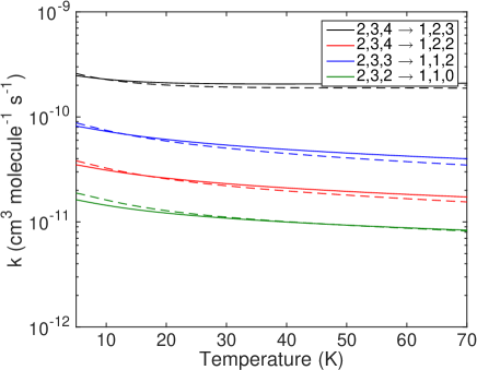
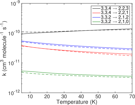
Figure 18: Temperature variation of the hyperfine-resolved N₂H⁺–H${}_{2}(J=0)$ (solid lines) and N₂D⁺–H${}_{2}(J=0)$ (dotted lines) rate coefficients for $J=2,F\to J^{\prime}=1,F^{\prime}$ and $J=3,F\to J^{\prime}=2,F^{\prime}$ transitions.

As is shown, a very good agreement is found between N₂H⁺–H${}_{2}(J=0)$ and N₂D⁺–H${}_{2}(J=0)$ rate coefficients. Both sets of data agree within a few percents over all the temperature range. The largest deviations are seen at a low temperature ($T<10$ K) that characterizes cold molecular clouds. The N₂H⁺ over N₂D⁺ rate coefficients ratio depends on the temperature showing that extrapolation techniques are not suited for the estimation of N₂D⁺ collisional data. The differences are due to both the center-of-mass shift on the interaction potential and the use of isotopolog specific energies of the levels.

Appendix C Best-fit physical and abundance profiles

We present the best-fit quantities with their error ranges for each layer in the onion-shell model from Fig. 8 and Fig. 10 in Table 10.

Table 2: Onion-shell model parameters.

$r$	$n_{\rm H_{2}}$	$T_{\rm kin}$	$X$(N2H+)	$X$(N2D+)	$D_{\rm N_{2}H^{+}}$	$X$(DCO+)	$X$(o-H2D+)	$X$(CO)	$X$(C18O)	$X$(N2)
(kAU)	(cm-3)	(K)
East side
0.00–1.68	1.06(5)	7.5${}_{-2}^{+4}$	3.31${}_{-2.26}^{+3.30}$(-11)	1.13${}_{-0.42}^{+1.13}$(-11)	0.34${}_{-0.27}^{+0.48}$	1.57${}_{-0.32}^{+6.31}$(-11)	5.00${}_{-\inf}^{+74.24}$(-11)	3.16${}_{-2.16}^{+6.84}$(-7)	6.32(-10)	1.45${}_{-0.84}^{+2.03}$(-7)
1.68–3.36	8.43(4)	8.2${}_{-2}^{+1}$	9.20${}_{-3.40}^{+2.38}$(-11)	1.13${}_{-0.42}^{+1.13}$(-11)	0.12${}_{-0.06}^{+0.13}$	6.40${}_{-1.32}^{+1.66}$(-11)	5.00${}_{-3.00}^{+14.91}$(-11)	5.19${}_{-2.21}^{+3.83}$(-6)	1.04${}_{-0.38}^{+2.25}$(-8)	3.77${}_{-0.91}^{+1.20}$(-7)
3.36–5.04	6.00(4)	8.5${}_{-2}^{+1}$	4.36${}_{-0.90}^{+1.13}$(-10)	2.20${}_{-0.45}^{+0.57}$(-11)	0.05${}_{-0.01}^{+0.02}$	8.72${}_{-1.79}^{+2.26}$(-11)	1.00${}_{-0.50}^{+0.99}$(-10)	1.00${}_{-0.50}^{+0.99}$(-5)	2.00${}_{-0.74}^{+1.17}$(-8)	3.51${}_{-1.44}^{+2.45}$(-6)
5.04–6.72	4.21(4)	9.2${}_{-4}^{+1}$	9.06${}_{-5.46}^{+2.35}$(-10)	5.01${}_{-1.03}^{+1.30}$(-11)	0.06${}_{-0.04}^{+0.02}$	1.03${}_{-0.21}^{+0.27}$(-10)	5.00${}_{-1.85}^{+7.56}$(-10)	9.16${}_{-2.21}^{+2.92}$(-6)	1.83${}_{-0.68}^{+3.96}$(-8)	6.47${}_{-1.56}^{+2.06}$(-6)
6.72–8.40	3.01(4)	9.3${}_{-2}^{+1}$	1.09${}_{-0.40}^{+0.28}$(-9)	¡5.44(-11)	¡0.05	1.54${}_{-0.32}^{+0.90}$(-10)	¡1.50(-9)	3.16${}_{-2.16}^{+6.84}$(-5)	7.74${}_{-1.59}^{+7.71}$(-8)	2.65${}_{-1.95}^{+7.41}$(-5)
8.40–10.08	2.23(4)	10.4${}_{-1}^{+1}$	9.06${}_{-1.86}^{+2.35}$(-10)	¡4.53(-11)	¡0.05	1.67${}_{-0.34}^{+0.97}$(-10)	¡9.98(-10)	5.00${}_{-2.49}^{+4.98}$(-5)	1.00${}_{-0.21}^{+1.00}$(-7)	3.00${}_{-2.01}^{+6.06}$(-5)
10.08–11.76	1.70(4)	10.5${}_{-1}^{+4}$	4.21${}_{-0.87}^{+4.20}$(-10)	¡2.11(-11)	¡0.05	8.48${}_{-1.74}^{+2.19}$(-11)	¡7.54(-10)	5.00(-5)	1.00${}_{-0.21}^{+1.00}$(-7)	1.06${}_{-0.31}^{+0.44}$(-5)
11.76–13.44	1.33(4)	11.2${}_{-3}^{+6}$	1.30${}_{-0.27}^{+1.97}$(-10)	¡6.52(-12)	¡0.05	3.12${}_{-0.64}^{+6.75}$(-11)	¡5.65(-10)	5.00(-5)	1.00${}_{-0.21}^{+1.51}$(-7)	3.54${}_{-1.03}^{+1.46}$(-6)
13.44–15.12	1.07(4)	12.3${}_{-6}^{+6}$	1.85${}_{-0.93}^{+12.88}$(-11)	¡9.28(-13)	¡0.05	–	–	–	1.00${}_{-0.21}^{+0.26}$(-7)	–
West side
0.00–1.68	1.10(5)	7.5${}_{-1}^{+1}$	3.31${}_{-0.68}^{+0.86}$(-11)	1.13${}_{-0.42}^{+0.29}$(-11)	0.34${}_{-0.14}^{+0.13}$	1.57${}_{-0.78}^{+0.41}$(-11)	5.00${}_{-\inf}^{+74.24}$(-11)	1.45${}_{-0.76}^{+1.58}$(-7)	2.90(-10)	1.64${}_{-0.51}^{+0.73}$(-7)
1.68–3.36	1.00(5)	7.5${}_{-2}^{+1}$	1.52${}_{-0.31}^{+0.39}$(-10)	3.16${}_{-0.65}^{+0.82}$(-11)	0.21${}_{-0.06}^{+0.08}$	5.83${}_{-1.20}^{+1.51}$(-11)	¡2.52(-10)	1.18${}_{-0.49}^{+0.83}$(-6)	2.37${}_{-1.62}^{+7.05}$(-9)	8.03${}_{-1.94}^{+2.56}$(-7)
3.36–5.04	7.60(4)	8.0${}_{-2}^{+1}$	6.75${}_{-1.39}^{+1.75}$(-10)	3.16${}_{-0.65}^{+0.82}$(-11)	0.05${}_{-0.01}^{+0.02}$	1.00${}_{-0.21}^{+0.26}$(-10)	¡3.15(-10)	2.51${}_{-1.80}^{+63.95}$(-5)	5.02${}_{-1.03}^{+1.30}$(-8)	1.78${}_{-1.43}^{+7.33}$(-5)
5.04–6.72	4.86(4)	8.0${}_{-1}^{+1}$	2.68${}_{-0.55}^{+0.69}$(-10)	¡1.26(-11)	¡0.05	1.27${}_{-0.26}^{+0.33}$(-10)	¡1.26(-10)	5.00(-5)	1.00${}_{-0.21}^{+0.26}$(-7)	8.66${}_{-1.12}^{+1.28}$(-6)
6.72–8.40	2.94(4)	9.0${}_{-2}^{+2}$	1.64${}_{-0.99}^{+0.42}$(-10)	¡7.70(-12)	¡0.05	8.73${}_{-1.80}^{+2.26}$(-11)	–	–	1.00${}_{-0.21}^{+0.26}$(-7)	–
8.40–10.08	1.81(4)	9.5${}_{-2}^{+6}$	5.97${}_{-1.23}^{+3.49}$(-11)	¡2.80(-12)	¡0.05	7.02${}_{-1.44}^{+1.82}$(-11)	–	–	1.00${}_{-0.37}^{+0.58}$(-7)	–