Asymptotics of the principal eigenvalue for a linear time-periodic parabolic operator I: Large advection

Abstract.

We investigate the effect of large advection on the principal eigenvalues of linear time-periodic parabolic operators with zero Neumann boundary conditions. Various asymptotic behaviors of the principal eigenvalues, when advection coefficient approaches infinity, are established, where spatial or temporal degeneracy could occur in the advection term. Our findings substantially improve the results in [43] for parabolic operators and also extend the existing results in [9, 45] for elliptic operators.

1. Introduction

In this paper, we consider the following linear eigenvalue problem for time-periodic parabolic operators in one-dimensional space:

(1.1) $$\left\{\begin{array}[]{ll}\vskip 6.0pt plus 2.0pt minus 2.0pt\partial_{t}\varphi-D\partial_{xx}\varphi-\alpha\partial_{x}m\partial_{x}\varphi+V\varphi=\lambda\varphi&{\text{in}}\,\,(0,1)\times[0,T],\\ \vskip 6.0pt plus 2.0pt minus 2.0pt\partial_{x}\varphi(0,t)=\partial_{x}\varphi(1,t)=0&{\text{on}}\,\,[0,T],\\ \varphi(x,0)=\varphi(x,T)&\text{on}\,\,(0,1),\end{array}\right.$$

where the positive parameters $D$ and $\alpha$ are diffusion and advection rates, respectively. The functions $m\in C^{2,0}([0,1]\times\mathbb{R})$ and $V\in C([0,1]\times\mathbb{R})$ are assumed to be periodic in $t$ with a common period $T$. It is well known [18, Proposition 7.2] that problem (1.1) admits a principal eigenvalue $\lambda(\alpha)$, which is real and simple, and the corresponding eigenfunction can be chosen to be positive. Furthermore, $\lambda(\alpha)<\mathrm{Re}(\lambda)$ holds for any other eigenvalue $\lambda$ of (1.1).

The goal of this paper is to determine the limit of $\lambda(\alpha)$ as $\alpha\to\infty$. The asymptotic behavior of the principal eigenvalue for (1.1) as $D\to 0$ will be considered in [31].

1.1. Background

Besides its own mathematical interest, the asymptotic behavior of the principal eigenvalue of (1.1) for large advection rate $\alpha$ is also motivated by its applications to biological problems, including: (i) the phytoplankton growth with periodic light intensity; (ii) the persistence and competition of species in rivers with spatio-temporally varying drift; (iii) the competition of species along the gradient of spatial-temporally varying resources; (iv) the spreading of epidemic diseases in time-periodic advective environments, among others. We refer to [3, 11, 24, 25] and references therein for further discussions. In the following we highlight two potential applications of our results:

Persistence for a single species. The population dynamics of a single species, subject to spatio-temporally varying environmental drifts, can be modeled as

(1.2) $$\begin{cases}\begin{array}[]{ll}\vskip 3.0pt plus 1.0pt minus 1.0pt\partial_{t}U=\partial_{x}\left(D\partial_{x}U-\alpha U\partial_{x}\tilde{m}\right)+Uf(x,t,U)&{\text{in}}\,\,(0,1)\times(0,\infty),\\ D\partial_{x}U-\alpha U\partial_{x}\tilde{m}=0&{\text{on}}\,\,\{0,1\}\times(0,\infty),\end{array}\end{cases}$$

where $\tilde{m}$ and $f$ are assumed to be $T$-periodic and $U$ denotes the density of the population; see [3, 18, 40] for more details. For instance, model (1.2) can describe the phytoplankton growth in light limited water columns [13, 14, 20, 35, 43, 44, 47] or hydrobiological species in rivers [48]. An important biological issue is how drift affects the population dynamics of (1.2) [41]. Mathematically, the persistence of the single species in (1.2) is equivalent to the instability of trivial equilibrium $U\equiv 0$ [3], which is in turn determined by the sign of the principal eigenvalue $\lambda(\alpha)$ of the linear problem (1.1) with $V=-f(x,T-t,0)$ and $m=\tilde{m}(x,T-t)$, by considering the corresponding adjoint operator. If the environment is spatio-temporally varying, i.e. $\partial_{x}\tilde{m}$ and $f$ depend on $x$ and $t$ non-trivially (e.g. phytoplankton population drifts up and down in the water column periodically in time, and the light intensity at the water surface also varies periodically in time), then determining the sign of $\lambda(\alpha)$ becomes a challenging issue, and standard spectral theory is often not sufficient.

When $m$ and $f$ are independent of time, the high-dimensional version of (1.2) was initially proposed in [2], where it is assumed that the species may have the tendency to move upward along the resource gradient. They investigated whether such directed movement could help promote the persistence of a single species. A related question is to determine the optimal distribution of resources for a single species to survive: When $\alpha=0$, it was shown in [39] that, under a regularity assumption, the optimal distribution $m^{*}$ that maximizes the total biomass of a single species is of the “bang-bang” type, i.e. $m^{*}=\chi_{E}$ for some measurable set $E$, where $\chi_{E}$ denotes the characteristic function of $E$; when $\alpha\neq 0$, by studying the minimization of the principal eigenvalue of problem (1.1) with proper constraint on $m$, the optimal distribution was fully determined in [8] for the one-dimensional case; see also [36] for the recent progress on the higher dimensional case. We also refer to [17] for optimization problems on the principal eigenvalues for elliptic operators with drift. It will be of interest to investigate the principal eigenvalue of problem (1.1) under weaker regularity of $m$ and $V$, e.g. when $m$ and/or $V$ are of the form $\chi_{E}$. Such questions are even not well understood for time-independent $m$ and $V$.

Competition for two species. The two competing species in time-periodic and advective environment can be modeled by the following reaction-diffusion-advection system:

(1.3) $$\left\{\begin{array}[]{ll}\vskip 6.0pt plus 2.0pt minus 2.0pt\partial_{t}U_{1}=\partial_{x}\left(D\partial_{x}U_{1}-\alpha_{1}U_{1}\partial_{x}m\right)+U_{1}f(x,t,U_{1},U_{2})&\text{in }(0,1)\times(0,\infty),\\ \vskip 6.0pt plus 2.0pt minus 2.0pt\partial_{t}U_{2}=\partial_{x}\left(D\partial_{x}U_{2}-\alpha_{2}U_{2}\partial_{x}m\right)+U_{2}g(x,t,U_{1},U_{2})&\text{in }(0,1)\times(0,\infty),\\ D\partial_{x}U_{1}-\alpha_{1}U_{1}\partial_{x}m=D\partial_{x}U_{2}-\alpha_{2}U_{2}\partial_{x}m=0&\text{on }\{0,1\}\times(0,\infty),\end{array}\right.$$

where $m$, $f$ and $g$ are $T$-periodic functions, and $U_{1},U_{2}$ are the population densities of two species. When the coefficients are time independent, model (1.3) was first proposed in [6] to study whether or not the advection along the resource gradient can confer competition advantage; see also [1, 7]. When $\partial_{x}m$ is a positive constant, (1.3) reduces to the river model studied in [26, 27, 32, 33, 34, 49, 51], where the evolution of biased movement was considered. Since (1.3) generates a monotone dynamical system [18], the dynamics of (1.3) is determined to a large extent by its steady periodic states and their stability properties. For example, the existence and stability of coexistence states for (1.3) follow from the instability of the two semi-trivial states and theory for monotone systems [18, 19]. The stability of semi-trivial periodic state turns out to be determined by the sign of the principal eigenvalue of the linear problem (1.1) by considering the linearization at this semi-trivial state. Therefore, the qualitative properties of principal eigenvalue with respect to $\alpha$ plays a pivotal role in analyzing the impact of the advection on the outcome of the competition in time-periodic environments.

1.2. Previous work

Let $\lambda(\alpha)$ denote the principal eigenvalue of (1.1). Observe that when $V$ depends on the time variable alone, i.e. $V(x,t)=V(t)$, there holds $\lambda(\alpha)\equiv\frac{1}{T}\int_{0}^{T}V\left(s\right)\mathrm{d}s$ for all $\alpha$. When $V$ and $\partial_{x}m$ depend on the space variable alone, i.e. $V(x,t)=V(x)$ and $\partial_{x}m(x,t)=m^{\prime}(x)$, (1.1) reduces to the following elliptic eigenvalue problem:

(1.4) $$\left\{\begin{array}[]{ll}\vskip 6.0pt plus 2.0pt minus 2.0pt-D\varphi^{\prime\prime}-\alpha m^{\prime}(x)\varphi^{\prime}+V(x)\varphi=\lambda\varphi&\text{in}\,\,(0,1),\\ \varphi^{\prime}(0)=\varphi^{\prime}(1)=0.\end{array}\right.$$

For this simple-looking ODE eigenvalue problem, identifying the sign of $\lambda(\alpha)$ is not yet trivial. In the recent works [9, 10, 28, 42, 45], the asymptotic behaviors of the principal eigenvalue for large $\alpha$ or small $D$ has been extensively studied for (1.4) and its high dimensional version.

However, when $V$ or/and $\partial_{x}m$ depend both on the spatio-temporal variables, much less has been known about the asymptotic behaviors of $\lambda(\alpha)$, partly due to the lack of variational structure for problem (1.1). One may refer to [12, 15, 18, 21, 30, 37, 38, 43], among others, for some progresses in this direction. In particular, in the case of $V(x,t)=\mu v(x,t)$ for some $T$-periodic function $v\geq 0,\not\equiv 0$, the authors in [12, 15] studied the limiting behaviors of the principal eigenvalue as $\mu\to\infty$ when the weight function $v$ may be spatio-temporally degenerate (i.e. vanishes). In [30], we established some monotonicity and asymptotic behaviors of $\lambda(\alpha)$ with respect to time period $T$. If the advection is monotone in space $x$, i.e. $|\partial_{x}m|>0$, the limiting behaviors of the principal eigenvalue for large $\alpha$ or small $D$ were investigated in [43]. However, the asymptotics of $\lambda(\alpha)$ remain open for general advection.

We also refer to [4, 5, 22, 29] for some applications of the principal eigenvalues to the evolution of dispersal in time-periodic environments.

1.3. Main results

Throughout this paper, we set $D=1$ in (1.1). To state the main results, we introduce some notations for advection $m$.

• A spatially interior critical point of $m$ is a point $(x_{*},t_{*})\in(0,1)\times[0,T]$ such that $\partial_{x}m(x_{*},t_{*})=0$, and it is called nondegenerate if $\partial_{xx}m(x_{*},t_{*})\neq 0$.

• The boundary point $(x_{*},t_{*})\in\{0,1\}\times[0,T]$ is always called spatially critical, and it is called nondegenerate if either $\partial_{x}m(x_{*},t_{*})\neq 0$ or $\partial_{xx}m(x_{*},t_{*})\neq 0$.

• A point of spatially local maximum of $m$ is a point $(x_{*},t_{*})\in[0,1]\times[0,T]$ that satisfies $m(x_{*},t_{*})\geq m(x,t_{*})$ in a small neighborhood of $x_{*}$ with respect to $[0,1]$.

Our first main result concerns the nondegenerate advection.

Theorem 1.1.

Suppose that all spatially critical points of $m$ are nondegenerate. Assume $\{(\kappa_{i}(t),t):t\in[0,T],1\leq i\leq N\}$ with $\kappa_{i}\in C^{1}([0,T])$ is the set of spatially local maximum points of $m$. Let $\lambda(\alpha)$ be the principal eigenvalue of (1.1). Then

(1.5) $$\lim_{\alpha\rightarrow\infty}\lambda(\alpha)=\min_{1\leq i\leq N}\left\{\frac{1}{T}\int_{0}^{T}V\left(\kappa_{i}(s),s\right)\mathrm{d}s\right\}.$$

If the function $m$ admits finitely many isolated maxima for every $t$, we conjecture that Theorem 1.1 remains true for the higher dimensional case. Determining the asymptotic profile of the principal eigenfunction is also an interesting question. We suspect that the corresponding principal eigenfunction will concentrate on some of these curves $x=\kappa_{i}(t)$ as $\alpha\to\infty$.

Remark 1.1.

When $V$ and $m$ are independent of time, Theorem 1.1 is reduced to [9, Theorem 1.1] for elliptic problem (1.4) in one-dimensional case. If $\partial_{x}m>0$ (resp. $\partial_{x}m<0$) in $[0,1]\times[0,T]$, it follows from Theorem 1.1 that

$$\lim\limits_{\alpha\rightarrow\infty}\lambda(\alpha)=\frac{1}{T}\int_{0}^{T}V\left(1,s\right)\mathrm{d}s\ \qquad(\text{resp.}\ \lim\limits_{\alpha\rightarrow\infty}\lambda(\alpha)=\frac{1}{T}\int_{0}^{T}V\left(0,s\right)\mathrm{d}s),$$

which was first established in [43, Theorem 1.1].

Our next result concerns the situation when the advection $m$ can be spatially degenerate, e.g. $m(x,t)$ is constant in an interval for each $t\in[0,T]$. We first introduce some notations.

Let $0\leq\underline{\kappa}(t)<\overline{\kappa}(t)\leq 1$ be two continuous functions defined on $[0,T]$ and $p,q\in\{\mathcal{N},\mathcal{D}\}$. Denote by $\lambda^{pq}\big{(}(\underline{\kappa},\overline{\kappa})\big{)}$ the principal eigenvalue of the problem

(1.6) $$\begin{cases}\begin{array}[]{ll}\partial_{t}\psi-\partial_{xx}\psi+V(x,t)\psi=\lambda\psi,&x\in(\underline{\kappa}(t),\,\overline{\kappa}(t)),\ t\in[0,T],\\ \left(\ell_{1}\psi+(1-\ell_{1})\partial_{x}\psi\right)(\underline{\kappa}(t),t)=0,&t\in\left[0,T\right],\\ \left(\ell_{2}\psi+(1-\ell_{2})\partial_{x}\psi\right)(\overline{\kappa}(t),t)=0,&t\in\left[0,T\right],\\ \psi(x,0)=\psi(x,T),&x\in(\underline{\kappa}(0),\overline{\kappa}(0)),\end{array}\end{cases}$$

where

$$\ell_{1}=\left\{\begin{array}[]{ll}0,&\text{if}~{}~{}p=\mathcal{N},\\ 1,&\text{if}~{}~{}p=\mathcal{D},\end{array}\right.\text{ and }\,\,\ell_{2}=\left\{\begin{array}[]{ll}0,&\text{if}~{}~{}q=\mathcal{N},\\ 1,&\text{if}~{}~{}q=\mathcal{D}.\end{array}\right.$$

The letters $\mathcal{N}$ and $\mathcal{D}$ represent the zero Neumann and Dirichlet boundary conditions, respectively. The existence of $\lambda^{pq}\big{(}(\underline{\kappa},\overline{\kappa})\big{)}$ can be guaranteed by the Krein-Rutman theorem [23]; see also [18, Proposition 7.2].

Given $\kappa_{i}\in C^{1}([0,T])$, $i=0,1,\ldots,N+1$, such that

(1.7) $$0=\kappa_{0}(t)<\kappa_{1}(t)<\ldots<\kappa_{N}(t)<\kappa_{N+1}(t)=1\quad\text{for all }\,\,t\in[0,T],$$

we denote

• $\mathbf{A}=\big{\{}0\leq i\leq N:\ \ \partial_{x}m(x,t)<0\ \ \text{if }\,\,x\in(\kappa_{i}(t),\kappa_{i+1}(t))\big{\}};$

• $\mathbf{B}=\big{\{}0\leq i\leq N:\ \ \partial_{x}m(x,t)=0\ \,\text{if }\,\,x\in[\kappa_{i}(t),\kappa_{i+1}(t)]\big{\}};$

• $\mathbf{C}=\big{\{}0\leq i\leq N:\ \ \partial_{x}m(x,t)>0\ \,\text{if }\,\,x\in(\kappa_{i}(t),\kappa_{i+1}(t))\big{\}}$.

Our second result can be stated as follows.

Theorem 1.2.

Let $\{\kappa_{i}(t)\}_{0\leq i\leq N+1}$ be functions of class $C^{1}$ satisfying (1.7) and $\partial_{x}m(\kappa_{i}(t),t)=0$ for all $t\in[0,T]$ and $1\leq i\leq N$. Assume that $\{0,1,\ldots,N\}=\mathbf{A}\cup\mathbf{B}\cup\mathbf{C}$ and that for any $0\leq i\leq N-1$, $(i,i+1)\not\in\mathbf{A}^{2}\cup\mathbf{B}^{2}\cup\mathbf{C}^{2}$.

Define $\mathbf{E}(\mathcal{N},\mathcal{N}),\mathbf{E}(\mathcal{N},\mathcal{D}),\mathbf{E}(\mathcal{D},\mathcal{N}),\mathbf{E}(\mathcal{D},\mathcal{D})\subset\{0,1,\ldots,N\}$ by setting

$$i\in\mathbf{E}(\mathcal{N},\mathcal{N})\Leftrightarrow\begin{cases}i-1\in\mathbf{C},\,\,i\in\mathbf{B},\,\,i+1\in\mathbf{A}&\text{if }1\leq i\leq N,\\ 0\in\mathbf{B},\,\,1\in\mathbf{A}&\text{if }i=0,\\ N-1\in\mathbf{C},\,\,N\in\mathbf{B}&\text{if }i=N;\\ \end{cases}$$

$$i\in\mathbf{E}(\mathcal{N},\mathcal{D})\Leftrightarrow\begin{cases}i-1\in\mathbf{C},\,\,i\in\mathbf{B},\,\,i+1\in\mathbf{C}&\text{if }1\leq i\leq N,\\ 0\in\mathbf{B},\,\,1\in\mathbf{C}&\text{if }i=0;\\ \end{cases}$$

$$i\in\mathbf{E}(\mathcal{D},\mathcal{N})\Leftrightarrow\begin{cases}i-1\in\mathbf{A},\,\,i\in\mathbf{B},\,\,i+1\in\mathbf{A}&\text{if }1\leq i\leq N,\\ N-1\in\mathbf{A},\,\,N\in\mathbf{B}&\text{if }i=N;\\ \end{cases}$$

$$i\in\mathbf{E}(\mathcal{D},\mathcal{D})\Leftrightarrow i-1\in\mathbf{A},\,\,i\in\mathbf{B},\,\,i+1\in\mathbf{C},\text{ and }1\leq i\leq N.\quad$$

Moreover, define the set $\mathbf{E}\subset\{0,1,\ldots,N+1\}$ by setting

$$i\in\mathbf{E}\Leftrightarrow\begin{cases}i-1\in\mathbf{C},\,\,i\in\mathbf{A},&\text{if }1\leq i\leq N,\\ 0\in\mathbf{A},&\text{if }i=0,\\ N\in\mathbf{C}&\text{if }i=N+1.\end{cases}$$

Let $\lambda(\alpha)$ be the principal eigenvalue of (1.1). Then

(1.8) $$\begin{split}\lim_{\alpha\rightarrow\infty}\lambda(\alpha)=\min\Bigg{\{}&\min_{i\in\mathbf{E}}\left[\frac{1}{T}\int_{0}^{T}V(\kappa_{i}(s),s)\mathrm{d}s\right],\ \ \min_{i\in\mathbf{E}(\mathcal{N},\mathcal{N})}\lambda^{\mathcal{N}\mathcal{N}}_{i},\\ &\min_{i\in\mathbf{E}(\mathcal{N},\mathcal{D})}\lambda^{\mathcal{N}\mathcal{D}}_{i},\ \ \min_{i\in\mathbf{E}(\mathcal{D},\mathcal{N})}\lambda^{\mathcal{D}\mathcal{N}}_{i},\ \ \min_{i\in\mathbf{E}(\mathcal{D},\mathcal{D})}\lambda^{\mathcal{D}\mathcal{D}}_{i}\Bigg{\}},\end{split}$$

where $\lambda^{pq}_{i}=\lambda^{pq}\big{(}(\kappa_{i},\kappa_{i+1})\big{)}$ for $p,q\in\{\mathcal{N},\mathcal{D}\}$.

Remark 1.2.

If $m$ and $V$ are both independent of time, Theorem 1.2 is reduced to [45, Theorem 1.2] for the elliptic eigenvalue problem (1.4). However, the techniques used to prove Theorem 1.2 are rather different from those in [45], due to the lack of variational characterization for the principal eigenvalue of time-dependent problem (1.1).

Remark 1.3.

When $\mathbf{B}=\emptyset$, i.e. there is no spatial degeneracy in advection, $\mathbf{E}(\mathcal{N},\mathcal{N})=\mathbf{E}(\mathcal{N},\mathcal{D})=\mathbf{E}(\mathcal{D},\mathcal{N})=\mathbf{E}(\mathcal{D},\mathcal{D})=\emptyset$ and Theorem 1.2 is a slightly stronger version of Theorem 1.1 without the nondegeneracy assumption on the spatial critical points of $m$. See Remark 3.1 for two examples. When $\mathbf{B}\neq\emptyset$, if we let the strip $(\kappa_{i}(t),\,\kappa_{i+1}(t))$ shrinks to some curve $\tilde{\kappa}_{i}(t)$ for every $i\in\mathbf{B}$, then

$$\lambda^{\mathcal{D}\mathcal{D}}\big{(}(\kappa_{i},\kappa_{i+1})\big{)}\to\infty,\ \ \lambda^{\mathcal{D}\mathcal{N}}\big{(}(\kappa_{i},\kappa_{i+1})\big{)}\to\infty,\ \ \lambda^{\mathcal{N}\mathcal{D}}\big{(}(\kappa_{i},\kappa_{i+1})\big{)}\to\infty,$$

$$\lambda^{\mathcal{N}\mathcal{N}}\big{(}(\kappa_{i},\kappa_{i+1})\big{)}\to\frac{1}{T}\int_{0}^{T}V(\tilde{\kappa}_{i}(s),s)\,\mathrm{d}s.$$

Hence, (1.8) is reduced to (1.5), i.e. Theorem 1.2 coincides with Theorem 1.1.

Remark 1.4.

We further illustrate Theorem 1.2 by the special case

(1.9) $$m(x,t)=m_{1}(x)m_{2}(t),$$

where $m_{2}\in C([0,T])$ is $T$-periodic and $m_{1}\in C^{2}([0,1])$. In the context of Theorem 1.2, assume that $m_{2}>0$ on $[0,T]$ and the graph of $m_{1}$ is given as in Fig. 1 with the set of critical points $\{\kappa_{i}:0\leq i\leq 10\}$. Then $\mathbf{A}=\{0,4,6\}$, $\mathbf{B}=\{2,5,7,9\}$, and $\mathbf{C}=\{1,3,8\}$. Using the notations in Theorem 1.2, $\mathbf{E}=\{0,4\}$, $\mathbf{E}(\mathcal{N},\mathcal{N})=\{9\}$, $\mathbf{E}(\mathcal{N},\mathcal{D})=\{2\}$, $\mathbf{E}(\mathcal{D},\mathcal{N})=\{5\}$, and $\mathbf{E}(\mathcal{D},\mathcal{D})=\{7\}$. Then Theorem 1.2 yields

$$\begin{split}\lim_{\alpha\rightarrow\infty}\lambda(\alpha)=\min\Bigg{\{}&\frac{1}{T}\int_{0}^{T}V(0,s)\mathrm{d}s,\ \ \frac{1}{T}\int_{0}^{T}V(\kappa_{4},s)\mathrm{d}s,\ \ \lambda^{\mathcal{N}\mathcal{N}}\big{(}(\kappa_{9},\kappa_{10})\big{)},\\ &\lambda^{\mathcal{N}\mathcal{D}}\big{(}(\kappa_{2},\kappa_{3})\big{)},\ \ \lambda^{\mathcal{D}\mathcal{N}}\big{(}(\kappa_{5},\kappa_{6})\big{)},\ \ \lambda^{\mathcal{D}\mathcal{D}}\big{(}(\kappa_{7},\kappa_{8})\big{)}\Bigg{\}}.\end{split}$$

We also refer to Propositions 4.1 and 4.2 for further details.

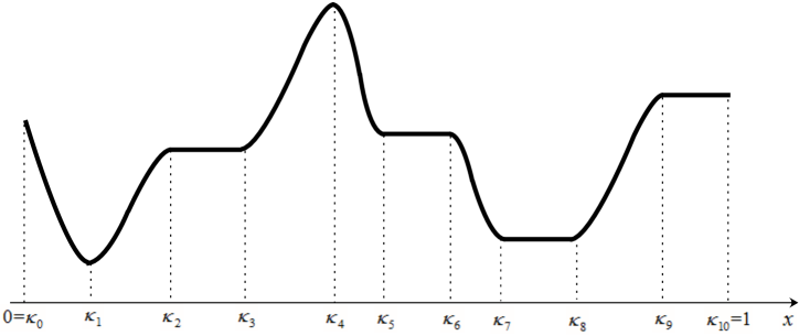
Figure 1. An example of $m_{1}(x)$ with degenerate critical points in Remark 1.4, where $\kappa_{i}$ ($0\leq i\leq 10$) denotes its critical point.

Our next result concerns the effect of temporally degenerate advection on the limit of $\lambda(\alpha)$ as $\alpha\rightarrow\infty$. To emphasize the ideas of our proof and also make the presentation of our result clearer, assume $\partial_{x}m(x,t)=b(t)$ for some $T$-periodic function $b$, where $b$ allows to vanish somewhere and is referred as the temporal degeneracy. Then problem (1.1) becomes

(1.10) $$\begin{cases}\begin{array}[]{ll}\vskip 3.0pt plus 1.0pt minus 1.0pt\partial_{t}\varphi-\partial_{xx}\varphi-\alpha b(t)\partial_{x}\varphi+V(x,t)\varphi=\lambda\varphi&\text{in}\,\,(0,1)\times[0,T],\\ \vskip 3.0pt plus 1.0pt minus 1.0pt\partial_{x}\varphi(0,t)=\partial_{x}\varphi(1,t)=0&{\text{on}}\,\,[0,T],\\ \varphi(x,0)=\varphi(x,T)&{\text{on}}\,\,(0,1).\end{array}\end{cases}$$

Hereafter, for any $\phi\in C([0,1]\times\mathbb{R})$, we use the notations $\phi(\cdot,t^{+})$ and $\phi(\cdot,t^{-})$ to represent the right and left limit of $\phi$ at time $t$ respectively; similarly, the notations $\phi(x^{+},\cdot)$ and $\phi(x^{-},\cdot)$ mean the right and left limit at spatial location $x$.

Theorem 1.3.

Given any sequence $\{t_{i}\}_{0\leq i\leq N+1}$ with $0=t_{0}<t_{1}<\ldots<t_{N+1}=T$, denote

$$\begin{array}[]{c}\mathbb{A}=\big{\{}0\leq i\leq N:\ \,b(t)<0\,\text{ in }(t_{i},t_{i+1})\big{\}},\\ \mathbb{B}=\big{\{}0\leq i\leq N:\ \,b(t)\equiv 0\,\text{ on }[t_{i},t_{i+1}]\big{\}},\\ \mathbb{C}=\big{\{}0\leq i\leq N:\ \,b(t)>0\,\text{ in }(t_{i},t_{i+1})\big{\}}.\end{array}$$

Assume $\mathbb{A}\cup\mathbb{B}\cup\mathbb{C}=\{0,\ldots,N\}$. Let $\lambda(\alpha)$ be the principal eigenvalue of (1.10). Then $\lambda(\alpha)\to\lambda_{\infty}$ as $\alpha\rightarrow\infty$, where $\lambda_{\infty}$ is the principal eigenvalue of the problem

(1.11) $$\begin{cases}\left.\begin{array}[]{ll}\vskip 3.0pt plus 1.0pt minus 1.0pt\partial_{t}\psi+V(0,t)\psi=\lambda\psi&{\text{in}}\,\,(0,1)\times\left(t_{i},t_{i+1}\right],\\ \psi(x,t_{i}^{+})\equiv\psi(0,t_{i}^{-})&{\text{on}}\,\,(0,1),\\ \end{array}\right\}\ i\in\mathbb{A}\\ \left.\begin{array}[]{ll}\vskip 3.0pt plus 1.0pt minus 1.0pt\partial_{t}\psi-\partial_{xx}\psi+V(x,t)\psi=\lambda\psi&{\text{in}}\,\,(0,1)\times\left(t_{i},t_{i+1}\right],\\ \psi(x,t_{i}^{+})=\psi(x,t_{i}^{-})&{\text{on}}\,\,(0,1),\\ \end{array}\right\}\ i\in\mathbb{B}\\ \left.\begin{array}[]{ll}\vskip 3.0pt plus 1.0pt minus 1.0pt\partial_{t}\psi+V(1,t)\psi=\lambda\psi&{\text{in}}\,\,(0,1)\times\left(t_{i},t_{i+1}\right],\\ \psi(x,t_{i}^{+})\equiv\psi(1,t_{i}^{-})&{\text{on}}\,\,(0,1),\\ \end{array}\right\}\ i\in\mathbb{C}\\ \,\,\,\partial_{x}\psi(0,t)=\partial_{x}\psi(1,t)=0\,\,\ {\text{on}}\,\,\left[0,T\right],\\ \,\,\,\psi(x,0)=\psi(x,T)\,\,\,\,\,\quad\quad\quad{\text{on}}\,\,(0,1).\end{cases}$$

The existence and uniqueness of the principal eigenvalue for problem (1.11) is proved in Proposition A.1, which is shown to be real and simple. Some typical examples included by Theorem 1.3 are provided in Propositions 5.1-5.3. Theorem 1.3 shows that for $i\in\mathbb{B}$, i.e. there is no advection in time interval $\left[t_{i},t_{i+1}\right]$, the whole space $[0,1]$ turns out to influence the asymptotic behaviors of principal eigenvalue, while for $i\in\mathbb{A}$ (resp. $i\in\mathbb{C}$), only the boundary points in $\{(0,t):\,t\in[0,T]\}$ (resp. $\{(1,t):\,t\in[0,T]\}$) matter. In particular, when $\mathbb{B}=\emptyset$ and $\mathbb{A}\cup\mathbb{C}=\{0,\ldots,N\}$, we can deduce from Theorem 1.3 and the definition of $\lambda_{\infty}$ in (1.11) that

$$\lim_{\alpha\rightarrow\infty}\lambda(\alpha)=\frac{1}{T}\left[\sum_{i\in\mathbb{A}}\int^{t_{i+1}}_{t_{i}}V(0,s)\mathrm{d}s+\sum_{i\in\mathbb{C}}\int^{t_{i+1}}_{t_{i}}V(1,s)\mathrm{d}s\right].$$

Remark 1.5.

In addition to the temporally degenerate case considered in Theorem 1.3, we can in fact deal with some more general temporal degeneracy. For example, assume that there exist constants $\kappa_{*}\in(0,1)$ and $t_{*}\in(0,T)$ such that

(1.12) $$\begin{cases}\partial_{x}m(x,t)>0\ \ &\text{in }\,\left[0,\kappa_{*}\right)\times(0,t_{*}),\\ \partial_{x}m(x,t)<0&\text{in }\,\left(\kappa_{*},1\right]\times(0,t_{*}),\\ \partial_{x}m(\kappa_{*},t)=0&\text{on }\,(0,t_{*}),\\ \partial_{x}m(x,t)=0&\text{in }\,\left[0,1\right]\times\left[t_{*},T\right].\end{cases}$$

See Fig. 2 for the profile of $\partial_{x}m$. We may use the similar arguments in Proposition 5.1 to show $\lambda(\alpha)\to\lambda_{*}$ as $\alpha\rightarrow\infty$, where $\lambda_{*}$ denotes the principal eigenvalue of the problem

$$\left\{\begin{array}[]{ll}\vskip 3.0pt plus 1.0pt minus 1.0pt\partial_{t}\psi+V(\kappa_{*},t)\psi=\lambda\psi&{\mathrm{in}}\,(0,1)\times(0,t_{*}),\\ \vskip 3.0pt plus 1.0pt minus 1.0pt\partial_{t}\psi-\partial_{xx}\psi+V(x,t)\psi=\lambda\psi&{\mathrm{in}}\,(0,1)\times\left[t_{*},T\right],\\ \vskip 3.0pt plus 1.0pt minus 1.0pt\psi(x,t_{*}^{+})=\psi(x,t_{*}^{-})&{\mathrm{on}}\,(0,1),\\ \vskip 3.0pt plus 1.0pt minus 1.0pt\partial_{x}\psi(0,t)=\partial_{x}\psi(1,t)=0&{\mathrm{on}}\,\left[0,T\right],\\ \psi(x,0)=\psi(x,T)&{\mathrm{on}}\,(0,1),\end{array}\right.$$

where the existence and uniqueness of $\lambda_{*}$ can be proved as in Proposition A.1. Observe that the limit value $\lambda_{*}\to\frac{1}{T}\int_{0}^{T}V(\kappa_{*},s)\mathrm{d}s$ as $t_{*}\nearrow T$, in agreement with the conclusions of Theorem 1.1.

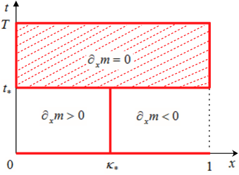
Figure 2. Profile of $\partial_{x}m$ defined by (1.12), where the red shaded area and red solid lines together represent the set $\{(x,t)\in[0,1]\times[0,T]:\partial_{x}m(x,t)=0\}$.

1.4. Discussion

The spatially and temporally degenerate advection are separately considered in Theorems 1.2 and 1.3. In fact, our ideas in the paper can deal with the case when the advection $m$ possesses both spatial and temporal degeneracy. Below we provide an example as an illustration. Assume $m$ takes the form of (1.9), and there are constants $0<\kappa_{1}<\kappa_{2}<1$ and $0<t_{*}<T$ such that

$$m_{2}(t)>0\ \text{ in }\,\left(0,t_{*}\right)\,\text{ and }\,m_{2}(t)\equiv 0\ \text{ in }\,\left[t_{*},T\right],\ \ \text{(Temporal degeneracy)},$$

$$m_{1}^{\prime}(x)>0\,\text{ in }\,\left[0,\kappa_{1}\right),\quad m_{1}^{\prime}(x)\equiv 0\text{ in }\,[\kappa_{1},\kappa_{2}]\,\,\text{ and }\,\,m_{1}^{\prime}(x)<0\,\text{ in }\,\left(\kappa_{2},1\right],\ \ \text{(Spatial degeneracy)}.$$

See Fig. 3 for the profile of the spatio-temporally degenerate $\partial_{x}m$. Combining the proofs of Propositions 4.1 and 5.1, one can prove that $\lambda(\alpha)\to\tilde{\lambda}_{*}$ as $\alpha\to\infty$, where $\tilde{\lambda}_{*}$ denotes the principal eigenvalue of the problem

(1.13) $$\left\{\begin{array}[]{ll}\vskip 3.0pt plus 1.0pt minus 1.0pt\partial_{t}\psi-\partial_{xx}\psi+V\psi=\lambda\psi&{\mathrm{in}}\,\,[\kappa_{1},\kappa_{2}]\times\left(0,t_{*}\right],\\ \vskip 3.0pt plus 1.0pt minus 1.0pt\partial_{x}\psi(\kappa_{1},t)=\partial_{x}\psi(\kappa_{2},t)=0&{\mathrm{on}}\,\,\left(0,t_{*}\right],\\ \vskip 3.0pt plus 1.0pt minus 1.0pt\psi(x,t_{*}^{+})=\hat{\psi}(x,t_{*})&{\mathrm{on}}\,\,(0,1),\\ \vskip 3.0pt plus 1.0pt minus 1.0pt\partial_{t}\psi-\partial_{xx}\psi+V\psi=\lambda\psi&{\mathrm{in}}\,\,(0,1)\times\left(t_{*},T\right],\\ \vskip 3.0pt plus 1.0pt minus 1.0pt\partial_{x}\psi(0,t)=\partial_{x}\psi(1,t)=0&{\mathrm{on}}\,\,\left(t_{*},T\right],\\ \psi(x,0)=\psi(x,T)&{\mathrm{on}}\,\,(0,1),\end{array}\right.$$

where $\hat{\psi}(x,t_{*})$ is the extension of $\psi(x,t_{*})$ by setting $\hat{\psi}(x,t_{*})=\psi(\kappa_{1},t_{*})$ for $x\in[0,\kappa_{1})$ and $\hat{\psi}(x,t_{*})=\psi(\kappa_{2},t_{*})$ for $x\in(\kappa_{2},1]$. The existence and uniqueness of $\tilde{\lambda}_{*}$ follows from the same arguments as in Proposition A.1.

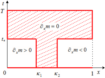
Figure 3. Profile of $\partial_{x}m$ for the spatio-temporally degenerate advection, where the red shaded area and red solid lines together represent the set $\{(x,t)\in[0,1]\times[0,T]:\partial_{x}m(x,t)=0\}$.

For general advection $m$, the cases of spatio-temporal degeneracies are so many that we can not address them specifically or state the results in a general theorem. This is merely a technical point which does not involve many new ideas, and thus is left to the interested reader. Moreover, the techniques developed in this paper can be used to investigate the asymptotic behaviors of the principal eigenvalue for (1.1) subject to other boundary conditions, including the zero Dirichlet boundary conditions and the Robin boundary conditions.

Our proofs in this paper rely heavily upon the construction of (almost) optimal pairs of sub-solutions and super-solutions in the sense of Definition 2.1, and applications of Proposition 2.1. To clarify the ideas, instead of proving Theorems 1.1-1.3 directly, we shall provide the detailed proof for some typical examples and the three main theorems follow by a similar argument.

1.5. Organization of the paper

In Sect. 2, we present the theory of weak sub-solutions and super-solutions. In Sect. 3, we discuss the nondegenerate advection and prove Theorem 1.1. Sect. 4 concerns spatially degenerate advection and Theorem 1.2 is proved there. The temporally degenerate advection is considered in Sect. 5 and Theorem 1.3 is proved, which requires more delicate analysis. Finally, we verify the existence and uniqueness of the principal eigenvalue for problem (1.11) in Appendix A, and prove (4.8) in Appendix B.

2. Generalized super/sub-solution for a time-periodic parabolic operator

In this section, we introduce the definition of super/sub-solution for a time-periodic parabolic operator, and then establish the relation of positive super/sub-solution and the sign of principal eigenvalue of an associated eigenvalue problem. This result is a generalization of Proposition 2.1 and Corollary 2.1 in [43] in one-dimensional case, and plays a vital role in the establishment of main findings in the present paper.

Let $\mathcal{L}$ denote the following linear parabolic operator on $(0,1)\times\mathbb{R}$:

(2.1) $$\mathcal{L}=\partial_{t}\varphi-a_{1}(x,t)\partial_{xx}-a_{2}(x,t)\partial_{x}+a_{0}(x,t).$$

We always assume $a_{1}(x,t)>0$ so that $\mathcal{L}$ is uniformly elliptic for each $t\in\mathbb{R}$, and assume $a_{0},a_{1},a_{2}\in C([0,1]\times\mathbb{R})$ are $T$-periodic with respect to $t$.

Consider the linear parabolic problem

(2.2) $$\left\{\begin{array}[]{ll}\vskip 3.0pt plus 1.0pt minus 1.0pt\mathcal{L}\varphi=0&{\text{in}}\,\,(0,1)\times[0,T],\\ \vskip 3.0pt plus 1.0pt minus 1.0pt\partial_{x}\varphi(0,t)=\partial_{x}\varphi(1,t)=0&{\text{on}}\,\,[0,T],\\ \varphi(x,0)=\varphi(x,T)&{\text{on}}\,\,(0,1).\end{array}\right.$$

We now give the definition of super/sub-solution corresponding to (2.2).

Definition 2.1.

The lower semi-continuous function $\overline{\varphi}$ in $[0,1]\times[0,T]$ is called a super-solution of (2.2) if there exist sets $\mathbb{X}$ and $\mathbb{T}$ consisting of at most finitely many continuous curves:

$$\mathbb{X}=\emptyset\text{ or }\mathbb{X}=\left\{(\kappa_{i}(t),t):\ \,t\in(0,T),\ i=1,\ldots,N\right\},$$

$$\mathbb{T}=\emptyset\text{ or }\mathbb{T}=\left\{(x,\tau_{i}(x)):\ \,x\in(0,1),\ i=1,\ldots,M\right\},$$

for some integers $N,M\geq 1$, where the continuous functions $\kappa_{i}:\ [0,T]\mapsto(0,1)$ and $\tau_{i}:\ [0,1]\mapsto(0,T)$ are such that

(1) $\overline{\varphi}\in C\left((0,1)\times(0,T)\setminus\mathbb{T}\right)\cap C^{2}\left((0,1)\times(0,T)\setminus\left(\mathbb{X}\cup\mathbb{T}\right)\right)$;

(2) $\partial_{x}\overline{\varphi}(x^{+},t)<\partial_{x}\overline{\varphi}(x^{-},t)$, $\forall(x,t)\in\mathbb{X};$

(3) $\overline{\varphi}(x,t)=\overline{\varphi}(x,t^{-})<\overline{\varphi}(x,t^{+})$ or $\overline{\varphi}(x,t^{-})=\overline{\varphi}(x,t^{+})$ but $\partial_{t}\overline{\varphi}(x,t^{+})<\partial_{t}\overline{\varphi}(x,t^{-})$, $\forall(x,t)\in\mathbb{T};$

(4) $\overline{\varphi}$ satisfies

(2.3) $$\left\{\begin{array}[]{ll}\vskip 3.0pt plus 1.0pt minus 1.0pt\mathcal{L}\overline{\varphi}\geq 0&{\mathrm{in}}\,\,((0,1)\times(0,T))\setminus\left(\mathbb{X}\cup\mathbb{T}\right),\\ \vskip 3.0pt plus 1.0pt minus 1.0pt\partial_{x}\overline{\varphi}(0,t)\leq 0,\ \ \partial_{x}\overline{\varphi}(1,t)\geq 0&{\mathrm{on}}\,\,[0,T],\\ \overline{\varphi}(x,0)\geq\overline{\varphi}(x,T)&\mathrm{on}\,\,(0,1).\end{array}\right.$$

A super-solution $\overline{\varphi}$ is called a strict super-solution if it is not a solution of (2.2). Moreover, a function $\underline{\varphi}$ is called a (strict) sub-solution of (2.2) if $-\underline{\varphi}$ is a (strict) super-solution.

Lemma 2.1.

Let $\overline{\varphi}\geq 0$ be a super-solution of (2.2) defined in Definition 2.1. Then $\overline{\varphi}>0$ in $[0,1]\times[0,T]$ unless $\overline{\varphi}\equiv 0$.

Proof.

Assume that $\overline{\varphi}\not\equiv 0$ and we shall prove $\overline{\varphi}>0$ in $[0,1]\times[0,T]$. First, by the Hopf’s boundary lemma for parabolic equations (see e.g. [18, Proposition 13.3]), we deduce $\overline{\varphi}>0$ on the boundary $\{0,1\}\times[0,T]$.

Suppose the assertion fails, then there exists some interior point $(x_{0},t_{0})\in(0,1)\times[0,T]$ such that (i) $\overline{\varphi}(x_{0},t_{0})=0$ and (ii) $x_{0}\in\partial\{x\in\Omega:\overline{\varphi}(x,t_{0})=0\}$. This is possible since $\overline{\varphi}>0$ on the boundary $\{0,1\}\times[0,T]$. We mention that such point $(x_{0},t_{0})$ can be chosen such that $t_{0}>0$. Indeed, if $t_{0}=0$, the fact that $\overline{\varphi}(x_{0},0)\geq\overline{\varphi}(x_{0},T)$ implies $\overline{\varphi}(x_{0},T)=0$. Then we can select some $(\tilde{x}_{0},T)$, satisfying (i) and (ii), to replace $(x_{0},t_{0})$.

Next, we claim that $(x_{0},t_{0})\not\in\mathbb{X}\cup\mathbb{T}$. If $(x_{0},t_{0})\in\mathbb{X}$, by (2) in Definition 2.1, it holds that $\partial_{x}\overline{\varphi}(x_{0}^{+},t_{0})<\partial_{x}\overline{\varphi}(x_{0}^{-},t_{0})\leq 0$. Since $\overline{\varphi}(x_{0},t_{0})=0$, this contradicts $\overline{\varphi}\geq 0$. If $(x_{0},t_{0})\in\mathbb{T}$, in light of (3) in Definition 2.1, we distinguish two cases: (a) $\overline{\varphi}(x_{0},t_{0}^{-})<\overline{\varphi}(x_{0},t_{0}^{+})$ and (b) $\overline{\varphi}(x_{0},t_{0}^{-})=\overline{\varphi}(x_{0},t_{0}^{+})$ to reach a contradiction. When (a) occurs, by (3), $\overline{\varphi}(x_{0},t_{0}^{-})=\overline{\varphi}(x_{0},t_{0})=0$. Choose $\delta_{1}\in(0,\delta)$ small such that $B_{\delta_{1}}^{+}:=B_{\delta_{1}}(x_{0},t_{0})\cap((0,1)\times[0,t_{0}))$ satisfies $B_{\delta_{1}}^{+}\cap(\mathbb{X}\cup\mathbb{T})=\emptyset$,

$$\mathcal{L}\overline{\varphi}\geq 0\,\,\text{ in }\,\,B_{\delta_{1}}^{+}\quad\text{and}\quad\overline{\varphi}(x_{0},t_{0}^{-})=0.$$

We may apply the classical strong maximum principle for parabolic equations (see e.g. Proposition 13.1 and Remark 13.2 in [18]) to arrive at $\overline{\varphi}\equiv 0$ in $\overline{B}_{\delta_{1}}^{+}$. This contradicts to (ii). When (b) occurs, by our assumption, $\partial_{t}\overline{\varphi}(x_{0},t_{0}^{+})<\partial_{t}\overline{\varphi}(x_{0},t_{0}^{-})\leq 0$, which together with (i) contradicts $\overline{\varphi}\geq 0$. Hence, $(x_{0},t_{0})\not\in\mathbb{X}\cup\mathbb{T}$.

Therefore, there exists some $\delta_{2}\in(0,\delta)$ such that $B_{\delta_{2}}(x_{0},t_{0})\cap\left(\mathbb{X}\cup\mathbb{T}\right)=\emptyset$ and

$$\mathcal{L}\overline{\varphi}\geq 0\,\,\text{ in}\,\,B_{\delta_{2}}(x_{0},t_{0})\,\,\text{ and }\,\,\overline{\varphi}(x_{0},t_{0})=0.$$

Due to $t_{0}>0$, by the classical strong maximum principal, we can conclude that $\overline{\varphi}\equiv 0$ in $B_{\delta_{2}}(x_{0},t_{0})\cap([0,1]\times[0,t_{0}])$, a contradiction to (ii) again. The proof is now complete. ∎

Consider the following eigenvalue problem:

(2.4) $$\left\{\begin{array}[]{ll}\vskip 6.0pt plus 2.0pt minus 2.0pt\mathcal{L}\varphi=\lambda(\mathcal{L})\varphi&{\text{in}}\,\,(0,1)\times[0,T],\\ \vskip 6.0pt plus 2.0pt minus 2.0pt\partial_{x}\varphi(0,t)=\partial_{x}\varphi(1,t)=0&{\text{on}}\,\,[0,T],\\ \varphi(x,0)=\varphi(x,T)&\text{on}\,\,(0,1).\end{array}\right.$$

The main result in this section can be stated as follows.

Proposition 2.1.

Let $\lambda(\mathcal{L})$ denote the principal eigenvalue of (2.4). If (2.2) admits some strict positive super-solution defined in Definition 2.1, then $\lambda(\mathcal{L})\geq 0$. Moreover, if (2.2) admits some strict nonnegative sub-solution defined in Definition 2.1, then $\lambda(\mathcal{L})\leq 0$.

Thanks to Lemma 2.1, Proposition 2.1 can be proved by the same arguments as in Proposition 2.1 and Corollary 2.1 of [43], where the equivalent relationship of $\lambda(\mathcal{L})>0$ and a positive strict (classical) super-solution, is established. Such an idea can be traced back to Walter [50] for the elliptic operators under zero Dirichlet boundary conditions. We omit the details and refer interested readers to [43].

3. Nondegenerate advection: proof of Theorem 1.1

This section is devoted to the proof of Theorem 1.1 which concerns the case that all critical points of advection function $m$ are nondegenerate. The results for a typical example will be proved first, and then Theorem 1.1 follows from a similar argument. From now on, we shall use $\mathcal{L}_{\alpha}$ to denote the following time-periodic parabolic operator:

$$\mathcal{L}_{\alpha}:=\partial_{t}-\partial_{xx}-\alpha\partial_{x}m\cdot\partial_{x}+V,\ \ (\alpha\geq 0).$$

Our first result concerns the following special case:

Proposition 3.1.

Suppose that there exist $T$-periodic functions $\kappa_{i}\in C^{1}(\mathbb{R})$ ($i=1,2,3$) such that $0\leq\kappa_{1}(t)<\kappa_{2}(t)<\kappa_{3}(t)\leq 1$ for all $t\in[0,T]$ and

(3.1) $$\begin{cases}\partial_{x}m(x,t)>0,\ \ &x\in\left(0,\kappa_{1}(t)\right)\cup\left(\kappa_{2}(t),\kappa_{3}(t)\right),\,\,\,t\in[0,T],\\ \partial_{x}m(x,t)=0,\ \ &x=\kappa_{1}(t),\,\kappa_{2}(t),\,\kappa_{3}(t),\,\,\,t\in[0,T],\\ \partial_{x}m(x,t)<0,\ \ &x\in\left(\kappa_{1}(t),\kappa_{2}(t)\right)\cup\left(\kappa_{3}(t),1\right),\,\,\,t\in[0,T].\end{cases}$$

Let $\lambda(\alpha)$ be the principal eigenvalue of (1.1). Then

$$\lim_{\alpha\rightarrow\infty}\lambda(\alpha)=\min\left\{\frac{1}{T}\int_{0}^{T}V\left(\kappa_{1}(s),s\right)\mathrm{d}s,\ \ \frac{1}{T}\int_{0}^{T}V\left(\kappa_{3}(s),s\right)\mathrm{d}s\right\}.$$

Proof.

Without loss of generality, assume that

(3.2) $$\int_{0}^{T}V\left(\kappa_{1}(s),s\right)\mathrm{d}s\leq\int_{0}^{T}V\left(\kappa_{3}(s),s\right)\mathrm{d}s.$$

It suffices to show $\lambda(\alpha)\to\frac{1}{T}\int_{0}^{T}V\left(\kappa_{1}(s),s\right)\mathrm{d}s$ as $\alpha\rightarrow\infty$. We divide the proof into two steps.

Step 1. We first prove

(3.3) $$\liminf_{\alpha\to\infty}\lambda(\alpha)\geq\frac{1}{T}\int_{0}^{T}V\left(\kappa_{1}(s),s\right)\mathrm{d}s.$$

We shall construct a positive super-solution $\overline{\varphi}$ in the sense of Definition 2.1. More precisely, for any given small constant $\epsilon>0$, we devote ourselves to identifying the curve set $\mathbb{X}$ there and constructing a continuous function $\overline{\varphi}>0$ such that

(3.4) $$\left\{\begin{array}[]{ll}\vskip 6.0pt plus 2.0pt minus 2.0pt\mathcal{L}_{\alpha}\overline{\varphi}\geq\left[{1\over T}\int_{0}^{T}V\left(\kappa_{1}(s),s\right)\mathrm{d}s-\epsilon\right]\overline{\varphi}&\text{in}\,\,\left((0,1)\times[0,T]\right)\setminus\mathbb{X},\\ \vskip 6.0pt plus 2.0pt minus 2.0pt\partial_{x}\overline{\varphi}(0,t)\leq 0,\ \ \partial_{x}\overline{\varphi}(1,t)\geq 0&\text{on}\,\,[0,T],\\ \vskip 6.0pt plus 2.0pt minus 2.0pt\overline{\varphi}(x,0)=\overline{\varphi}(x,T)&\text{on}\,\,(0,1),\\ \partial_{x}\overline{\varphi}(x^{+},t)<\partial_{x}\overline{\varphi}(x^{-},t)&\text{in}\,\,\mathbb{X},\end{array}\right.$$

provided that $\alpha>0$ is sufficiently large. Once such a super-solution $\overline{\varphi}$ exists, a direct application of Proposition 2.1 to the operator $\mathcal{L}:=\mathcal{L}_{\alpha}-\left[{1\over T}\int_{0}^{T}V\left(\kappa_{1}(s),s\right)\mathrm{d}s-\epsilon\right]$ yields (3.3).

To this end, we introduce some constant $\delta$ with $0<\delta\ll 1$ such that

(3.5) $$|V(x,t)-V\left(\kappa_{i}(t),t\right)|<\epsilon/2\ \ \text{ on }\Delta_{i\delta}:=\{(x,t)\in[0,1]\times[0,T]:|x-\kappa_{i}(t)|<\delta\},\,\,i=1,2,3.$$

We construct $\overline{\varphi}$ on different regions of $[0,1]\times[0,T]$.

$\mathbf{(1)}$ For $(x,t)\in\Delta_{1\delta}$, we define

(3.6) $$\overline{\varphi}(x,t):=\overline{z}_{1}(x,t)f_{1}(t),$$

where $f_{1}$ is a $T$-periodic function given by

(3.7) $$\begin{array}[]{ll}\displaystyle f_{1}(t)=\exp\left[{-\int_{0}^{t}V\left(\kappa_{1}(s),s\right)\mathrm{d}s+{t\over T}\int_{0}^{T}V\left(\kappa_{1}(s),s\right)\mathrm{d}s}\right].\end{array}$$

To verify the first inequality in (3.4), by (3.6) we need to find $\overline{z}_{1}>0$ such that

(3.8) $$\begin{array}[]{ll}\partial_{t}\overline{z}_{1}-\partial_{xx}\overline{z}_{1}-\alpha\partial_{x}m\partial_{x}\overline{z}_{1}+\left[V-V\left(\kappa_{1},t\right)+\epsilon\right]\overline{z}_{1}>0\quad\text{ on }\,\Delta_{1\delta}.\end{array}$$

Indeed, set

$$\overline{z}_{1}(x,t):=M_{1}+\left(x-\kappa_{1}(t)\right)^{2},$$

where $M_{1}$ is chosen such that $\epsilon M_{1}>4+4\delta\|\kappa_{1}^{\prime}\|_{\infty}$. By our assumption (3.1), it is noted that

$$-\alpha\partial_{x}m\cdot\partial_{x}\overline{z}_{1}=-2\alpha\left(x-\kappa_{1}(t)\right)\partial_{x}m\geq 0\quad\text{ on }\,\Delta_{1\delta},$$

and by (3.5), $V(x,t)-V\left(\kappa_{1},t\right)+\epsilon\geq\epsilon/2$. Hence, by the choice of $M_{1}$ we can verify (3.8), so that the chosen $\overline{\varphi}$ in (3.6) satisfies (3.4) on $\Delta_{1\delta}$ for all $\alpha>0$.

$\mathbf{(2)}$ For $(x,t)\in\Delta_{3\delta}$ as above, we construct

$$\overline{\varphi}(x,t):=\overline{z}_{3}(x,t)f_{3}(t),$$

with $T$-periodic function $f_{3}$ given by

$$\begin{array}[]{ll}\displaystyle f_{3}(t)=\exp\left[{-\int_{0}^{t}V\left(\kappa_{3}(s),s\right)\mathrm{d}s+{t\over T}\int_{0}^{T}V\left(\kappa_{3}(s),s\right)\mathrm{d}s}\right].\end{array}$$

Set $\overline{z}_{3}(x,t):=M_{3}+\left(x-\kappa_{3}(t)\right)^{2}$. It can be checked that for large $M_{3}$ (independent of $\alpha>0$),

$$\begin{array}[]{ll}\partial_{t}\overline{z}_{3}-\partial_{xx}\overline{z}_{3}-\alpha\partial_{x}m\partial_{x}\overline{z}_{3}+\left[V-V\left(\kappa_{3},t\right)+\epsilon\right]\overline{z}_{3}>0\quad\text{ on }\,\Delta_{3\delta},\end{array}$$

which together with (3.2) implies that the constructed $\overline{\varphi}$ satisfies (3.8) on $\Delta_{3\delta}$ for any $\alpha>0$.

$\mathbf{(3)}$ For $(x,t)\in\Delta_{2\delta}$, we construct $\overline{\varphi}$ in the form of

$$\overline{\varphi}(x,t):=M_{2}\left[1-\frac{\left(x-\kappa_{2}(t)\right)^{2}}{2\delta^{2}}\right],$$

where we may choose $\delta>0$ further small if necessarily such that

(3.9) $$\delta\|\kappa^{\prime}_{2}\|_{\infty}+\delta^{2}\left\|V-{1\over T}\int_{0}^{T}V\left(\kappa_{1}(s),s\right)\mathrm{d}s+\epsilon\right\|_{\infty}<1.$$

and the constant $M_{2}$ is chosen to satisfy

$$M_{2}>2\max\Big{\{}\|\overline{\varphi}\left(\kappa_{1}(\cdot)+\delta,\cdot\right)\|_{\infty},\ \|\overline{\varphi}\left(\kappa_{3}(\cdot)-\delta,\cdot\right)\|_{\infty}\Big{\}}$$

with $\overline{\varphi}\left(\kappa_{1}+\delta,\cdot\right)$ and $\overline{\varphi}\left(\kappa_{3}-\delta,\cdot\right)$ being defined in $\mathbf{(1)}$ and $\mathbf{(2)}$. Thus for each $t\in[0,T]$, we have

(3.10) $$\begin{array}[]{l}\overline{\varphi}(\kappa_{2}(t)-\delta,t)>\overline{\varphi}\left(\kappa_{1}(t)+\delta,t\right)\quad\text{and }\quad\overline{\varphi}(\kappa_{2}(t)+\delta,t)>\overline{\varphi}(\kappa_{3}(t)-\delta,t).\end{array}$$

In view of $-\partial_{x}m\partial_{x}\overline{\varphi}\geq 0$ on $\Delta_{2\delta}$, direct calculation yields that for any $\alpha>0$,

$$\begin{array}[]{l}\vskip 3.0pt plus 1.0pt minus 1.0pt\quad\displaystyle\mathcal{L}_{\alpha}\overline{\varphi}-\left[\frac{1}{T}\int_{0}^{T}V\left(\kappa_{1}(s),s\right)\mathrm{d}s-\epsilon\right]\overline{\varphi}\\ \vskip 3.0pt plus 1.0pt minus 1.0pt=\displaystyle\frac{M_{2}}{\delta^{2}}(x-\kappa_{2})\kappa^{\prime}_{2}+\frac{M_{2}}{\delta^{2}}-\alpha\partial_{x}m\partial_{x}\overline{\varphi}+\left[V-{1\over T}\int_{0}^{T}V\left(\kappa_{1}(s),s\right)\mathrm{d}s+\epsilon\right]\overline{\varphi}\\ \vskip 3.0pt plus 1.0pt minus 1.0pt\geq\displaystyle\frac{M_{2}}{\delta^{2}}-\frac{M_{2}}{\delta}\|\kappa^{\prime}_{2}\|_{\infty}-M_{2}\left\|V-{1\over T}\int_{0}^{T}V\left(\kappa_{1}(s),s\right)\mathrm{d}s+\epsilon\right\|_{\infty}\\ >0\qquad\text{on }\,\Delta_{2\delta},\end{array}$$

where the last inequality is due to the choice of $\delta$ in (3.9).

$\mathbf{(4)}$ For $(x,t)\in((0,1)\times[0,T])\setminus(\Delta_{1\delta}\cup\Delta_{2\delta}\cup\Delta_{3\delta})$, there is a constant $\rho>0$ independent of $(x,t)$ such that $|\partial_{x}m|>\rho$ and we shall construct the super-solution $\overline{\varphi}$ on this region by monotonically connecting the endpoints on $\partial\Delta_{i\delta}$ ($i=1,2,3$). Taking $\left\{(x,t):x\in[\kappa_{1}(t)+\delta,\kappa_{2}(t)-\delta\right],\,t\in[0,T]\}$ as an example, by (3.10), we may construct $\overline{\varphi}$ to be a positive $T$-periodic continuous function such that $\partial_{x}\overline{\varphi}>0$ in this region and

(3.11) $$\partial_{x}\overline{\varphi}((\partial\Delta_{i\delta})^{+},t)<\partial_{x}\overline{\varphi}((\partial\Delta_{i\delta})^{-},t),\quad i=1,2.$$

Due to $-\alpha\partial_{x}m\partial_{x}\overline{\varphi}>\alpha\rho\partial_{x}\overline{\varphi}$, we can verify that such a function $\overline{\varphi}$ verifies $\mathcal{L}\overline{\varphi}>0$ by choosing $\alpha>0$ large. Similar constructions can be applied to the other remaining regions.

Now we have constructed the desired strict super-solution $\overline{\varphi}$ satisfying (3.4) with $\mathbb{X}=\partial\Delta_{1\delta}\cup\partial\Delta_{2\delta}\cup\partial\Delta_{3\delta}$ The profile of $\overline{\varphi}$ defined in $\mathbf{(1)}$-$\mathbf{(4)}$ can be illustrated in Fig. 4. Therefore, the assertion (3.3) is a direct consequence of Proposition 2.1.

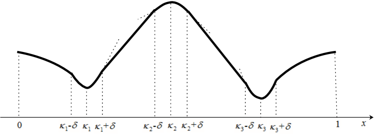
Figure 4. Profile of the constructed $\overline{\varphi}$ for fixed $t$.

Step 2. We next prove

(3.12) $$\limsup_{\alpha\to\infty}\lambda(\alpha)\leq\frac{1}{T}\int_{0}^{T}V\left(\kappa_{1}(s),s\right)\mathrm{d}s.$$

We employ a similar strategy as in Step 1. Given any small $\epsilon>0$, we shall construct a strict sub-solution $\underline{\varphi}\geq 0$ that satisfies for large $\alpha>0$,

(3.13) $$\left\{\begin{array}[]{ll}\vskip 6.0pt plus 2.0pt minus 2.0pt\mathcal{L}_{\alpha}\underline{\varphi}\leq\left[{1\over T}\int_{0}^{T}V\left(\kappa_{1}(s),s\right)\mathrm{d}s+\epsilon\right]\underline{\varphi}&\text{in}\,\,\left((0,1)\times[0,T]\right)\setminus\mathbb{X},\\ \vskip 6.0pt plus 2.0pt minus 2.0pt\partial_{x}\underline{\varphi}(0,t)\geq 0,\ \ \partial_{x}\underline{\varphi}(1,t)\leq 0,&\text{on}\,\,[0,T],\\ \underline{\varphi}(x,0)=\underline{\varphi}(x,T)&\text{on}\,\,(0,1),\end{array}\right.$$

where $\mathbb{X}$ will be determined below so that $\partial_{x}\underline{\varphi}(x^{+},t)>\partial_{x}\underline{\varphi}(x^{-},t)$ for all $(x,t)\in\mathbb{X}$. Once such a sub-solution $\underline{\varphi}$ exists, by Proposition 2.1 one can obtain (3.12). For the sake of clarity, we assume $0<\kappa_{1}(t)<\kappa_{2}(t)<\kappa_{3}(t)<1$ for all $t\in[0,T]$, as it is easily seen that the following construction also work for other cases.

To this end, we proceed as in Step 1 to find $\underline{z}\geq 0$ such that

(3.14) $$\left\{\begin{array}[]{ll}\vskip 6.0pt plus 2.0pt minus 2.0pt\partial_{t}\underline{z}-\partial_{xx}\underline{z}-\alpha\partial_{x}m\partial_{x}\underline{z}+\left[V-V\left(\kappa_{1}(t),t\right)-\epsilon\right]\underline{z}\leq 0,\,\not\equiv 0&\text{ in }((0,1)\times[0,T])\setminus\mathbb{X},\\ \displaystyle\partial_{x}\underline{z}(0,t)\geq 0,\ \ \partial_{x}\underline{z}_{x}(1,t)\leq 0&\text{ on }[0,T],\end{array}\right.$$

so that $\underline{\varphi}(x,t):=\underline{z}(x,t)f_{1}(t)$ is a sub-solution satisfying (3.13), where $f_{1}$ is given by (3.7). For this purpose, we define $\underline{z}\in C([0,1]\times[0,T])$ by

$$\underline{z}(x,t):=\begin{cases}\vskip 3.0pt plus 1.0pt minus 1.0pt1+\frac{\epsilon\delta^{2}}{16}-\frac{\epsilon}{4}\left(x-\kappa_{1}(t)\right)^{2},&x\in\left[\kappa_{1}(t)-\frac{\delta}{2},\kappa_{1}(t)+\frac{\delta}{2}\right],t\in[0,T],\\ \vskip 3.0pt plus 1.0pt minus 1.0pt\underline{z}_{1}(x,t),&x\in\left(\kappa_{1}(t)-\delta,\kappa_{1}(t)-\frac{\delta}{2}\right),t\in[0,T],\\ \vskip 3.0pt plus 1.0pt minus 1.0pt\underline{z}_{2}(x,t),&x\in\left(\kappa_{1}(t)+\frac{\delta}{2},\kappa_{1}(t)+\delta\right),t\in[0,T],\\ 0,&x\notin\left(\kappa_{1}(t)-\delta,\kappa_{1}(t)+\delta\right),\end{cases}$$

where $\delta>0$ is defined in Step 1 such that (3.5) holds. For any $x\in\left[\kappa_{1}(t)-\frac{\delta}{2},\kappa_{1}(t)+\frac{\delta}{2}\right]$ and $t\in[0,T]$, noting from (3.1) that $\partial_{x}m\partial_{x}\underline{z}\geq 0$, by choosing $\delta$ further small if necessarily we can verify (3.14) holds. For any $t\in[0,T]$, we then choose $\underline{z}_{1}$ and $\underline{z}_{2}$ to fulfill the following properties:

$$\begin{cases}\vskip 3.0pt plus 1.0pt minus 1.0pt\partial_{x}\underline{z}_{1}(x,t)>0,\ \ \ \ \ \ x\in\left(\kappa_{1}(t)-\delta,\kappa_{1}(t)-\frac{\delta}{2}\right),\\ \vskip 3.0pt plus 1.0pt minus 1.0pt\underline{z}_{1}\left(\kappa_{1}(t)-\delta,t\right)=0,\ \ \ \underline{z}_{1}\left(\kappa_{1}(t)-\frac{\delta}{2},t\right)=1,\\ \vskip 3.0pt plus 1.0pt minus 1.0pt\partial_{x}\underline{z}_{1}\left(\left(\kappa_{1}-\delta/2,t\right)^{-}\right)<\frac{\epsilon\delta}{4}=\partial_{x}\underline{z}_{1}\left(\left(\kappa_{1}-\delta/2,t\right)^{+}\right),\end{cases}$$

and

$$\begin{cases}\vskip 3.0pt plus 1.0pt minus 1.0pt\partial_{x}\underline{z}_{2}(x,t)<0,\ \ \ \ \ \ x\in\left(\kappa_{1}(t)+\frac{\delta}{2},\kappa_{1}(t)+\delta\right),\\ \vskip 3.0pt plus 1.0pt minus 1.0pt\underline{z}_{2}\left(\kappa_{1}(t)+\delta,t\right)=0,\ \ \ \underline{z}_{2}\left(\kappa_{1}(t)+\frac{\delta}{2},t\right)=1,\\ \vskip 3.0pt plus 1.0pt minus 1.0pt\partial_{x}\underline{z}_{1}\left(\left(\kappa_{1}+\delta/2\right)^{+},t\right)>-\frac{\epsilon\delta}{4}=\partial_{x}\underline{z}_{1}\left(\left(\kappa_{1}+\delta/2\right)^{-},t\right).\end{cases}$$

Note that $|\partial_{x}m|>\rho>0$ for some $\rho>0$ independent of $(x,t)$. Similar to $\mathbf{(4)}$ in Step 1, it can be verified readily that $\underline{z}$ satisfies (3.14) with

$$\begin{array}[]{l}\mathbb{X}=\Big{\{}(\kappa_{1}(t)\pm\delta,t),\ (\kappa_{1}(t)\pm\frac{\delta}{2},t):\,t\in[0,T]\Big{\}}.\end{array}$$

Thus our analysis above implies (3.12).

As a consequence, Proposition 3.1 follows from (3.3) and (3.12). ∎

Remark 3.1.

(1) Let $\kappa_{1}\equiv 0$ and $\kappa_{3}\equiv 1$ in (3.1), i.e. $m$ satisfies

$$\begin{cases}\partial_{x}m(x,t)<0,\ \ &x\in\left(0,\kappa_{2}(t)\right),\,t\in[0,T],\\ \partial_{x}m(\kappa_{2}(t),t)=0,\ \ &t\in[0,T],\\ \partial_{x}m(x,t)>0,\ \ &x\in\left(\kappa_{2}(t),1\right),\,t\in[0,T]\end{cases}$$

with $\kappa_{2}\in C^{1}([0,T])$ satisfying $0<\kappa_{2}(t)<1$ for all $t\in[0,T]$. Then Proposition 3.1 yields $\lambda(\alpha)\to\min\left\{\frac{1}{T}\int_{0}^{T}V\left(0,s\right)\mathrm{d}s,\ \ \frac{1}{T}\int_{0}^{T}V\left(1,s\right)\mathrm{d}s\right\}$ as $\alpha\rightarrow\infty$.

(2) Let $\kappa_{2}$ and $\kappa_{3}$ in (3.1) tend to $1$, i.e. $m$ satisfies

(3.15) $$\begin{cases}\partial_{x}m(x,t)>0,\ \ &x\in\left(0,\kappa_{1}(t)\right),\,t\in[0,T],\\ \partial_{x}m(\kappa_{1}(t),t)=0,\ \ &t\in[0,T],\\ \partial_{x}m(x,t)<0,\ \ &x\in\left(\kappa_{1}(t),1\right),\,t\in[0,T]\end{cases}$$

with $\kappa_{1}\in C^{1}([0,T])$ satisfying $0\leq\kappa_{1}(t)\leq 1$ for $t\in[0,T]$. A illustrated example for such curve $\kappa_{1}$ can be shown in Fig. 5, where the case $\{t\in[0,T]:\kappa(t)=0\text{ or }\kappa(t)=1\}\neq\emptyset$ is allowed. By a similar but simpler argument as in Proposition 3.1, we can deduce $\lambda(\alpha)\to\frac{1}{T}\int_{0}^{T}V\left(\kappa_{1}(s),s\right)\mathrm{d}s$ as $\alpha\to\infty$. In particular, if $\kappa_{1}\equiv 0$ in (3.15), i.e. $\partial_{x}m<0$ in $\left(0,1\right)\times[0,T]$, we can conclude that $\lambda(\alpha)\to\frac{1}{T}\int_{0}^{T}V\left(0,s\right)\mathrm{d}s$ as $\alpha\to\infty$, which was first proved in [43, Theorem 1.1].

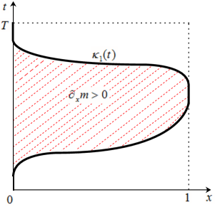
Figure 5. The profile of $\kappa_{1}$ in (3.15), as illustrated by the black solid curve. The red shaded region denotes the region where $\partial_{x}m>0$, while $\partial_{x}m<0$ in the white shaded region.

We are now in a position to prove Theorem 1.1.

Proof of Theorem 1.1.

Since all spatially critical points of $m$ are nondegenerate, by the implicit function theorem, it holds that $\kappa_{i}(t)\neq\kappa_{j}(t)$ for all $t\in[0,T]$ and $i\neq j$. Assume $0\leq\kappa_{1}(t)<\ldots<\kappa_{N}(t)\leq 1$. Then we can adopt directly the arguments developed in the proof of Propositions 3.1 to find a nonnegative sub-solution and a positive strict super-solution for problem (1.1). Finally, we may apply Proposition 2.1 to conclude Theorem 1.1. ∎

4. Spatially degenerate advection: Proof of Theorem 1.2

In this section, we are concerned with the case when the advection $m$ is spatially degenerate and prove Theorem 1.2. In particular, the set of local maximum points of $m$ allows some flat surfaces with respect to the spatial variable. The results in some typical cases will be presented and proved first, and Theorem 1.2 then follows by the similar arguments. Recall that $\lambda^{pq}\big{(}(\underline{\kappa},\overline{\kappa})\big{)}$ for $p,q\in\{\mathcal{N},\mathcal{D}\}$ denotes the principal eigenvalue of problem (1.6).

Proposition 4.1.

Suppose that there exist $T$-periodic functions $\kappa_{1},\kappa_{2}\in C^{1}(\mathbb{R})$ such that $0\leq\kappa_{1}(t)<\kappa_{2}(t)\leq 1$ for all $t\in[0,T]$ and

$$\begin{cases}\partial_{x}m(x,t)>0,\ \ &x\in\left(0,\kappa_{1}(t)\right),\,\,t\in[0,T],\\ \partial_{x}m(x,t)=0,\ \ &x\in[\kappa_{1}(t),\,\kappa_{2}(t)],\,\,t\in[0,T],\\ \partial_{x}m(x,t)<0,\ \ &x\in\left(\kappa_{2}(t),1\right),\,\,\,t\in[0,T].\end{cases}$$

Let $\lambda(\alpha)$ be the principal eigenvalue of (1.1). Then

$$\lim_{\alpha\rightarrow\infty}\lambda(\alpha)=\lambda^{\mathcal{N}\mathcal{N}}\big{(}(\kappa_{1},\kappa_{2})\big{)}.$$

The advection $m$ given in Proposition 4.1 can be illustrated in Fig. 6.

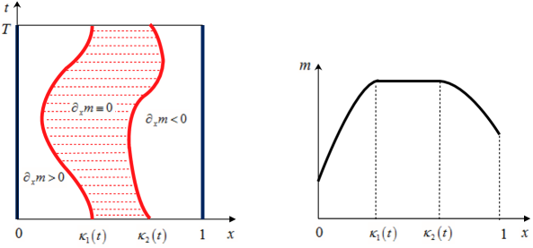
Figure 6. The profile of function $m$ given in Proposition 4.1. In the left side picture, the red colored curves correspond to functions $\kappa_{1},\kappa_{2}$ and the red shaded region denotes the region where $\partial_{x}m=0$. The black colored curve in the right side picture represents the graph of $m$ for fixed $t\in[0,T]$.

Proof of Proposition 4.1.

Given $\eta\in\mathbb{R}$, our analysis begins with the following auxiliary problem:

(4.1) $$\left\{\begin{array}[]{ll}\vskip 6.0pt plus 2.0pt minus 2.0pt\partial_{t}\psi-\partial_{xx}\psi+V(x,t)\psi=\lambda\psi,&x\in(\kappa_{1}(t),\,\kappa_{2}(t)),\,\,t\in[0,T],\\ \vskip 6.0pt plus 2.0pt minus 2.0pt\partial_{x}\psi\left(\kappa_{1},t\right)=\eta\psi\left(\kappa_{1},t\right),\partial_{x}\psi\left(\kappa_{2},t\right)=-\eta\psi\left(\kappa_{2},t\right),&t\in[0,T],\\ \psi(x,0)=\psi(x,T),&x\in\left[\kappa_{1}(0),\kappa_{2}(0)\right].\end{array}\right.$$

Denote by $\lambda^{\mathcal{N}}_{\eta}$ its principal eigenvalue and $\psi^{\mathcal{N}}_{\eta}>0$ the corresponding principal eigenfunction. It is well known that $\lambda^{\mathcal{N}}_{\eta}$ is increasing and analytical with respect to $\eta\in\mathbb{R}$. Clearly,

(4.2) $$\lim_{\eta\rightarrow 0}\lambda^{\mathcal{N}}_{\eta}=\lambda^{\mathcal{N}\mathcal{N}}\big{(}(\kappa_{1},\kappa_{2})\big{)},$$

and when $\eta<0$, it holds that $\partial_{x}\psi^{\mathcal{N}}_{\eta}\left(\kappa_{1}(t),t\right)<0$ and $\partial_{x}\psi^{\mathcal{N}}_{\eta}\left(\kappa_{2}(t),t\right)>0$ for all $t\in[0,T]$.

Step 1. We first prove

(4.3) $$\liminf_{\alpha\to\infty}\lambda(\alpha)\geq\lambda^{\mathcal{N}\mathcal{N}}\big{(}(\kappa_{1},\kappa_{2})\big{)}.$$

Inspired from the proof of Proposition 3.1, we shall construct a positive super-solution $\overline{\varphi}$, i.e. for any given constant $\eta<0$, we aim to find the curve set $\mathbb{X}$ and $\overline{\varphi}>0$ such that

(4.4) $$\left\{\begin{array}[]{ll}\vskip 6.0pt plus 2.0pt minus 2.0pt\mathcal{L}_{\alpha}\overline{\varphi}\geq\lambda^{\mathcal{N}}_{\eta}\overline{\varphi}&{\text{in}}\,\,\left((0,1)\times[0,T]\right)\setminus\mathbb{X},\\ \vskip 6.0pt plus 2.0pt minus 2.0pt\partial_{x}\overline{\varphi}(0,t)\leq 0,\ \ \partial_{x}\overline{\varphi}(1,t)\geq 0&{\text{on}}\,\,[0,T],\\ \vskip 6.0pt plus 2.0pt minus 2.0pt\overline{\varphi}(x,0)=\overline{\varphi}(x,T)&{\text{on}}\,\,(0,1),\\ \partial_{x}\overline{\varphi}(x^{+},t)<\partial_{x}\overline{\varphi}(x^{-},t)&\text{in}\,\,\mathbb{X}\end{array}\right.$$

for sufficiently large $\alpha>0$. Then (4.3) follows from Proposition 2.1. For this purpose, we first consider the case $0<\kappa_{1}<\kappa_{2}<1$ and construct $\overline{\varphi}$ on the following different regions.

$\mathbf{(1)}$ For $x\in\left[\kappa_{1}(t),\kappa_{2}(t)\right]$ and $t\in[0,T]$, we define $\overline{\varphi}(x,t):=\psi^{\mathcal{N}}_{\eta}(x,t)$ with $\eta<0$. In view of $\partial_{x}m(x,t)=0$, by the definition of $\psi^{\mathcal{N}}_{\eta}$ in (4.1), one can check that such a function $\overline{\varphi}$ satisfies $\mathcal{L}_{\alpha}\overline{\varphi}\geq\lambda^{\mathcal{N}}_{\eta}\overline{\varphi}$ on this region for all $\alpha>0$.

$\mathbf{(2)}$ For $x\in\left[\kappa_{1}(t)-\delta,\kappa_{1}(t)\right]$ and $t\in[0,T]$ with small $\delta>0$ to be determined later, we define

$$\begin{array}[]{l}\overline{\varphi}(x,t):=\psi^{\mathcal{N}}_{\eta}\left(\kappa_{1}(t),t\right)\left[1-\left(x-\kappa_{1}(t)\right)r-\left(x-\kappa_{1}(t)\right)^{2}R\right],\end{array}$$

where the constants $r,R>0$ will be specified below. Due to $\eta<0$, there holds $\partial_{x}\psi^{\mathcal{N}}_{\eta}\left(\kappa_{1}(t),t\right)<0$ for all $t\in[0,T]$. Fix $r>0$ small such that

$$\begin{array}[]{l}\partial_{x}\overline{\varphi}(\kappa_{1}^{-},t)=-r\psi^{\mathcal{N}}_{\eta}\left(\kappa_{1},t\right)>\partial_{x}\psi^{\mathcal{N}}_{\eta}\left(\kappa_{1},t\right)=\partial_{x}\overline{\varphi}(\kappa_{1}^{+},t),\ \,\forall t\in[0,T].\end{array}$$

Direct calculation gives

$$\begin{array}[]{ll}\vskip 6.0pt plus 2.0pt minus 2.0pt\mathcal{L}_{\alpha}\overline{\varphi}-\lambda^{\mathcal{N}}_{\eta}\overline{\varphi}=&\frac{{\rm d}\psi^{\mathcal{N}}_{\eta}\left(\kappa_{1},t\right)}{{\rm d}t}\left[1-\left(x-\kappa_{1}\right)r-\left(x-\kappa_{1}\right)^{2}R\right]+\psi^{\mathcal{N}}_{\eta}\left(\kappa_{1},t\right)\left[r\kappa^{\prime}_{1}+2R\left(x-\kappa_{1}\right)\kappa^{\prime}_{1}\right]\\ \vskip 6.0pt plus 2.0pt minus 2.0pt&-\alpha\partial_{x}m\cdot\psi^{\mathcal{N}}_{\eta}\left(\kappa_{1},t\right)\left[-r-2\left(x-\kappa_{1}\right)R\right]+2R\psi^{\mathcal{N}}_{\eta}\left(\kappa_{1},t\right)+V(x,t)\overline{\varphi}-\lambda^{\mathcal{N}}_{\eta}\overline{\varphi}.\end{array}$$

Set $R:=\frac{r}{2\delta}$. Since $\partial_{x}m(x,t)>0$ for $x\in\left[\kappa_{1}(t)-\delta,\kappa_{1}(t)\right)$, it holds that

$$\begin{array}[]{l}-\partial_{x}m\cdot\psi^{\mathcal{N}}_{\eta}\left(\kappa_{1},t\right)\left[-r-2\left(x-\kappa_{1}\right)R\right]\geq 0,\ \,\forall t\in[0,T],\end{array}$$

whence we calculate that

$$\begin{array}[]{ll}\vskip 6.0pt plus 2.0pt minus 2.0pt\displaystyle\mathcal{L}_{\alpha}\overline{\varphi}-\lambda^{\mathcal{N}}_{\eta}\overline{\varphi}\geq&\displaystyle-\left|\frac{{\rm d}\psi^{\mathcal{N}}_{\eta}\left(\kappa_{1},t\right)}{{\rm d}t}\right|\left(1+\frac{r\delta}{2}\right)-\frac{3r}{2}\psi^{\mathcal{N}}_{\eta}\left(\kappa_{1},t\right)|\kappa^{\prime}|+2R\psi^{\mathcal{N}}_{\eta}\left(\kappa_{1},t\right)\\ &\displaystyle-\left|V(x,t)-\lambda^{\mathcal{N}}_{\eta}\right|\psi^{\mathcal{N}}_{\eta}\left(\kappa_{1},t\right)\left(1+\frac{r\delta}{2}\right).\end{array}$$

We can choose $\delta$ small and thus $R$ large to obtain $\mathcal{L}_{\alpha}\overline{\varphi}\geq\lambda^{\mathcal{N}}_{\eta}\overline{\varphi}$ for all $\alpha>0$.

$\mathbf{(3)}$ For $x\in\left[0,\kappa_{1}(t)-\delta\right]$ and $t\in[0,T]$ with $\delta>0$ defined in $\mathbf{(2)}$, one may construct $\overline{\varphi}>0$ to be $T$-periodic and satisfy for each $t\in[0,T]$,

$$\begin{cases}\vskip 3.0pt plus 1.0pt minus 1.0pt\overline{\varphi}\left(\kappa_{1}(t)-\delta,t\right)=\psi^{\mathcal{N}}_{\eta}\left(\kappa_{1}(t),t\right)\left[1+r\delta-R\delta^{2}\right],\\ \vskip 3.0pt plus 1.0pt minus 1.0pt\partial_{x}\overline{\varphi}(x,t)<0,\quad x\in\left[0,\kappa_{1}(t)-\delta\right],\\ \partial_{x}\overline{\varphi}(\left(\kappa_{1}(t)-\delta\right)^{+},t)<\partial_{x}\overline{\varphi}(\left(\kappa_{1}(t)-\delta\right)^{-},t),\\ \end{cases}$$

where the first equality is to ensure the continuity of $\overline{\varphi}$. Noting that $|\partial_{x}m|>\rho$ for all $x\in\left[0,\kappa_{1}(t)-\delta\right]$ with some constant $\rho>0$ independent of $(x,t)$, we may deduce $\mathcal{L}_{\alpha}\overline{\varphi}\geq\lambda^{\mathcal{N}}_{\eta}\overline{\varphi}$ by choosing $\alpha>0$ large.

$\mathbf{(4)}$ For $x\in\left[\kappa_{2}(t),1\right]$ and $t\in[0,T]$, similar to $\mathbf{(2)}$ and $\mathbf{(3)}$, we can define $\overline{\varphi}$ as follow:

$$\begin{cases}\vskip 3.0pt plus 1.0pt minus 1.0pt\overline{\varphi}(x,t)=\psi^{\mathcal{N}}_{\eta}\left(\kappa_{2},t\right)\left[1+\tilde{r}\left(x-\kappa_{2}\right)+\tilde{R}\left(x-\kappa_{2}\right)^{2}\right],\,\,&x\in(\kappa_{2}(t),\kappa_{2}(t)+\delta),t\in[0,T],\\ \vskip 3.0pt plus 1.0pt minus 1.0pt\partial_{x}\overline{\varphi}(x,t)>0,\,\,&x\in\left[\kappa_{2}(t)+\delta,1\right],t\in[0,T],\\ \partial_{x}\overline{\varphi}(\left(\kappa_{2}+\delta\right)^{+},t)<\partial_{x}\overline{\varphi}(\left(\kappa_{2}+\delta\right)^{-},t),\ &t\in[0,T].\end{cases}$$

Proceeding as in $\mathbf{(2)}$ and $\mathbf{(3)}$, we can verify, by choosing small positive constants $\delta,\tilde{r}$ and large $\tilde{R}$, that $\mathcal{L}_{\alpha}\overline{\varphi}\geq\lambda^{\mathcal{N}}_{\eta}\overline{\varphi}$ for large $\alpha>0$.

By summarizing the above arguments, for the case $0<\kappa_{1}<\kappa_{2}<1$, we have constructed a strict super-solution $\overline{\varphi}>0$ satisfying (4.4) with

(4.5) $$\mathbb{X}=\Big{\{}(\kappa_{1}(t)-\delta,t),\,(\kappa_{1}(t),t),\,(\kappa_{2}(t),t),\,(\kappa_{2}(t)+\delta,t):\,t\in[0,T]\Big{\}}.$$

For the remaining case $\{t\in[0,T]:\kappa_{1}(t)=0\}\cup\{t\in[0,T]:\kappa_{2}(t)=1\}\neq\emptyset$, it can be verified that the above construction also work by noting that $\partial_{x}\psi^{\mathcal{N}}_{\eta}\left(\kappa_{1},t\right)<0$ and $\partial_{x}\psi^{\mathcal{N}}_{\eta}\left(\kappa_{2},t\right)>0$ for $\eta<0$. Therefore, applying Proposition 2.1, we conclude that for any $\eta<0$,

$$\liminf_{\alpha\to\infty}\lambda(\alpha)\geq\lambda^{\mathcal{N}}_{\eta},$$

which together with (4.2) gives the desired (4.3) by letting $\eta\searrow 0$. This completes Step 1.

Step 2. We prove

(4.6) $$\limsup_{\alpha\to\infty}\lambda(\alpha)\leq\lambda^{\mathcal{N}\mathcal{N}}\big{(}(\kappa_{1},\kappa_{2})\big{)}.$$

For each $\eta>0$, it suffices to find a strict sub-solution $\underline{\varphi}\geq 0$ such that for large $\alpha>0$,

(4.7) $$\left\{\begin{array}[]{ll}\vskip 6.0pt plus 2.0pt minus 2.0pt\mathcal{L}_{\alpha}\underline{\varphi}\leq\lambda^{\mathcal{N}}_{\eta}\underline{\varphi}&{\text{in}}\,\,\left((0,1)\times[0,T]\right)\setminus\mathbb{X},\\ \vskip 6.0pt plus 2.0pt minus 2.0pt\partial_{x}\underline{\varphi}(0,t)\geq 0,\ \ \partial_{x}\underline{\varphi}(1,t)\leq 0&{\text{on}}\,\,[0,T],\\ \vskip 6.0pt plus 2.0pt minus 2.0pt\underline{\varphi}(x,0)=\underline{\varphi}(x,T)&{\text{on}}\,\,(0,1),\end{array}\right.$$

and $\partial_{x}\underline{\varphi}(x^{+},t)>\partial_{x}\underline{\varphi}(x^{-},t)$ for all $(x,t)\in\mathbb{X}$, where $\mathbb{X}$ is defined by (4.5).

To this end, set $\underline{\varphi}(x,t):=\psi^{\mathcal{N}}_{\eta}(x,t)$ for $x\in\left[\kappa_{1}(t),\kappa_{2}(t)\right]$ and $t\in[0,T]$, where $\psi^{\mathcal{N}}_{\eta}>0$ denotes the principal eigenfunction of (4.1) with $\eta>0$. Since $\partial_{x}m(x,t)=0$, it follows that $\mathcal{L}_{\alpha}\underline{\varphi}\leq\lambda^{\mathcal{N}}_{\eta}\underline{\varphi}$ obviously. Observe that for any $\eta>0$,

$$\begin{array}[]{l}\partial_{x}\psi^{\mathcal{N}}_{\eta}\left(\kappa_{1},t\right)>0\quad\mathrm{and}\quad\partial_{x}\psi^{\mathcal{N}}_{\eta}\left(\kappa_{2},t\right)<0,\ \ \forall t\in[0,T].\end{array}$$

Such sub-solution $\underline{\varphi}$ satisfying (4.7) can be constructed by the similar arguments as in Step 1. Then we may apply Proposition 2.1 to deduce

$$\liminf_{\alpha\to\infty}\lambda(\alpha)\leq\lambda^{\mathcal{N}}_{\eta}\quad\text{for all }\eta>0.$$

for which sending $\eta\searrow 0$ implies (4.6) by using (4.2).

A combination of (4.3) and (4.6) yields Proposition 4.1, and the proof is complete. ∎

Remark 4.1.

When the strip $(\kappa_{1}(t),\kappa_{2}(t))$ in Proposition 4.1 shrinks to one curve $\kappa\in C^{1}(\mathbb{R})$ as illustrated in Fig. 7, we can assert that Proposition 4.1 coincides with the result in Remark 3.1(2) by the following observation:

(4.8) $$\lim_{\delta\rightarrow 0^{+}}\lambda^{\mathcal{N}\mathcal{N}}\big{(}(\kappa-\delta,\kappa+\delta)\big{)}=\frac{1}{T}\int_{0}^{T}V\left(\kappa(s),s\right)\mathrm{d}s.$$

The proof of (4.8) is given in Appendix B for the sake of completeness.

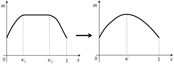
Figure 7. The profile of advection $m$ in Proposition 4.1 for fixed $t\in[0,T]$ as the two curve $\kappa_{1}$ and $\kappa_{2}$ shrink to $\kappa\in C(\mathbb{R})$.

Proposition 4.2.

Suppose that there exist $T$-periodic functions $\kappa_{1},\kappa_{2}\in C^{1}(\mathbb{R})$ such that $0\leq\kappa_{1}(t)<\kappa_{2}(t)\leq 1$ for all $t\in[0,T]$ and

$$\begin{cases}\partial_{x}m(x,t)<0,\ \ &x\in\left(0,\kappa_{1}(t)\right),\,t\in[0,T],\\ \partial_{x}m(x,t)=0,&x\in\left[\kappa_{1}(t),\kappa_{2}(t)\right],\,t\in[0,T],\\ \partial_{x}m(x,t)>0,&x\in\left(\kappa_{2}(t),1\right),\,t\in[0,T].\end{cases}$$

• If $0<\kappa_{1}(t)<\kappa_{2}(t)<1$ for all $t\in[0,T]$, then

  $$\lim_{\alpha\rightarrow\infty}\lambda(\alpha)=\min\left\{\lambda^{\mathcal{D}\mathcal{D}}\big{(}(\kappa_{1},\kappa_{2})\big{)},\ \,\frac{1}{T}\int_{0}^{T}V\left(0,s\right)\mathrm{d}s,\ \ \frac{1}{T}\int_{0}^{T}V\left(1,s\right)\mathrm{d}s\right\};$$

• If $\kappa_{1}\equiv 0$ and $0<\kappa_{2}(t)<1$ for all $t\in[0,T]$, then

  $$\lim_{\alpha\rightarrow\infty}\lambda(\alpha)=\min\left\{\lambda^{\mathcal{N}\mathcal{D}}\big{(}(0,\kappa_{2})\big{)},\ \ \frac{1}{T}\int_{0}^{T}V\left(1,s\right)\mathrm{d}s\right\};$$

• If $\kappa_{2}\equiv 1$ and $0<\kappa_{1}(t)<1$ for all $t\in[0,T]$, then

  $$\lim_{\alpha\rightarrow\infty}\lambda(\alpha)=\min\left\{\lambda^{\mathcal{D}\mathcal{N}}\big{(}(\kappa_{1},1)\big{)},\ \ \frac{1}{T}\int_{0}^{T}V\left(0,s\right)\mathrm{d}s\right\}.$$

The advection $m$ given in Proposition 4.2(i) can be illustrated in Fig. 8.

Figure 8. The profile of function $m$ given in Proposition 4.1(i). In the left side picture, the blue colored curve correspond to functions $\kappa_{1},\kappa_{2}$ and the blue shaded region denotes the region where $\partial_{x}m=0$. The black colored curve in the right side picture represents the graph of $m$ for fixed $t\in[0,T]$.

Proof of Proposition 4.2.

We only prove (i) since the assertions (ii) and (iii) follow from a similar but simpler argument. Given any $\eta\in\mathbb{R}$, consider the eigenvalue problem

(4.9) $$\left\{\begin{array}[]{ll}\vskip 6.0pt plus 2.0pt minus 2.0pt\partial_{t}\psi-\partial_{xx}\psi+V(x,t)\psi=\lambda\psi,&x\in\left(\kappa_{1}(t),\kappa_{2}(t)\right),t\in[0,T],\\ \vskip 6.0pt plus 2.0pt minus 2.0pt\psi\left(\kappa_{1},t\right)=\eta\partial_{x}\psi\left(\kappa_{1},t\right),\,\psi\left(\kappa_{2},t\right)=-\eta\partial_{x}\psi\left(\kappa_{2},t\right),&t\in[0,T],\\ \psi(x,0)=\psi(x,T)&x\in[\kappa_{1}(0),\kappa_{2}(0)].\end{array}\right.$$

Let $\lambda^{\mathcal{D}}_{\eta}$ denote the principal eigenvalue of (4.9) and $\psi^{\mathcal{D}}_{\eta}>0$ be the corresponding principal eigenfunction. For each $\eta\neq 0$, it is easily seen that $\psi^{\mathcal{D}}_{\eta}\left(\kappa_{1}(t),t\right)>0$ and $\psi^{\mathcal{D}}_{\eta}\left(\kappa_{2}(t),t\right)>0$ for all $t\in[0,T]$, and $\lambda^{\mathcal{D}}_{\eta}\to\lambda^{\mathcal{D}\mathcal{D}}\big{(}(\kappa_{1},\kappa_{2})\big{)}$ as $\eta\searrow 0$. Given any $\eta\in\mathbb{R}$, set

$$\lambda_{\eta}^{\min}:=\min\left\{\lambda^{\mathcal{D}}_{\eta},\ \,\frac{1}{T}\int_{0}^{T}V\left(0,s\right)\mathrm{d}s,\ \,\frac{1}{T}\int_{0}^{T}V\left(1,t\right)\mathrm{d}t\right\}.$$

Then it suffices to show $\lambda(\alpha)\to\lambda_{0}^{\min}$ as $\alpha\rightarrow\infty$.

Step 1. We first establish

(4.10) $$\liminf_{\alpha\to\infty}\lambda(\alpha)\geq\lambda_{0}^{\min}.$$

Given any $\epsilon>0$ and $\eta<0$, we shall construct a strict super-solution $\overline{\varphi}>0$ such that

(4.11) $$\left\{\begin{array}[]{ll}\vskip 6.0pt plus 2.0pt minus 2.0pt\mathcal{L}_{\alpha}\overline{\varphi}\geq\left(\lambda^{\min}_{\eta}-\epsilon\right)\overline{\varphi}&{\text{in}}\,\,\left((0,1)\times[0,T]\right)\setminus\mathbb{X},\\ \vskip 6.0pt plus 2.0pt minus 2.0pt\partial_{x}\overline{\varphi}(0,t)\leq 0,\ \,\partial_{x}\overline{\varphi}(1,t)\geq 0&{\text{in}}\,\,[0,T],\\ \overline{\varphi}(x,0)=\overline{\varphi}(x,T)&\text{in}\,\,(0,1),\end{array}\right.$$

provided that $\alpha$ is sufficiently large, where the curve set $\mathbb{X}$ will be chosen such that $\partial_{x}\overline{\varphi}(x^{+},t)<\partial_{x}\overline{\varphi}(x^{-},t)$ for all $(x,t)\in\mathbb{X}$.

$\mathbf{(1)}$ For $x\in\left[\kappa_{1}(t),\kappa_{2}(t)\right]$ and $t\in[0,T]$, we set $\overline{\varphi}(x,t):=\psi^{\mathcal{D}}_{\eta}(x,t)$. Due to $\partial_{x}m(x,t)=0$, by the definition of $\psi^{\mathcal{D}}_{\eta}$ in (4.9), we derive that

$$\mathcal{L}_{\alpha}\overline{\varphi}-\left(\lambda^{\min}_{\eta}-\epsilon\right)\overline{\varphi}\geq\partial_{t}\psi^{\mathcal{D}}_{\eta}-\partial_{xx}\psi^{\mathcal{D}}_{\eta}+V(x,t)\psi^{\mathcal{D}}_{\eta}-\lambda^{\mathcal{D}}_{\eta}\psi^{\mathcal{D}}_{\eta}=0.$$

$\mathbf{(2)}$ For $x\in\left[\kappa_{1}(t)-\delta_{1},\kappa_{1}(t)\right]$ and $t\in[0,T]$, we choose

$$\overline{\varphi}(x,t):=\psi^{\mathcal{D}}_{\eta}\left(\kappa_{1}(t),t\right)\left[1-\tfrac{\left(x-\kappa_{1}(t)\right)^{2}}{2\delta_{1}}\right],$$

where the small constant $\delta_{1}>0$ will be selected below. In view of $\eta<0$, it follows that

$$\partial_{x}\overline{\varphi}(\kappa_{1}^{-},t)=0>\partial_{x}\psi^{\mathcal{N}}_{\eta}\left(\kappa_{1},t\right)=\partial_{x}\overline{\varphi}(\kappa_{1}^{+},t),\ \ \forall t\in[0,T].$$

Due to $-\alpha\partial_{x}m\cdot\partial_{x}\overline{\varphi}\geq 0$ in this region, we can choose $\delta_{1}$ small such that for any $\alpha>0$,

$$\begin{array}[]{l}\vskip 6.0pt plus 2.0pt minus 2.0pt~{}~{}~{}~{}~{}~{}~{}\,\,\,\,\mathcal{L}_{\alpha}\overline{\varphi}-\left(\lambda^{\min}_{\eta}-\epsilon\right)\overline{\varphi}\\ \vskip 6.0pt plus 2.0pt minus 2.0pt\geq\frac{{\rm d}\psi^{\mathcal{D}}_{\eta}\left(\kappa_{1},t\right)}{{\rm d}t}\left[1-\frac{\left(x-\kappa_{1}\right)^{2}}{2\delta_{1}}\right]+\frac{(x-\kappa_{1})\kappa^{\prime}_{1}}{\delta_{1}}\psi^{\mathcal{D}}_{\eta}\left(\kappa_{1},t\right)+\frac{\psi^{\mathcal{D}}_{\eta}\left(\kappa_{1},t\right)}{\delta_{1}}\\ \vskip 6.0pt plus 2.0pt minus 2.0pt\quad+(V-\lambda^{\min}_{\eta})\psi^{\mathcal{D}}_{\eta}\left(\kappa_{1},t\right)\left[1-\frac{\left(x-\kappa_{1}\right)^{2}}{2\delta_{1}}\right]\\ \vskip 6.0pt plus 2.0pt minus 2.0pt\geq-\left|\frac{{\rm d}\psi^{\mathcal{D}}_{\eta}\left(\kappa_{1},t\right)}{{\rm d}t}\right|-|\kappa^{\prime}_{1}|\psi^{\mathcal{D}}_{\eta}\left(\kappa_{1},t\right)-\left|V-\lambda^{\min}_{\eta}\right|\psi^{\mathcal{D}}_{\eta}\left(\kappa_{1},t\right)+\frac{\psi^{\mathcal{D}}_{\eta}\left(\kappa_{1},t\right)}{\delta_{1}}\\ \geq 0,\qquad\forall(x,t)\in\ \left[\kappa_{1}-\delta_{1},\kappa_{1}\right]\times[0,T].\end{array}$$

$\mathbf{(3)}$ We first fix some constant $0<\delta_{2}\ll 1$ such that

(4.12) $$|V(x,t)-V\left(0,t\right)|<\epsilon/2\,\,\text{ on }\,\left[0,\delta_{2}\right]\times[0,T].$$

For $(x,t)\in\left[0,\delta_{2}\right]\times[0,T]$, one may construct $\overline{\varphi}$ of variable-separated form:

$$\overline{\varphi}(x,t):=\overline{z}_{0}(x)f_{0}(t),$$

where $f_{0}$ is a $T$-periodic function given by

(4.13) $$\begin{array}[]{ll}\displaystyle f_{0}(t)=\exp\left[{-\int_{0}^{t}V\left(0,s\right)\mathrm{d}s+{t\over T}\int_{0}^{T}V\left(0,s\right)\mathrm{d}s}\right].\end{array}$$

Set $\overline{z}_{0}(x):=\varepsilon\left(M+x^{2}\right)$, where $M>\frac{4}{\epsilon}$ is given and $\varepsilon>0$ is chosen to satisfy

(4.14) $$\begin{array}[]{l}\overline{\varphi}(\delta_{2},t)=\varepsilon\left(M+\delta_{2}^{2}\right)f_{0}(t)<\frac{1}{2}\psi^{\mathcal{D}}_{\eta}\left(\kappa_{1},t\right)=\overline{\varphi}\left(\kappa_{1}-\delta_{1},t\right).\end{array}$$

Note that $-\alpha\partial_{x}m\partial_{x}\overline{z}_{0}=-2\varepsilon\alpha x\partial_{x}m\geq 0$ on $\left[0,\delta_{2}\right]\times[0,T]$. By the choice of $\delta_{2}$ and $M$, we have

$$\begin{array}[]{ll}-\partial_{xx}\overline{z}_{0}-\alpha\partial_{x}m\partial_{x}\overline{z}_{0}+\left[V(x,t)-V\left(0,t\right)+\epsilon\right]\overline{z}_{0}>0.\end{array}$$

We therefore calculate that

$$\begin{array}[]{l}\vskip 6.0pt plus 2.0pt minus 2.0pt~{}~{}~{}~{}~{}~{}~{}\,\,\,\,\mathcal{L}_{\alpha}\overline{\varphi}-\left(\lambda^{\min}_{\eta}-\epsilon\right)\overline{\varphi}\\ \vskip 6.0pt plus 2.0pt minus 2.0pt\displaystyle\geq\partial_{t}\overline{\varphi}-\partial_{xx}\overline{\varphi}-\alpha\partial_{x}m\partial_{x}\overline{\varphi}+V\overline{\varphi}-\left[{1\over T}\int_{0}^{T}V\left(0,s\right)\mathrm{d}s-\epsilon\right]\overline{\varphi}\\ \vskip 6.0pt plus 2.0pt minus 2.0pt\displaystyle=\Big{[}-\partial_{xx}\overline{z}_{0}-\alpha\partial_{x}m\partial_{x}\overline{z}_{0}+\left(V-V\left(0,t\right)+\epsilon\right)\overline{z}_{0}\Big{]}f_{0}(t)\\ >0,\quad\forall(x,t)\in\left[0,\delta_{2}\right]\times[0,T].\end{array}$$

Moreover, noting that $\partial_{x}\overline{\varphi}(0,t)=0$ for all $t\in[0,T]$, the boundary conditions in (4.11) hold.

$\mathbf{(4)}$ For $x\in\left[\delta_{2},\kappa_{1}(t)-\delta_{1}\right]$ and $t\in[0,T]$, in view of $\overline{\varphi}(\delta_{2},t)<\overline{\varphi}\left(\kappa_{1}-\delta_{1},t\right)\,(\forall t\in[0,T])$ as given in (4.14), we may choose the $T$-periodic $\overline{\varphi}>0$ such that $\partial_{x}\overline{\varphi}(x,t)>0$ and

$$\overline{\varphi}(x^{+},t)=\overline{\varphi}(x^{-},t)\quad\text{and}\quad\partial_{x}\overline{\varphi}\left(x^{+},t\right)<\partial_{x}\overline{\varphi}\left(x^{-},t\right)\quad\text{for }\,\,x=\delta_{2},\,\kappa_{1}-\delta_{1}.$$

Since $-\partial_{x}m>\rho$ for some constant $\rho>0$ in dependent of $(x,t)$, the above chosen $\overline{\varphi}$ satisfies $\mathcal{L}_{\alpha}\overline{\varphi}\geq\left(\lambda^{\min}_{\eta}-\epsilon\right)\overline{\varphi}$ by letting $\alpha>0$ be large enough.

$\mathbf{(5)}$ For $x\in\left[\kappa_{2}(t),1\right]$ and $t\in[0,T]$, similar to $\mathbf{(2)}$-$\mathbf{(4)}$, we define $\overline{\varphi}$ as follows:

$$\left\{\begin{array}[]{ll}\vskip 6.0pt plus 2.0pt minus 2.0pt\overline{\varphi}(x,t)=\psi^{\mathcal{D}}_{\eta}\left(\kappa_{2}(t),t\right)\left[1+\frac{1}{2\delta_{3}}\left(x-\kappa_{2}(t)\right)^{2}\right],&x\in\left(\kappa_{2}(t),\kappa_{2}(t)+\delta_{3}\right),\,t\in[0,T],\\ \vskip 6.0pt plus 2.0pt minus 2.0pt\overline{\varphi}(x,t)=\tilde{\varepsilon}\left[\tilde{M}+\left(1-x\right)^{2}\right]f_{1}(t),&x\in\left[1-\delta_{4},1\right],\,t\in[0,T],\\ \vskip 6.0pt plus 2.0pt minus 2.0pt\partial_{x}\overline{\varphi}(x,t)<0,&x\in\left(\kappa_{2}(t)+\delta_{3},1-\delta_{4}\right),\,t\in[0,T],\\ \vskip 6.0pt plus 2.0pt minus 2.0pt\partial_{x}\overline{\varphi}\left(x^{+},t\right)<\partial_{x}\overline{\varphi}(x^{-},t),&x=\kappa_{2}(t)+\delta_{3},1-\delta_{4},\,t\in[0,T],\end{array}\right.$$

where the $T$-periodic function $f_{1}$ is given by

(4.15) $$\begin{array}[]{c}\displaystyle f_{1}(t)=\exp\left[{-\int_{0}^{t}V\left(1,s\right)\mathrm{d}s+{t\over T}\int_{0}^{T}V\left(1,s\right)\mathrm{d}s}\right].\end{array}$$

Proceeding as above, one can verify that $\overline{\varphi}$ satisfies $\mathcal{L}_{\alpha}\overline{\varphi}\geq\left(\lambda^{\min}_{\eta}-\epsilon\right)\overline{\varphi}$ by choosing small positive constants $\delta_{3},\delta_{4},\tilde{\varepsilon}$ and large $\tilde{M}$, provided that $\alpha$ is large enough.

Until now, we have constructed a continuous super-solution $\overline{\varphi}>0$ satisfying (4.11) with

$$\begin{array}[]{c}\mathbb{X}=\Big{\{}(\delta_{2},t),\,(\kappa_{1}(t)-\delta_{1},t),\,(\kappa_{1}(t),t),\,(\kappa_{2}(t),t),\,(\kappa_{2}(t)+\delta_{3},t),\,(1-\delta_{4},t):\,t\in[0,T]\Big{\}}.\end{array}$$

This together with Proposition 2.1 implies for any $\eta<0$ and $\epsilon>0$,

$$\liminf_{\alpha\to\infty}\lambda(\alpha)\geq\lambda^{\min}_{\eta}-\epsilon.$$

Letting $\epsilon\searrow 0$ and $\eta\searrow 0$ give (4.10). Step 1 is thus complete.

Step 2. We now turn to prove

(4.16) $$\limsup_{\alpha\to\infty}\lambda(\alpha)\leq\lambda_{0}^{\min}.$$

First, we show $\limsup\limits_{\alpha\to\infty}\lambda(\alpha)\leq\lambda^{\mathcal{D}}_{0}$. Define

$$\underline{\varphi}(x,t):=\left\{\begin{array}[]{ll}\vskip 6.0pt plus 2.0pt minus 2.0pt\psi^{\mathcal{D}}_{0}(x,t),&x\in\left[\kappa_{1}(t),\kappa_{2}(t)\right],\,t\in[0,T],\\ \vskip 3.0pt plus 1.0pt minus 1.0pt0,&x\in\left[0,\kappa_{1}(t)\right)\cup\left(\kappa_{2}(t),1\right],\,t\in[0,T],\end{array}\right.$$

where $\psi^{\mathcal{D}}_{0}$ denotes the principal eigenfunction of (4.9) with $\eta=0$. Clearly, such a function $\underline{\varphi}$ is continuous and satisfies

(4.17) $$\left\{\begin{array}[]{ll}\vskip 6.0pt plus 2.0pt minus 2.0pt\mathcal{L}_{\alpha}\underline{\varphi}\leq\lambda^{\mathcal{D}}_{0}\underline{\varphi},&x\in\left((0,1)\setminus\{\kappa_{1}(t),\kappa_{2}(t)\}\right),\,t\in[0,T],\\ \vskip 6.0pt plus 2.0pt minus 2.0pt\partial_{x}\underline{\varphi}(0,t)=0,\ \ \partial_{x}\underline{\varphi}(1,t)=0,&t\in[0,T],\\ \vskip 6.0pt plus 2.0pt minus 2.0pt\underline{\varphi}(x,0)=\underline{\varphi}(x,T),&x\in(0,1).\end{array}\right.$$

We further note that, for any $t\in[0,T]$,

$$\partial_{x}\underline{\varphi}(\kappa_{1}^{+},t)=\partial_{x}\psi^{\mathcal{D}}_{0}(\kappa_{1},t)>0=\partial_{x}\underline{\varphi}(\kappa_{1}^{-},t)\ \text{ and }$$

$$\partial_{x}\underline{\varphi}(\kappa_{2}^{+},t)=0>\partial_{x}\psi^{\mathcal{D}}_{0}(\kappa_{2},t)=\partial_{x}\underline{\varphi}(\kappa_{2}^{-},t).$$

Applying Proposition 2.1 with $\mathbb{X}=\{(\kappa_{1}(t),t),\ (\kappa_{2}(t),t):t\in[0,T]\}$ and $\mathbb{T}=\emptyset$ to (4.17), we can obtain the desired result.

We next prove $\limsup\limits_{\alpha\to\infty}\lambda(\alpha)\leq\frac{1}{T}\int_{0}^{T}V\left(0,s\right)\mathrm{d}s$. Choose $\underline{\varphi}(x,t):=\underline{z}(x)f_{0}(t)$ with $T$-periodic function $f_{0}$ defined by (4.13). For any fixed $\epsilon>0$, we define

$$\underline{z}(x):=\left\{\begin{array}[]{ll}\vskip 3.0pt plus 1.0pt minus 1.0pt1+\frac{\epsilon\delta^{2}_{2}}{16}-\frac{\epsilon}{4}x^{2},&x\in\left[0,\frac{\delta_{2}}{2}\right],\\ \vskip 3.0pt plus 1.0pt minus 1.0pt\underline{z}_{1}(x),&x\in\left(\frac{\delta_{2}}{2},\delta_{2}\right],\\ \vskip 3.0pt plus 1.0pt minus 1.0pt0,&x\in\left(\delta_{2},1\right],\end{array}\right.$$

where $\delta_{2}$ is defined by (4.12) in Step 1, and $\underline{z}_{1}(x)$ satisfies

$$\left\{\begin{array}[]{l}\vskip 3.0pt plus 1.0pt minus 1.0pt\underline{z}^{\prime}_{1}<0~{}\ \ \,{\text{in}}\,\,\left(\frac{\delta_{2}}{2},\delta_{2}\right],\\ \vskip 3.0pt plus 1.0pt minus 1.0pt\underline{z}_{1}\left(\frac{\delta_{2}}{2}\right)=1,~{}\,~{}\underline{z}_{1}\left(\delta_{2}\right)=0,\\ \underline{z}^{\prime}_{1}\left(\frac{\delta_{2}}{2}^{-}\right)=-\frac{\epsilon\delta_{2}}{4}<\underline{z}^{\prime}_{1}\left(\frac{\delta_{2}}{2}^{+}\right).\end{array}\right.$$

Clearly, $\underline{z}^{\prime}(\delta_{2}^{-})<0=\underline{z}^{\prime}(\delta_{2}^{+})$. Furthermore, for sufficiently large $\alpha>0$, there holds

$$\left\{\begin{array}[]{ll}\vskip 6.0pt plus 2.0pt minus 2.0pt-\underline{z}^{\prime\prime}-\alpha\partial_{x}m\cdot\underline{z}^{\prime}+\left[V(x,t)-V\left(0,t\right)-\epsilon\right]\underline{z}<0&{\text{in}}\,\,\,\,(0,1),\\ \underline{z}^{\prime}(0)=0,\ \ \underline{z}^{\prime}(1)=0.\end{array}\right.$$

Hence, such a function $\underline{\varphi}=\underline{z}(x)f_{0}(t)$ is a strict sub-solution in the sense that it satisfies

$$\left\{\begin{array}[]{ll}\vskip 6.0pt plus 2.0pt minus 2.0pt\mathcal{L}_{\alpha}\underline{\varphi}\leq\left[{1\over T}\int_{0}^{T}V\left(0,s\right)\mathrm{d}s+\epsilon\right]\underline{\varphi}&{\text{in}}\,\,\left((0,1)\times[0,T]\right)\setminus\mathbb{X},\\ \vskip 6.0pt plus 2.0pt minus 2.0pt\partial_{x}\underline{\varphi}(0,t)=0,\ \ \partial_{x}\underline{\varphi}(1,t)=0&{\text{on}}\,\,[0,T],\\ \vskip 6.0pt plus 2.0pt minus 2.0pt\underline{\varphi}(x,0)=\underline{\varphi}(x,T)&{\text{on}}\,\,(0,1),\\ \partial_{x}\underline{\varphi}(x^{+},t)>\partial_{x}\underline{\varphi}(x^{-},t)&\text{in}\,\,\mathbb{X},\end{array}\right.$$

with $\mathbb{X}=\left\{\frac{\delta_{2}}{2},\delta_{2}\right\}\times[0,T]$. By Proposition 2.1 again, we have

$$\limsup\limits_{\alpha\to\infty}\lambda(\alpha)\leq\frac{1}{T}\int_{0}^{T}V\left(0,s\right)\mathrm{d}s.$$

A similar argument yields $\limsup\limits_{\alpha\to\infty}\lambda(\alpha)\leq\frac{1}{T}\int_{0}^{T}V\left(1,t\right)\mathrm{d}t$. Hence, (4.16) holds. Proposition 4.2 follows from (4.10)) and (4.16). ∎

By the similar arguments as in Propositions 4.1 and 4.2, we can state the following results:

Proposition 4.3.

Assume that there exist $T$-periodic functions $\kappa_{1},\kappa_{2}\in C^{1}(\mathbb{R})$ such that $0\leq\kappa_{1}(t)<\kappa_{2}(t)\leq 1$ for all $t\in[0,T]$ and

$$\begin{cases}\partial_{x}m(x,t)>0,\ \ &x\in\left(0,\kappa_{1}(t)\right),\,\,t\in[0,T],\\ \partial_{x}m(x,t)=0,&x\in\left[\kappa_{1}(t),\kappa_{2}(t)\right],\,\,t\in[0,T],\\ \partial_{x}m(x,t)>0,&x\in\left(\kappa_{2}(t),1\right),\,\,t\in[0,T].\end{cases}$$

• If $0\leq\kappa_{1}(t)<\kappa_{2}(t)<1$ for all $t\in[0,T]$, then

  $$\lim_{\alpha\rightarrow\infty}\lambda(\alpha)=\min\left\{\lambda^{\mathcal{N}\mathcal{D}}\big{(}(\kappa_{1},\kappa_{2})\big{)},\ \ \frac{1}{T}\int_{0}^{T}V\left(1,s\right)\mathrm{d}s\right\};$$

• If $0<\kappa_{1}(t)<1$ and $\kappa_{2}\equiv 1$ for all $t\in[0,T]$, then

  $$\lim_{\alpha\rightarrow\infty}\lambda(\alpha)=\lambda^{\mathcal{N}\mathcal{N}}\big{(}(\kappa_{1},1)\big{)}.$$

Proposition 4.4.

Assume that there exist $T$-periodic functions $\kappa_{1},\kappa_{2}\in C^{1}(\mathbb{R})$ such that $0\leq\kappa_{1}(t)<\kappa_{2}(t)\leq 1$ for all $t\in[0,T]$ and

$$\begin{cases}\partial_{x}m(x,t)<0,\ \ &x\in\left(0,\kappa_{1}(t)\right),\,\,t\in[0,T],\\ \partial_{x}m(x,t)=0,&x\in\left[\kappa_{1}(t),\kappa_{2}(t)\right],\,\,t\in[0,T],\\ \partial_{x}m(x,t)<0,&x\in\left(\kappa_{2}(t),1\right),\,\,t\in[0,T].\end{cases}$$

• If $0<\kappa_{1}(t)<\kappa_{2}(t)\leq 1$ for all $t\in[0,T]$, then

  $$\lim_{\alpha\rightarrow\infty}\lambda(\alpha)=\min\left\{\lambda^{\mathcal{D}\mathcal{N}}\big{(}(\kappa_{1},\kappa_{2})\big{)},\ \ \frac{1}{T}\int_{0}^{T}V\left(0,s\right)\mathrm{d}s\right\};$$

• If $\kappa_{1}\equiv 0$ and $0<\kappa_{2}(t)<1$ for all $t\in[0,T]$, then

  $$\lim_{\alpha\rightarrow\infty}\lambda(\alpha)=\lambda^{\mathcal{N}\mathcal{N}}\big{(}(0,\kappa_{2})\big{)}.$$

Proof of Theorem 1.2.

Theorem 1.2 can be established by constructing the suitable super/sub-solutions and applying Proposition 2.1 as before.

For each $i=\mathbf{B}$ ($0\leq i\leq N$), define $K_{i}:=\{(x,t):x\in[\kappa_{i}(t)-\delta,\kappa_{i+1}(t)+\delta],\,t\in[0,T]\}$ with some small $\delta>0$ to be determined later. On the region $K_{i}$, we may construct the desired super-solution and sub-solution by using directly the arguments in Propositions 4.1 and 4.2. Indeed, note that $\mathbf{B}=\mathbf{E}(\mathcal{N},\mathcal{N})\cup\mathbf{E}(\mathcal{N},\mathcal{D})\cup\mathbf{E}(\mathcal{D},\mathcal{N})\cup\mathbf{E}(\mathcal{D},\mathcal{D})$ as defined in Theorem 1.2. When $i\in\mathbf{E}(\mathcal{N},\mathcal{N})$, the constructions can follow those in Proposition 4.1, while we can apply the arguments in Proposition 4.2 for $i\in\mathbf{E}(\mathcal{D},\mathcal{D})$. Furthermore, as in Propositions 4.3 and 4.4, the construction for $i\in\mathbf{E}(\mathcal{D},\mathcal{N})\cup\mathbf{E}(\mathcal{N},\mathcal{D})$ can be completed by integrating the ideas in Propositions 4.1 and 4.2. Finally, on the remaining region $([0,1]\times[0,T])\setminus(\bigcup_{i\in\mathbf{B}}K_{i})$, the super-solution and sub-solution can be constructed by a similar argument as in Proposition 3.1. Therefore, by choosing $\delta$ small and applying Proposition 2.1, Theorem 1.2 can be proved. ∎

5. Temporally degenerate advection: Proof of Theorem 1.3

In this section, we consider the case when the advection $m$ allows temporal degeneracy and prove Theorem 1.3 by examining several typical examples. Since $\partial_{x}m(x,t)=b(t)$ in problem (1.10), the time-periodic parabolic operator $\mathcal{L}_{\alpha}$ now becomes

$$\mathcal{L}_{\alpha}=\partial_{t}-\partial_{xx}-\alpha b(t)\partial_{x}+V.$$

We begin with the following result.

Proposition 5.1.

Assume that the $T$-periodic function $b\in C(\mathbb{R})$ satisfies

$$b(t)\equiv 0,\ \ \forall t\in\left[0,t_{*}\right]\quad\text{and}\quad b(t)>0,\ \ \forall t\in\left(t_{*},T\right)\ \,{\text{f}or\ some}\ t_{*}\in(0,T).$$

Let $\lambda(\alpha)$ be the principal eigenvalue of (1.10). Then $\lambda(\alpha)\to\lambda^{*}$ as $\alpha\to\infty$, where $\lambda^{*}$ is the principal eigenvalue of the problem

(5.1) $$\begin{cases}\partial_{t}\psi-\partial_{xx}\psi+V\psi=\lambda\psi&{\mathrm{in}}\,\,(0,1)\times(0,t_{*}],\\ \partial_{t}\psi+V(1,t)\psi=\lambda\psi&{\mathrm{on}}\,\,(t_{*},T],\\ \psi(x,t_{*}^{+})\equiv\psi(1,t_{*}^{-})&{\mathrm{on}}\,\,(0,1),\\ \partial_{x}\psi(0,t)=\partial_{x}\psi(1,t)=0&{\mathrm{on}}\,\,[0,T],\\ \psi(x,0)=\psi(x,T)&{\mathrm{on}}\,\,(0,1).\end{cases}$$

Remark 5.1.

The existence and uniqueness of the principal eigenvalue $\lambda^{*}$ for problem (5.1) is proved in Proposition A.1. Denote by $\psi^{*}>0$ the corresponding principal eigenfunction. We mention that $\psi^{*}(t,\cdot)$ is constant for any fixed $t\in\left(t_{*},T\right]$, and $\psi^{*}$ is not necessarily continuous at $t=t_{*}$ with respect to $t$, while it is differentiable elsewhere.

Proof of Proposition 5.1.

We first prove $\liminf\limits_{\alpha\rightarrow\infty}\lambda(\alpha)\geq\lambda^{*}$. Given any $\epsilon>0$, we shall construct a function $\overline{\varphi}>0$ such that for sufficiently large $\alpha$,

(5.2) $$\begin{cases}\mathcal{L}_{\alpha}\overline{\varphi}\geq(\lambda^{*}-\epsilon)\overline{\varphi}\ \ &{\text{in}}\,\,(0,1)\times\left((0,T)\setminus\{t_{*},t_{*}+\delta\}\right),\\ \partial_{x}\overline{\varphi}(0,t)\leq 0,\ \ \partial_{x}\overline{\varphi}(1,t)\geq 0&{\text{in}}\,\,[0,T],\\ \overline{\varphi}(x,t_{*}^{+})>\overline{\varphi}(x,t_{*}^{-})&{\text{on}}\,\,(0,1),\\ \partial_{t}\overline{\varphi}(x,(t_{*}+\delta)^{-})>\partial_{t}\overline{\varphi}(x,(t_{*}+\delta)^{+})&{\text{on}}\,\,(0,1),\\ \overline{\varphi}(x,0)=\overline{\varphi}(x,T)&{\text{in}}\,\,[0,1],\\ \end{cases}$$

where the constant $\delta>0$ will be determined later. Then such function $\overline{\varphi}$ is a strict super-solution in the sense of Definition 2.1 with $\mathbb{X}=\emptyset$ and $\mathbb{T}=(0,1)\times\{t_{*},t_{*}+\delta\}$. We may apply Proposition 2.1 to conclude $\liminf\limits_{\alpha\rightarrow\infty}\lambda(\alpha)\geq\lambda^{*}$. For this purpose, we define

(5.3) $$\overline{\varphi}(x,t):=\gamma(t)\beta(x,t)\psi^{*}(x,t).$$

Here $\beta(x,t)>0$ is a $T$-periodic function such that $\beta\in C^{1}([0,1]\times([0,t_{*})\cup(t_{*},T])$ and

$$\begin{cases}\beta=1&\mathrm{in}~{}[0,1]\times[0,t_{*}),\\ \beta=1,\,\,\partial_{x}\beta=0&\mathrm{on}~{}\{1\}\times(t_{*},T],\\ \partial_{x}\beta<0&\mathrm{in}~{}[0,1)\times(t_{*},T).\end{cases}$$

Note that the chosen $\beta$ may not be continuous at $t=t_{*}$.

Since $\partial_{x}\psi^{*}(1,t)\equiv 0$ holds in the neighborhood of $t=t_{*}$, we can require $\partial_{xx}\beta(1,t_{*}^{+})$ to be sufficiently large such that $\overline{\varphi}(x,t_{*}^{+})>\overline{\varphi}(x,t_{*}^{-})$ holds in the neighborhood of $x=1$. Thus, we can always find the appropriate function $\beta$ and constant $M_{\beta}>0$ such that

$$\begin{cases}\vskip 3.0pt plus 1.0pt minus 1.0pt\overline{\varphi}(x,t_{*}^{+})>\overline{\varphi}(x,t_{*}^{-})&\text{ on }[0,1),\\ |\partial_{t}\beta|,\ |\partial_{x}\beta|,\ |\partial_{xx}\beta|<M_{\beta}\beta&\text{ in }[0,1]\times[0,T].\end{cases}$$

Then we select the function $\gamma:\ [0,T]\mapsto(0,\infty)$ to be continuous and satisfy

(5.4) $$\gamma(0)=\gamma(T)=1,\quad\gamma^{\prime}\geq 0\ \,\mathrm{on}\,\left[0,t_{*}+\delta\right)\cup(T-\delta,T),\quad\text{and}\quad\gamma^{\prime}<0\,\,\mathrm{on}~{}\left(t_{*}+\delta,T-\delta\right),$$

and the following:

(5.5) $$\begin{cases}\gamma^{\prime}(0^{+})=0,\,\,\gamma^{\prime}(T^{-})=M_{\gamma},\\ \gamma^{\prime}(t_{*}^{-})>\gamma^{\prime}(t_{*}^{+}),\\ \gamma^{\prime}((t_{*}+\delta)^{-})>0>\gamma^{\prime}((t_{*}+\delta)^{+}),\\ \gamma^{\prime}(T-\delta)=0.\end{cases}$$

Here the positive constants $\delta$ and $M_{\gamma}$ are determined as follows:

For small $0<\delta<(T-t_{*})/2$, we set

(5.6) $$M_{\gamma}:=\frac{2\ln(1+\epsilon)}{3\delta}\,\,\text{ and }\,\frac{1}{Q}:=\frac{8\ln{(1+\epsilon)}}{\epsilon(T-t_{*})}.$$

Letting $\delta$ be small enough if necessary so that the followings hold:

• $M_{\gamma}\geq 2M_{\beta}+\max\limits_{[0,1]\times[0,T]}\left[V(1,t)-V(x,t)\right];$

• $|V(x,t)-V(1,t)|<\frac{\epsilon}{3}$ in $[1-2\delta,1]\times[0,T];$

• $3\frac{M_{\gamma}\delta}{\epsilon}+\frac{2\delta}{Q}<\frac{3(T-t_{*})}{4Q}.$

We will specify the function $\gamma$ later, whose profile can be exhibited in Fig. 9.

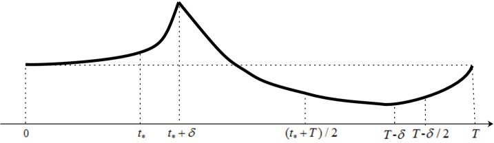
Figure 9. Profile of the function $\gamma$, which is illustrated by the black solid curve.

To verify that $\overline{\varphi}$ defined above is a super-solution satisfying (5.2), it remains to verify $\mathcal{L}_{\alpha}\overline{\varphi}\geq(\lambda^{*}-\epsilon)\overline{\varphi}$ in $(0,1)\times\left((0,T)\setminus\{t_{*},t_{*}+\delta\}\right)$. To this end, we divide the time interval $[0,T]$ into four parts: $\left[0,t_{*}\right]$, $\left[t_{*},t_{*}+\delta\right]$, $\left[t_{*}+\delta,T-\delta\right]$, and $[T-\delta,T]$.

Part 1. For $t\in\left[0,t_{*}\right]$, we choose $\gamma$ to satisfy

(5.7) $$\gamma^{\prime}(t)\geq 0,\quad\gamma(0)=1,\quad\gamma^{\prime}(0^{+})=0,\quad\gamma(t_{*})=1+\epsilon.$$

In view of $b(t)=0$, $\beta(x,t)=1$, and $\gamma^{\prime}(t)\geq 0\,\text{ in }\,[0,1]\times\left[0,t_{*}\right]$, we use (5.3) to calculate that

$$\mathcal{L}_{\alpha}\overline{\varphi} =\gamma\partial_{t}\psi^{*}+\gamma^{\prime}\psi^{*}-\gamma\partial_{xx}\psi^{*}+\gamma V(x,t)\psi^{*}$$

$$\geq\gamma(\partial_{t}\psi^{*}-\partial_{xx}\psi^{*}+V(x,t)\psi^{*})$$

$$=\lambda^{*}\gamma\psi^{*}>(\lambda^{*}-\epsilon)\overline{\varphi},\ \ \forall(x,t)\in[0,1]\times[0,t_{*}],$$

where the second equality is due to the definition of $\psi^{*}$ in (5.1).

Part 2. For $t\in\left(t_{*},t_{*}+\delta\right]$, we define

(5.8) $$\begin{array}[]{l}\gamma(t):=(1+\epsilon)e^{M_{\gamma}\left(t-t_{*}\right)},\end{array}$$

where $M_{\gamma}$ is defined in (5.6). Recall that for any fixed $t\in\left[t_{*},T\right]$, $\psi^{*}(\cdot,t)$ is a constant as noted in Remark 5.1. By direct calculation we have

$$\mathcal{L}_{\alpha}\overline{\varphi}=\gamma\beta\partial_{t}\psi^{*}+V(1,t)\gamma\beta\psi^{*}+\gamma^{\prime}\beta\psi^{*}+[\partial_{t}\beta-\partial_{xx}\beta-\alpha b\partial_{x}\beta+V(x,t)\beta-V(1,t)\beta]\gamma\psi^{*}.$$

Since $\partial_{x}\beta\leq 0$ and $|\partial_{t}\beta|,|\partial_{x}\beta|,|\partial_{xx}\beta|<M_{\beta}\beta$ on $[0,1]\times(t_{*},t_{*}+\delta]$, we deduce from (i) that

$$\mathcal{L}_{\alpha}\overline{\varphi} \geq\lambda^{*}\gamma\beta\psi^{*}+\gamma^{\prime}\beta\psi^{*}+[\partial_{t}\beta-\partial_{xx}\beta+V(x,t)\beta-V(1,t)\beta]\gamma\psi^{*}$$

$$\geq\lambda^{*}\overline{\varphi}+\gamma^{\prime}\beta\psi^{*}+[-2M_{\beta}+V(x,t)-V(1,t)]\gamma\beta\psi^{*}$$

$$=[\lambda^{*}-2M_{\beta}+V(x,t)-V(1,t)+M_{\gamma}]\overline{\varphi}$$

$$\geq(\lambda^{*}-\epsilon)\overline{\varphi},\ \ \forall(x,t)\in[0,1]\times(t_{*},t_{*}+\delta].$$

Part 3. For $t\in\left[t_{*}+\delta,T-\delta\right]$, we set

(5.9) $$\begin{cases}\gamma(t)=(1+\epsilon)e^{M_{\gamma}\delta}e^{-\frac{\epsilon}{Q}(t-t_{*}-\delta)}&\text{ on }\,\,\left[t_{*}+\delta,\frac{T+t_{*}}{2}\right],\\ -\frac{2\epsilon\gamma}{Q}<\gamma^{\prime}(t)<0,&\text{ on }\,\,\left(\frac{T+t_{*}}{2},T-\delta\right),\\ \gamma^{\prime}(T-\delta)=0,\end{cases}$$

where $M_{\gamma}$ and $Q$ are defined in (5.6). We then calculate that

(5.10) $$\begin{split}\mathcal{L}_{\alpha}\overline{\varphi}=\lambda^{*}\gamma\beta\psi^{*}+\gamma^{\prime}\beta\psi^{*}+[\partial_{t}\beta-\partial_{xx}\beta-\alpha b\partial_{x}\beta+V(x,t)\beta-V(1,t)\beta]\gamma\psi^{*}.\end{split}$$

Note that $\beta=1$ on $\{1\}\times\left[t_{*}+\delta,T\right]$. By taking $\delta$ small if necessary, we may assume

(5.11) $$|\partial_{t}\beta|+|\partial_{xx}\beta|<\tfrac{\epsilon}{3}\beta\quad\text{on}\ [1-2\delta,1]\times\left[t_{*}+\delta,T\right].$$

For $(x,t)\in[1-2\delta,1]\times\left[t_{*}+\delta,T-\delta\right]$, in view of $\partial_{x}\beta\leq 0$ and (ii), it follows from (5.10) that

$$\mathcal{L}_{\alpha}\overline{\varphi}\geq\lambda^{*}\overline{\varphi}+\gamma^{\prime}\beta\psi^{*}-\epsilon\gamma\beta\psi^{*}.$$

By the choice of $\gamma$ in (5.9), we arrive at

$$\mathcal{L}_{\alpha}\overline{\varphi}\geq\left(\lambda^{*}-\tfrac{(Q+2)\epsilon}{Q}\right)\overline{\varphi}.$$

For $(x,t)\in\left[0,1-2\delta\right]\times\left[t_{*}+\delta,T-\delta\right]$, by the conditions on $\beta$ and $b$, clearly there exists some constant $\rho>0$ independent of $(x,t)$ such that $b(t)\partial_{x}\beta(x,t)<-\rho$, whence by (5.10),

$$\begin{array}[]{l}\mathcal{L}_{\alpha}\overline{\varphi}\geq\left[\lambda^{*}\beta-\frac{2}{Q}\epsilon\beta-2M_{\beta}\beta+V(x,t)\beta-V(1,t)\beta+\alpha\rho\right]\gamma\psi^{*}.\end{array}$$

By choosing $\alpha$ large, we deduce $\mathcal{L}_{\alpha}\overline{\varphi}\geq(\lambda^{*}-\epsilon)\overline{\varphi}$ as desired.

Part 4. For $t\in\left[T-\delta,T\right]$, it can be observed from (5.6) and (iii) that

$$\gamma\left(\tfrac{T+t_{*}}{2}\right)=(1+\epsilon)e^{M_{\gamma}\delta}e^{-\frac{\epsilon}{Q}\left(\frac{T-t_{*}}{2}-\delta\right)}<e^{-\frac{M_{\gamma}\delta}{2}}=\gamma\left(T-\delta\right).$$

This allows us to define $\gamma$ as a smooth function on $(T-\delta,T]$ such that

(5.12) $$\gamma^{\prime}\geq 0\ \ \text{ on }(T-\delta,T-\tfrac{\delta}{2})\quad\text{and}\quad\gamma=e^{M_{\gamma}(t-T)}\,\,\text{ on }[T-\tfrac{\delta}{2},T].$$

To verify $\mathcal{L}_{\alpha}\overline{\varphi}\geq(\lambda^{*}-\epsilon)\overline{\varphi},$ we consider the following different regions.

For $(x,t)\in\left[1-2\delta,1\right]\times\left[T-\delta,T\right]$, by means of the facts $|\partial_{t}\beta|,|\partial_{xx}\beta|<\frac{\epsilon}{4}\beta$ in (5.11), $\partial_{x}\beta\leq 0$ and $\gamma^{\prime}(t)\geq 0$, we deduce from (5.10) and (ii) that

$$\begin{array}[]{l}\vskip 6.0pt plus 2.0pt minus 2.0pt\mathcal{L}_{\alpha}\overline{\varphi}\geq\lambda^{*}\gamma\beta\psi^{*}-\epsilon\gamma\beta\psi^{*}=(\lambda^{*}-\epsilon)\overline{\varphi}.\end{array}$$

For $(x,t)\in\left[0,1-2\delta\right]\times\left[T-\frac{\delta}{2},T\right]$, in view of $\partial_{x}\beta<0$ and $\gamma=e^{M_{\gamma}(t-T)}$, it follows from (5.10) and (i) that

$$\mathcal{L}_{\alpha}\overline{\varphi} \geq\lambda^{*}\gamma\beta\psi^{*}+\gamma^{\prime}\beta\psi^{*}+\left[\partial_{t}\beta-\partial_{xx}\beta+V(x,t)\beta-V(1,t)\beta\right]\gamma\psi^{*}$$

$$\geq\left[\lambda^{*}-2M_{\beta}+V(x,t)-V(1,t)+M_{\gamma}\right]\overline{\varphi}\geq(\lambda^{*}-\epsilon)\overline{\varphi}.$$

For $(x,t)\in\left[0,1-2\delta\right]\times\left[T-\delta,T-\frac{\delta}{2}\right]$, there exists some constant $\rho>0$ independent of $(x,t)$ such that $b(t)\partial_{x}\beta(x,t)<-\rho$ and $\gamma^{\prime}>0$. Noting that $|\partial_{t}\beta|,|\partial_{xx}\beta|<M_{\beta}\beta$, by choosing $\alpha$ to be large enough, we may use (5.10) to obtain

$$\mathcal{L}_{\alpha}\overline{\varphi} \geq\left[\lambda^{*}\beta-2M_{\beta}\beta+V(x,t)\beta-V(1,t)\beta+\alpha\rho\right]\gamma\psi^{*}\geq(\lambda^{*}-\epsilon)\overline{\varphi}.$$

By now, we have specified the function $\gamma$ through (5.7), (5.8), (5.9) and (5.12), which satisfies (5.4) and (5.5). Therefore, the super-solution $\overline{\varphi}$ constructed above satisfies (5.2), and thus $\liminf\limits_{\alpha\rightarrow\infty}\lambda(\alpha)\geq\lambda^{*}$ is established.

The proof of $\limsup\limits_{\alpha\rightarrow\infty}\lambda\leq\lambda^{*}$ is similar, which amounts to construct a sub-solution $\underline{\varphi}$ such that

(5.13) $$\begin{cases}\mathcal{L}_{\alpha}\underline{\varphi}\leq(\lambda^{*}+\epsilon)\underline{\varphi}&{\text{in}}\,\,(0,1)\times((0,T)\setminus\{t_{*},t_{*}+\delta\}),\\ \partial_{x}\underline{\varphi}(0,t)\geq 0,\ \ \partial_{x}\underline{\varphi}(1,t)\leq 0&{\text{on}}\,\,[0,T],\\ \underline{\varphi}(x,t_{*}^{+})<\underline{\varphi}(x,t_{*}^{-})&{\text{on}}\,\,(0,1),\\ \partial_{t}\overline{\varphi}(x,(t_{*}+\delta)^{-})<\partial_{t}\overline{\varphi}(x,(t_{*}+\delta)^{+})&{\text{on}}\,\,(0,1),\\ \underline{\varphi}(x,0)=\underline{\varphi}(x,T)&{\text{on}}\,\,(0,1),\end{cases}$$

where $\delta$ is given as before. Indeed, we can define

$$\underline{\varphi}(x,t):=\frac{\underline{\beta}(x,t)\psi^{*}}{\gamma(t)},$$

where $\gamma$ is defined as above and $\underline{\beta}>0$ has the same properties as $\beta$ except that $\partial_{x}\underline{\beta}>0$ on $[0,1)\times(t_{*},T)$. Proceeding as before, we can verify such a function $\underline{\varphi}$ is a strict sub-solution satisfying (5.13). Applying Proposition 2.1 again, we derive $\limsup_{\alpha\rightarrow\infty}\lambda(\alpha)\leq\lambda^{*}$. The proof is now completed. ∎

Next, we consider another typical function $b$.

Proposition 5.2.

Assume that the $T$-periodic function $b\in C(\mathbb{R})$ satisfies

$$b(t)>0\text{ in }(0,t_{*}),\quad b(t)<0\text{ in }(t_{*},T),\quad\text{and}\quad b(0)=b\left(t_{*}\right)=b(T)=0\quad{\text{f}or\ some}\ t_{*}\in(0,T).$$

Let $\lambda(\alpha)$ be the principal eigenvalue of (1.10). Then

$$\lim_{\alpha\rightarrow\infty}\lambda(\alpha)=\frac{1}{T}\left[\int^{t_{*}}_{0}V(1,s)\mathrm{d}s+\int^{T}_{t_{*}}V(0,s)\mathrm{d}s\right].$$

Proof.

Consider the following auxiliary eigenvalue problem:

(5.14) $$\left\{\begin{array}[]{ll}\frac{{\rm d}\psi}{{\rm d}t}+V(1,t)\psi=\lambda\psi&{\text{in}}\,\,\left(0,t_{*}\right],\\ \frac{{\rm d}\psi}{{\rm d}t}+V(0,t)\psi=\lambda\psi&{\text{in}}\,\,\left(t_{*},T\right],\\ \psi(t_{*}^{+})=\psi(t_{*}^{-}),\\ \psi(0)=\psi(T).\end{array}\right.$$

The existence of the principal eigenvalue, denoted by $\lambda^{**}$, of problem (5.14) is shown in Proposition A.1. It is easily seen that $\lambda^{**}=\frac{1}{T}\left[\int^{t_{*}}_{0}V(1,s)\mathrm{d}s+\int^{T}_{t_{*}}V(0,s)\mathrm{d}s\right].$ Define $\psi^{**}(t)>0$ as the corresponding principal eigenfunction of (5.14). Set

$$\overline{\varphi}(x,t):=\overline{\gamma}(t)\overline{\beta}(x,t)\psi^{**}(t).$$

Here $\overline{\beta}\in C^{1,1}([0,1]\times([0,t_{*})\cup(t_{*},T]))$ is chosen to be $T$-periodic and satisfies

$$\begin{cases}\overline{\beta}=1,\,\,\partial_{x}\overline{\beta}=0\ \ &\text{on}~{}(\{1\}\times(0,t_{*}))\cup(\{0\}\times(t_{*},T)),\\ \partial_{x}\overline{\beta}<0&\text{in}~{}[0,1)\times(0,t_{*}),\\ \partial_{x}\overline{\beta}>0&\text{in}~{}(0,1]\times(t_{*},T),\\ \overline{\beta}=1&\text{on}~{}[0,1]\times\{t_{*}\}.\end{cases}$$

Given $\delta>0$ to be determined later, the $T$-periodic function $\overline{\gamma}\in C([0,T])$ is chosen to be positive, smooth except for $t\in\{t_{*}\pm\delta,t_{*}\}$, and satisfy the following properties:

$$\begin{cases}\overline{\gamma}^{\prime}>0\ \ &\text{in}~{}\left[0,\delta\right)\cup\left(t_{*}-\delta,t_{*}+\delta\right)\cup\left(T-\delta,T\right],\\ \overline{\gamma}^{\prime}<0&\text{in}~{}\left(\delta,t_{*}-\delta\right)\cup\left(t_{*}+\delta,T-\delta\right),\\ \overline{\gamma}^{\prime}=0&\text{on}~{}\{\delta,T-\delta\},\end{cases}$$

and $\overline{\gamma}^{\prime}(T^{-})>\overline{\gamma}^{\prime}(0^{+})$ and $\overline{\gamma}^{\prime}(t^{-})>\overline{\gamma}^{\prime}(t^{+})$ for $t=t_{*}\pm\delta,\,t_{*}$.

Given any $\epsilon>0$, we can find suitable $\delta$, $\overline{\gamma}$ and $\overline{\beta}$ such that the above $\overline{\varphi}$ satisfies

$$\begin{cases}\mathcal{L}_{\alpha}\overline{\varphi}\geq(\lambda^{**}-\epsilon)\overline{\varphi}\ \ &{\text{in}}\,\,((0,1)\times[0,T])\setminus\mathbb{T},\\ \overline{\varphi}(x,t_{*}^{+})>\overline{\varphi}(x,t_{*}^{-})&{\text{on}}\,\,(0,1),\\ \partial_{t}\overline{\varphi}(x,t^{-})>\partial_{t}\overline{\varphi}(x,t^{+})&{\text{on}}\,\,(0,1)\times\{t_{*}-\delta,\,t_{*}+\delta\},\\ \partial_{x}\overline{\varphi}(0,t)\leq 0,\ \ \partial_{x}\overline{\varphi}(1,t)\geq 0&{\text{on}}\,\,[0,T],\\ \overline{\varphi}(x,0)=\overline{\varphi}(x,T)&{\text{on}}\,\,(0,1),\end{cases}$$

with $\mathbb{T}=[0,1]\times\{t_{*}\pm\delta,\,t_{*}\}$, provided that $\alpha$ is large enough. The process is a straightforward adaptation of the proof presented in parts $\mathbf{(2)}$-$\mathbf{(4)}$ of Proposition 5.1, and we omit the details. Consequently, applying Proposition 2.1 and letting $\epsilon\searrow 0$ give $\liminf_{\alpha\rightarrow\infty}\lambda(\alpha)\geq\lambda^{**}.$

The construction of a sub-solution $\underline{\varphi}$ follows from the same arguments as in Proposition 5.1 and thus $\limsup_{\alpha\rightarrow\infty}\lambda(\alpha)\leq\lambda^{**}.$ Proposition 5.2 is now proved. ∎

By a similar analysis to Proposition 5.2, we can also deduce the following result.

Proposition 5.3.

Assume that the $T$-periodic function $b\in C(\mathbb{R})$ satisfies

$$b(t)>0\ \ \text{ in }\,(0,t_{*})\cup(t_{*},T)\quad\text{and}\quad b\left(t_{*}\right)=0\quad{\text{f}or\ some}\ t_{*}\in(0,T).$$

Let $\lambda(\alpha)$ be the principal eigenvalue of (1.10). Then $\lambda(\alpha)\to\frac{1}{T}\int^{T}_{0}V(1,s)\mathrm{d}s$ as $\alpha\to\infty$.

Remark 5.2.

(1) The result parallel to Proposition 5.2 holds: Let $b$ satisfy

$$b(t)<0\text{ in }(0,t_{*}),\,\,b(t)>0\text{ in }(t_{*},T),\text{ and }b(0)=b\left(t_{*}\right)=b(T)=0\quad\text{for some}\ t_{*}\in(0,T).$$

Then the principal eigenvalue $\lambda(\alpha)$ of (1.10) satisfies

$$\lim_{\alpha\rightarrow\infty}\lambda(\alpha)=\frac{1}{T}\left[\int^{t_{*}}_{0}V(0,s)\mathrm{d}s+\int^{T}_{t_{*}}V(1,s)\mathrm{d}s\right].$$

This can be deduced by using the variable change $y=1-x$ in Proposition 5.2. Similarly, we can derive the results parallel to Propositions 5.1 and 5.3;

(2) In Proposition 5.1, the limit value $\lambda^{*}$ (of the principal eigenvalue as $\alpha\to\infty$) satisfies $\lambda^{*}\to\lambda^{\mathcal{N}\mathcal{N}}\big{(}(0,1)\big{)}$ as $t_{*}\nearrow T$ and $\lambda^{*}\to\frac{1}{T}\int^{T}_{0}V(1,s)\mathrm{d}s$ as $t_{*}\searrow 0$, which correspond to Proposition 4.1 and Remark 3.1, respectively;

(3) Proposition 5.3 suggests that when $b\geq\not\equiv 0$ or $b\leq\not\equiv 0$ on $[0,T]$, finitely many isolated critical points of $b$ will have no effects on the limit of $\lambda(\alpha)$ as $\alpha\rightarrow\infty$.

By the ideas developed in the proofs of Propositions 5.1 and 5.2, we can derive Theorem 1.3.

Proof of Theorem 1.3.

As before, it suffices to construct the suitable sub-solution and super-solution for (1.10) and apply Proposition 2.1. We shall follow the above arguments to construct a super-solution here and a sub-solution can be found similarly.

Let $\psi_{\infty}>0$ denote the principal eigenfunction of problem (1.11). Define

(5.15) $$\overline{\varphi}(x,t):=\gamma(t)\beta(x,t)\psi_{\infty}(x,t).$$

Following the proofs of Propositions 5.1 and 5.2, the $T$-periodic function $\beta$ is chosen to satisfy $\beta\in C^{1,1}([0,1]\times([0,T]\setminus\{t_{i},1\leq i\leq N\}))$ and

$$\begin{cases}\beta=1,\partial_{x}\beta=0,&\mathrm{on}~{}(\{1\}\times\left\{\left[t_{i},t_{i+1}\right],i\in\mathbb{C}\right\})\cup(\{0\}\times\left\{\left[t_{i},t_{i+1}\right],i\in\mathbb{A}\right\}),\\ \partial_{x}\beta<0&\text{on}~{}\left[0,1\right)\times\left\{\left[t_{i},t_{i+1}\right],i\in\mathbb{C}\right\},\\ \partial_{x}\beta>0&\text{on}~{}\left(0,1\right]\times\left\{\left[t_{i},t_{i+1}\right],i\in\mathbb{A}\right\},\\ \beta=1&\text{on}~{}\left[0,1\right]\times\left(\left\{\left[t_{i},t_{i+1}\right],i\in\mathbb{B}\right\}\cup\left\{t_{i},i\in\mathbb{A}\cup\mathbb{C}\right\}\right).\end{cases}$$

The $T$-periodic function $\gamma$ is assumed to be positive, continuous everywhere and satisfy that

$$\begin{cases}\gamma^{\prime}(t)\geq 0\ &\text{on}\,\left\{\left[t_{i},t_{i+1}\right],i\in\mathbb{B}\right\},\\ \gamma^{\prime}(t)>0&\text{on}\,\left\{\left(t_{i},t_{i}+\delta\right)\cup(t_{i+1}-\delta,t_{i+1}),i\in\mathbb{A}\cup\mathbb{C}\right\},\\ \gamma^{\prime}(t)<0&\text{on}\,\left\{\left(t_{i}+\delta,t_{i+1}\right),i\in\mathbb{A}\cup\mathbb{C}\right\},\end{cases}$$

and that for any $1\leq i\leq N+1$,

$$\gamma^{\prime}(t_{i+1}-\delta)=0,\quad\gamma^{\prime}(t_{i}^{-})>\gamma^{\prime}(t_{i}^{+}),\quad\text{and}\quad\gamma^{\prime}((t_{i}+\delta)^{-})>\gamma^{\prime}((t_{i}+\delta)^{+}).$$

Let $\mathbb{T}=(0,1)\times\{t_{i},t_{i}\pm\delta,1\leq i\leq N\}$. By the similar arguments as in Proposition 5.1, we can piecewise construct suitable $\gamma$ and $\beta$ on different intervals $[t_{i},t_{i+1}]$ ($0\leq i\leq N$) such that for small $\epsilon>0$, the chosen $\overline{\varphi}$ in (5.15) satisfies

$$\begin{cases}\mathcal{L}_{\alpha}\overline{\varphi}\geq(\lambda_{\infty}-\epsilon)\overline{\varphi}&{\rm{in}}\,\left((0,1)\times[0,T]\right)\setminus\mathbb{T},\\ \overline{\varphi}(x,t_{i}^{+})>\overline{\varphi}(x,t_{i}^{-})&{\text{on}}\,\,(0,1),\,1\leq i\leq N,\\ \partial_{t}\overline{\varphi}(x,t^{-})>\partial_{t}\overline{\varphi}(x,t^{+})&{\text{on}}\,\,(0,1)\times\{t_{i}\pm\delta,1\leq i\leq N\},\\ \partial_{x}\overline{\varphi}(0,t)\leq 0,\ \ \partial_{x}\overline{\varphi}(1,t)\geq 0&{\text{in}}\,[0,T],\\ \overline{\varphi}(x,0)=\overline{\varphi}(x,T)&{\text{in}}\,(0,1),\end{cases}$$

provided that $\alpha$ is sufficiently large. This implies that $\overline{\varphi}$ is a strict super-solution in the sense of Definition 2.1. Therefore, Theorem 1.3 follows from Proposition 2.1. ∎

Appendix A The existence of the principal eigenvalue of (1.11)

This section is devoted to the proof of the existence and uniqueness of the principal eigenvalue for problem (1.11), which is the limit value for $\lambda(\alpha)$ as $\alpha\to\infty$ under the assumption there.

Proposition A.1.

The problem (1.11) admits a unique principal eigenvalue $\lambda_{\infty}$ that corresponds to an eigenfunction $\psi$ satisfying

(A.1) $$\left\{\begin{array}[]{l}\vskip 6.0pt plus 2.0pt minus 2.0pt\psi>0\,\,\text{ in }\,[0,1]\times[0,T],\\ \psi\in C^{2+\sigma,1+\frac{\sigma}{2}}\left([0,1]\times([0,T]\setminus\{t_{1},\ldots,t_{N+1}\})\right)\,\text{ for some }\sigma\in(0,1).\end{array}\right.$$

Conversely, if (1.11) has a solution $\psi_{1}$ satisfying problem (A.1), then necessarily $\lambda=\lambda_{\infty}$ and $\psi_{1}=c\psi$ for some constant $c>0$.

Proof.

Our proof essentially adapts the ideas developed in [15, Theorem 3.4], which deals with an eigenvalue problem over a varying cylinder.

For any given $u_{0}(x,0)\in X:=\{w\in C^{1}([0,1]):w^{\prime}(0)=w^{\prime}(1)=0\}$, we define $u_{i}(x,t)$ ($1\leq i\leq N$) recursively as the unique solution of the problem

(A.2) $$\begin{cases}\left.\begin{array}[]{ll}\vskip 3.0pt plus 1.0pt minus 1.0pt\partial_{t}u_{i}+V(0,t)u_{i}=0&{\text{in}}\,\,(0,1)\times\left(t_{i},t_{i+1}\right],\\ u_{i}(x,t_{i}^{+})\equiv u_{i-1}(0,t_{i}^{-})&{\text{on}}\,\,(0,1),\\ \end{array}\right\}\ \,i\in\mathbb{A}\\ \left.\begin{array}[]{ll}\vskip 3.0pt plus 1.0pt minus 1.0pt\partial_{t}u_{i}-\partial_{xx}u_{i}+V(x,t)u_{i}=0&{\text{in}}\,\,(0,1)\times\left(t_{i},t_{i+1}\right],\\ u_{i}(x,t_{i}^{+})=u_{i-1}(x,t_{i}^{-})&{\text{on}}\,\,(0,1),\\ \end{array}\right\}\ \,i\in\mathbb{B}\\ \left.\begin{array}[]{ll}\vskip 3.0pt plus 1.0pt minus 1.0pt\partial_{t}u_{i}+V(1,t)u_{i}=0&{\text{in}}\,\,(0,1)\times\left(t_{i},t_{i+1}\right],\\ u_{i}(x,t_{i}^{+})\equiv u_{i-1}(1,t_{i}^{-})&{\text{on}}\,\,(0,1),\\ \end{array}\right\}\ \,i\in\mathbb{C}\\ \,\,\,\partial_{x}u_{i}(0,t)=\partial_{x}u_{i}(1,t)=0\ \ {\text{in}}\,\left[0,T\right],\end{cases}$$

where $0=t_{1}<t_{2}<\ldots<t_{N+1}=T$ and the sets $\mathbb{A},\mathbb{B},\mathbb{C}$ are given in Theorem 1.3. By the standard $L^{p}$-theory of parabolic equations [16], we know that

$$u_{i}\in C^{\sigma}\left((t_{i},t_{i+1}],W^{2,p}(0,1)\right)\cap C^{1+\sigma}\left((t_{i},t_{i+1}],L^{p}(0,1)\right)\,\,\text{ for some }\sigma>0.$$

We may choose $p$ large enough such that $W^{2,p}(0,1)$ is embedded into $C^{1}([0,1])$. Thus, $u_{i}(\cdot,t)\in X$ for any $t\in[0,T]$ and $1\leq i\leq N$.

Let $u_{0}$ and $u_{i}$ ($1\leq i\leq N$) be given above. Define the operator $K:X\rightarrow X$ by

$$Ku_{0}:=u_{N}(\cdot,T).$$

We use $P^{o}$ to denote the interior of $P$, a cone of nonnegative functions in $X$. Then it can be shown that the operator $K$ is linear, compact and strongly positive. This fact can be verified by a standard argument with the help of the regularity theory and the maximum principle for parabolic equations. We omit the details and refer to [15, Theorem 3.4].

By the above properties for $K$, it follows from the Krein-Rutman theorem [23] that the spectral radius $r(K)$ of $K$ is positive, and it corresponds to an eigenvector $u^{*}\in P^{o}$. Moreover, if $K\tilde{u}=\tilde{r}\tilde{u}$ for some $\tilde{u}\in P^{o}$, then necessarily $\tilde{r}=r(K)$ and $\tilde{u}=cu^{*}$ for some constant $c>0$.

Let $U:[0,1]\times[0,T]$ be given by

$$U(x,0)=u^{*}(x)\text{ in }[0,1]\quad\text{and}\quad U(x,t)=u_{i}(x,t)\text{ in }[0,1]\times(t_{i},t_{i+1}]\quad\text{ for }1\leq i\leq N,$$

where $u_{i}$ is defined by (A.2) with $u_{0}(x)=u^{*}(x)$. By definition, we have

$$U(\cdot,T)=Ku^{*}=r(K)u^{*}\,\text{ in }[0,1].$$

Set $\psi^{*}(x,t):=e^{\lambda_{\infty}t}U(x,t)$ with $\lambda_{\infty}=-\frac{1}{T}\ln r(K)$. Clearly, such a function $\psi^{*}$ satisfies (A.1) and $\psi^{*}(x,0)=\psi^{*}(x,T)$. Direct calculations give that $\psi^{*}$ verifies (1.11) with $\lambda=\lambda_{\infty}$, which proves the existence of the principal eigenvalue.

Conversely, if (1.11) has a solution $\psi_{1}$ satisfying (A.1), then let $\tilde{r}:=e^{-\lambda T}$ and $\tilde{u}(x,t):=e^{-\lambda t}\psi_{1}(x,t).$ It can be verified that $\tilde{u}(x,t)$ satisfies (A.2) with $u_{0}=\psi_{1}(\cdot,0)$, and furthermore

$$K\psi_{1}(\cdot,0)=\tilde{u}(\cdot,T)=e^{-\lambda T}\psi_{1}(\cdot,T)=\tilde{r}\psi_{1}(\cdot,0).$$

In view of $\psi_{1}(\cdot,0)\in P^{o}$, the Krein-Rutman theorem [23] implies that $\tilde{r}=r(K)$ and $\tilde{u}=cu^{*}$ for some constant $c>0$, whence $\lambda=\lambda_{\infty}$ and $\psi_{1}=c\psi$. The proof is thus complete. ∎

Appendix B Proof of (4.8)

Proof of (4.8).

Recall from (1.6) that $\lambda^{\mathcal{N}\mathcal{N}}\big{(}(\kappa_{0}-\delta,\kappa+\delta)\big{)}$ defines the principle eigenvalue of

$$\begin{cases}\mathcal{L}_{0}\psi:=\partial_{t}\psi-\partial_{xx}\psi+V\psi=\lambda\psi,\ \ &x\in(\kappa(t)-\delta,\kappa(t)+\delta),\,t\in(0,T),\\ \partial_{x}\psi(\kappa-\delta,t)=\partial_{x}\psi(\kappa+\delta,t)=0,&t\in\left[0,T\right],\\ \psi(x,0)=\psi(x,T),&x\in(\kappa(0)-\delta,\kappa(0)+\delta).\end{cases}$$

For any given $\epsilon>0$, we fix some $\delta_{*}=\delta_{*}(\epsilon)>0$ small such that $|V(x,t)-V\left(\kappa,t\right)|<\epsilon$ for all $x\in\left[\kappa(t)-\delta_{*},\kappa(t)+\delta_{*}\right]$ and $t\in[0,T]$. Define

$$\overline{\varphi}(t):=\exp\left[{-\int_{0}^{t}V\left(\kappa(s),s\right)\mathrm{d}s+{t\over T}\int_{0}^{T}V\left(\kappa(s),s\right)\mathrm{d}s}\right].$$

For any $0<\delta<\delta_{*}$ and $x\in\left(\kappa(t)-\delta,\kappa(t)+\delta\right)$, $t\in[0,T]$, direct calculation gives

$$\mathcal{L}_{0}\overline{\varphi}\leq\partial_{t}\overline{\varphi}-\partial_{xx}\overline{\varphi}+(V\left(\kappa(t),t\right)+\epsilon)\overline{\varphi}=\left[\frac{1}{T}\int_{0}^{T}V\left(\kappa(s),s\right)\mathrm{d}s+\epsilon\right]\overline{\varphi}$$

and

$$\mathcal{L}_{0}\overline{\varphi}\geq\partial_{t}\overline{\varphi}-\partial_{xx}\overline{\varphi}+(V\left(\kappa(t),t\right)-\epsilon)\overline{\varphi}=\left[\frac{1}{T}\int_{0}^{T}V\left(\kappa(s),s\right)\mathrm{d}s-\epsilon\right]\overline{\varphi}.$$

Since $\overline{\varphi}$ is $T$-periodic, we can apply Proposition 2.1 to deduce that for any $0<\delta<\delta_{*}$,

$$\int_{0}^{T}V\left(\kappa(s),s\right)\mathrm{d}s-\epsilon\leq\lambda^{\mathcal{N}\mathcal{N}}\big{(}(\kappa-\delta,\kappa+\delta)\big{)}\leq\frac{1}{T}\int_{0}^{T}V\left(\kappa(s),s\right)\mathrm{d}s+\epsilon.$$

Letting $\delta\searrow 0$ and then $\epsilon\searrow 0$ give (4.8). ∎

Acknowledgments. We sincerely thank the referees for their valuable suggestions which help improve the manuscript. SL was partially supported by the NSF of China (grant Nos. 1207011419 and 11571364). YL was partially supported by the NSF (grant No. DMS-1853561). RP was partially supported by NSF of China (grant No. 11671175). MZ was partially supported by the Nankai Zhide Foundation and NSF of China (No. 11971498).

References

- [1] I. Averill, K.-Y. Lam, Y. Lou, The role of advection in a two-species competition model: a bifurcation approach, Mem. Amer. Math. Soc. 245 (2017): 1161.
- [2] F. Belgacem, C. Cosner, The effects of dispersal along environmental gradients on the dynamics of populations in heterogeneous environment, Canadian Appl. Math. Quarterly 3 (1995) 379-397.
- [3] R.S. Cantrell, C. Cosner, Spatial Ecology via Reaction-Diffusion Equations. Series in Mathematical and Computational Biology, John Wiley and Sons, Chichester, UK, 2003.
- [4] R.S. Cantrell, C. Cosner, Evolutionary stability of ideal free dispersal under spatial heterogeneity and time periodicity, Math. Biosci. 305 (2018) 71-76.
- [5] R.S. Cantrell, C. Cosner, K.-Y. Lam, Ideal free dispersal under general spatial heterogeneity and time periodicity, SIAM J. Appl. Math. 81 (2021) 789-813.
- [6] R.S. Cantrell, C. Cosner, Y. Lou, Movement towards better environments and the evolution of rapid diffusion, Math. Biosci. 240 (2006) 199-214.
- [7] R.S. Cantrell, C. Cosner, Y. Lou, Advection-mediated coexistence of competing species, Proc. Roy. Soc. Edinburgh Sect. A 137 (2007) 497-518.
- [8] F. Caubet, T. Deheuvels, Y. Privat, Optimal location of resources for biased movement of species: the 1D case, SIAM J. Appl. Math. 77 (2017) 1876-1903.
- [9] X.F. Chen, Y. Lou, Principal eigenvalue and eigenfunctions of an elliptic operator with large advection and its application to a competition model, Indiana Univ. Math. J. 57 (2008) 627-658.
- [10] X.F. Chen, Y. Lou, Effects of diffusion and advection on the smallest eigenvalue of an elliptic operators and their applications, Indiana Univ. Math J. 60 (2012) 45-80.
- [11] C. Cosner, Reaction-diffusion-advection models for the effects and evolution of dispersal, Discrete Contin. Dyn. Syst. 34 (2014) 1701-1745.
- [12] D. Daners, C. Thornett, Periodic-parabolic eigenvalue problems with a large parameter and degeneration, J. Differential Equations 261 (2016) 273-295.
- [13] Y. Du, S.-B. Hsu, Concentration phenomena in a nonlocal quasi-linear problem modeling phytoplankton I: existence, SIAM J. Math. Anal. 40 (2008) 1419-1440.
- [14] Y. Du, S.-B. Hsu, Concentration phenomena in a nonlocal quasi-linear problem modeling phytoplankton II: limiting profile, SIAM J. Math. Anal. 40 (2008) 1441-1470.
- [15] Y. Du, R. Peng, The periodic logistic equation with spatial and temporal degeneracies, Trans. Amer. Math. Soc. 364 (2012) 6039-6070.
- [16] A. Friedman, Partial Differential Equations of Parabolic Type, Prentice-Hall, Englewood Cliffs, N.J., 1964.
- [17] F. Hamel, N. Nadirashvili, E. Russ, Rearrangement inequalities and applications to isoperimetric problems for eigenvalues, Ann. Math. 174 (2011) 647-755.
- [18] P. Hess, Periodic-parabolic Boundary Value Problems and Positivity, Pitman Res., Notes in Mathematics 247, Longman Sci. Tech., Harlow, 1991.
- [19] M. W. Hirsch, Stability and convergence in strongly monotone dynamical systems. J. Reine Angew. Math. 383 (1988), 1-53.
- [20] J. Huisman, P. van Oostveen, F.J. Weissing, Species dynamics in phytoplankton blooms: incomplete mixing and competition for light, Amer. Naturalist 154 (1999) 46-67.
- [21] V. Hutson, W. Shen, G.T. Vickers, Estimates for the principal spectrum point for certain time-dependent parabolic operators, Proc. Amer. Math. Soc. 129 (2000) 1669-1679.
- [22] V. Hutson, K. Michaikow, P. Poláčik, The evolution of dispersal rates in a heterogeneous time-periodic environment, J. Math. Biol. 43 (2001) 501-533.
- [23] M. G. Krein, M. A. Rutman, Linear Operators Leaving Invariant a Cone in a Banach Space, American Mathematical Society, New York, 1950.
- [24] K.-Y. Lam, S. Liu, Y. Lou, Selected topics on reaction-diffusion-advection models from spatial ecology, Math. Appl. Sci. Eng. 1 (2020) 150-180.
- [25] K.-Y. Lam, Y. Lou, Persistence, Competition and Evolution, book chapter, The Dynamics of Biological Systems, A. Bianchi, T. Hillen, M. Lewis, Y. Yi eds., Springer Verlag. 2019.
- [26] K.-Y. Lam, Y. Lou, Evolution of dispersal: ESS in spatial models, J. Math. Biol. 68 (2014) 851-877.
- [27] K.-Y. Lam, Y. Lou, Evolutionarily stable and convergent stable strategies in reaction-diffusion models for conditional dispersal, Bull. Math. Biol. 76 (2014) 261-291.
- [28] S. Liu, Y. Lou, A functional approach towards eigenvalue problems associated with incompressible flow, Discrete Cont. Dynam. Syst. 40 (2020) 3715-3736.
- [29] S. Liu, Y. Lou, Classifying the level set of principal eigenvalue for time-periodic parabolic operators and applications, Submitted, (2021).
- [30] S. Liu, Y. Lou, R. Peng, M. Zhou, Monotonicity of the principal eigenvalue for a linear time-periodic parabolic operator, Proc. Amer. Math. Soc. 47 (2019) 5291-5302.
- [31] S. Liu, Y. Lou, R. Peng, M. Zhou, Asymptotics of the principal eigenvalue for a linear time-periodic parabolic operator II: Small diffusion, Trans. Amer. Math. Soc. 374 (2021) 4895-4930.
- [32] Y. Lou, F. Lutscher, Evolution of dispersal in advective environments, J. Math Biol. 69 (2014) 1319-1342.
- [33] Y. Lou, P. Zhou, Evolution of dispersal in advective homogeneous environments: The effect of boundary conditions, J. Differential Equations 259 (2015) 141-171.
- [34] Y. Lou, X.-Q. Zhao, P. Zhou, Global dynamics of a Lotka-Volterre competition-diffusion-advection system in heterogeneous environments, J. Math. Pure. Appl. 121 (2019) 47-82.
- [35] M. Ma, C. Ou, Existence, uniqueness, stability and bifurcation of periodic patterns for a seasonal single phytoplankton model with self-shading effect, J. Differential Equations 263 (2017) 5630-5655.
- [36] I. Mazari, G. Nadin, Y. Privat. Shape optimization of a weighted two-phase Dirichlet eigenvalue, ArXiv preprint, 2020. https://arxiv.org/abs/2001.02958.
- [37] G. Nadin, The principal eigenvalue of a space-time periodic parabolic operator, Ann. Math. Pur. Appl. 188 (2009) 269-295.
- [38] G. Nadin, Some dependence results between the spreading speed and the coefficients of the space-time periodic Fisher-KPP equation, Eur. J. Appl. Math. 22 (2011) 169-185.
- [39] K. Nagahara, E. Yanagida, Maximization of the total population in a reaction-diffusion model with logistic growth, Calc. Var. Partial Differential Equations 57 (2018): 80.
- [40] W.-M. Ni, The Mathematics of Diffusion, CBMS-NSF Regional Conf. Ser. in Appl. Math. 82, SIAM, Philadelphia, 2011.
- [41] E. Pachepsky, F. Lutscher, R. Nisbet, M.A. Lewis, Persistence, spread and the drift paradox, Theor. Popul. Biol. 67 (2005) 61-73.
- [42] R. Peng, G. Zhang, M. Zhou, Asymptotic behavior of the principal eigenvalue of a linear second order elliptic operator with small/large diffusion coefficient, SIAM J. Math. Anal. 51 (2019) 4724-4753.
- [43] R. Peng, X.-Q. Zhao, Effects of diffusion and advection on the principal eigenvalue of a periodic-parabolic problem with applications, Calc. Var. Partial Diff. 54 (2015) 1611-1642.
- [44] R. Peng, X.-Q. Zhao, A nonlocal and periodic reaction-diffusion-advection model of a single phytoplankton species, J. Math. Biol. 72 (2016) 755-791.
- [45] R. Peng, M. Zhou, Effects of large degenerate advection and boundary conditions on the principal eigenvalue and its eigenfunction of a linear second order elliptic operator, Indiana Univ. Math J. 67 (2018) 2523-2568.
- [46] M.H. Protter, H.F. Weinberger, Maximum Principles in Differential Equations, 2nd ed., Springer-Verlag, Berlin, 1984.
- [47] N. Shigesada, A. Okubo, Analysis of the self-shading effect on algal vertical distribution in natural waters, J. Math. Biol. 12 (1981) 311-326.
- [48] D.C. Speirs, W.S.C. Gurney, Population persistence in rivers and estuaries, Ecology 82 (2001) 1219-1237.
- [49] O. Vasilyeva, F. Lutscher, Population dynamics in rivers: analysis of steady states, Can. Appl. Math. Quart. 18 (2011) 439-469.
- [50] W. Walter, A theorem on elliptic differential inequalities and applications to gradient bounds, Math. Z. 200 (1989) 293-299.
- [51] X.-Q. Zhao, P. Zhou, On a Lotka-Volterra competition model: the effects of advection and spatial variation, Calc. Var. Partial Differential Equations 55 (2016): 73.