The $1{:}2{:}4$ resonance in a particle chain

Abstract

We consider four masses in a circular configuration with nearest-neighbour interaction, generalizing the spatially periodic Fermi–Pasta–Ulam-chain where all masses are equal. We identify the mass ratios that produce the $1{:}2{:}4$ resonance — the normal form in general is non-integrable already at cubic order. Taking two of the four masses equal allows to retain a discrete symmetry of the fully symmetric Fermi–Pasta–Ulam-chain and yields an integrable normal form approximation. The latter is also true if the cubic terms of the potential vanish. We put these cases in context and analyse the resulting dynamics, including a detuning of the $1{:}2{:}4$ resonance within the particle chain.

Key words: Fermi-Pasta-Ulam chain; resonance; normal forms; integrability;

1 Introduction

The Fermi–Pasta–Ulam (fpu) chain is one of the paradigmatic examples of a Hamiltonian system, see [10, 6] and references therein. The Hamiltonian function is

$$H(p,q) \;\;=\;\;\sum_{j=1}^{N}\;\left(\frac{p_{j}^{2}}{2m}\,+\,V(q_{j+1}-q_{j})\right)$$ (1a)

with $$N m$$ the number of particles, mass  a positive constant and nearest-neighbour potential

$$V(z) \;\;=\;\;\frac{1}{2}z^{2}\;+\;\frac{\alpha}{3}z^{3}\;+\;\frac{\beta}{4}z^{4}\enspace.$$ (1b)

The potential $V$ can be extended to higher powers in $z$. In the literature separate attention is often paid to the $\alpha$–chain ($\beta=0$) and the $\beta$–chain ($\alpha=0$). As an extension of harmonic oscillator interaction the $\beta$–chain is slightly more natural.

The dynamics defined by the Hamiltonian function (1) is described by the equations of motion

$$\dot{q}_{j}\;=\;\frac{\partial H}{\partial p_{j}}\;=\;\frac{p_{j}}{m}\enspace,\quad\dot{p}_{j}\;=\;-\frac{\partial H}{\partial q_{j}}\;=\;V^{\prime}(q_{j+1}-q_{j})\,-\,V^{\prime}(q_{j}-q_{j-1})\enspace,\quad j=1,\ldots,N$$

for $N$ particles under the force $F=-V^{\prime}$. The convention $q_{N+1}:=q_{1}$ puts the $N$–degrees-of-freedom (dof) chain into a circular configuration, one also speaks of the spatially periodic fpu-chain. Using the diagonal $\mathbb{S}^{1}$–symmetry

$$\begin{array}[]{ccc}\mathbb{S}^{1}\times\mathbb{R}^{2N}&\longrightarrow&\mathbb{R}^{2N}\\ (\theta,p,q)&\mapsto&(p,(q_{j}+\theta)_{j})\end{array}$$ (2)

enables us to reduce the equations of motion, thereby fixing the value of the momentum mapping

$$(p,q)\;\;\mapsto\;\;\sum_{j=1}^{N}p_{j}$$

corresponding with the linear momentum integral. This leads to a Hamiltonian system with $N-1$ dof.

The initial interest in [9] was with large $N$, at that time $N=32$ or $N=64$, trying to confirm the ergodic hypothesis, see also [8]. After this failed — the numerical experiment [9] did not show equipartition of energy at low energy level but quite to the contrary recurrence phenomena — many papers appeared on the fpu-chain and also smaller values of $N$ were considered. Interestingly, for $N=3$ the reduced system in $N-1=2$ dof was shown in [10] to be equivalent to the paradigmatic Hénon–Heiles system [14], a $\mathbb{Z}_{3}$–symmetric unfolding of the $1{:}1$ resonance. Moreover, as shown in [16, 15] the $1{:}1$ resonance also governs the normal form approximations of the fpu-chains with $N\geq 4$ and their normal forms are all integrable. This puts the classical fpu-chain in the realm of Kolmogorov–Arnol’d–Moser (kam) theory where invariant maximal tori of the approximating normal form persist for the original system. The invariant tori obstruct or at least delay equipartition of energy, see also [19]. It turns out that such integrable approximations do also exist for the fpu-chain with alternating masses [11, 5], see in particular [4] where the case $m_{j}=1,m,1,m$ of four alternating masses is analysed.

1.1 Problem formulation

In the inhomogenous fpu-chain the masses of the oscillating particles introduced in the Hamiltonian (1a) are not required to be equal. We follow [3] and consider four masses $m_{1},\ldots,m_{4}$ for which the fourth and first mass are also subject to nearest-neighbour interaction, resulting in a spatially periodic fpu-chain. Having unequal masses yields $4$ extra parameters — next to the coefficients $\alpha,\beta$ of the potential for the nearest-neighbour interaction — which can be brought down to one extra parameter by restricting to mass ratios that produce the $1{:}2{:}4$ resonance. Indeed, from [3] we know that there are $12$ curves of mass ratios producing the $1{:}2{:}4$ resonance.

The analysis of the equations of motion is carried out by computing normal forms. The approximations obtained in this way are valid in a neighbourhood of the equilibrium. In our problem the origin of the phase space is a stable equilibrium and, as we shall see, typical error estimates depend on the size $\varepsilon$ of a neighbourhood of this equilibrium.

From the approximating normal forms of the Hamiltonian function we want to identify invariant manifolds and ideally integrability of the normal form system. In addition we look for periodic solutions on a given energy manifold, in some cases normal modes. We have to explain the terminology as there exists some confusion in the literature. In physics a normal mode was originally a continuation of linearized motion restricted to one of the co-ordinate planes. However, reductions and transformations of the positions and momenta mix the variables and the original simple notion of normal mode gets lost. In our terminology we will for instance for $n$ actions $\tau=\tau_{1},\ldots,\tau_{n}$ and corresponding $n$ angles $\phi$ call $\tau_{1}$ a normal mode if we have identified a continuation of a periodic solution of the normal form for which $\tau_{2}=\tau_{3}=\ldots=\tau_{n}=0$.

The $1{:}2{:}4$ resonance with $\alpha\neq 0$ has in general not an integrable normal form, see [7]. However, if two opposite masses in the periodic chain are equal, then exchanging these masses yields a $\mathbb{Z}_{2}$–symmetry that enforces the cubic terms in the normal form to vanish, whereas the quartic terms produce the first non-trivial normal form. The same happens for the $\beta$–chain where the third order terms (with coefficient $\alpha$) are already zero in the original system. Such fourth order normal form approximations are integrable. Interestingly, it turns out that while the quintic terms in the normal form vanish as well, higher order truncations (starting at order six) do break the integrability of the normal form. This yields four different timescales in the dynamics of these inhomogenous fpu-chains: the fast harmonic motions in $1{:}2{:}4$ resonance, the semi-slow motion of the first non-trivial normal form that can be reduced to $1$ dof, the slow motion of all higher order normal forms, which still can be reduced to $2$ dof and the exponentially slow motion in $3$ dof.

As mentioned before, the normal form approximations have validity near equilibrium, for the approximation theorems see [17]. Suppose we consider solutions on an energy manifold near a stable equilibrium as is the case in $N-1$ dof for the Hamiltonian reduced from (1). When considering solutions near a stable equilibrium it is natural to introduce a small positive parameter $\varepsilon$ and rescale $q=\varepsilon\bar{q}$, $p=\varepsilon\bar{p}$, divide the Hamiltonian by $\varepsilon^{2}$ and leave out the bars. In the equations of motion this produces $\varepsilon\alpha,\varepsilon^{2}\beta$ instead of $\alpha,\beta$. The normalisation procedure keeps the quadratic part $H_{2}$ of the Hamiltonian (1) as an integral of the normal form equations.

A general result for time-independent Hamiltonians is that when normalising and using the cubic terms of the Hamiltonian, the solutions and integrals produce approximations with error $O(\varepsilon)$ valid on the timescale $1/\varepsilon$. In our special problem where the cubic terms vanish after the normalising transformation, the error estimate, when including the normalised quartic terms, is $O(\varepsilon^{2})$ valid on the timescale $1/\varepsilon^{2}$.

The same estimates hold for integral manifolds of normalised systems, but with a difference: they represent structures that are asymptotic approximations of phantom structures in the original system. For the normal form integral $H_{2}$ the timescale of validity can be extended, the approximation is valid for all time as the solutions in a neighbourhood of equilibrium are bounded. When including detuning effects, the approximation approach sketched here enables us to determine the size of the detuning parameters. When retaining nontrivial cubic terms they have to be of size $O(\varepsilon)$; if the normalised cubic terms vanish, the detuning is bounded by $O(\varepsilon^{2})$.

1.2 Plan of the paper

In the next section we formulate the inhomogenous fpu-chain in more detail, determine the masses that produce the $1{:}2{:}4$ resonance and reduce the $\mathbb{S}^{1}$–symmetry (2) of rotating the circular chain to arrive at our system in $3$ dof; classically this means that we use an integral independent of the energy to remove $1$ dof of the $4$–particles system. Section 3 then concerns the technical analysis of determining basic invariants to obtain the normal forms of the $1{:}2{:}4$ resonance. In section 4 we identify the cases with two equal masses, next to the $\beta$–chain the focus of this paper. A useful reduction to a $1$ dof problem is analysed in section 5. Section 6 is about the non-integrable higher order terms for $2$ dof and the implications for $3$ dof; we conclude with section 7.

2 The inhomogenous fpu-chain

For the inhomogeneous fpu-chain we allow the $4$ particle masses $m_{j}$ to be different. In the Hamiltonian (1a) we take $N=4$ and obtain

$$H(p,q)\;\;=\;\;\sum_{j=1}^{4}\;\left(\frac{p_{j}^{2}}{2m_{j}}\,+\,V(q_{j+1}-q_{j})\right)$$ (3)

while we keep the potential $V$ defined in (1b). We can write the quadratic part of $H(p,q)$ as

$$H_{2}\;\;=\;\;\frac{1}{2}p^{T}A_{4}p\;+\;\frac{1}{2}q^{T}C_{4}q$$ (4)

with $A_{4}={\mathop{\rm diag}}(\mu_{1},\ldots,\mu_{4})$ the $4\times 4$ diagonal matrix that has at position $(j,j)$ the inverse masses $m_{j}^{-1}=:\mu_{j}$ while the $4\times 4$ matrix

$$C_{4}\;\;=\;\;\left(\begin{array}[]{cccc}2&-1&0&-1\\ -1&2&-1&0\\ 0&-1&2&-1\\ -1&0&-1&2\end{array}\right)$$

encodes the quadratic part of the potential $V$. As shown in [3] one of the eigenvalues of $A_{4}C_{4}$ vanishes, corresponding to the $\mathbb{S}^{1}$–symmetry (2) and leading to the linear momentum integral, while the three remaining eigenvalues $\gamma_{1},\gamma_{2},\gamma_{3}$ of $A_{4}C_{4}$ put the restrictions

$$4(\mu_{1}+\mu_{3})\mu_{2}\mu_{4}\;+\;4(\mu_{2}+\mu_{4})\mu_{1}\mu_{3} = \gamma_{1}\gamma_{2}\gamma_{3}\;$$ (5a)

$$3(\mu_{1}+\mu_{3})(\mu_{2}+\mu_{4})\;+\;4(\mu_{1}\mu_{3}+\mu_{2}\mu_{4}) = \gamma_{1}\gamma_{2}\;+\;\gamma_{2}\gamma_{3}\;+\;\gamma_{1}\gamma_{3}$$ (5b)

$$2(\mu_{1}+\mu_{2}+\mu_{3}+\mu_{4}) = \gamma_{1}\;+\;\gamma_{2}\;+\;\gamma_{3}$$ (5c)

on the inverse masses $\mu_{j}$. Correspondingly, choices of the $\mu_{j}$ exist that produce the first order resonances $1{:}2{:}1$, $1{:}2{:}3$ and $1{:}2{:}4$ (but not $1{:}2{:}2$). The resulting $1{:}2{:}3$ resonance has been studied in [3], here we consider the $1{:}2{:}4$ resonance. Scaling to $\gamma_{1}+\gamma_{2}+\gamma_{3}+\gamma_{4}=21$ we have $\gamma_{1}=1$, $\gamma_{2}=4$ and $\gamma_{3}=16$ next to $\gamma_{4}=0$ whence the right hand side $\gamma_{1}\gamma_{2}\gamma_{3}$ of eq. (5a) becomes $64$ and the right hand side of eq. (5b) becomes $84$. We use $\mu_{2}+\mu_{4}=:v$ to parametrise the solutions $(\mu_{1},\mu_{2},\mu_{3},\mu_{4})\in\mathbb{R}^{4}_{>0}$ and first note that $v\neq\frac{21}{4}$. Indeed otherwise also $\mu_{1}+\mu_{3}=\frac{21}{4}$ by eq. (5c), whence $\mu_{1}\mu_{3}+\mu_{2}\mu_{4}=\frac{21}{64}$ by eq. (5b) and $\mu_{1}\mu_{3}+\mu_{2}\mu_{4}=\frac{64}{21}$ by eq. (5a) contradict each other. Then the solution of these equations is

$$\mu_{1,3} = \frac{21-2v\pm\sqrt{\Delta}}{4}$$

$$\mu_{2,4} = \frac{v\pm\sqrt{\Gamma}}{2}$$

where

$$\Delta = -\frac{(2v+11)(2v-19)(2v-13)}{4v-21}$$

$$\Gamma = -\frac{2(v-16)(v-4)(v-1)}{4v-21}\enspace.$$

Diagonalising $A_{4}^{\frac{1}{2}}C_{4}A_{4}^{\frac{1}{2}}=U\Lambda U^{T}$, $\Lambda={\mathop{\rm diag}}(\gamma_{1},\gamma_{2},\gamma_{3},0)$ with an orthogonal matrix $U$ yields the symplectic transformation

$$p\;=\;Ky\enspace,\quad q\;=\;Lx$$ (6)

adapted from [3] where

$$K\;=\;A_{4}^{-\frac{1}{2}}U\Omega^{\frac{1}{4}}\quad\mbox{and}\quad L\;=\;A_{4}^{\frac{1}{2}}U\Omega^{-\frac{1}{4}}$$

with $\Omega={\mathop{\rm diag}}(\gamma_{1},\gamma_{2},\gamma_{3},1)$ that turns the quadratic part (4) of the Hamiltonian (3) into

$$H_{2}\;\;=\;\;\sum_{j=1}^{3}2^{j-1}(\frac{x_{j}^{2}+y_{j}^{2}}{2})\;+\;\frac{y_{4}^{2}}{2}\enspace.$$ (7)

This simultaneously achieves two goals. On one hand the $\mathbb{S}^{1}$–action of eq. (2) becomes $x_{4}\mapsto x_{4}+\vartheta$, i.e. $x_{4}$ is a cyclic angle and reducing this $\mathbb{S}^{1}$–symmetry amounts to fixing the value $y_{4}$ of the momentum integral and ignoring the cyclic angle $x_{4}$, whence the reduced Hamiltonian in $3$ dof reads as

$$H_{2}\;\;=\;\;\frac{x_{1}^{2}+y_{1}^{2}}{2}\;+\;2(\frac{x_{2}^{2}+y_{2}^{2}}{2})\;+\;4(\frac{x_{3}^{2}+y_{3}^{2}}{2})\enspace.$$ (8)

On the other hand the transformation (6) achieves the splitting of the quadratic part of the reduced Hamiltonian into the three oscillators in $1{:}2{:}4$ resonance visible in eq. (8). For inverse masses $\mu_{j}$ that do not lead to resonant oscillators, this same procedure — with adapted $\Lambda$ and $\Omega$ — leads to the deformation

$$H_{2}^{\lambda}\;\;=\;\;(1+\lambda_{1})\frac{x_{1}^{2}+y_{1}^{2}}{2}\;+\;(2+\lambda_{2})\frac{x_{2}^{2}+y_{2}^{2}}{2}\;+\;(4+\lambda_{3})\frac{x_{3}^{2}+y_{3}^{2}}{2}$$ (9)

of the $1{:}2{:}4$ resonant oscillator (8), with detunings $\lambda_{j}=\lambda_{j}(\mu)$, $j=1,2,3$. This is the quadratic part of

$$H^{\lambda}(x,y)\;\;=\;\;H(Ky,Lx)$$ (10)

reduced from (3). As we have discussed in section 1.1, the detunings $\lambda_{1},\lambda_{2},\lambda_{3}$ depend in size on the order of the first non-zero terms in the normal form.

3 Harmonic and nonlinear oscillators in $1{:}2{:}4$ resonance

It is well-known that the flow induced by the quadratic Hamiltonian (8) is periodic and a truncated normal form of the Hamiltonian (10) with respect to (8) depends on $x,y$ only through certain invariants, see below (for the general theory see also chs. 11–13 in [17]). This allows to use the periodic flow of $X_{\textstyle\!\mbox{\small$H_{2}^{0}$}}$ to reduce to $2$ dof.

This embeds the reduced system into the space of invariants $\mathbb{R}^{11}$ where $11$ is the number of independent invariants, see below. However, as the $11\times 11$ Poisson matrix of these invariants has rank $4$, this is indeed a reduction from $3$ to $2$ dof (the Hamiltonian (8) acts as a Casimir). The effectiveness of determining invariants becomes clear in section 3.2 where we formulate the normalised equations of motion.

Note that a preliminary study of the Hamiltonian (10) at $\lambda=0$ is contained in [1], for a summary see [17]. We will pursue the study of such non-integrable normal forms in a subsequent paper. As shown in [7] already the general third order normal form of the $1{:}2{:}4$ resonance is not integrable.

In case there does exist a third independent integral (next to the quadratic (8) and the Hamiltonian itself) the normalised system is integrable and we can reduce to $1$ dof. As noted in [17] this may happen if there are additional discrete symmetries. Such a discrete symmetry is introduced if two opposite masses are equal as one then can flip the periodic chain about the other two masses without changing the equations of motion.

3.1 Invariants, syzygies and Poisson bracket relations

In complex co-ordinates $z_{k}=x_{k}+{\rm i}y_{k}$ the flow defined by $H_{2}^{0}$ reads as

$$(t,z)\;\;\mapsto\;\;\left({\rm e}^{-{\rm i}t}z_{1},{\rm e}^{-2{\rm i}t}z_{2},{\rm e}^{-4{\rm i}t}z_{3}\right)$$

whence a monomial $z_{1}^{m_{1}}z_{2}^{m_{2}}z_{3}^{m_{3}}\bar{z}_{1}^{n_{1}}\bar{z}_{2}^{n_{2}}\bar{z}_{3}^{n_{3}}$ is invariant if and only if $m_{1}+2m_{2}+4m_{3}=n_{1}+2n_{2}+4n_{3}$. The ring of functions invariant under this flow is generated by the basic invariants

$$\tau_{1} = \frac{1}{2}z_{1}\bar{z}_{1}\;\;=\;\;\frac{x_{1}^{2}+y_{1}^{2}}{2}$$

$$\tau_{2} = \frac{1}{2}z_{2}\bar{z}_{2}\;\;=\;\;\frac{x_{2}^{2}+y_{2}^{2}}{2}$$

$$\tau_{3} = \frac{1}{2}z_{3}\bar{z}_{3}\;\;=\;\;\frac{x_{3}^{2}+y_{3}^{2}}{2}$$

of degree $2$, the basic invariants

$$\sigma_{1} = \frac{1}{2}{\mathop{\rm Re}}\,z_{1}^{2}\bar{z}_{2}\;\;=\;\;\frac{x_{1}^{2}x_{2}+2x_{1}y_{1}y_{2}-x_{2}y_{1}^{2}}{2}$$

$$\sigma_{2} = \frac{1}{2}{\mathop{\rm Im}}\,z_{1}^{2}\bar{z}_{2}\;\;=\;\;\frac{y_{1}^{2}y_{2}+2x_{1}x_{2}y_{1}-x_{1}^{2}y_{2}}{2}$$

$$\sigma_{3} = \frac{1}{2}{\mathop{\rm Re}}\,z_{2}^{2}\bar{z}_{3}\;\;=\;\;\frac{x_{2}^{2}x_{3}+2x_{2}y_{2}y_{3}-x_{3}y_{2}^{2}}{2}$$

$$\sigma_{4} = \frac{1}{2}{\mathop{\rm Im}}\,z_{2}^{2}\bar{z}_{3}\;\;=\;\;\frac{y_{2}^{2}y_{3}+2x_{2}x_{3}y_{2}-x_{2}^{2}y_{3}}{2}$$

of degree $3$, the basic invariants

$$\sigma_{5} = \frac{1}{2}{\mathop{\rm Re}}\,z_{1}^{2}z_{2}\bar{z}_{3}\;\;=\;\;\frac{x_{1}^{2}(x_{2}x_{3}+y_{2}y_{3})\,+\,2x_{1}y_{1}(x_{2}y_{3}-x_{3}y_{2})\,-\,y_{1}^{2}(x_{2}x_{3}+y_{2}y_{3})}{2}$$

$$\sigma_{6} = \frac{1}{2}{\mathop{\rm Im}}\,z_{1}^{2}z_{2}\bar{z}_{3}\;\;=\;\;\frac{-x_{1}^{2}(x_{2}y_{3}-x_{3}y_{2})\,+\,2x_{1}y_{1}(x_{2}x_{3}+y_{2}y_{3})\,+\,y_{1}^{2}(x_{2}y_{3}-x_{3}y_{2})}{2}$$

of degree $4$ and the basic invariants

$$\sigma_{7} = \frac{1}{24}{\mathop{\rm Re}}\,z_{1}^{4}\bar{z}_{3}\;\;=\;\;\frac{(x_{1}^{4}-6x_{1}^{2}y_{1}^{2}+y_{1}^{4})x_{3}\,+\,4(x_{1}^{2}-y_{1}^{2})x_{1}y_{1}y_{3}}{24}$$

$$\sigma_{8} = \frac{1}{24}{\mathop{\rm Im}}\,z_{1}^{4}\bar{z}_{3}\;\;=\;\;\frac{4(x_{1}^{2}-y_{1}^{2})x_{1}x_{3}y_{1}\,-\,(x_{1}^{4}-6x_{1}^{2}y_{1}^{2}+y_{1}^{4})y_{3}}{24}$$

of degree $5$.

table Poisson brackets $\{\tau_{i},\sigma_{j}\}$ $\{\downarrow,\rightarrow\}$ $\sigma_{1}$ $\sigma_{2}$ $\sigma_{3}$ $\sigma_{4}$ $\sigma_{5}$ $\sigma_{6}$ $\sigma_{7}$ $\sigma_{8}$ $\tau_{1}$ $-2\sigma_{2}$ $2\sigma_{1}$ $0$ $0$ $-2\sigma_{6}$ $2\sigma_{5}$ $-4\sigma_{8}$ $4\sigma_{7}$ $\tau_{2}$ $\sigma_{2}$ $-\sigma_{1}$ $-2\sigma_{4}$ $2\sigma_{3}$ $-\sigma_{6}$ $\sigma_{5}$ $0$ $0$ $\tau_{3}$ $0$ $0$ $\sigma_{4}$ $-\sigma_{3}$ $\sigma_{6}$ $-\sigma_{5}$ $\sigma_{8}$ $-\sigma_{7}$

These $11$ basic invariants are not free, but restricted by the syzygies $S_{j}=0$, $j=1,\ldots,20$ given by

$$S_{1} = \frac{1}{2}(\sigma_{1}^{2}+\sigma_{2}^{2})\;-\;\tau_{1}^{2}\tau_{2}$$

$$S_{2} = \frac{1}{2}(\sigma_{3}^{2}+\sigma_{4}^{2})\;-\;\tau_{2}^{2}\tau_{3}$$

$$S_{3} = \sigma_{1}\sigma_{3}-\sigma_{2}\sigma_{4}\;-\;\tau_{2}\sigma_{5}$$

$$S_{4} = \sigma_{2}\sigma_{3}+\sigma_{1}\sigma_{4}\;-\;\tau_{2}\sigma_{6}$$

$$S_{5} = \sigma_{1}\sigma_{5}+\sigma_{2}\sigma_{6}\;-\;2\tau_{1}^{2}\sigma_{3}$$

$$S_{6} = \sigma_{1}\sigma_{6}-\sigma_{2}\sigma_{5}\;-\;2\tau_{1}^{2}\sigma_{4}$$

$$S_{7} = \sigma_{1}\sigma_{5}-\sigma_{2}\sigma_{6}\;-\;12\tau_{2}\sigma_{7}$$

$$S_{8} = \sigma_{2}\sigma_{5}+\sigma_{1}\sigma_{6}\;-\;12\tau_{2}\sigma_{8}$$

$$S_{9} = \sigma_{3}\sigma_{5}+\sigma_{4}\sigma_{6}\;-\;2\tau_{2}\tau_{3}\sigma_{1}$$

$$S_{10} = \sigma_{3}\sigma_{6}-\sigma_{4}\sigma_{5}\;-\;2\tau_{2}\tau_{3}\sigma_{2}$$

$$S_{11} = \frac{1}{4}(\sigma_{5}^{2}+\sigma_{6}^{2})\;-\;\tau_{1}^{2}\tau_{2}\tau_{3}$$

$$S_{12} = 6(\sigma_{1}\sigma_{7}+\sigma_{2}\sigma_{8})\;-\;\tau_{1}^{2}\sigma_{5}$$

$$S_{13} = 6(\sigma_{1}\sigma_{8}-\sigma_{2}\sigma_{7})\;-\;\tau_{1}^{2}\sigma_{6}$$

$$S_{14} = 6(\sigma_{3}\sigma_{7}-\sigma_{4}\sigma_{8})\;-\;\frac{1}{2}(\sigma_{5}^{2}-\sigma_{6}^{2})$$

$$S_{15} = 6(\sigma_{3}\sigma_{8}+\sigma_{4}\sigma_{7})\;-\;\sigma_{5}\sigma_{6}$$

$$S_{16} = 3(\sigma_{3}\sigma_{7}+\sigma_{4}\sigma_{8})\;-\;\frac{1}{2}\tau_{3}(\sigma_{1}^{2}-\sigma_{2}^{2})$$

$$S_{17} = 3(\sigma_{3}\sigma_{8}-\sigma_{4}\sigma_{7})\;-\;\tau_{3}\sigma_{1}\sigma_{2}$$

$$S_{18} = 3(\sigma_{5}\sigma_{7}+\sigma_{6}\sigma_{8})\;-\;\tau_{1}^{2}\tau_{3}\sigma_{1}$$

$$S_{19} = 3(\sigma_{5}\sigma_{8}-\sigma_{6}\sigma_{7})\;-\;\tau_{1}^{2}\tau_{3}\sigma_{2}$$

$$S_{20} = 18(\sigma_{7}^{2}+\sigma_{8}^{2})\;-\;\tau_{1}^{4}\tau_{3}$$

and by the inequalities $\tau_{1}\geq 0$, $\tau_{2}\geq 0$, $\tau_{3}\geq 0$. Note that the syzygies themselves have to satisfy (at least) $14$ relations. The Poisson bracket relations between the basic invariants are

$$\{\tau_{i},\tau_{j}\}\;\;=\;\;0\enspace,\quad i,j\;=\;1,2,3$$

while the $\{\tau_{i},\sigma_{j}\}$, $i=1,2,3$, $j=1,\ldots,8$ are given in table 3.1. The relations $\{\sigma_{i},\sigma_{j}\}$, $i,j=1,\ldots,8$ are split into tables 3.1 and 3.1 (here we use that $\{\sigma_{i},\sigma_{j}\}=-\{\sigma_{j},\sigma_{i}\}$).

table Poisson brackets $\{\sigma_{i},\sigma_{j}\}$ $\{\downarrow,\rightarrow\}$ $\sigma_{1}$ $\sigma_{2}$ $\sigma_{3}$ $\sigma_{4}$ $\sigma_{1}$ $0$ $-\tau_{1}(\tau_{1}-4\tau_{2})$ $-\sigma_{6}$ $\sigma_{5}$ $\sigma_{2}$ $\tau_{1}(\tau_{1}-4\tau_{2})$ $0$ $\sigma_{5}$ $\sigma_{6}$ $\sigma_{3}$ $\sigma_{6}$ $-\sigma_{5}$ $0$ $-\tau_{2}(\tau_{2}-4\tau_{3})$ $\sigma_{4}$ $-\sigma_{5}$ $-\sigma_{6}$ $\tau_{2}(\tau_{2}-4\tau_{3})$ $0$ $\sigma_{5}$ $4\tau_{1}\sigma_{4}+6\sigma_{8}$ $4\tau_{1}\sigma_{3}-6\sigma_{7}$ $-\sigma_{2}(\tau_{2}-2\tau_{3})$ $-\sigma_{1}(\tau_{2}-2\tau_{3})$ $\sigma_{6}$ $-4\tau_{1}\sigma_{3}-6\sigma_{7}$ $4\tau_{1}\sigma_{4}-6\sigma_{8}$ $\sigma_{1}(\tau_{2}-2\tau_{3})$ $-\sigma_{2}(\tau_{2}-2\tau_{3})$ $\sigma_{7}$ $\frac{2}{3}\tau_{1}\sigma_{6}$ $\frac{2}{3}\tau_{1}\sigma_{5}$ $-\frac{1}{6}\sigma_{1}\sigma_{2}$ $-\frac{1}{12}(\sigma_{1}^{2}-\sigma_{2}^{2})$ $\sigma_{8}$ $-\frac{2}{3}\tau_{1}\sigma_{5}$ $\frac{2}{3}\tau_{1}\sigma_{6}$ $\frac{1}{12}(\sigma_{1}^{2}-\sigma_{2}^{2})$ $-\frac{1}{6}\sigma_{1}\sigma_{2}$

The Poisson bracket relations together with the syzygies allow to identify the subsets $\{\tau_{1}=0\}$ and $\{\tau_{1}>0\}$ of the reduced phase space that are invariant under the dynamics for every Hamiltonian function $\mathcal{H}$ that can be written in terms of the invariants, in particular for truncated normal forms. Indeed, for $\tau_{1}=0$ the syzygies $S_{1}$, $S_{11}$ and $S_{20}$ enforce $\sigma_{1}=\sigma_{2}=\sigma_{5}=\sigma_{6}=\sigma_{7}=\sigma_{8}=0$ whence

$$\dot{\tau}_{1}\;\;=\;\;-2\sigma_{2}\frac{\partial\mathcal{H}}{\partial\sigma_{1}}\;+\;2\sigma_{1}\frac{\partial\mathcal{H}}{\partial\sigma_{2}}\;-\;2\sigma_{6}\frac{\partial\mathcal{H}}{\partial\sigma_{5}}\;+\;2\sigma_{5}\frac{\partial\mathcal{H}}{\partial\sigma_{6}}\;-\;4\sigma_{8}\frac{\partial\mathcal{H}}{\partial\sigma_{7}}\;+\;4\sigma_{7}\frac{\partial\mathcal{H}}{\partial\sigma_{8}}\;\;=\;\;0$$

and similarly $\dot{\sigma}_{1}=\dot{\sigma}_{2}=\dot{\sigma}_{5}=\dot{\sigma}_{6}=\dot{\sigma}_{7}=\dot{\sigma}_{8}=0$ — independent of $\mathcal{H}$ — ensure that the values of these invariants, in particular of $\tau_{1}$, stay zero. This makes the complement $\{\tau_{1}>0\}$ an invariant set as well.

This does not work for $\tau_{2}=0$ because of the $\tau_{1}^{2}$–contribution from $\{\sigma_{1},\sigma_{2}\}$ which furthermore prevents equilibria inside $\{\tau_{2}=0,\tau_{1}>0\}$. Even if $\mathcal{H}$ is independent of $\sigma_{1}$ and $\sigma_{2}$ there are non-zero terms in e.g. the brackets $\{\sigma_{1},\sigma_{5}\}$, $\{\sigma_{5},\sigma_{6}\}$ and $\{\sigma_{7},\sigma_{8}\}$. Similarly for $\tau_{3}=0$ because of the $\tau_{2}^{2}$–contribution from $\{\sigma_{3},\sigma_{4}\}$, also preventing equilibria inside $\{\tau_{3}=0,\tau_{1}>0\}$.

Furthermore this shows that the normal–$1$–mode $(\tau,\sigma)=(\tau_{1},0,\ldots,0)$ is not automatically an equilibrium; similarly for the normal–$2$–mode $(\tau,\sigma)=(0,\tau_{2},0,\ldots,0)$. However, the normal–$3$–mode $(\tau,\sigma)=(0,0,\tau_{3},0,\ldots,0)$ makes all Poisson brackets vanish, whence it is an equilibrium for every Hamiltonian function. This can also be obtained from the dynamics on the invariant set $\{\tau_{1}=0\}$, which is best understood by intersecting the energy level set with the surface of revolution

$$\sigma_{3}^{2}\;+\;\sigma_{4}^{2}\;\;=\;\;\tau_{2}^{2}\,(\eta-\tau_{2})\enspace,\quad 0\leq\tau_{2}\leq\eta$$

defined by the syzygy $S_{2}=0$. Here $\eta\geq 0$ is the value of the conserved quantity $\frac{1}{2}H_{2}^{0}$, allowing to replace $\tau_{3}$ by $\frac{1}{2}(\eta-\tau_{2})$ since $\tau_{1}=0$. The two surfaces touch in (regular) equilibria, while the singular point $\tau_{2}=0$ — the normal $3$–mode — is always an equilibrium.

table Poisson brackets $\{\sigma_{i},\sigma_{j}\}$ (continued) $\{\downarrow,\rightarrow\}$ $\sigma_{5}$ $\sigma_{6}$ $\sigma_{7}$ $\sigma_{8}$ $\sigma_{5}$ $0$ $\!\!\!\!\!\!\!\!-2\tau_{1}(\tau_{1}\tau_{2}-\tau_{1}\tau_{3}-4\tau_{2}\tau_{3})$ $\frac{1}{6}\tau_{1}\sigma_{2}(\tau_{1}-8\tau_{3})$ $-\frac{1}{6}\tau_{1}\sigma_{1}(\tau_{1}-8\tau_{3})$ $\sigma_{6}$ $2\tau_{1}(\tau_{1}\tau_{2}-\tau_{1}\tau_{3}-4\tau_{2}\tau_{3})\!\!\!\!\!\!\!\!$ $0$ $\frac{1}{6}\tau_{1}\sigma_{1}(\tau_{1}-8\tau_{3})$ $\frac{1}{6}\tau_{1}\sigma_{2}(\tau_{1}-8\tau_{3})$ $\sigma_{7}$ $-\frac{1}{6}\tau_{1}\sigma_{2}(\tau_{1}-8\tau_{3})$ $-\frac{1}{6}\tau_{1}\sigma_{1}(\tau_{1}-8\tau_{3})$ $0$ $-\frac{1}{36}\tau_{1}^{3}(\tau_{1}-16\tau_{3})$ $\sigma_{8}$ $\frac{1}{6}\tau_{1}\sigma_{1}(\tau_{1}-8\tau_{3})$ $-\frac{1}{6}\tau_{1}\sigma_{2}(\tau_{1}-8\tau_{3})$ $\frac{1}{36}\tau_{1}^{3}(\tau_{1}-16\tau_{3})$ $0$

On the invariant subset $\{\tau_{1}>0\}$ of the reduced phase space in $2$ dof we may use the syzygies to replace

$$\tau_{2} = \frac{\sigma_{1}^{2}+\sigma_{2}^{2}}{2\tau_{1}^{2}}$$

$$\tau_{3} = 18\,\frac{\sigma_{7}^{2}+\sigma_{8}^{2}}{\tau_{1}^{4}}$$

$$\sigma_{3} = \frac{6\sigma_{1}\sigma_{2}\sigma_{8}\,+\,3(\sigma_{1}^{2}-\sigma_{2}^{2})\sigma_{7}}{\tau_{1}^{4}}$$

$$\sigma_{4} = \frac{3(\sigma_{1}^{2}-\sigma_{2}^{2})\sigma_{8}\,-\,6\sigma_{1}\sigma_{2}\sigma_{7}}{\tau_{1}^{4}}$$

$$\sigma_{5} = 6\,\frac{\sigma_{1}\sigma_{7}+\sigma_{2}\sigma_{8}}{\tau_{1}^{2}}$$

$$\sigma_{6} = 6\,\frac{\sigma_{1}\sigma_{8}-\sigma_{2}\sigma_{7}}{\tau_{1}^{2}}\enspace,$$

compare with [18]. Substituting these expressions in the equations of the remaining $5$ invariants yields a system of $5$ differential equations where furthermore the Casimir $H_{2}^{0}$ makes sure that we are in fact on a $4$–dimensional manifold. This confirms that we have indeed reduced to $2$ dof. The reduced system is straightforwardly studied on the singular part $\{\tau_{1}=0\}$ of the reduced phase space, a $2$–dimensional surface of revolution that is conically attached to the regular part $\{\tau_{1}>0\}$ — the latter has a simple structure (it is a manifold) but has the more complicated dynamics of truly $2$ dof.

3.2 Equations of motion

Any Hamiltonian function on $\mathbb{R}^{6}$ that is invariant under the $\mathbb{S}^{1}$–action generated by the quadratic Hamiltonian (8) — e.g. a truncated normal form of the general Hamiltonian (10) with respect to (8) — can be expressed as a function

$$\mathcal{H}\;\;=\;\;\mathcal{H}(\tau,\sigma)$$

in the basic invariants. The equations of motion on the reduced phase space then read as

$$\dot{\tau}_{i} \;\;=\;\;\{\tau_{i},\mathcal{H}\}\enspace,\quad i=1,2,3\vspace*{-19pt}$$

and

$$\vspace*{-19pt}\dot{\sigma}_{j} \;\;=\;\;\{\sigma_{j},\mathcal{H}\}\enspace,\quad j=1,\ldots,8.$$

We expand $\mathcal{H}$ as

$$\mathcal{H}^{\lambda}\;\;=\;\;\mathcal{H}_{2}^{\lambda}\;+\;\mathcal{H}_{3}\;+\;\mathcal{H}_{4}\;+\;h.o.t.$$ (11)

with

$$H_{2}^{\lambda} \;\;=\;\;(1+\lambda_{1})\tau_{1}\;+\;(2+\lambda_{2})\tau_{2}\;+\;(4+\lambda_{3})\tau_{3}$$ (12a)

$$\mathcal{H}_{3} \;\;=\;\;a_{1}\sigma_{1}\;+\;a_{2}\sigma_{2}\;+\;a_{3}\sigma_{3}\;+\;a_{4}\sigma_{4}\vspace*{-19pt}$$ (12b)

and

$$\vspace*{-19pt}\mathcal{H}_{4} \;\;=\;\;\frac{1}{2}\sum_{k=1}^{3}b_{k}\tau_{k}^{2}\;+\;b_{4}\sigma_{5}\;+\;b_{5}\sigma_{6}\;+\;b_{6}\tau_{2}\tau_{3}\;+\;b_{7}\tau_{1}\tau_{3}\;+\;b_{8}\tau_{1}\tau_{2}\enspace.$$ (12c)

Note that the normal form of a Hamiltonian with a positional force (derived from a potential) as in (10) reduced from the fpu-chain (3) has $a_{2}=a_{4}=0$ and $b_{5}=0$. The non-integrability [7] of the general truncated normal form of order $3$ is reflected by $(a_{1},a_{3})\in\mathbb{R}^{2}$ in general position. Discrete symmetries [17] can lead to integrable normal forms.

3.3 Symmetry reduction to one degree of freedom

Let the Hamiltonian (11) be invariant under the $\mathbb{Z}_{2}$–symmetry generated by

$$(x_{1},x_{2},x_{3},y_{1},y_{2},y_{3})\;\;\mapsto\;\;(x_{1},x_{2},-x_{3},y_{1},y_{2},-y_{3})\enspace.$$

This symmetry leaves the $\tau_{i}$ and $\sigma_{1}$, $\sigma_{2}$ invariant while the $\sigma_{j}$, $j=3,\ldots,8$ are mapped to $-\sigma_{j}$. Consequently, the Hamiltonian $\mathcal{H}^{\lambda}$ depends only on even powers in $\sigma_{j}$, $j=3,\ldots,8$ and in particular $a_{3}=a_{4}=0$ in eq. (12b) for $\mathcal{H}_{3}$. This makes $\tau_{3}$ an integral of motion of the truncation $\mathcal{H}^{3,\lambda}=\mathcal{H}_{2}^{\lambda}+\mathcal{H}_{3}$ of $\mathcal{H}^{\lambda}$. The flow of $X_{\textstyle\!\mbox{\small$\tau_{3}$}}$ rotates the $(\sigma_{3},\sigma_{4})$–, $(\sigma_{5},\sigma_{6})$– and $(\sigma_{7},\sigma_{8})$–planes, leaving only $\tau_{1}$, $\tau_{2}$, $\tau_{3}$, $\sigma_{1}$ and $\sigma_{2}$ invariant. Reducing the $\mathbb{S}^{1}$–action generated by $\tau_{3}$ leads to $1$ dof and on the reduced phase space these $5$ invariants can serve as variables. The syzygy $S_{1}=0$, the value $\eta$ of $\frac{1}{2}\mathcal{H}_{2}^{0}$ and the value $\zeta\leq{\textstyle\frac{1}{2}}\eta$ of $\tau_{3}$ reveal the reduced phase space to be the surface of revolution

$$\sigma_{1}^{2}\,+\,\sigma_{2}^{2}\;=\;8(\eta-2\zeta-\tau_{2})^{2}\tau_{2}\enspace,\quad 0\leq\tau_{2}\leq\eta-2\zeta\enspace.$$

Rotating the $(\sigma_{1},\sigma_{2})$–plane to achieve $a_{2}=0$ and omitting constant terms in $\mathcal{H}^{3,\lambda}$ we obtain

$$\mathcal{H}_{\eta,\zeta}^{3,\lambda}\;\;=\;\;a_{1}\sigma_{1}\;+\;(2\lambda_{1}-\lambda_{2})\tau_{2}\enspace.$$

Intersecting the reduced phase space with the planes $\{\mathcal{H}_{\eta,\zeta}^{3,\lambda}=h\}$ then yields the orbits in $1$ dof. The reconstructed dynamics in $2$ dof persists under both the perturbation by the quartic part (12c) and by the fifth order part $\mathcal{H}_{5}$. Indeed, remarkably enough, one has to go to sixth order where $\mathcal{H}_{6}$ breaks the integrability because it does depend on even powers in $\sigma_{3}$ and $\sigma_{4}$.

Remark 3.1

This analysis remains true mutatis mutandis if the Hamiltonian (11) is invariant under the $\mathbb{Z}_{2}$–symmetry generated by

$$(x_{1},x_{2},x_{3},y_{1},y_{2},y_{3})\;\;\mapsto\;\;(x_{1},-x_{2},x_{3},y_{1},-y_{2},y_{3})\enspace.$$

Indeed, this symmetry leaves the $\tau_{i}$ and $\sigma_{3}$, $\sigma_{4}$, $\sigma_{7}$, $\sigma_{8}$ invariant, while $\sigma_{1}$, $\sigma_{2}$, $\sigma_{5}$, $\sigma_{6}$ are mapped to $-\sigma_{1}$, $-\sigma_{2}$, $-\sigma_{5}$ and $-\sigma_{6}$, respectively. This makes $\tau_{1}$ an integral of motion of $\mathcal{H}_{2}^{\lambda}+\mathcal{H}_{3}$ which persists under the perturbation by the quartic part (12c), but in this case already the fifth order part $\mathcal{H}_{5}$ breaks the integrability.

In the case that the cubic terms (12b) vanish identically, e.g. when the Hamiltonian (11) is invariant under the $\mathbb{Z}_{2}$–symmetry generated by

$$(x_{1},x_{2},x_{3},y_{1},y_{2},y_{3})\;\;\mapsto\;\;(x_{1},-x_{2},-x_{3},y_{1},-y_{2},-y_{3})\enspace,$$ (13)

we immediately consider the truncation

$$\mathcal{H}^{4,\lambda}\;\;=\;\;\mathcal{H}_{2}^{\lambda}\;+\;\mathcal{H}_{4}$$

given by the fourth order term (12c). Requesting $b_{4}^{2}+b_{5}^{2}\neq 0$ we can again achieve $b_{5}=0$ by a rotation, but now the term $b_{4}\sigma_{5}$ in the truncated normal form is accompanied by a quadratic expression in $\tau_{1}$, $\tau_{2}$, $\tau_{3}$. Since $\sigma_{1}$, $\sigma_{2}$, $\sigma_{3}$, $\sigma_{4},\sigma_{7}$ and $\sigma_{8}$ do not enter the Hamiltonian $\mathcal{H}^{4,\lambda}$, there is a third integral of motion $\mathcal{K}=\tau_{2}+\tau_{3}$ (or, equivalently, $\tau_{1}-2\tau_{2}$, $\tau_{1}+2\tau_{3}$ or $\tau_{1}-\tau_{2}+\tau_{3}$). The flow of $X_{\textstyle\!\mbox{\small$\mathcal{K}$}}$ rotates the $(\sigma_{1},\sigma_{2})$–, $(\sigma_{3},\sigma_{4})$– and $(\sigma_{7},\sigma_{8})$–planes, leaving only $\tau_{1}$, $\tau_{2}$, $\tau_{3}$, $\sigma_{5}$ and $\sigma_{6}$ invariant. Reducing the $\mathbb{S}^{1}$–action generated by $\mathcal{K}$ leads to $1$ dof and on the reduced phase space these $5$ invariants can serve as variables. The syzygy $S_{11}=0$, the value $\eta$ of $\frac{1}{2}\mathcal{H}_{2}^{0}$ and the value $\zeta\leq\eta$ of $\mathcal{K}$ reveal the reduced phase space to be the surface of revolution

$$\sigma_{5}^{2}\,+\,\sigma_{6}^{2}\;=\;4\tau_{1}^{2}\tau_{2}\tau_{3}\;=\;16(2\eta-4\zeta+\tau_{2})^{2}\tau_{2}(\zeta-\tau_{2})\enspace,\quad\max(0,2\zeta-\eta)\leq\tau_{2}\leq\zeta\enspace.$$ (14)

Omitting constant terms, the truncated normal form of order $4$ becomes

$$\begin{array}[]{rcl}\mathcal{H}_{\eta,\zeta}^{4,\lambda}&=&b_{4}\sigma_{5}\;+\;(4b_{1}+b_{2}+b_{3}-2b_{6}+4b_{7}-4b_{8})\displaystyle{\frac{\tau_{2}^{2}}{2}}\\ &&\!\!\!\!\mbox{}+\;\left[2\lambda_{1}+\lambda_{2}-\lambda_{3}\,+\,4b_{1}(\eta-2\zeta)\,-\,b_{3}\zeta\right.\\ &&\mbox{}\left.\quad+\,b_{6}\zeta\,+\,4b_{7}(\eta-2\zeta)\,-\,2b_{8}(\eta-3\zeta)\right]\tau_{2}\enspace.\end{array}$$ (15)

Intersecting the reduced phase space with the parabolic cylinders $\{\mathcal{H}_{\eta,\zeta}^{4,\lambda}=h\}$ then yields the orbits in $1$ dof. This is carried out in detail in section 5 below. While the fifth order normal form terms $\mathcal{H}_{5}$ vanish, the perturbation by the sixth order normal form terms $\mathcal{H}_{6}$ generically breaks the integrability and the resulting perturbation problem has to be analysed in $2$ dof.

In the special case $b_{4}^{2}+b_{5}^{2}=0$ the dynamics in $1$ dof is given by periodic orbits around the $\tau_{2}$–axis, with equilibria at the extremal values of $\tau_{2}$. In $3$ dof the latter yield invariant $2$–tori shrinking down to normal modes. Only where the vertical planes $\{\mathcal{H}_{\eta,\zeta}^{4,\lambda}=h\}$ are double planes intersecting the reduced phase space, i.e. where

$$\tau_{2}\;\;=\;\;-\frac{2\lambda_{1}+\lambda_{2}-\lambda_{3}\,+\,4b_{1}(\eta-2\zeta)\,-\,b_{3}\zeta\,+\,b_{6}\zeta\,+\,4b_{7}(\eta-2\zeta)\,-\,2b_{8}(\eta-3\zeta)}{4b_{1}+b_{2}+b_{3}-2b_{6}+4b_{7}-4b_{8}}$$

lies between $\max(0,2\zeta-\eta)$ and $\zeta$, the circles of intersection consist of equilibria and the higher order terms become important, compare with [13].

4 Equal masses in the fpu-chain

The parametrisation (5) of the inverse masses $\mu_{j}$, $j=1,\ldots,4$ by $v\neq\frac{21}{4}$ yields positive values $\mu_{j}(v)>0$, $j=1,\ldots,4$ for

$$v\;\;\in\;\;\mathopen{[}1,r_{1}\mathclose{[}\;\cup\;\mathopen{]}r_{2},s_{1}\mathclose{[}\;\cup\;\mathopen{]}r_{3},s_{2}\mathclose{[}\;\cup\;\mathopen{]}s_{3},\frac{19}{2}\mathclose{]}\enspace,$$

see fig. 1a. Also we can use the transforms under the group $D_{4}$ (as is done for the $1{:}2{:}3$ resonance in [3]),

$$\xi_{1}\;=\;\frac{-\mu_{1}+\mu_{2}-\mu_{3}+\mu_{4}}{2}\enspace,\quad\xi_{2}\;=\;\frac{\mu_{4}-\mu_{2}}{\sqrt{2}}\enspace,\quad\xi_{3}\;=\;\frac{\mu_{3}-\mu_{1}}{\sqrt{2}}\enspace,$$

where using the spherical coordinates $(\rho,\psi,\phi)$ determined by

$$\xi_{1}\;=\;\rho\sin{\psi}\enspace,\quad\xi_{2}\;=\;\frac{\rho}{\sqrt{2}}\cos{\psi}\cos{\phi}\enspace,\quad\xi_{3}\;=\;\frac{\rho}{\sqrt{2}}\cos{\psi}\sin{\phi}$$

the distribution of inverse masses is plotted in fig. 1b. Here as in fig. 1a the excluded boundary points are given by

$$r_{1}=1.3932195 s_{1}=3.6182827$$

$$r_{2}=2.2250632 s_{2}=8.2749368$$

$$r_{3}=6.8817173 s_{3}=9.1067805\enspace.$$

At $v=1$ we have $\mu_{2}=\mu_{4}$ and at $v=\frac{19}{2}$ we have $\mu_{1}=\mu_{3}$. These cases are extended cases of classic and alternating masses cases as considered in the literature, see for instance [5]. When relabeling the masses the two cases are mapped into each other and so we may concentrate on $v=1$. Then the solution of the system (5) is

$$(\mu_{1},\mu_{2},\mu_{3},\mu_{4})\;\;=\;\;(\frac{19}{4}+\frac{\sqrt{143}}{4},\frac{1}{2},\frac{19}{4}-\frac{\sqrt{143}}{4},\frac{1}{2})$$ (16)

while $K$ and $L$ in eq. (6) are given by

$$K\;\;=\;\;A_{4}^{-\frac{1}{2}}U\Omega^{\frac{1}{4}}\;\;=\;\;\left(\begin{array}[]{cccc}0&\frac{\sqrt{13}-\sqrt{11}}{4\sqrt{3}}&\frac{\sqrt{13}+\sqrt{11}}{4\sqrt{6}}&\frac{19-\sqrt{143}}{8\sqrt{218}}\\[5.0pt] 1&\frac{\sqrt{11}}{4\sqrt{3}}&-\frac{\sqrt{13}}{4\sqrt{6}}&\frac{\sqrt{218}}{16}\\[5.0pt] 0&-\frac{\sqrt{13}+\sqrt{11}}{4\sqrt{3}}&\frac{\sqrt{13}-\sqrt{11}}{4\sqrt{6}}&\frac{19+\sqrt{143}}{8\sqrt{218}}\\[5.0pt] -1&\frac{\sqrt{11}}{4\sqrt{3}}&-\frac{\sqrt{13}}{4\sqrt{6}}&\frac{\sqrt{218}}{16}\end{array}\right)$$

and

$$L\;\;=\;\;A_{4}^{\frac{1}{2}}U\Omega^{-\frac{1}{4}}\;\;=\;\;\left(\begin{array}[]{cccc}0&\frac{4\sqrt{13}-3\sqrt{11}}{16\sqrt{3}}&\frac{15\sqrt{13}+16\sqrt{11}}{32\sqrt{6}}&\frac{\sqrt{218}}{32}\\[5.0pt] \frac{1}{2}&\frac{\sqrt{11}}{16\sqrt{3}}&-\frac{\sqrt{13}}{32\sqrt{6}}&\frac{\sqrt{218}}{32}\\[5.0pt] 0&-\frac{4\sqrt{13}+3\sqrt{11}}{16\sqrt{3}}&\frac{15\sqrt{13}-16\sqrt{11}}{32\sqrt{6}}&\frac{\sqrt{218}}{32}\\[5.0pt] -\frac{1}{2}&\frac{\sqrt{11}}{16\sqrt{3}}&-\frac{\sqrt{13}}{32\sqrt{6}}&\frac{\sqrt{218}}{32}\end{array}\right)\enspace.$$

We perturb the masses by unfolding the values in eq. (16) from $\mu$ to $\mu+\nu$, $\nu\in\mathbb{R}^{4}$; in general this yields a non-diagonal matrix $\Lambda$ if we use the same transformation. However, using adapted $K=K(\nu)$ and $L=L(\nu)$ resulting from $A_{4}=A_{4}(\nu)={\mathop{\rm diag}}(\mu_{1}+\nu_{1},\mu_{2}+\nu_{2},\mu_{3}+\nu_{3},\mu_{4}+\nu_{4})$ and corresponding diagonalising matrix $U=U(\nu)$ again yields $\Lambda={\mathop{\rm diag}}(\gamma_{1},\gamma_{2},\gamma_{3},0)$ and $\Omega={\mathop{\rm diag}}(\gamma_{1},\gamma_{2},\gamma_{3},1)$ with now

$$\gamma_{j}\;\;=\;\;(2^{j-1}+\lambda_{j})^{2}\enspace,\quad j=1,2,3$$

where $\lambda=\lambda(\nu)$ detunes the $1{:}2{:}4$ resonance. For $\nu=0$ also $\lambda=0$; the detunings $\lambda$ are $O(\varepsilon)$ if the normalised $H_{3}$ does not vanish, if it does, we have $\lambda=O(\varepsilon^{2})$. We start with neglecting the changes by detuning in the higher order terms, which are transformed to

$$H_{3} = -\frac{\alpha\,x_{1}}{12}\left(13x_{2}+\sqrt{286}x_{3}\right)\left(11x_{2}-\sqrt{286}x_{3}\right)$$ (17)

$$H_{4} = \frac{\beta}{144}\left(9x_{1}^{4}\,+\,108x_{1}^{2}x_{2}^{2}\,+\,216x_{1}^{2}x_{3}^{2}\,+\,\frac{287}{4}x_{2}^{4}\,-\,\sqrt{286}x_{2}^{3}x_{3}\right.$$ (18)

$$\left.\qquad\,+\,3x_{2}^{2}x_{3}^{2}\,+\,2\sqrt{286}x_{2}x_{3}^{3}\,+\,287x_{3}^{4}\right)\enspace.$$

As already discussed, the normal form terms $\mathcal{H}_{3}$ of cubic order vanish. This in particular leads to $\lambda=O(\varepsilon^{2})$. The detuning terms are of the same order $\varepsilon^{2}$ as $\mathcal{H}_{4}$.

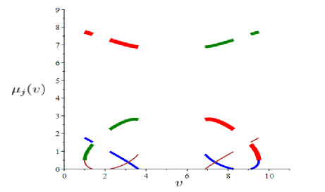
(a)

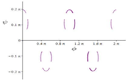
(b)

Figure 1: (a). All the branches of the fibre of possible inverse mass configurations of $\mu_{j}(v)$, for $j=1,2,3,4$ with colors red, green, blue, brown and thicknesses 8, 6, 4, 2, respectively. (b). The fibre is contained in an ellipsoid, leading to the shown distribution of inverse masses in spherical co-ordinates with horizontally the azimuth $\phi$ and vertically the inclination $\psi$. The continuous curves correspond to the branches of the fibre in fig. (a) and the dotted curves correspond to the translates of the branches under the dihedral group $D_{4}$. All these curves on the ellipsoid show that the fibre for the $1{:}2{:}4$ resonance consists of $12$ open curves, compare with [3].

Remark 4.1

From fig. 1a we see that we also have equal masses $\mu_{3}=\mu_{4}$ at two values $v=3.1305722$ and $v=7.3694278$. However, here the cubic normal form does not vanish. The reason is that $\mu_{3}=\mu_{4}$ does not define a symmetry like the $\mathbb{Z}_{2}$–symmetry (13). We therefore defer the discussion of these cases to the general discussion of non-vanishing cubic normal forms in a subsequent paper.

For the $\alpha$–chain ($\beta=0$) at $v=1$ we need two normalising transformations to get the truncated normal form $\mathcal{H}^{4,\lambda}=\mathcal{H}_{2}^{\lambda}+\mathcal{H}_{4}$ with $\lambda=\lambda(\nu)$ in the Hamiltonian (10) and

$$b_{1} = 0$$

$$b_{2} = -\frac{4147}{8640}\>\!\alpha^{2}$$

$$b_{3} = -\frac{17875}{9072}\>\!\alpha^{2}$$

$$b_{4} = -\frac{3\sqrt{286}}{280}\>\!\alpha^{2}$$

$$b_{5} = 0$$ (19)

$$b_{6} = \frac{15053}{7560}\>\!\alpha^{2}$$

$$b_{7} = -\frac{403}{810}\>\!\alpha^{2}$$

$$b_{8} = -\frac{209}{756}\>\!\alpha^{2}$$

in the quartic part (12c). For the general $\beta$–chain ($\alpha=0$) where we do not need to restrict to $v=1$ to have the cubic terms vanish we get the truncated normal form $\mathcal{H}^{4,\lambda}=\mathcal{H}_{2}^{\lambda}+\mathcal{H}_{4}$ with $\lambda=\lambda(\nu)$ in the Hamiltonian (10) and

$$b_{1} = -\frac{3(2v-19)^{2}}{2^{8}(4v-21)^{4}n_{1}^{4}}\left(b_{12}\Gamma^{\frac{3}{2}}\,+\,b_{11}\Gamma^{\frac{1}{2}}\,+\,b_{10}\right)\>\!\beta$$

$$b_{2} = -\frac{3(2v-13)^{2}}{2^{10}(4v-21)^{4}n_{2}^{4}}\left(b_{22}\Gamma^{\frac{3}{2}}\,+\,b_{21}\Gamma^{\frac{1}{2}}\,+\,b_{20}\right)\>\!\beta$$

$$b_{3} = -\frac{3(2v+11)^{2}}{2^{2}(4v-21)^{4}n_{3}^{4}}\left(b_{32}\Gamma^{\frac{3}{2}}\,+\,b_{31}\Gamma^{\frac{1}{2}}\,+\,b_{30}\right)\>\!\beta$$

$$b_{4} = \frac{3\Delta}{\sqrt{2}^{13}(4v-21)^{3}n_{1}^{2}n_{2}n_{3}}\left(b_{42}\Gamma^{\frac{3}{2}}\,+\,b_{41}\Gamma^{\frac{1}{2}}\,+\,b_{40}\right)\>\!\beta$$

$$b_{5} = 0$$ (20)

$$b_{6} = -\frac{3(2v+11)(2v-13)}{2^{5}(4v-21)^{4}n_{2}^{2}n_{3}^{2}}\left(b_{62}\Gamma^{\frac{3}{2}}\,+\,b_{61}\Gamma^{\frac{1}{2}}\,+\,b_{60}\right)\>\!\beta$$

$$b_{7} = -\frac{3(2v+11)(2v-19)}{2^{4}(4v-21)^{4}n_{1}^{2}n_{3}^{2}}\left(b_{72}\Gamma^{\frac{3}{2}}\,+\,b_{71}\Gamma^{\frac{1}{2}}\,+\,b_{70}\right)\>\!\beta$$

$$b_{8} = -\frac{3(2v-13)(2v-19)}{2^{7}(4v-21)^{4}n_{1}^{2}n_{2}^{2}}\left(b_{82}\Gamma^{\frac{3}{2}}\,+\,b_{81}\Gamma^{\frac{1}{2}}\,+\,b_{80}\right)\>\!\beta$$

in the quartic part (12c) where

$$n_{1} = \left(\frac{45(2v-19)[(6v^{2}-57v+107)\sqrt{\Gamma}\,+\,6v^{3}-69v^{2}+229v-256]}{2(-v+\sqrt{\Gamma})(4v-21)}\right)^{\frac{1}{2}}$$

$$n_{2} = \left(-\frac{9(2v-13)[(6v^{2}-39v-52)\sqrt{\Gamma}\,+\,6v^{3}-87v^{2}+388v-256]}{2(-v+\sqrt{\Gamma})(4v-21)}\right)^{\frac{1}{2}}$$

$$n_{3} = \left(\frac{90(2v+11)[(6v^{2}+33v-328)\sqrt{\Gamma}\,+\,6v^{3}-159v^{2}+664v-256]}{(-v+\sqrt{\Gamma})(4v-21)}\right)^{\frac{1}{2}}$$

are defined as in [3] (together with an $n_{4}$ that we do not need here) and

$$b_{12} = 2(4v-21)^{2}(48v^{5}-584v^{4}+3932v^{3}-85074v^{2}+746170v-1877017)$$

$$b_{11} = 8(4v-21)(72v^{8}-1948v^{7}+18782v^{6}-55941v^{5}-331278v^{4}+3089076v^{3}$$

$$\mbox{}\qquad\qquad-6496428v^{2}-10260437v+40373227)$$

$$b_{10} = -(48v^{6}-1512v^{5}+22576v^{4}-196266v^{3}+898339v^{2}-1676472v+368062)$$

$$\mbox{}\!\!\!\!\times\;(28v^{4}-900v^{3}+6419v^{2}-12950v-697)$$

$$b_{22} = 4(4v-21)^{2}(24v^{5}-412v^{4}-422v^{3}+43143v^{2}-298372v+676534)$$

$$b_{21} = 4(4v-21)(144v^{8}-5000v^{7}+66532v^{6}-368922v^{5}-143706v^{4}+12250443v^{3}$$

$$\mbox{}\qquad\qquad-61549224v^{2}+133760048v-122081152)$$

$$b_{20} = -(48v^{6}-1512v^{5}+19504v^{4}-131754v^{3}+436867v^{2}-387240v-682400)$$

$$\mbox{}\!\!\!\!\times\;(28v^{4}-828v^{3}+5999v^{2}-15848v+8048)$$

$$b_{32} = 4(4v-21)^{2}(24v^{5}-892v^{4}+18826v^{3}-29937v^{2}-844720v+3115234)$$

$$b_{31} = 4(4v-21)(144v^{8}-9416v^{7}+245764v^{6}-3135882v^{5}+16325934v^{4}+67107387v^{3}$$

$$\mbox{}\qquad\qquad-1318986636v^{2}+6135153536v-9655555456)$$

$$b_{30} = -(48v^{6}-1512v^{5}+18736v^{4}-115626v^{3}-668141v^{2}+10326288v-28221968)$$

$$\mbox{}\!\!\!\!\times\;(28v^{4}-540v^{3}-721v^{2}+33040v-96832)$$

$$b_{42} = (4v-21)^{2}(48v^{4}-920v^{3}+6676v^{2}-21436v+24965)$$

$$b_{41} = 2(v-1)(4v-21)(144v^{6}-5336v^{5}+76684v^{4}-547544v^{3}+2027809v^{2}$$

$$\mbox{}\qquad\qquad\qquad\qquad-3622625v+2366158)$$

$$b_{40} = -(v-1)(v-4)(v-16)(2v-19)(12v^{2}-126v+277)$$

$$\mbox{}\!\!\!\!\times\;(28v^{3}-512v^{2}+2667v-3713)$$

$$b_{62} = 4(2v-19)(4v-21)^{2}(12v^{4}-212v^{3}+1435v^{2}-6682v+16004)$$

$$b_{61} = 4(2v-19)(4v-21)(72v^{7}-2920v^{6}+43422v^{5}-282828v^{4}+593619v^{3}$$

$$\mbox{}\qquad\qquad\qquad\qquad+1700190v^{2}-8425848v+6257248)$$

$$b_{60} = -(48v^{6}-1512v^{5}+14512v^{4}-26922v^{3}-256469v^{2}+1113924v-830576)$$

$$\mbox{}\!\!\!\!\times\;(28v^{4}-684v^{3}+5231v^{2}-11276v-6304)$$

$$b_{72} = (2v-13)(4v-21)^{2}(48v^{4}-872v^{3}+7924v^{2}-44368v+101273)$$

$$b_{71} = 2(2v-13)(4v-21)(144v^{7}-5720v^{6}+82884v^{5}-525336v^{4}+750405v^{3}$$

$$\mbox{}\qquad\qquad\qquad\qquad+8645652v^{2}-47236533v+73402004)$$

$$b_{70} = -(48v^{6}-1512v^{5}+13456v^{4}-4746v^{3}-542351v^{2}+2893233v-4699028)$$

$$\mbox{}\!\!\!\!\times\;(28v^{4}-720v^{3}+6899v^{2}-29105v+45848)$$

$$b_{82} = (2v+11)(4v-21)^{2}(48v^{4}-968v^{3}+6580v^{2}-16648v+12161)$$

$$b_{81} = 2(2v+11)(4v-21)(144v^{7}-5240v^{6}+80004v^{5}-658896v^{4}+3142173v^{3}$$

$$\mbox{}\qquad\qquad\qquad\qquad-8672760v^{2}+12977859v-8267824)$$

$$b_{80} = -(48v^{6}-1512v^{5}+20752v^{4}-157962v^{3}+687961v^{2}-1579011v+1497904)$$

$$\mbox{}\!\!\!\!\times\;(28v^{4}-864v^{3}+6371v^{2}-17261v+16316)\enspace.$$

Interestingly, at $v=1$ we have $b_{4}=0$. Since $\Delta$ is a factor of $b_{4}$ we also have $b_{4}=0$ at $v=\frac{19}{2}$ where we furthermore have $b_{1}=b_{7}=b_{8}=0$. Adding the $\alpha$– and $\beta$–chain, i.e. working with the full potential (1b) we get at $v=1$ the coefficients

$$b_{1} = \frac{3}{2^{6}}\>\!\beta$$

$$b_{2} = -\frac{11\cdot 13\cdot 29}{2^{6}3^{3}5}\>\!\alpha^{2}\;+\;\frac{7\cdot 41}{2^{8}3}\>\!\beta$$

$$b_{3} = -\frac{5^{3}\cdot 11\cdot 13}{2^{4}3^{4}7}\>\!\alpha^{2}\;+\;\frac{7\cdot 41}{2^{6}3}\>\!\beta$$

$$b_{4} = -\frac{3\sqrt{2\cdot 11\cdot 13}}{2^{3}\cdot 5\cdot 7}\>\!\alpha^{2}$$

$$b_{5} = 0$$ (21)

$$b_{6} = \frac{15053}{2^{3}\cdot 3^{3}\cdot 5\cdot 7}\>\!\alpha^{2}\;+\;\frac{1}{2^{5}3}\>\!\beta$$

$$b_{7} = -\frac{13\cdot 31}{2\cdot 3^{4}\cdot 5}\>\!\alpha^{2}\;+\;\frac{3}{2^{2}}\>\!\beta$$

$$b_{8} = -\frac{11\cdot 19}{2^{2}3^{3}7}\>\!\alpha^{2}\;+\;\frac{3}{2^{3}}\>\!\beta$$

in the quartic part (12c). Note that both $\alpha^{2}$ and $\beta$ are of order $O(\varepsilon^{2})$.

5 Dynamics in one degree of freedom

Here we study the dynamics of a general Hamitonian

$$\mathcal{H}\;\;=\;\;\sigma_{5}\;+\;p_{\eta,\zeta}^{\lambda}\tau_{2}\;+\;q\frac{\tau_{2}^{2}}{2}$$ (22)

on the reduced phase space, a surface given by eq. (14). We defer to the end of this section the discussion of the dependence of the parameters $p_{\eta,\zeta}^{\lambda}$ and $q$ via eq. (15) on the detuning $\lambda=\lambda(\nu)$, the external parameters $\alpha$, $\beta$ and $\mu_{j}$, $j=1,\ldots,4$ of the fpu-chain and the distinguished parameters $\eta$ and $\zeta$. In particular, we assume that the coefficient $b_{4}$ does not vanish in the truncated normal form (15). The orbits of the equations of motion defined by the Hamiltonian (22) coincide with the intersections of the surface (14) with the energy level sets $\{\mathcal{H}=h\}$.

The singular points of the reduced phase space (14) are always equilibria, these occur where $\tau_{2}=2\zeta-\eta\geq 0$. Indeed, for $2\zeta=\eta$ this value is $0$ and the surface of revolution has a cuspoidal singular point, while for $2\zeta>\eta$ this value is positive and the singular point is conical, compare with fig. 2. At $\zeta=\eta$ the reduced phase space (14) shrinks down to a single point, from which the normal–$2$–mode is reconstructed, and also when $\zeta=0$ the reduced phase space is a singular point, corresponding to the normal–$1$–mode $\tau_{1}=2\eta$. The normal–$3$–mode $\tau_{3}={\textstyle\frac{1}{2}}\eta$ is reduced to the cuspoidal singular point $\tau_{2}=0$ at the origin of (14) in case $2\zeta=\eta$. As all three normal modes yield singular points in $1$ dof, the reconstruction of (22) to $3$ dof has three families of periodic orbits in the co-ordinate planes $(x_{j},y_{j})$, i.e. at the normal modes.

Figure 2: The possible forms of the reduced phase space (14) in the intersection with $\{\sigma_{6}=0\}$ given by the curves (24). To get back the surface of revolution (14) one has to rotate the curve(s) about the horizontal axis.

For regular equilibria in $1$ dof the energy level set $\{\mathcal{H}=h\}$ has to be tangent to the reduced phase space (14). The latter is a surface of revolution and the former is a cylinder in the $\sigma_{6}$–direction — on the basis of the intersection (a parabola)

$$\{\mathcal{H}=h\}\;\cap\;\{\sigma_{6}=0\}\;\;:\;\;\sigma_{5}\;=\;h-p_{\eta,\zeta}^{\lambda}\tau_{2}-q\frac{\tau_{2}^{2}}{2}\enspace.$$ (23)

Hence, equilibria $(\tau_{2}^{*},\sigma_{5}^{*},\sigma_{6}^{*})$ necessarily satisfy $\sigma_{6}^{*}=0$. The value $h$ of $\mathcal{H}$ can always be adjusted to let the reduced phase space (14) and the level sets of the Hamiltonian (22) intersect. The two curves that form the intersection of the surface (14) with $\{\sigma_{6}=0\}$ are given by

$$\sigma_{5}\;=\;\pm 4(\eta-2\zeta+\tau_{2})\sqrt{\tau_{2}(\zeta-\tau_{2})}\enspace,\quad\max(0,2\zeta-\eta)\leq\tau_{2}\leq\zeta$$ (24)

and have derivatives

$$\frac{{\rm d}\sigma_{5}}{{\rm d}\tau_{2}}\;\;=\;\;\pm 2\left[2\sqrt{\tau_{2}(\zeta-\tau_{2})}\;+\;\frac{(\eta-2\zeta+\tau_{2})(\zeta-2\tau_{2})}{\sqrt{\tau_{2}(\zeta-\tau_{2})}}\right]\enspace.$$ (25)

We may concentrate on the derivatives of $\sigma_{5}$ with respect to $\tau_{2}$ in eq. (23) and only need to solve the equation

$$\mp\sqrt{\tau_{2}(\zeta-\tau_{2})}(p_{\eta,\zeta}^{\lambda}+q\tau_{2})\;\;=\;\;4\tau_{2}(\zeta-\tau_{2})\;+\;2(\eta-2\zeta+\tau_{2})(\zeta-2\tau_{2})$$ (26)

for $\tau_{2}^{*}$ between $\max(0,2\zeta-\eta)$ and $\zeta$ to obtain the values $(\tau_{2}^{*},\sigma_{5}^{*},0)$ of equilibria, with $\sigma_{5}^{*}$ given by eq. (24). The regular equilibria undergo a centre-saddle bifurcation where the curves given by (23) and (24) not only touch but also have coinciding curvature, resulting in the equation

$$\mp q\sqrt{\tau_{2}^{*}}^{3}\sqrt{\zeta-\tau_{2}^{*}}\;\;=\;\;4\tau_{2}^{*}(\zeta-2\tau_{2}^{*})\;-\;4\tau_{2}^{*}(\eta-2\zeta+\tau_{2}^{*})\;-\;3(\eta-2\zeta+\tau_{2}^{*})(\zeta-2\tau_{2}^{*})$$ (27)

on $\eta$ and $\zeta$. In case the condition (26) holds at the singular point $\tau_{2}^{*}=2\zeta-\eta>0$ this equilibrium undergoes a Hamiltonian flip bifurcation (which reconstructs to a period doubling bifurcation in $2$ dof and to a frequency-halving bifurcation in $3$ dof). Where this happens at $\tau_{2}^{*}=0$ the energy level curve (23) passes horizontally through the singular point reduced from the normal–$3$–mode, resulting in an unstable manifold and thus revealing the normal–$3$–mode to be unstable. Next to $\eta=2\zeta$ (to make $\tau_{2}=0$ a singular point of the reduced phase space) this requires $p_{\eta,\zeta}^{\lambda}=0$, i.e. for the normal form (15) that

$$(b_{3}\,-\,b_{6}\,-\,2b_{8})\zeta\;\;=\;\;2\lambda_{1}\;+\;\lambda_{2}\;-\;\lambda_{3}\enspace.$$

It is helpful to illustrate the dynamics using the contour (24), see fig. 2. Indeed, from these sections one can easily construct the surface of revolution (14), the intersections of which with the parabolic cylinders $\{\mathcal{H}=h\}$ yield the orbits of the reduced dynamics. The parabolic cylinders are determined by the parabolas (23) whence the relative positions of the contour (24) and these parabolas allow to get a full picture of the reduced flow on the surface (14). For $q>0$ the parabolas (23) are ‘upside-down’, with a maximum at

$$\tau_{2}\;\;=\;\;-\frac{p_{\eta,\zeta}^{\lambda}}{q}\enspace.$$

Hence, regular equilibria $(\tau_{2}^{*},\sigma_{5}^{*},0)$ on the lower arc of the contour (24) are elliptic (sometimes the miniml value $h$ of $\mathcal{H}$ is taken at the singular point $\tau_{2}^{*}=2\zeta-\eta$) while on the upper arc we may have both hyperbolic and elliptic equilibria, depending on the centre-saddle and Hamiltonian flip bifurcations (in particular also the maximal value $h$ of $\mathcal{H}$ is sometimes taken at the singular point $\tau_{2}^{*}=2\zeta-\eta$).

The Hamiltonian flip bifurcation occurs where the parabola (23) enters the singular point $\tau_{2}^{*}=2\zeta-\eta>0$ with the same slope as the upper or lower arc of the contour (24). Between these two curves in the $(\zeta,\eta)$–plane the singular equilibrium $\tau_{2}^{*}=2\zeta-\eta>0$ is unstable. Together with the curves (27) of centre-saddle bifurcations these yield the bifurcation diagram shown in fig. 3. For a centre-saddle bifurcation the parabola (23) and the contour (24) have to pass each other non-transversely — the equilibrium where the bifurcation takes place requires that the two curves have to touch each other.

Figure 3: The bifurcation diagram of the dynamics defined by the normal form of the Hamiltonian function (3) with $v=1$ in $1$ dof for $(\alpha,\beta)=(1,0)$ — the $\alpha$–chain — where we put $2\lambda_{1}+\lambda_{2}-\lambda_{3}$ on the horizontal axis, while we normed $\eta=1$ and put $\zeta\in[0,1]$ on the vertical axis. The black lines are centre-saddle bifurcations and the dark grey lines form a circle of Hamiltonian flip bifurcations. The light grey point from which all these lines emerge is where the normal–$3$–mode is momentarily unstable.

To actually compute the bifurcation diagram, the precise dependence of $p_{\eta,\zeta}^{\lambda}$ and $q$ on the external parameters becomes important. For instance, for the normal form (15) we have

$$p_{\eta,\zeta}^{\lambda} \;\;=\;\;\frac{2\lambda_{1}+\lambda_{2}-\lambda_{3}\,+\,4b_{1}(\eta-2\zeta)\,-\,b_{3}\zeta\,+\,b_{6}\zeta\,+\,4b_{7}(\eta-2\zeta)\,-\,2b_{8}(\eta-3\zeta)}{b_{4}}$$ (28)

and

$$q \;\;=\;\;\frac{4b_{1}+b_{2}+b_{3}-2b_{6}+4b_{7}-4b_{8}}{b_{4}}\enspace.$$ (29)

Note that the detuning $\lambda\in\mathbb{R}^{3}$ only enters through the combination $2\lambda_{1}+\lambda_{2}-\lambda_{3}$. In particular, the $\alpha$–chain with $v=1$ has $b_{1},\ldots,b_{8}$ given by (19), whence

$$p_{\eta,\zeta}^{\lambda}\;=\;-\frac{-45360(2\lambda_{1}+\lambda_{2}-\lambda_{3})\,+\,(65192\eta-284997\zeta)\alpha^{2}}{486\sqrt{286}\>\,\alpha^{2}}\quad\mbox{and}\quad q\;=\;\frac{1327579}{1944\sqrt{286}}\enspace.$$

The bifurcation diagram depicted in fig. 3 is for the $\alpha$–chain with $v=1$ for $\alpha=1$. Using (20) one can compute $p_{\eta,\zeta}^{\lambda}$ and $q$ also for the general $\beta$–chain but this leads to bulky formulas.

6 Reconstruction of the dynamics

In this section we reconstruct to higher dof. Reconstructing a degree of freedom amounts to replacing each (regular) point by a circle. The cyclic angle on this circle carries the dynamics that has been reduced. Where the symmetric dynamics approximates a non-symmetric system, the former then is subject to a perturbation analysis to reveal the structure of the latter.

6.1 Reconstruction to $2$ degrees of freedom

While $\mathcal{H}_{2}^{0}$ is always an integral of the normal form, the integral $\mathcal{K}$ of $\mathcal{H}^{4,\lambda}$ is typically made deficient by higher order normal forms (and also by a cubic normal form with non-vanishing $\mathcal{H}_{3}$). Therefore we first reconstruct the dynamics in $2$ dof with the symmetry generated by $\mathcal{H}_{2}^{0}$ still reduced. This consists of attaching an $\mathbb{S}^{1}$ to every regular point of the surface of revolution (14), thereby reconstructing periodic orbits in $2$ dof from regular equilibria in $1$ dof. From the singular point $\tau_{2}=2\zeta-\eta>0$ we also reconstruct a periodic orbit, but of half the period (recall that here the $\mathbb{S}^{1}$–action generated by $\mathcal{K}$ has isotropy $\mathbb{Z}_{2}$). From the cuspoidal point $\tau_{2}=2\zeta-\eta=0$ we reconstruct the normal–$3$–mode, while the normal–$1$ and $2$–modes are reconstructed from the single-point versions of (14) with $\zeta=0$ and $\eta=\zeta$, respectively — where this happens simultaneously we have the $1{:}2{:}4$ resonant equilibrium, which in $2$ dof constitutes $\{\eta=0\}$.

The higher order terms in the normal form yield a slow perturbation of the semi-slow dynamics reconstructed from $1$ dof. In $2$ dof a smooth family of invariant tori is not structurally stable with respect to such integrability-breaking perturbations. However, the periodic orbits constituting the bifurcation diagram of fig. 3 do persist under such perturbations, whence, up to Cantorising families of invariant tori by Diophantine conditions, the integrable dynamics in $1$ dof also governs the perturbed dynamics in $2$ dof.

6.2 Reconstruction to $3$ degrees of freedom

When reconstructing the fast motion along the flow of $X_{\textstyle\!\mbox{\small$H_{2}^{0}$}}$, the normal modes change from being equilibria in $2$ dof to periodic orbits in $3$ dof and only the $1{:}2{:}4$ resonant equilibrium remains an equilibrium. By the same token, the periodic orbits in $2$ dof reconstruct to invariant $2$–tori in $3$ dof and maximal tori reconstruct to maximal tori (of now dimension $3$, with one fast and two semi-slow frequencies).

As any normal form $\mathcal{H}$ of $H$ is by definition equivariant with respect to the flow of $X_{\textstyle\!\mbox{\small$H_{2}^{0}$}}$, the symmetry-breaking terms lead to an exponentially small perturbation. Resonances among the two-timescale-frequencies of maximal tori need a rather high order $k\in\mathbb{Z}^{3}$, but the resonant $3$–tori still break up and lead to (rather small) gaps. Mutatis mutandi for resonant invariant $2$–tori: for elliptic and hyperbolic tori persistence follows from the theory in [2] and for the quasi-periodic centre-saddle bifurcations and the frequency halving bifurcations persistence follows from the theory in [12].

6.3 Reconstruction to $4$ degrees of freedom

Reconstructing the $\mathbb{S}^{1}$-symmetry (2) amounts to rotating the ring of $4$ masses with a velocity governed by $y_{4}={\displaystyle\sum}p_{j}$. This last reconstruction to the full inhomogeneous fpu-chain in $4$ dof is not accompanied by a perturbation analysis as the $\mathbb{S}^{1}$–symmetry (2) is not only a symmetry of the normal form, but a symmetry of the original system as well. Invariant tori reconstruct to invariant tori of one more dimension (which may now have one resonance), in particular the normal modes become invariant $2$–tori and the maximal tori have dimension $4$. In fact, the dynamics of the inhomogeneous fpu-chain with $4$ masses is best understood after reduction to $3$ dof.

7 Conclusions

The reduced $3$ dof inhomogeneous, spatially periodic fpu-chain with two equal masses studied here has an integrable normal form. For the $1{:}2{:}4$ resonance of this chain this holds true in the case of two opposing equal masses, but not for two adjacent equal masses.

The symmetry of the equations of motion induced by our assumption of two opposing equal masses triggers off the existence of the three normal mode periodic solutions. In the original $4$–particles system the normal modes can be reconstructed as a periodic mixture of the particle solutions.

It is expected that breaking the symmetry induced by two equal masses will produce interesting bifurcations. This also gives rise to integrability-breaking phenomena of the normal forms.

Acknowledgements. We thank Roelof Bruggeman and Evelyne Hubert for helpful discussions.

References

- [1] E. van der Aa, First order resonances in three-degrees-of-freedom systems. Cel. Mech. 31 (1983) 163–191
- [2] H.W. Broer, G.B. Huitema and M.B. Sevryuk, Quasi-Periodic Motions in Families of Dynamical Systems: Order amidst Chaos. Lecture Notes Math. 1645, Springer (1996)
- [3] R. Bruggeman and F. Verhulst, The Inhomogeneous Fermi-Pasta-Ulam Chain, a Case Study of the Resonance. Acta Appl. Math. 152 (2017) 111–145
- [4] R. Bruggeman and F. Verhulst, Dynamics of a Chain with Four Particles, Alternating Masses and Nearest-Neighbor Interaction. Chapter 5 in: M. Belhaq (ed.) Recent Trends in Applied Nonlinear Mechanics and Physics. Springer Proc. Phys. 199, Springer (2018) 103–120
- [5] R. Bruggeman and F. Verhulst, Near-Integrability and Recurrence in FPU Chains with Alternating Masses. J. Nonlinear Sci. 29 (2019) 183–206
- [6] H. Christodoulidi, Ch. Efthymiopoulos and T. Bountis, Energy localization on –tori, long-term stability, and the interpretation of Fermi-Pasta-Ulam recurrences. Phys. Rev. E 81(1) 016210 (2010) 1–16
- [7] O. Christov, Non-integrability of first order resonances of Hamiltonian systems in three degrees of freedom, Cel. Mech. & Dyn. Astr. 112 (2012) 147–167
- [8] E. Fermi, Beweis, daß ein mechanisches Normalsystem im Allgemeinen quasi-ergodisch ist. Phys. Z. 24 (1923) 261–265
- [9] E. Fermi, J. Pasta and S. Ulam, Los Alamos Report LA–1940 (1955)
- [10] J. Ford, The Fermi-Pasta-Ulam problem: paradox turns discovery. Phys. Rep. 213 (1992) 271–310
- [11] L. Galgani, A. Giorgilli, A. Martinoli and S. Vanzini, On the problem of energy partition for large systems of the Fermi-Pasta-Ulam type: analytical and numerical estimates. Physica D 59 (1992) 334–348
- [12] H. Hanßmann, Local and Semi-Local Bifurcations in Hamiltonian Dynamical Systems — Results and Examples. Lecture Notes Math. 1893, Springer (2007)
- [13] H. Hanßmann, A. Marchesiello and G. Pucacco, On the detuned resonance. Preprint, Universiteit Utrecht (2019)
- [14] M. Hénon and C. Heiles, The applicability of the third integral of motion: Some numerical experiments. Astronom. J. 69 (1964) 73–79
- [15] B. Rink, Symmetry and resonance in periodic FPU-chains. Commun. Math. Phys. 218 (2001) 665–685
- [16] B. Rink and F. Verhulst, Near-integrability of periodic FPU-chains. Physica A 285 (2000) 467–482
- [17] J.A. Sanders, F. Verhulst and J. Murdock, Averaging Methods in Nonlinear Dynamical Systems, Second Edition. Appl. Math. Sciences 59, Springer (2007)
- [18] R. Schroeders, S. Walcher, Orbit space reduction and localizations. Indag. Math. 27 (2016) 1265–1278
- [19] G.M. Zaslavsky, The physics of chaos in Hamiltonian systems, 2nd extended edition. Imperial College Press (2007)