A local radial basis function method for the Laplace-Beltrami operator
Abstract
We introduce a new local meshfree method for the approximation of the Laplace-Beltrami operator on a smooth surface of co-dimension one embedded in . A key element of this method is that it does not need an explicit expression of the surface, which can be simply defined by a set of scattered nodes. It does not require expressions for the surface normal vectors and for the curvature of the surface neither, which are approximated using formulas derived in the paper. An additional advantage is that it is a local method and, hence, the matrix that approximates the Laplace-Beltrami operator is sparse, which translates into good scalability properties. The convergence, accuracy and other computational characteristics of the method are studied numerically. The performance is shown by solving two reaction-diffusion partial differential equations on surfaces; the Turing model for pattern formation, and the Schaeffer’s model for electrical cardiac tissue behavior.
1 Introduction
Researchers from a diverse range of areas such as medicine, geoscience or computational graphics [1, 3, 6, 14, 18] often urge to find solutions to partial differential equations (PDEs) on surfaces. This is a challenging problem due to the complexity of the differential operators restricted to the geometry of the given surfaces. Among all the methods that seek the solution of this class of PDEs, the most popular are finite element methods, where the equations are solved using surface triangulation [9, 20, 33]. They are in general very efficient but they also have several problems. Specifically, the discretization may not be trivial, and some difficulties may appear when computing geometric primitives such as surface normals and curvatures. Another common approach is to embed the surface PDE within a differential equation posed on the whole , and then restrict the solution to the surface of interest [4, 17, 22]. The main advantage of this method comes from working with cartesian grids. However, the discretization is done in a higher dimensional space and, thus, the computational cost increases. Another disadvantage of these methods is that it is not well understood how the accuracy deteriorates in this procedure.
An alternative approach to estimating the solutions to PDEs on surfaces are global RBF-based methods [15, 16, 21]. They can naturally handle irregular geometries and scattered nodes layouts as no triangularization is needed. Their main advantages are the ease of implementation and the potential spectral accuracy with respect to the number of nodes used to discretize the surface. An additional advantage is that they operate using cartesian coordinates instead of intrinsic coordinates over the surface. However, there are at least two important drawbacks. One is that the computational cost scales as , and thus, it becomes rapidly excessive, making global RBF methods impractical for large problems. The other drawback is that there exists an inverse correlation between the accuracy and the stability of these methods, being the shape parameter that which determines the trade-off between the two. Indeed, they need a somewhat ad-hoc choice of the value of a shape parameter that affects the stability and the ill-conditioning of the resulting linear systems.
To overcome these drawbacks local versions of the global RBF method have also been proposed to solve PDEs defined on a surface [26, 29, 30]. These methods use only a relatively small subset of all the available points to approximate the PDE operator locally, so their cost is largely reduced and the scaling properties improved [13]. As a side effect, the spectral accuracy is sacrificed but much better conditioned linear systems are obtain. In the fewest words possible, local RBF methods inherit many key strengths of global RBF method, with a reduced cost but loosing accuracy.
An interesting consequence of local RBF methods is that they generate finite differences (FD) schemes with certain weights . Hence, they are known as RBF-FD methods. They benefit from some of the key properties of traditional FD approximations, but they are more flexible. While FD are enforced to be exact for polynomials evaluated at the node , RBF-FD are enforced to be exact for RBF interpolants. Thus, weights for FD-like stencils with scattered nodes can be obtained easily.
In [2], we derived a closed-form formula for the (global) RBF-based approximation of the Laplace Beltrami Operator (LBO). It can not only be applied to surfaces whose explicit formula is known, but also to surfaces defined by a set of scattered nodes. The formula only requieres knowledge on the positions of those points, and its accuracy mainly depends on the errors made in the RBF surface reconstruction. If an explicit representation of the surface is given and, therefore, the normal vectors to the surface and its curvature are computed analytically, the convergence is faster than algebraic.
In this paper, we generalize the approach in [2] to local RBF approximations. We carry out a thorough study of the proposed method and analyze its convergence and stability properties when it is applied to reaction diffusion equations over surfaces. We consider the Turing model for pattern formation in nature, and the Schaeffer’s model for electrical cardiac tissue behavior.
The paper is organized as follows. In Section 2, we derive an analytical expression of the LBO applied to a generic RBF, and we characterize the surface defined by a cloud of points in order to approximate the normal vectors and the curvature. In Section 3, we analyze the convergence and stability properties of the proposed method. In Section 4, we apply our approximation to the solution of two different PDEs over surfaces. Section 5 contains our conclusions.
2 Formulation of the problem
Let be a two dimensional surface embedded in , and a set of scattered points distributed on . The objective of this section is to derive a local RBF-FD approximation for the Laplace-Beltrami operator (LBO) applied to a scalar function using the data . We start reviewing the basic concepts of RBF methods necessary to calculate the numerical approximation of a differential operator; see [5, 28, 12] for more details. Then, we describe how to compute the weights for local RBF-FD approximation of the LBO. As in [2], it is also necessary to compute some characteristics of the surface, such as the normal vectors and its curvature, which are also computed using a local RBF methodology. Finally, we describe how to build a differentiation matrix that approximates the action of the LBO in reaction-diffusion type equations on surfaces.
2.1 RBF fundamentals
Radial functions are real valued functions , whose value depends only on the magnitude of its argument, i.e., , where is, usually, the standard euclidean norm. These functions are called Radial Basis Functions (RBF). RBFs can be used to construct interpolants for continuous functions , , sampled at a set of points . Given a set of data ,the interpolant
| (1) |
is constructed as a linear combination of translates of over the points , where the interpolation coefficients are calculated by imposing that the interpolant coincides with the function at each point , so
| (2) |
These requirements lead to the following linear system
| (3) |
where . Notice that the RBF interpolation matrix is dense, symmetric and, under certain conditions, invertible [5].
It is sometimes useful to add a constant to the RBF interpolant (1), so
| (4) |
Adding a constant to the RBF interpolant ensures the exact interpolation of constant functions. It also results in a less oscillatory interpolant, and improves the accuracy of the interpolation [12]. To compute the interpolation coefficients and the constant we impose the conditions (2) with the additional constraint
| (5) |
Then, equation (3) takes the form
| (6) |
where , and are defined in (3), and is a vector with components all equal to 1. Thus, the interpolation problem can be solved calculating the coefficients as
| (7) |
RBFs can also be used to approximate differential operators in a similar way to what is done in the FD method. FD formulas approximate differential operators applied to a function , at a point , by a weighted sum
| (8) |
of the values of that function at a set of neighboring points of . In the standard FD formulation the weights are computed by enforcing (8) to be exact for polynomials of a certain degree evaluated at the set of points , while for RBF, the formula is enforced to be exact for RBF interpolants at those same points [12]. The resulting formulas are called Radial Basis Function-Finite Difference (RBF-FD) formulas.
Thus, given a differential operator and a set of points, the RBF-FD weights are computed by imposing (8) to be exact for the interpolant (4), so
| (9) |
Equation (9) can be written as
| (10) |
where is the weight vector and . Now, using equation (7)
| (11) |
where is the weight vector whose last component is irrelevant in the calculation . From (10), we finally obtain
| (12) |
which is similar to (7) but applied to the differential operator over the RBFs evaluated at the point .
There are several types of RBFs, and the choice of the optimal one for a given problem is still an open question. Among the infinitely differentiable RBFs, those used most often are the Gaussian , the Inverse Quadratic and the Inverse Multiquadric . All these contain a free parameter , called shape parameter, that controls the flatness of the RBF (the smaller the flatter). These three RBFs are examples of positive definite RBFs that guarantees that the interpolation matrix is invertible [10]. It is well known that large values of the shape parameter lead to well-conditioned linear systems, but to an inaccurate approximation of the operator. On the other hand, small values of this shape parameter lead to accurate results but make the condition number of the interpolation matrix large, and hence, the interpolation coefficients may diverge [5].
2.2 RBF-FD for Laplace-Beltrami operator
To obtain an RBF-FD approximation to the LBO using (12), we start by applying the operator to an RBF. The LBO can be defined as the surface divergence of the surface gradient,
| (13) |
Here is the surface operator, which is defined as the orthogonal projection of the usual onto the tangent plane to the surface at each point . Thus,
| (14) |
where is the unit normal vector to the surface.
We start by computing the surface gradient of an RBF . Taking into account that only depends on the distance and applying the chain rule, we obtain
| (15) |
Using the fact that equation (2.2) can be written as
| (16) |
Here, and in all that follows, we write and to simplify the notation.
To complete our calculation of the LBO of an RBF using (13), we take the surface divergence of (16), obtaining
| (17) |
For the first term of this equation we have
| (18) |
where we note that the last term is zero because is the scalar product of two perpendicular vectors. Furthermore,
| (19) |
and
| (20) |
because and
For the second term of equation (2.2), using (16), we have
| (21) |
Noting that is the norm of the projection of over the tangent plane, and applying the Pythagoras Theorem we have Finally, collecting the terms (18)-(21), we obtain
| (22) |
where is the curvature term.
In summary, to compute the value of the LBO applied to an RBF at a certain node , , we consider the stencil centered in and size , which is defined as a subset of consisting of and the nearest neighbor nodes. Without loss of generality, we consider that the center of the stencil is , and , the remaining nodes in the stencil. Then, from (8)
| (23) |
where the weights are obtained from (12) as
| (24) |
Here, the elements of the vector in the right hand side, , are computed using (22).
2.3 Surface characterization
When the normal vectors and the curvature are unknown, it is necessary to compute them before applying (22). In this section, we describe a procedure to approximate the values of these quantities. The procedure uses a level set formalism and RBF interpolation to construct a local approximation to the surface, which is used to compute their approximate values.
We consider a stencil of size centered at the node where we want to compute and . Assume, as before, that is the center of the stencil and , , the other nodes of the stencil. We start by defining a continuously differentiable level-set function , such that its zero level set
| (25) |
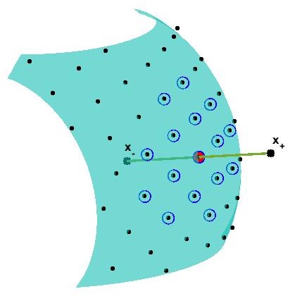
approximates locally the surface in a neighborhood of . To this end, we use an RBF interpolant (4) with the interpolant conditions . We also add two off-surface points and , where has non zero values. The resulting interpolant will then be zero at the nodes of the stencil and non zero elsewhere. The off-surface points are placed at either side of the surface along the direction normal to the surface at (see Figure 1(a)). Although we assume that the normal vectors are not known at this stage, we can approximate them as
where and are two points of the stencil not aligned with .
Thus, we model the local surface implicitly as
| (26) |
where and . The interpolation coefficients and the constant are obtained by enforcing the interpolation conditions (see Figure 1(b))
| (27) |
and the constraint
Once the function is known, the unit normal vector to the surface at a point is simply given by
| (28) |
where the gradient can be computed applying the chain rule
| (29) |
Similarly, the curvature can be obtained from . Note that
| (30) |
where we have used (28) and the relation . Then, using (22) and (16) we obtain
| (31) |
with given by (29). Evaluating (28) and (31) at we obtain approximations to the normal vector and the curvature at each node, respectively.
2.4 RBF-FD solution of reaction-diffusion equations at surfaces
Reaction-diffusion PDEs on surfaces are described by
| (32) |
supplemented with appropriate boundary and initial conditions. Here, represents the variable of interest, the reaction term, the diffusion coefficient, and the LBO that describes diffusion on the surface .
Let be a vector of components containing the values of at the points , . Equation (32) can be spatially discretized as
| (33) |
where is the differentiation matrix containing the RBF-FD weights for the LBO. Equation (33) is a system of coupled ordinary differential equation and, provided it is stable, it can be advanced in time with a suitable time-integration method.
To compute the matrix we start by selecting the size of the stencil at each node, and use (28) and (31) to obtain and , . Then, for each node , we create a vector of components containing the indexes of the nodes in the stencil ( and , , the indexes of the nearest neighbors nodes to ), and use equation (24) to compute the RBF-FD weights , . Each weight is stored as element () of matrix .
A very relevant property that has to be considered is the stability of the time integration method used to solve (32). In general, a minimum requirement for stability is that all eigenvalues of the differentiation matrix lie in the left half-plane of the complex plane. is a sparse matrix, with entries different from zero per row. Unfortunately, the construction of this matrix does not guarantee that all its eigenvalues lie on the left half-plane and, therefore, stability is not ensured. Fortunately, however, we have found that, if the nodes are suitably chosen and if the internodal distance is small enough, then the eigenvalues do in fact lie in the left half-plane. Finding the conditions that could guarantee this property is still an open problem. In this context, the value of the shape parameter and the distribution of the nodes are crucial [16, 30].
3 Numerical tests
In this section, we present numerical experiments whose aim is to test the performance of the proposed procedure to approximate the LBO. These experiments are focused (i) on the convergence of the numerical approximation to the LBO applied to a function at a point, (ii) the quality of the characterization of the surface and (iii) the stability properties of the differentiation matrix resulting from the method described in the previous section. All numerical experiments have been perform using scattered points distributed on the surface of the unit sphere . The used scattered points are uniformly distributed Minimal Energy (ME) nodes, which correspond to the equilibria locations of mutually repelling particles. The exact locations of these ME nodes have been obtained from the repository [24]. In all the experiments we use Gaussians as RBFs.
3.1 Convergence
In the first test, we estimate the error of the numerical approximation to using equation (23). We apply this operator to the function , whose exact is
| (34) |
Note that in the case of the unit sphere, if then and (see [2] for details). The error at location is given by
| (35) |
where are the locations of the nearest neighbors to .
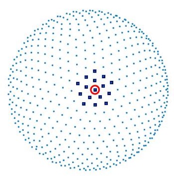
For this experiment we have used ME nodes which are shown in Figure 2(a). The stencil center is (marked with a red circle in the Figure), and the stencil size is . The stencil nodes are shown with thick blue dots.
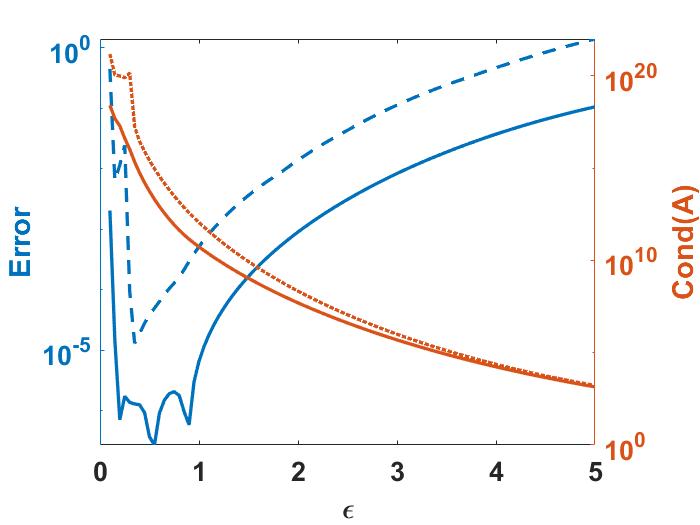
Figure 2(b) shows the resulting error (35) with a continuous blue line, and the condition number of the interpolation matrix with a continuous brown line, as a function of the shape parameter . As expected, when the value of decreases, the condition number increases and the error decreases until we reach a value of where the interpolation matrix becomes ill-conditioned and the error begins to increase sharply.
If instead of considering a single node and its corresponding stencil we repeat the experiment for all the nodes and compute the maximum error and maximum condition number, we obtain the results shown with dashed lines in the Figure. We observe that the behavior is similar to that shown for the case of a single point but the errors and condition numbers are higher. As we can see, there is an optimal value of the shape parameter for which the error is minimum.
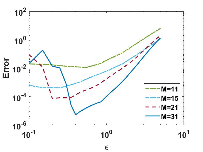
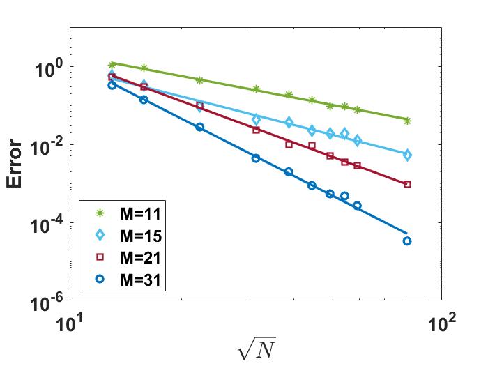
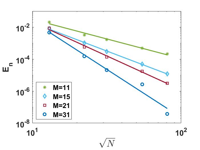
To analyze the order of convergence of the method we have numerically analyzed, for different values of the stencil size, the dependence of the error on the shape parameter and on the internodal distance, which is inversely proportional to . These results are shown in Figures 3(a) and 3(b). We use in Figure 3(a), and in Figure 3(b). Notice that the optimal shape parameter increases with increasing stencil size. Also notice that the convergence rate with is algebraic, while in the global method the convergence is spectral [2]. To confirm this fact we compute the value of the order that best matches the numerical results (Error ). We find for stencils sizes . As expected, the convergence rate increases with the stencil size.
3.2 Surface characterization
In this Section, we analyze the accuracy in the computation of the normal vector (28) and the curvature (31) using the procedure described in Section 2.3. For simplicity, we carry out this analysis for the case of the unit sphere , for which the exact values of the normal vector and curvature are known.
Figure 4 (a) shows the maximum error in the infinity norm of the normal vector, , , as a function of the shape parameter. Figure 4 (b) shows the maximum error in the computation of the curvature, , , as a function of the shape parameter. In both Figures we use ME nodes.
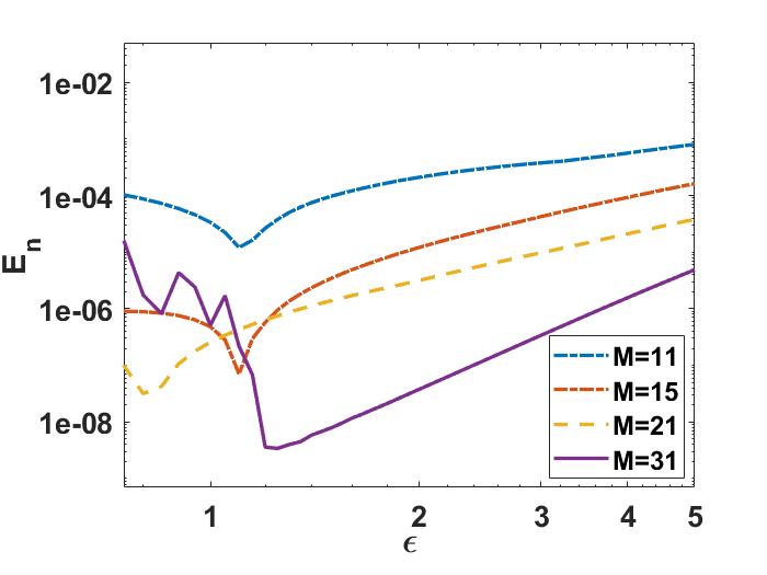
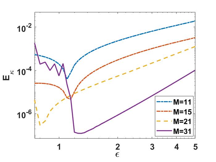
Again, the error decreases with decreasing until the condition number of the interpolation matrix becomes very large and round-off errors deteriorate the accuracy. Also observe that the error decreases with increasing stencil size.
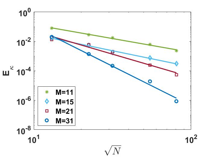
Figures 4 (c) and (d) show the errors in normal vector and curvature ( and , respectively) as a function of . We observe that, similarly to what happened with the error in the approximation to the LBO, see Figure 3(b), convergence is algebraic. We have computed the value of the order that best matches the numerical results. In the case of the error in the approximation to the normal vector, we have obtained for stencil sizes , respectively. Lines with these slopes have been plotted in Figure 4 (c). In the case of the curvature error, we have obtained for the same stencil sizes. Lines with these slopes are also plotted in this figure.
3.3 Stability analysis
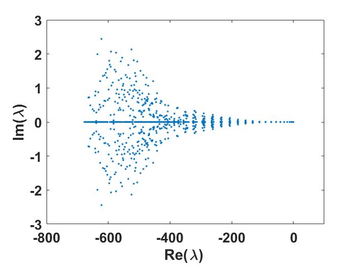
As mentioned in Section 2.4, the eigenvalues of the differentiation matrix determine the stability of the numerical time integration of reaction-diffusion equations over a surface. Here, we consider the differentiation matrix corresponding to the unit sphere for the case of ME nodes, stencil size, and shape parameter. The exact eigenvalues of the Laplace-Beltrami operator are real and non positive; see Chapter 3 of [31]. Their exact values are , with multiplicity
| (36) |
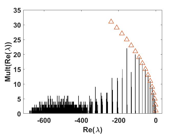
Figure 5 (a) shows the eigenvalues of the matrix. All of them have negative real part, and for small values of they are very close to the exact ones ( for ). This can be better observed in Figure 5 (b) which shows the histogram of the real part of eigenvalues (the imaginary part is approximately zero).Since the height of the histogram represents the number of eigenvalues of a certain value, that height represents the multiplicity of the eigenvalue. The exact multiplicity of the eigenvalues given by (36) are shown with triangles. Notice that, for small values of , the exact multiplicities of the eigenvalues of the Laplace-Beltrami operator are in very good agreement with the multiplicities of the eigenvalues of the differentiation matrix .
4 Numerical results
In this section we apply the method that we propose for the numerical approximation of the LBO in order to compute the solution of two examples of reaction-diffusion problems on surfaces.
4.1 First example:Turing Patterns
As a first example, we consider the reaction-diffusion system proposed by Alan Turing as a prototype model for pattern formation in nature [34]. These patterns arise from a homogeneous and uniform initial state. Turing’s model can generate a variety of spatial patterns which originate from a wide variety of phenomena: morphogenesis in biology [23], ecological invasion [19] or tumor growth [7].
Turing’s equations model the interaction of an activator and an inhibitor . This interaction is described by the following two differential equations:
| (37) | ||||
| (38) |
Depending on the choice of parameters different patterns can arise naturally out of a homogeneous, uniform state. Both variables, and , can lead to instabilities which evolve to different pattern formations, such as stripes or spots.
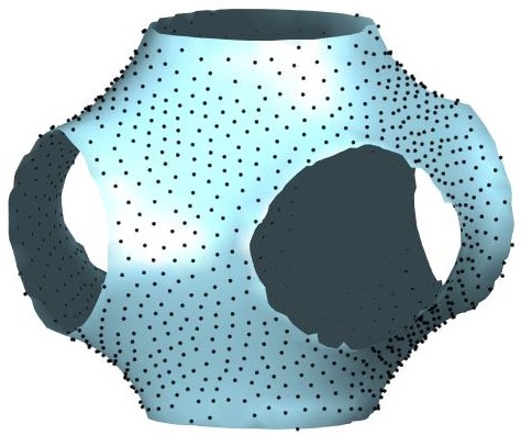
The surface chosen to solve equations (37) and (38) is the Schwarz Primitive Minimal Surface which can be approximated by the implicit equation [27]
| (39) |
We consider periodic boundary conditions in the three coordinate axes, that is, and and the same for the Y- and Z-axes.
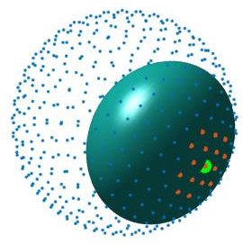
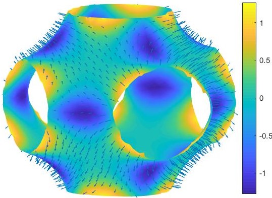
Figure 6 (a) shows the surface (39) and the nodes used for the computation. These nodes have been obtained by projecting radially over Schwarz’s surface a set of ME nodes on the unit sphere obtained from the repository [24]. With this set of nodes, we calculate the normal vectors and the curvature on the surface using equations (28) and (31), respectively. The resulting values are shown in Figure 6 (b). These values have been obtained using a stencil size and a shape parameter . Since the analytic formula of the surface is known (39) we can calculate the exact values of and and, thus, the error. We find that these errors are smaller than 0.1 both for the normal vectors and for the curvature.
The approximate values of and are then used to compute the differentiation matrix of the Laplace-Beltrami operator . In this computation we have used stencils and . We have also checked that the eigenvalues of this matrix do not have positive real part.
For temporal integrations we use function ode45 from MatLab, a standard solver for non-stiff ordinary differential equations. This function implements a Runge-Kutta method with a variable time step for efficient computation.
| pattern | |||||||
|---|---|---|---|---|---|---|---|
| spots | 0.899 | -0.91 | -0.899 | 0.02 | 0.2 | ||
| stripes | 0.899 | -0.91 | -0.899 | 3.5 | 0 |
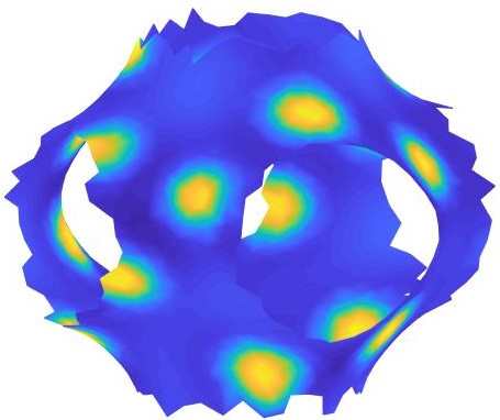
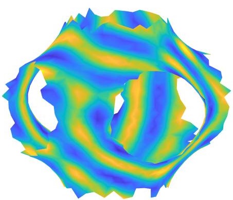
The initial condition in both cases is a perturbation of the activator . The interaction between the activator and the inhibitor results in a transient state that, for long times, evolves to a stationary state with different characteristic patterns which depend on the values of the parameters. Figures 6 (c) and (d) show the stationary states corresponding to the two sets of parameters shown in Table 1, which have been taken from [30]. These two stationary states correspond to two classic patterns of Turing’s model: the spots and the stripes pattern, respectively. These stationary states are in agreement with those obtained previously for the same parameters [30].
4.2 Second example: Schaeffer’s model
In the second numerical experiment we solve the bioelectric cardiac source model proposed by Mitchell and Schaeffer [25]. This is a simple model which is capable of reproducing the main electrophysiological properties of cardiac tissue, such as restitution properties or spatial variations of the action potential duration. The model consists of two differential equations
| (40) |
and
| (41) |
where and are the transmembrane voltage and the inactivation gate variable, respectively. In (40), the terms and represent the inward and outward currents of the cells of the membrane
| (42) |
and represents the initial stimulus. The diffusive term models the transmembrane current flowing through the cardiac membrane. The six parameters , and govern the behavior of the membrane and, depending on their values, they can not only model healthy tissue, but also tissue with some kind of pathology. We refer the interested reader to [25, 1] for more details about this model.
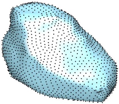
We have applied our proposed procedure to the solution of equations (40)-(42) with the parameters shown in Table 2. These equations are solved on the epicardium, which is the outermost surface membrane of the heart and which is shown in Figure 7(a). We also show the points used for the numerical solution of the problem. These points have been obtained from a computerized tomography (CT) of a real patient [8]. Therefore, it is a realistic model in which we do not have information neither on the normal vectors nor on the curvature of the surface. We consider
as initial conditions, and we apply a current stimulus
| (43) |
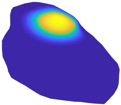
shown in Figure 7(b). Here, denotes the Heavisade function, the time when the stimulus ends, the position where the stimulus is applied, and its spatial width.
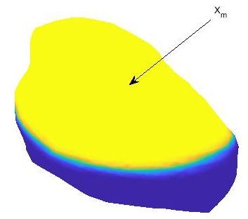
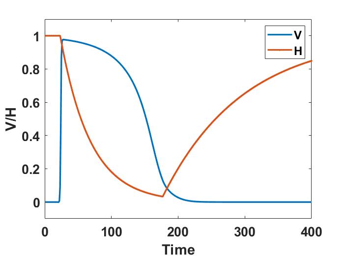
We use the same method that in the previous example for temporal integration. The solution shows the propagation of the electric excitation along the membrane. For instance, Figure 7 (c) shows the transmembrane current 50 ms after the stimulus ends. The tissue goes from a resting to an excited state. Finally, the membrane returns to the resting state awaiting for the next stimulus. This behavior can be observed in Figure 7 (d), where we show the evolution with time of the transmembrane voltage and the gate variable at the point in Figure 7 (c). As we can see, the cardiac tissue experiences the different stages of a heartbeat corresponding to those shown in [25].
5 Conclusions
In this article we have introduced a new RBF-FD based method to calculate the solution of reaction-diffusion equations over surfaces. The diffusive part of this kind of equations is usually modeled by the LBO, for which we calculate a numerical approximation, , using an RBF-FD approach. This approach is based on an explicit formula for the LBO applied to an RBF, which is exact; see (22). This formula involves the normal vectors and the curvature to the surface. These are known if an explicit expression for the surface is available. If the surface is defined by a set of scattered nodes which is the usual output of, for example 3D scanning processes, we propose a level set formalism and an RBF interpolation to construct a local approximation to the surface, from which we estimate these quantities.
We have study numerically the convergence and stability properties of our approach, and we have shown the performance of the proposed methodology solving the Turing model for natural pattern formation over a Schwarz Primitive Minimal Surface, and the Schaeffer’s model for electrical cardiac tissue behavior.
6 Acknowledgments
This work has been supported by Spanish MICINN Grant FIS2016-77892-R.
References
- [1] D. Alvarez, F. Alonso-Atienza, J.L. Rojo-Alvarez, A. Garcia-Alberola, M. Moscoso, Shape reconstruction of cardiac ischemia from non-contact intracardiac recordings: a model study, Math. Comput. Model. 55 (2012) 1770–1781 .
- [2] D. Alvarez, P. Gonzalez-Rodriguez, and M. Moscoso, A Closed-Form Formula for the RBF-Based Approximation of the Laplace-Beltrami Operator, J. Sci. Comput. (2018) 77: 1115.
- [3] R. Barreira, C.M. Elliott, and A. Madzvamuse, The surface finite element method for pattern formation on evolving biological surfaces, J. of Math.Biology. 63 (2011) 1095–1119.
- [4] M. Bertalmio, L.-T. Cheng, S. Osher, and G. Sapiro, Variational problems and partial differential equations on implicit surfaces, J. Comput. Phys. 174 (2001) 759–780.
- [5] M.D. Buhmann, Radial Basis Functions, Cambridge University Press (2003)
- [6] J. C. Carr, R. K. Beatson, J. B. Cherrie, T. J. Mitchell, W. R. Fright, B. C. McCallum, and T. R. Evans. 2001. Reconstruction and representation of 3D objects with radial basis functions. In Proceedings of the 28th annual conference on Computer graphics and interactive techniques (SIGGRAPH ’01). ACM, New York, NY, USA, 67-76. DOI: https://doi.org/10.1145/383259.383266
- [7] M.A. Chaplain,M. Ganesh and I.G. Graham, Spatio-temporal pattern formation on spherical surfaces: numerical simulation and application to solid tumour growth, J. Math. Biol. (2001) 42(5):387-423.
- [8] C. E. Chavez,N. Zemzemi, Y. Coudi�re, F. Alonso-Atienza and D.Alvarez, Inverse Problem of Electrocardiography: estimating the location of cardiac isquemia in a 3D geometry. Functional Imaging and modelling of the heart (FIMH2015), Maastricht, Netherlands. 9126, Springer International Publishing, 2015,
- [9] G. Dziuk and C. Elliott, Surface finite elements for parabolic equations, J. Comp. Math. 25 (2007) 385–407.
- [10] G.E. Fasshauer, Meshfree Approximation Methods with Matlab, World Scientific Publishers, 2007.
- [11] M. Floater and K. Hormann, Surface parameterization: a tutorial and survey, Advances in Multiresolution for Geometric Modelling, Springer, 2005.
- [12] B. Fonberg and N. Flyer, A primer on radial basis functions with applications to geosciences, CBMS-NSF Regional Conference Series in Applied Mathematics (2015).
- [13] B. Fornberg and E. Lehto, Stabilization of RBF-generated finite difference methods for convective PDEs, Journal of Computational Physics 230 (2011) 2270-2285.
- [14] N. Flyer and B. Fornberg, Radial basis functions: Developments and applications to planetary scale flows, Computers and Fluids, 26 (2011) 23–32.
- [15] N. Flyer and G. B. Wright, A radial basis function method for the shallow water equations on a sphere, Proc. Roy. Soc. A 465 (2009) 1949–1976.
- [16] E. J. Fuselier and G. B. Wright, A high order kernel method for diffusion and reaction-diffusion equations on surfaces, Journal of Scientific Computing (2013) 1-31.
- [17] J. B. Greer, An improvement of a recent Eulerian method for solving PDEs on general geometries, J. Sci. Comput. 29 (2006) 321–352.
- [18] X. Gu, Y. Wang, T. Chan, P. Thompson, and S. Yau, Genus zero surface conformal mapping and its application to brain surface mapping, Medical Imaging, IEEE Transactions on, 23 (2004), pp. 949–958.
- [19] E. E. Holmes, M. A. Lewis, J. E. Banks and R. R. Veit, Partial Differential Equations in Ecology: Spatial Interactions and Population Dynamics, Ecology (1994) 75(1), 17-29.
- [20] M. Holst, Adaptive numerical treatment of elliptic systems on manifolds, Advances in Computational Mathematics 2001 139–191.
- [21] E. Lehto, V. Shankar, and G. B. Wright, A Radial Basis Function (RBF) Compact Finite Difference (FD) Scheme for Reaction-Diffusion Equations on Surfaces, SIAM J. Sci. Comput. (2017) 39 (5) A2129-A2151.
- [22] C. B. Macdonald and S. J. Ruuth, The Implicit Closest Point Method for the Numerical Solution of Partial Differential Equations on Surfaces, SIAM J. Sci. Comput. 31 (2009) 4330–4350.
- [23] P. K. Maini, T. E. Woolley, , R. E. Baker, E. A. Gaffney, and S. S. Lee, Turing’s model for biological pattern formation and the robustness problem, Interface focus (2012) 2(4), 487-496.
- [24] https://web.maths.unsw.edu.au/ rsw/Sphere/Energy/index.html
- [25] C.C.Mitchell, D. G. Shaeffer, A Two-Current Model for the Dynamics of Cardiac Membrane, B. Math. Biol. 65 (2003), 767-793.
- [26] C. Piret , The orthogonal gradients method: A radial basis functions method for solving partial differential equations on arbitrary surfaces, J. Comput. Phys. (2012) 231, 4662-4675
- [27] http://www.msri.org/publications/sgp/jim/geom/level/library/triper/index.html
- [28] S.A. Sarra and E.J. Kansa Multiquadric radial basis function approximation methods for the numerical solution of partial differential equations, Adv. Comput. Mech., 2 (2009)
- [29] V. Shankar, G. B. Wright, A. L. Fogelson and R. M. Kirby, A study of different modeling choices for simulating platelets within the immersed boundary method, Appl. Numer. Math. (2013) 63, 58?77
- [30] V. Shankar, G. B. Wright, R. M. Kirby and A. L. Fogelson A radial basis function (RBF)- finite difference (FD) method for Diffusion and reaction Diffusion equations on surfaces, J. Sci. Comput. (2015) 53: 745-768.
- [31] M.A. Shubin (2001) Asymptotic Behaviour of the Spectral Function. In: Pseudodifferential Operators and Spectral Theory. Springer, Berlin, Heidelberg
- [32] J. Stam, Flows on surfaces of arbitrary topology, ACM Trans. Graph. 22 (2003) 724–731.
- [33] G. Turk. Generating textures on arbitrary surfaces using reaction-diffusion, volume 25 ACM 1991.
- [34] M. A. Turing, The chemical basis of morhogenesis,Phil. Trans. R. Soc. (1952) B237,37-72.