Adversarial Attacks to Scale-Free Networks: Testing the Robustness of Physical Criteria

Abstract

Adversarial attacks have been alerting the artificial intelligence community recently, since many machine learning algorithms were found vulnerable to malicious attacks. This paper studies adversarial attacks to scale-free networks to test their robustness in terms of statistical measures. In addition to the well-known random link rewiring (RLR) attack, two heuristic attacks are formulated and simulated: degree-addition-based link rewiring (DALR) and degree-interval-based link rewiring (DILR). These three strategies are applied to attack a number of strong scale-free networks of various sizes generated from the Barabási-Albert model. It is found that both DALR and DILR are more effective than RLR, in the sense that rewiring a smaller number of links can succeed in the same attack. However, DILR is as concealed as RLR in the sense that they both are constructed by introducing a relatively small number of changes on several typical structural properties such as average shortest path-length, average clustering coefficient, and average diagonal distance. The results of this paper suggest that to classify a network to be scale-free has to be very careful from the viewpoint of adversarial attack effects.

I Introduction

Scale-free networks are ubiquitous in nature and society, from email networks Ebel, Mielsch, and Bornholdt (2002) to cell networks Albert (2005), from World-Wide Web Albert, Jeong, and Barabási (1999) to social networks Xuan et al. (2019), and beyond. In a scale-free network, few nodes have large numbers of connected links, exhibiting remarkable heterogeneity in node degrees. This special feature makes them be highly robust against random attacks but extremely vulnerable to targeted attacks, which is known as the Achilles Heel effect.

Since the influential report on scale-free networks Barabási and Albert (1999), referred to as the Barabási-Albert (BA) network model, there have been a lot of studies Barabási, Albert, and Jeong (1999); Molontay and Nagy (2020). Generally, a network is considered to be scale free if its degree distribution follows a power-law form, i.e., $p(k)\sim k^{-\alpha}$, where $k$ is the node degree and $\alpha$ is the power-law exponent. In some cases, the definition is stricter. For example, it may require that the power-law exponent satisfies $\alpha\in(2,3)$ or its generation mechanism has a preferential attachment operation Dorogovtsev and Mendes (2002). In some other cases, the definition is broader. For example, it may only require the upper tail of the degree distribution curve to satisfy the power-law form Willinger, Alderson, and Doyle (2009), or its log-log curve is nearly straight. The discussions on the definition of a scale-free network has attracted considerable attention since the early 2018, when Broido and Clauset Broido and Clauset (2019) proposed a classification method to estimate the strength of the scale-free attribute of a network. They tested nearly 1,000 real networks and concluded that scale-free networks are rare. Yet, Barabási Barabási (2018) believes that there are some deficiencies in their preprocessing of the real network data: when transforming a network to several simple degree sequences, the weights for various degree sequences should be different. Voitalov et al. Voitalov et al. (2018) pointed out that if the fitted model is a pure power-law model, there is no question that scale-free networks are rare, but in real life, due to the existence of noise, sampling or other processing factors, it is not possible to obtain a pure power-law distribution. Coincidentally, in machine learning, there are many recent studies showing that it is quite possible to output an erroneous result when some slight disturbance such as noise is applied to the input data, which is called adversarial attack Szegedy et al. (2013). Consequently, a great deal of interest is aroused to revisit the notion of adversarial attacks.

Noise plays an important role in many aspects of data analysis. Since deep learning is widely used in computer vision Xuan et al. (2017a, 2018), there are a number of studies on algorithm robustness Papernot et al. (2016); Su, Vargas, and Sakurai (2019); Moosavi-Dezfooli, Fawzi, and Frossard (2016); Xie et al. (2017). It was found that changing a few pixels in an image could make the classification result totally wrong or different. The reason is that the feature vector of the image will change when a pixel is modified, which can fool many deep learning algorithms. For example, Su et al. Su, Vargas, and Sakurai (2019) changed only one pixel in an image, they were able to destroy many intrinsic properties of the image and fool a deep neural network. Besides, there are many other ways to add such disturbances to an image, e.g., FGSM Goodfellow, Shlens, and Szegedy (2014), ILCM Kurakin, Goodfellow, and Bengio (2016), DEEPFOOL Moosavi-Dezfooli, Fawzi, and Frossard (2016), and so on. Most of these methods can only generate a specific disturbance for a specific image, instead Moosavi-Dezfooli et al. Moosavi-Dezfooli et al. (2017) created general perturbations for a bunch of images, making the situations even worse, since such disturbances are not easily identifiable by human.

Besides computer vision, in the area of network science it was also found that simple purposeful modifications to an original network, i.e. by rewiring links, adding/deleting nodes or changing nodes’ attributes, can significantly change the network properties and thus greatly disturb the graph algorithms Dai et al. (2018). Recently, a number of strategies were proposed to attack link prediction Fu et al. (2018); Chen et al. (2019a), node classification Wang et al. (2018), and community detection Chen et al. (2019b). For instance, Yu et al. Yu et al. (2019) proposed heuristic and evolutionary algorithms to protect targeted links from link-prediction-based attacks. Zügner et al.  Zügner, Akbarnejad, and Günnemann (2018) considered attacking node classification, and introduced NETTACK based on a graph convolutional network (GCN) to generate adversarial attack iteratively. Chen et al. Chen et al. (2019b) used genetic algorithm (GA)-based $Q$-attack to destroy the community structure of a network, where the modularity $Q$ is used to design the fitness function.

On the other hand, $p$-value is dominant in statistical analysis, which however has been questioned before Evans, Mills, and Dawson (1988). Today, the $p$-value measure has been re-examined and advanced to a new climax Amrhein, Greenland, and McShane (2019). More than 800 reports pointed out that the sample size has a great impact on the $p$-value. By adding or subtracting some data, which can be considered as noise, one will get a different result compared with the original one. This explains why most experimental results obtained by using $p$-values are difficult to reproduce.

The reality is, unfortunately, what you see from the data may not mean what they really are. In other words, the algorithms and models developed based on real data could be vulnerable to tiny noise and purposefully designed noise-like perturbations. Therefore, the robustness of machine learning algorithms attracts more and more attention from the Artificial Intelligence (AI) community. The robustness of many physical criteria, especially those based on data, have to be examined to ensure that they are reliable.

Motivated by the above discussions, in this paper, a new type of adversarial attack is introduced to the robustness of physical criteria on scale-free networks. Specifically, three attack strategies are used to evaluate the robustness of the classification method proposed for scale-free networks Broido and Clauset (2019). To be convincing, the Barabási-Albert (BA) model is used to generate 100 strong scale-free networks of different sizes for testing the attacks in experiments, by rewiring some links of these networks until the Broido-Clauset (BC) Broido and Clauset (2019) classification goes wrong. The results show that the BC classification can be easily fooled by rewiring only a small fraction of links.

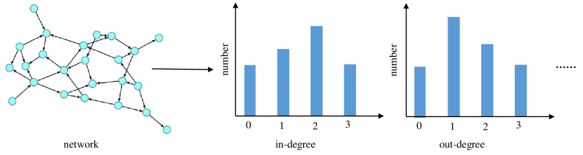
Figure 1: Preprocessing of a real-world network under the BC classification framework. Taking a directed network as an example, the directed attribute is removed and both in-degree and out-degree sequences are obtained.

The main contributions of this paper are summarized as follows.

• A new adversarial attack is introduced onto the physical criteria of scale-free networks to evaluate the robustness of the scale-free measure.

• Two heuristic attack strategies, namely degree-addition-based link rewiring (DALR) and degree-interval-based link rewiring (DILR), are introduced. Several structural metrics are proposed to measure the effectiveness and concealment of the attack strategies.

• It is found that both DALR and DILR are more effective than random link rewiring (RLR), in terms of rewiring fewer links to successfully attack strong scale-free networks, so that the networks become other types. It is also found that DILR is as concealed as RLR in that they both are constructed by introducing a relatively small number of changes on several typical structural properties such as average shortest path-length, average clustering coefficient, and average diagonal distance. Therefore, the results of this paper suggest that to classify a network to be scale-free has to be very careful from the viewpoint of adversarial attack effects.

The rest of the paper is organized as follows. The BC classification of scale-free networks is introduced in Sec. II. Three adversarial attack strategies are proposed in Sec. III. Some metrics for attack effectiveness and concealment are discussed with experimental results reported in Sec. IV. Conclusions are drawn in Sec. V.

II Classification of scale-free networks

Here, the classification of scale-free networks proposed by Broido and Clauset Broido and Clauset (2019) is reviewed, which is referred to as the BC classification below.

• First, preprocessing the real-world network data. Common analysis typically relies on the scale-free hypothesis to determine whether a network is scale-free or not. This hypothesis states that a network is scale-free if its degree distribution follows a power-law form, where only the information of node degree is taken into account. While real-world networks carry many irrelevant attributes such as link weights, connection directions, etc., which make it inconvenient to estimate the strength of the scale-free attribute. Thus, the BC classification suggests to first convert the original network to a set of simple graphs, where one can apply the scale-free hypothesis to each graph. In this way, one can obtain several degree sequences. For example, from a directed network, one can get an in-degree sequence and an out-degree sequence (see Fig. 1). To that end, one can put all the degree sequences in a set, $S$.

• Second, estimating the strength of scale-free attribute. Several indicators are used in BC classification to estimate the strength of scale-free attribute for a given network, which are listed in TABLE 1, where $R$ is one newly proposed here to evaluate the best fit model.

  Table 1: Indicators for the scale-free attribute in BC classification.

  Indicators	Description
  $\alpha$	Power-law exponent obtained by fitting a power-law degree distribution model.
  $n_{tail}$	Number of tail nodes used for fitting.
  $p$	$p\geq 0.1$: Accept the scale-free hypothesis.
  	$p<0.1$: Reject the scale-free hypothesis.
  $R$	$R>0$: The power-law model is much in favor.
  	$R=0$: The data do not permit a distinction between (power-law or alternative) models.
  	$R<0$: The alternative model (such as the exponential model) is much in favor.

• Third, classifying the networks. According to the above two steps, one can determine the strength of the scale-free attribute of a network, based on which, the real networks in examination were divided into six categories: strongest, strong, weak, weakest, super-weak, and non-scale-free, as shown in Fig. 2. It can be seen that the strongest, strong, weak, and weakest classes are nested, indicating that the strength of the scale-free attribute becomes weaker gradually. The super-weak class indicates that the networks are extremely weak in scale-free attribute, which only requires that the optimal distribution is in a power-law form. Networks that do not fall into the above five categories are considered as non-scale-free networks.

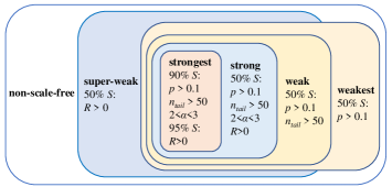
Figure 2: The real-world networks in examination are classified into six categories Broido and Clauset (2019): strongest, strong, weak, weakest, super-weak, and non-scale-free.

Broido and Clauset Broido and Clauset (2019) analyzed nearly 1,000 networks in different domains, and they found that only a small number of them can be considered as strong scale-free networks. Even the simplex networks generated by the BA model do not entirely belong to the strong category. Thus, they concluded that scale-free networks are rare. This classification method has attracted much attention in the network science community, and triggered wide discussions recently Barabási (2018); Gerlach and Altmann (2019); Voitalov et al. (2018).

III Method

In a computer vision simulation, as an adversarial attack example, tiny perturbations are added into a panda picture. It is very difficult for human to find differences between the attacked picture and the original one. This surprisingly can make the classification algorithm misjudge it to be a gibbon picture with a probability of 99.3% Goodfellow, Shlens, and Szegedy (2014).

In this paper, the idea of adversarial attack is applied to fool the BC classification introduced in the previous section. Specifically, by rewiring a few links in the network to alter the values of the indicators, namely making the indicators exceed the limit of the original category, the attack can make the BC classification results go wrong. According to the BC classification algorithm, the difference between the strong category and the weak category is determined by the power-law exponent $\alpha$ and the indicator $R$ in TABLE 1, and the difference between the weak and weakest categories is determined by $n_{tail}$, the number of fitting nodes. It is emphasized that the power-law exponent $\alpha$ plays an more important role than the indicator $R$ on determining the strong category Broido and Clauset (2019). Therefore, in this paper, the adversarial attack strategy is designed based on the measures of both power-law exponent $\alpha$ and number of fitting nodes $n_{tail}$.

A network is represented by a graph $G=(V,E)$, where $V$ and $E$ represent the sets of nodes and links in the network, respectively. Let $\Omega$ represent the set of links in the fully-connected network with the same set of nodes $V$. Note that $E$ is a part of set $\Omega$. Define $N=\Omega-E$ as the set of links in the complementary network of $G$, namely those in the fully-connected network but are not in network $G$.

III.1 Random Link Rewiring

In the random link rewiring (RLR) scheme, one first randomly selects a link $l_{delete}\in E$ to delete and a link $l_{add}\in N$ to add at each step time, so as to balance the number of links in the network. After an attack, the set $E$ and $N$ become $E^{\prime}$ and $N^{\prime}$, respectively:

$$E^{\prime}=E-l_{delete}+l_{add},$$ (1)

$$N^{\prime}=N+l_{delete}-l_{add}.$$ (2)

Thus, one gets a new adversarial network $G^{\prime}=(V,E^{\prime})$.

III.2 Degree Based Link Rewiring

One of the prominent properties of scale-free networks is that there exist a few nodes with extremely large degrees, called hubs. These hubs are key to the robustness of the networks—they make the scale-free networks be highly tolerant to random attacks while extremely vulnerable to targeted attacks Albert, Jeong, and Barabási (2000), measured by the connectivity or the average shortest path-length of the network. Moreover, they play an important role in some dynamical processes taking place on the networks, like epidemic spreading Pastor-Satorras, Vespignani et al. (2003); Ruan, Tang, and Liu (2012), information cascading Wolfson et al. (2009) and synchronization Wang and Chen (2002); Xuan et al. (2017b).

Degree-Addition-based Link Rewiring (DALR).

Roughly divide the links in a scale-free network into three categories: hub-hub links (links connecting two hubs), hub-normal links (links connecting one hub and one normal node), and normal-normal links (links connecting two normal nodes). Then, DALR is designed based on the following two operators.

• Deleting a hub-hub link. Since the number of hub-hub links in a scale-free network are generally quite small, this condition can be relaxed as follows: first, design an indicator $d_{(i+j)}$ to measure the degree of node pairs:

  $$d_{(i+j)}=d_{i}+d_{j},$$ (3)

  where $d_{i}$ and $d_{j}$ represent the degrees of nodes $v_{i}$ and $v_{j}$, respectively. Then, sort the links according to their values of $d_{(i+j)}$, from large to small. The link with the highest ranking will be chosen to remove.

• Adding a normal-normal link. In order to weaken the scale-free attribute without changing the network density, add a normal-normal link, since this operation can weaken the heterogeneity of the network. Specifically, the nodes are sorted according to their degree from small to large, and the link between the pair of unconnected nodes with the smallest sum of degrees is chosen to connect together.

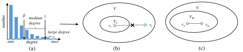
Figure 3: Illustration of DILR attack strategy. (a) Determine the set of large-degree nodes, $V_{L}$, and the set of medium-degree nodes, $V_{M}$, according to the degree sequence. (b) Delete the link between two connected hub nodes (note that, here, node $v_{j}$ has the largest degree among all the neighbors of $v_{i}$, so it could be either in or not in $V_{L}$). (c) Add a link between two unconnected nodes of medium degrees.

Degree-Interval-based Link Rewiring (DILR).

The main indicators of strong and weak categories are the power-law index $\alpha$ and the number of fitting nodes, $n_{tail}$, which are determined by the fitting process. Divide the node distribution into two parts according to the $p$ value: the tail of the distribution used for fitting and the others for another purpose. As is well known, the power-law index $\alpha$ is determined by the (average) slope of the curve; therefore, if the tail is steeper with smaller $n_{tail}$, it will be out of the strong and weak categories much easily.

Based on the above observations, one can roughly divide the nodes into three sets: nodes with large degrees (within $\gamma$=20%), nodes with medium degrees (between $\gamma$ and $\beta$, with $\beta$ varying from 35% to 70%), and nodes with small degrees (the remaining ones), as shown in Fig. 3. Denote $V_{L}$ and $V_{M}$ the nodes of large degrees and medium degrees, respectively. Then, the following DILR attack strategy is designed.

• Deleting a link between two connected hub nodes. First, select a node $v_{i}\in{V_{L}}$, and then choose a $v_{j}\in{N_{i}}$, where $N_{i}$ is the neighboring set of $v_{i}$, such that $v_{j}$ has the largest degree among all neighbors of $v_{i}$. Then, delete the link between $v_{i}$ and $v_{j}$.

• Adding a link between two unconnected nodes of medium degrees. Randomly select two unconnected nodes from $V_{M}$, and add a link between them.

IV Experimental Results

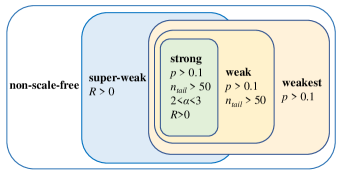
Figure 4: Classification of simplex networks generated by the BA model, in terms of scale-free attribute. Here, strongest and strong categories are merged into one, the strong category, and the other four categories keep the same, as suggested by Broido and Clauset Broido and Clauset (2019).

IV.1 Datasets

There are many models for generating scale-free networks: the BA model Barabási and Albert (1999), fitness model Bianconi and Barabási (2001), and local-world evolving network models Li and Chen (2003); Xuan, Li, and Wu (2006, 2007); Sen and Dai (2009), etc. In this paper, the most well-known BA model is adopted to generate simplex networks. Since all the generated networks are simplex, there will not be the strongest category. In other words, only the following five categories are considered here: strong, weak, weakest, super-weak, and non-scale-free, where the former three are nested, as shown in Fig. 4. In order to test the robustness of the BC classification method, the simulation is to attack the BA network of different sizes: $n=500,\,1000,\,2000$, respectively, where $n$ is the number of nodes. For simplicity, the number of links, $m$, is set to be $2n$.

In the simulation, 500 networks for each size were generated, and then classified. TABLE 2 shows the classification results, where it can be seen that most (but not all) of the networks generated by the BA model indeed fall into the strong category regardless of the sizes of the networks. However, there are still some networks that cannot be considered as scale-free networks by the BC classification, specifically more than 10% of them are considered as super-weak and very few of them are considered as weak. As the network size increases, more networks will be classified into the non-scale-free category.

IV.2 Performance Metrics

IV.2.1 Metric for effectiveness

When attacking a model or scheme, one always hopes that the attack could successfully fool the object with a lowest cost, e.g., changing the least number of pixels to fool a computer vision model, or rewiring the least number of links to fool a link prediction or a node classification algorithm. Here, to measure the effectiveness of different adversarial attack strategies, the smallest fraction of rewired links needed to successfully fool the BC classification method Broido and Clauset (2019) is considered, by changing the strong category of scale-free networks to another type. The metric is defined by

$$\Delta{M}=\frac{m_{R}}{m},$$ (4)

where $m_{R}$ is the smallest number of rewired links to realize a successful attack and $m$ is the total number of links in the whole network. If a (strong) scale-free network is still in the strong category after a large perturbation introduced by the attack, i.e., a large fraction of links are rewired, then it is deemed that the classification algorithm is robust or the attack is less effective.

Table 2: Classification results of the BA network of different sizes. Most (more than 70%) but not all of these BA networks fall into the strong category.

n	strong	weak	weakest	super-weak	non-scale-free
500	89.30%	0.30%	0%	10.30%	0%
1000	78%	0%	0%	20.60%	1.40%
2000	73.60%	0.20%	0%	14.60%	11.60%

IV.2.2 Metrics for concealment

Generally, rewiring a network not only may change the scale-free attribute (the objective here), but also may change other structural properties of the network. In this sense, defenders may utilize certain structural properties to discover the adversarial attack.

To quantify the concealment of various adversarial attacks, the following three metrics are proposed for measuring the structural changes introduced by an attack.

• Relative change of average distance ($\Delta{L}$). The average distance, or shortest path-length, is defined as

  $$L=\frac{2}{n(n-1)}\sum_{i>=j}d_{ij},$$ (5)

  where $n$ is the number of nodes and $d_{ij}$ is the shortest path length between nodes $v_{i}$ and $v_{j}$.

  The average shortest path length is a most typical global characteristic of a network. Due to the existence of hubs, the average shortest path of a scale-free network is generally shorter than that of a random network Ugander et al. (2011). This means that if a network has a strong evidence to be scale-free, its average path-length should always be short.

  Here, the focus is on the relative change of $L$ introduced by the attack. Denote by $L_{original}$ and $L_{adversarial}$ the average shortest path-length of the original network and the adversarial network, respectively. Then, the relative change of $L$ is defined as

  $$\Delta{L}=\frac{|L_{adversarial}-L_{original}|}{L_{original}}.$$ (6)

• Relative change of average clustering coefficient ($\Delta{C}$). Clustering Coefficient Watts and Strogatz (1998) is defined as the ratio of the actual number of links among the neighbors of a node to the maximum possible number of links among the neighbors. The average clustering coefficient of a whole network is defined as

  $$C=\frac{1}{n}\sum_{i=1}^{n}{\frac{2E_{i}}{k_{i}(k_{i}-1)}},$$ (7)

  where $k_{i}$ is the number of neighbors of node $v_{i}$ and $E_{i}$ is the actual number of links among the neighbors of $v_{i}$.

  The clustering coefficient, as the most typical local property, reflects how densely the neighbors of a node are connected to each other. In scale-free networks, the probability of having a link between two nodes connecting to the same node is relatively low. As a result, scale-free networks generally have small average clustering coefficients.

  Similarly, here the focus is on the relative change of $C$ introduced by the attack. Denote by $C_{original}$ and $C_{adversarial}$ the average clustering coefficient of original network and the adversarial network, respectively. Then, the relative change of $C$ is defined as

  $$\Delta{C}=\frac{|C_{adversarial}-C_{original}|}{C_{original}}.$$ (8)

• Relative change of diagonal distance ($\Delta{D}$). Diagonal distance Tsiotas (2019), denoted by $D$, measures the average distance from the main diagonal of nonzero elements in the adjacency matrix of a graph, which is defined as

  $$D=dd(A)=\langle dd\rangle=\frac{1}{n^{2}}\sum_{(i,j)\in E}{dd_{ij}}$$

  $$=\frac{1}{n^{2}}\sum_{(i,j)\in E}{\frac{x_{ij}\cdot y_{i,j}}{z_{ij}}}=\frac{1}{\sqrt{2}\cdot n^{2}}\sum_{(i,j)\in E}{|{i-j}|},$$ (9)

  where $dd_{ij}$ is the distance of the elements $i$ and $j$ from the main diagonal of the adjacency matrix $A$, $x_{ij}=|(i,i)-(i,j)|$, $y_{ij}=|(j,j)-(i,j)|$, $z_{ij}=\sqrt{x_{ij}^{2}+y_{ij}^{2}}$, $n$ is the number of network nodes, and $\langle\cdot\rangle$ is the average operation.

  It was found Tsiotas (2019) that diagonal distance can be used to detect the dramatic changes in the topology of a network. Here, the relative change of $D$ is used to measure the attack concealment, which is defined as

  $$\Delta{D}=\frac{|D_{adversarial}-D_{original}|}{D_{original}},$$ (10)

  where $D_{original}$ and $D_{adversarial}$ are the average diagonal distances of the original network and the adversarial network, respectively.

IV.3 Results

In this study, 100 networks were randomly selected from the strong category in the generated networks of each size $n$ to attack, for $n=500,\,1000,\,2000$ respectively, with number of links $m=2n$.

Note that the most important indicators for distinguishing strong and weak categories are the power-law exponent $\alpha$ and the indicator $R$ in TABLE 1. Therefore, the goal here is to make the power-law exponent $\alpha$ be out of the range of the strong category by using the attack strategies introduced in Sec. III. An attack is repeated until the network does not meet the strong category requirement. Then, the resultant adversarial network is reclassified.

The results show that such an attack not only changes the power-law exponent $\alpha$, but also changes the indicators $p$ and $n_{tail}$, which makes the adversarial networks be chanced to other categories. However, the probability of falling into each new category is different. To reduce the contingency of the attack results, each network is attacked for 200 times and the mean results are recorded. In the simulation, it was found that 200 times are enough for the probability to converge for the tested networks.

Table 3: The minimum fractions of rewired links ($\Delta{M}$) needed for a successful attack, for different attack strategies on networks of different sizes. Here, the symbol “$--$” means that there is no adversarial network belonging to the weakest category when the DALR strategy is applied.

network size	attack strategy	strong$\to$weak	strong$\to$weakest	strong$\to$super-weak	strong$\to$non-scale-free	overall
$n=500$	RLR	17.70%	15.60%	17.40%	5.40%	17.30%
	DALR	6.40%	6.00%	6.20%	5.40%	6.33%
	DILR	3.40%	7.80%	4.10%	4.00%	3.89%
$n=1000$	RLR	17.00%	14.91%	16.72%	4.46%	16.19%
	DALR	7.56%	9.60%	7.16%	7.60%	7.68%
	DILR	5.83%	13.08%	4.47%	3.95%	5.51%
$n=2000$	RLR	16.25%	16.38%	16.78%	5.13%	16.07%
	DALR	8.28%	$--$	7.94%	7.60%	8.16%
	DILR	10.35%	20.20%	5.50%	6.02%	8.71%

Table 4: The metrics of concealment ($\Delta{L}$, $\Delta{C}$ and $\Delta{D}$) when successfully attack on the networks of different sizes, for different attack strategies.

Metrics	network size	attack strategy	strong$\to$weak	strong$\to$weakest	strong$\to$super-weak	strong$\to$non-scale-free	overall
$\Delta{L}$	$n=500$	RLR	2.28%	2.37%	2.32%	1.33%	2.25%
		DALR	10.03%	9.21%	9.86%	8.39%	9.96%
		DILR	3.31%	6.58%	3.81%	4.10%	3.67%
	$n=1000$	RLR	2.41%	2.36%	2.34%	1.17%	2.09%
		DALR	13.49%	17.40%	13.04%	12.92%	13.08%
		DILR	5.72%	11.27%	4.64%	3.23%	5.07%
	$n=2000$	RLR	2.10%	2.02%	2.06%	0.81%	2.07%
		DALR	16.23%	$--$	15.86%	15.10%	16.08%
		DILR	9.75%	16.29%	5.39%	3.50%	7.74%
$\Delta{C}$	$n=500$	RLR	31.83%	29.30%	31.89%	17.64%	32.22%
		DALR	60.28%	57.41%	61.47%	52.45%	60.90%
		DILR	20.82%	38.60%	23.50%	26.80%	23.91%
	$n=1000$	RLR	31.74%	32.37%	31.54%	13.35%	30.11%
		DALR	68.18%	87.09%	68.15%	64.53%	67.75%
		DILR	28.96%	53.53%	24.72%	15.75%	26.62%
	$n=2000$	RLR	28.62%	22.41%	29.79%	9.61%	31.56%
		DALR	71.69%	$--$	71.76%	67.33%	72.85%
		DILR	42.30%	64.47%	23.34%	10.02%	35.24%
$\Delta{D}$	$n=500$	RLR	0.00%	0.08%	0.00%	0.11%	0.05%
		DALR	0.00%	0.95%	0.29%	0.59%	0.46%
		DILR	0.02%	0.40%	0.06%	0.26%	0.06%
	$n=1000$	RLR	0.00%	0.16%	0.01%	0.31%	0.11%
		DALR	0.01%	0.17%%	0.03%	0.37%	0.13%
		DILR	0.00%	0.19%	0.01%	0.04%	0.04%
	$n=2000$	RLR	0.00%	1.51%	0.04%	0.10%	0.41%
		DALR	0.03%	$--$	0.02%	0.13%	0.03%
		DILR	0.03%	0.25%	0.05%	0.50%	0.17%

For the DILR attack strategy, there is a question how to divide the intervals according to the node degree. In general, the degree distribution of a scale-free network satisfies the Pareto principle, which has been widely used in sociology and business management, indicating that for a scale-free network the hub nodes are concentrated on the top 20% of the degree ranking. For this reason, the $\gamma$ in the DILR strategy is set to be 20%. However, because it is not clear how to determine the interval of intermediate node degrees, the indicator $\beta$ is tuned among five different values, 35%, 40%, 50%, 60%, and 70%. The experimental results show that both the probability of a successful attack and the cost of the attack increase as $\beta$ increases. Considering the balance between the two, the indicator is set as $\beta=50\%$ in the simulation.

Now, the three attack strategies, RLR, DALR, and DILR, are applied onto the BA strong scale-free networks of different sizes. An attack will be ended as soon as the adversarial network is not belong to the strong category, no matter it is in weak, weakest, super-weak or non-scale-free. The following are three findings.

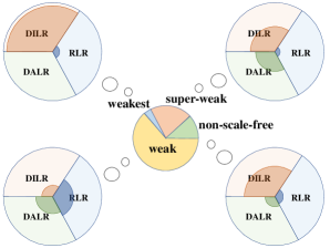
Figure 5: Probabilities of adversarial networks to belong to different categories. The middle pie chart represents the overall results by considering all the cases (three attack strategies on all the networks of different sizes). The surrounding pies represent the probabilities of the adversarial networks generated by different attack strategies for each category.

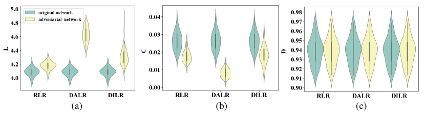
Figure 6: The violin plots of the three structural properties, $L$, $C$ and $D$, of the networks both before and after the attacks by different strategies.

First, it seems that the probabilities of the adversarial networks (obtained by attacking strong scale-free networks) belonging to different categories are quite different. Overall, by considering all the cases (three attack strategies on the networks of different sizes), the adversarial networks are most likely to be in the weak category (with probability 62.92%), but are most difficult to be in the weakest category (with probability 1.75%), as shown in Fig. 5. By comparison, the adversarial networks are relatively easier to be in the super-weak category, rather than in the non-scale-free category, with properties 23.96% and 11.37%, respectively. This is because, generally, it is quite costly (a large number of links need to be rewired) to make $n_{tail}$ less than 50, especially for those networks of large sizes, where $n_{tail}\leq{50}$ is the threshold to define the weakest category. On the contrary, the other three parameters, $\alpha$, $R$ and $p$, are more sensitive to the attacks, since they are determined by the overall curve of the degree distribution, especially for the first two. Note that the fractions of adversarial networks in different categories are slightly different by attacks of different strategies, e.g., most of the adversarial networks in the weak category are generated by RLR, while most of those in the other three categories (weakest, super-weak, non-scale-free) are generated by DILR. But, overall, these strategies are consistent with each other.

Second, the two heuristic attack strategies are much more effective than the random rewiring strategy RLR, in the sense that a smaller $\Delta{M}$ is needed to succeed in the attack, while among them DILR is the most effective one. As shown in TABLE 3, for RLR, which can be considered as random noise, typically more than 15% links in the original networks need to be rewired to succeed in the attack (from strong to weak, weakest, or super-weak). However, surprisingly, only around 5% links need to be rewired when the network is attacked to become non-scale-free, although such cases are rare. This result suggests that the BC classification could be robust against small random noise. More interestingly, when the perturbations are purposefully designed, the BC classification will be quite vulnerable, i.e., only 3.89% links (38.9 in 1000 links on average) need to be rewired if DILR is applied to attack the networks of 500 nodes, much less than the value of 17.30% by RLR. It seems that, as the network size increases, it is more difficult to succeed in an attack, e.g., the fractions of rewired links for both DALR and DILR steadily increases as the network size increases. Even so, the number of rewired links needed by DALR or DILR is only half of those needed by RLR, when the networks have 2000 nodes and 4000 links. By comparison, DILR is generally more effective than DALR, i.e., a smaller number of links are needed to succeed in attack when DILR is applied rather than DALR.

Third, the adversarial attack will not change the network structure by too much, i.e., the relative changes of $L$, $C$, and $D$ introduced by DILR are comparable with those introduced by RLR. It is well known that the average shortest path-length $L$ and the average clustering coefficient $C$ are good for characterizing the global and local properties, respectively. On the other hand, the recently proposed diagonal distance $D$ is also a global property useful for detecting the dramatic changes in the topology of a network Tsiotas (2019). Here, the relative changes of these three properties are used, i.e., $\Delta{L}$, $\Delta{C}$, and $\Delta{D}$, between the original networks and the adversarial networks, to measure if these properties will dramatically change under adversarial attacks. The results are presented in TABLE 4. It is found that, overall, $\Delta{L}$ introduced by DILR is larger than those introduced by RLR, but much smaller than that introduced by DALR, and that DILR and RLR have comparable $\Delta{C}$, around 30%, which is only half of that introduced by DALR. All the three attack strategies introduce very small $\Delta{D}$, i.e., lower than 1%. Note that, here $\Delta{C}$ is relatively large for all the three attack strategies, because BA scale-free networks do not have many triangular motifs, thus have very small average clustering coefficients. Consequently, a very small perturbation on a triangular structure will lead to a huge change of $\Delta{C}$ according to Eq. (8). To statistically compare the original networks and the adversarial networks generated by each attack strategy, the violin plots is shown for the three structural properties, i.e., $L$, $C$ and $D$, of the networks, both before and after an attack, as shown in Fig. 6. It is found that the shortest path-length increases and the clustering coefficient decreases after the attack, while the diagonal distance remains almost the same. This is reasonable, since the attack focuses on destroying the scale-free property, which will weaken the dominant role of hub nodes and further increase the shortest path-length. On the other hand, the global random rewiring operations in the three strategies may also destruct triangles in these networks, leading to smaller clustering coefficients. In general, DILR has comparable concealment as RLR, both of which introduce relatively small changes of $L$, $C$ and $D$; while DALR causes dramatic changes of the network structures, thus could be relatively easy to detect.

V Conclusion

This paper has discussed the robustness of the scale-free network classification method proposed by Broido and Clauset Broido and Clauset (2019), referred to as BC classification herein. In so doing, three attack strategies, RLR, DALR and DILR, are proposed and tested. The attack experiments on strong scale-free networks generated by the BA model show that the BC classification method is vulnerable to adversarial attacks, e.g., only 6% links need to be rewired to successfully attack a strong scale-free network such that it becomes a weak, weakest, super-weak, or even non-scale-free network. In addition, the BC classification result is not as good as described Broido and Clauset (2019): The cost of transforming a strong network into the weakest category is even higher than the cost of transforming it into the non-scale-free category, which indicates that there is no layered relationship between these categories.

This paper has examined four indicators in the BC classification method: $p$, $n_{tail}$, $R$, and $\alpha$. Among these indicators, the values of $p$ and $\alpha$ can be easily changed by slightly disturbing the network structure, while $n_{tail}$ and $R$ show relatively strong robustness. This results in unbalanced distributions of the adversarial networks in different categories. For instance, since the requirement of the weakest category is $n_{tail}>50$, it is extremely difficult to attack a strong scale-free network to change it to be in the weakest category, especially when the network is relatively large. Therefore, one should consider the robustness for each indicator when trying to propose a new classification method.

This study may provide a different perspective to the arguable definition of scale-free networks. Moreover, beyond the scale-free feature, in complex networks there are also many other physical criteria derived from real-world data. Therefore, a suggestion is to adopt similar methods to test their robustness against various adversarial attacks.

References

- Ebel, Mielsch, and Bornholdt (2002) H. Ebel, L.-I. Mielsch, and S. Bornholdt, “Scale-free topology of e-mail networks,” Physical review E 66, 035103 (2002).
- Albert (2005) R. Albert, “Scale-free networks in cell biology,” Journal of Cell Science 118, 4947–4957 (2005).
- Albert, Jeong, and Barabási (1999) R. Albert, H. Jeong, and A.-L. Barabási, “Internet: Diameter of the world-wide web,” Nature 401, 130 (1999).
- Xuan et al. (2019) Q. Xuan, J. Wang, M. Zhao, J. Yuan, C. Fu, Z. Ruan, and G. Chen, “Subgraph networks with application to structural feature space expansion,” IEEE Transactions on Knowledge and Data Engineering (2019).
- Barabási and Albert (1999) A.-L. Barabási and R. Albert, “Emergence of scaling in random networks,” Science 286, 509–512 (1999).
- Barabási, Albert, and Jeong (1999) A.-L. Barabási, R. Albert, and H. Jeong, “Mean-field theory for scale-free random networks,” Physica A: Statistical Mechanics and its Applications 272, 173–187 (1999).
- Molontay and Nagy (2020) R. Molontay and M. Nagy, “Twenty years of network science: A bibliographic and co-authorship network analysis,” arXiv2001.09006 (2020).
- Dorogovtsev and Mendes (2002) S. N. Dorogovtsev and J. F. Mendes, “Evolution of networks,” Advances in physics 51, 1079–1187 (2002).
- Willinger, Alderson, and Doyle (2009) W. Willinger, D. Alderson, and J. C. Doyle, “Mathematics and the internet: A source of enormous confusion and great potential,” Notices of the American Mathematical Society 56, 586–599 (2009).
- Broido and Clauset (2019) A. D. Broido and A. Clauset, “Scale-free networks are rare,” Nature Communications 10, 1017 (2019).
- Barabási (2018) A. Barabási, “Love is all you need: Clauset’s fruitless search for scale-free networks,” Blog post available at https://www. barabasilab. com/post/love-is-all-you-need (2018).
- Voitalov et al. (2018) I. Voitalov, P. van der Hoorn, R. van der Hofstad, and D. Krioukov, “Scale-free networks well done,” arXiv preprint arXiv:1811.02071 (2018).
- Szegedy et al. (2013) C. Szegedy, W. Zaremba, I. Sutskever, J. Bruna, D. Erhan, I. Goodfellow, and R. Fergus, “Intriguing properties of neural networks,” arXiv preprint arXiv:1312.6199 (2013).
- Xuan et al. (2017a) Q. Xuan, B. Fang, Y. Liu, J. Wang, J. Zhang, Y. Zheng, and G. Bao, “Automatic pearl classification machine based on a multistream convolutional neural network,” IEEE Transactions on Industrial Electronics 65, 6538–6547 (2017a).
- Xuan et al. (2018) Q. Xuan, Z. Chen, Y. Liu, H. Huang, G. Bao, and D. Zhang, “Multiview generative adversarial network and its application in pearl classification,” IEEE Transactions on Industrial Electronics 66, 8244–8252 (2018).
- Papernot et al. (2016) N. Papernot, P. McDaniel, S. Jha, M. Fredrikson, Z. B. Celik, and A. Swami, “The limitations of deep learning in adversarial settings,” in 2016 IEEE European Symposium on Security and Privacy (EuroS&P) (IEEE, 2016) pp. 372–387.
- Su, Vargas, and Sakurai (2019) J. Su, D. V. Vargas, and K. Sakurai, “One pixel attack for fooling deep neural networks,” IEEE Transactions on Evolutionary Computation (2019).
- Moosavi-Dezfooli, Fawzi, and Frossard (2016) S.-M. Moosavi-Dezfooli, A. Fawzi, and P. Frossard, “Deepfool: a simple and accurate method to fool deep neural networks,” in Proceedings of the IEEE Conference on Computer Vision and Pattern Recognition (2016) pp. 2574–2582.
- Xie et al. (2017) C. Xie, J. Wang, Z. Zhang, Y. Zhou, L. Xie, and A. Yuille, “Adversarial examples for semantic segmentation and object detection,” in Proceedings of the IEEE International Conference on Computer Vision (2017) pp. 1369–1378.
- Goodfellow, Shlens, and Szegedy (2014) I. J. Goodfellow, J. Shlens, and C. Szegedy, “Explaining and harnessing adversarial examples,” arXiv preprint arXiv:1412.6572 (2014).
- Kurakin, Goodfellow, and Bengio (2016) A. Kurakin, I. Goodfellow, and S. Bengio, “Adversarial examples in the physical world,” arXiv preprint arXiv:1607.02533 (2016).
- Moosavi-Dezfooli et al. (2017) S.-M. Moosavi-Dezfooli, A. Fawzi, O. Fawzi, and P. Frossard, “Universal adversarial perturbations,” in Proceedings of the IEEE Conference on Computer Vision and Pattern Recognition (2017) pp. 1765–1773.
- Dai et al. (2018) H. Dai, H. Li, T. Tian, X. Huang, L. Wang, J. Zhu, and L. Song, “Adversarial attack on graph structured data,” arXiv preprint arXiv:1806.02371 (2018).
- Fu et al. (2018) C. Fu, M. Zhao, L. Fan, X. Chen, J. Chen, Z. Wu, Y. Xia, and Q. Xuan, “Link weight prediction using supervised learning methods and its application to yelp layered network,” IEEE Transactions on Knowledge and Data Engineering 30, 1507–1518 (2018).
- Chen et al. (2019a) J. Chen, J. Zhang, X. Xu, C. Fu, D. Zhang, Q. Zhang, and Q. Xuan, “E-lstm-d: A deep learning framework for dynamic network link prediction,” IEEE Transactions on Systems, Man, and Cybernetics: Systems (2019a).
- Wang et al. (2018) X. Wang, J. Eaton, C.-J. Hsieh, and F. Wu, “Attack graph convolutional networks by adding fake nodes,” arXiv preprint arXiv:1810.10751 (2018).
- Chen et al. (2019b) J. Chen, L. Chen, Y. Chen, M. Zhao, S. Yu, Q. Xuan, and X. Yang, “Ga-based q-attack on community detection,” IEEE Transactions on Computational Social Systems 6, 491–503 (2019b).
- Yu et al. (2019) S. Yu, M. Zhao, C. Fu, J. Zheng, H. Huang, X. Shu, Q. Xuan, and G. Chen, “Target defense against link-prediction-based attacks via evolutionary perturbations,” IEEE Transactions on Knowledge and Data Engineering (2019).
- Zügner, Akbarnejad, and Günnemann (2018) D. Zügner, A. Akbarnejad, and S. Günnemann, “Adversarial attacks on neural networks for graph data,” in Proceedings of the 24th ACM SIGKDD International Conference on Knowledge Discovery & Data Mining (ACM, 2018) pp. 2847–2856.
- Evans, Mills, and Dawson (1988) S. Evans, P. Mills, and J. Dawson, “The end of the p value?” British Heart Journal 60, 177 (1988).
- Amrhein, Greenland, and McShane (2019) V. Amrhein, S. Greenland, and B. McShane, “Scientists rise up against statistical significance,” (2019).
- Gerlach and Altmann (2019) M. Gerlach and E. G. Altmann, “Testing statistical laws in complex systems,” Physical Review Letters 122, 168301 (2019).
- Albert, Jeong, and Barabási (2000) R. Albert, H. Jeong, and A.-L. Barabási, “Error and attack tolerance of complex networks,” Nature 406, 378 (2000).
- Pastor-Satorras, Vespignani et al. (2003) R. Pastor-Satorras, A. Vespignani, et al., “Epidemics and immunization in scale-free networks,” Handbook of Graphs and Networks, Wiley-VCH, Berlin (2003).
- Ruan, Tang, and Liu (2012) Z. Ruan, M. Tang, and Z. Liu, “Epidemic spreading with information-driven vaccination,” Physical Review E 86, 036117 (2012).
- Wolfson et al. (2009) M. Wolfson, A. Budovsky, R. Tacutu, and V. Fraifeld, “The signaling hubs at the crossroad of longevity and age-related disease networks,” International Journal of Biochemistry Cell Biology 41, 516–520 (2009).
- Wang and Chen (2002) X. F. Wang and G. Chen, “Pinning control of scale-free dynamical networks,” Physica A: Statistical Mechanics and its Applications 310, 521–531 (2002).
- Xuan et al. (2017b) Q. Xuan, Z.-Y. Zhang, C. Fu, H.-X. Hu, and V. Filkov, “Social synchrony on complex networks,” IEEE transactions on cybernetics 48, 1420–1431 (2017b).
- Bianconi and Barabási (2001) G. Bianconi and A.-L. Barabási, “Bose-einstein condensation in complex networks,” Physical Review Letters 86, 5632 (2001).
- Li and Chen (2003) X. Li and G. Chen, “A local-world evolving network model,” Physica A 328, 287–296 (2003).
- Xuan, Li, and Wu (2006) Q. Xuan, Y. Li, and T.-J. Wu, “Growth model for complex networks with hierarchical and modular structures,” Physical Review E 73, 036105 (2006).
- Xuan, Li, and Wu (2007) Q. Xuan, Y. Li, and T.-J. Wu, “A local-world network model based on inter-node correlation degree,” Physica A: Statistical Mechanics and its Applications 378, 561–572 (2007).
- Sen and Dai (2009) Q. Sen and G.-Z. Dai, “A new local-world evolving network model,” Chinese Physics B 18, 383 (2009).
- Ugander et al. (2011) J. Ugander, B. Karrer, L. Backstrom, and C. Marlow, “The anatomy of the facebook social graph,” arXiv preprint arXiv:1111.4503 (2011).
- Watts and Strogatz (1998) D. J. Watts and S. H. Strogatz, “Collective dynamics of ’small-world’ networks,” Nature 393, 440 (1998).
- Tsiotas (2019) D. Tsiotas, “Detecting different topologies immanent in scale-free networks with the same degree distribution,” Proceedings of the National Academy of Sciences 116, 6701–6706 (2019).