Combined search for anisotropic birefringence in the gravitational-wave transient catalog GWTC-1

Abstract

The discovery of gravitational waves (GWs) provides an unprecedented arena to test general relativity, including the gravitational Lorentz invariance violation (gLIV). In the propagation of GWs, a generic gLIV leads to anisotropy, dispersion, and birefringence. GW events constrain the anisotropic birefringence particularly well. Kostelecký and Mewes (2016) performed a preliminary analysis for GW150914. We improve their method and extend the analysis systematically to the whole GW transient catalog, GWTC-1. This is the first global analysis of the spacetime anisotropic Lorentzian structure with a catalog of GWs, where multiple events are crucial in breaking the degeneracy among gLIV parameters. With the absence of abnormal propagation, we obtain new limits on 34 coefficients for gLIV in the nonminimal gravity that surpass previous limits by $\sim 10^{2}$–$10^{5}$.

I Introduction

Lorentz invariance is a cherished symmetry laying to the heart of modern physics. However, motivated by contemporary open questions, there are good reasons to believe that, the Lorentz symmetry breaks at some yet unknown energy scale Jacobson et al. (2006); Tasson (2014). For example, in the string theory it is perceived to have a Higgs-like spontaneous symmetry breaking of the Lorentz invariance Kostelecký and Samuel (1989); Kostelecký and Potting (1991) which leads to various observable phenomena Mattingly (2005); Kostelecký and Russell (2011). While the Lorentz invariance violation (LIV) in principle happens in different species sectors Carroll et al. (1990); Colladay and Kostelecký (1997, 1998), it is the most interesting to study the gravitational LIV (gLIV) due to the following fact Kostelecký (2004); Hees et al. (2016); Shao and Wex (2016); Tasson (2016). Up to now, the canonical theory of gravitation, namely the general relativity, while being extremely faithful in describing various gravity experiments Will (2014); Berti et al. (2015), still refuses to embed into the framework of quantum field theory which successfully describes the other three fundamental interactions in a unified way. Therefore, searches for gLIV are closely linked to searches for quantum-gravity candidate theories Amelino-Camelia et al. (1998); Gambini and Pullin (1999); Amelino-Camelia (2013); Berti et al. (2015).

Nowadays the most popular framework to investigate the possibility of gLIV is the standard-model extension (SME) Kostelecký (2004) and the parameterized post-Newtonian formalism Will (2014, 2018). We will focus on the former. The SME is an agnostic effective field theory which incorporates all gauge-preserving, Lorentz-violating, energy-momentum-conserving operators that are constructed from the field operators in general relativity and particle physics. New Lorentz-covariant operators are built from contraction of known fields with LIV coefficients. Unless being protected, operators with lower mass dimension are expected to dominate the observables as per the spirit of effective field theories. Here we focus on the subset of the SME that deals with the pure gravity sector; interested readers are referred to Ref. Kostelecký and Tasson (2011) for discussions on the matter-gravity couplings. In an effective-field-theoretic framework, to be compatible with the Riemann-Cartan geometry, the symmetry breaking shall be spontaneous instead of explicit Bluhm and Kostelecký (2005). Therefore the SME, while being particle Lorentz-violating, is observer Lorentz-invariant.

The convenience in using the SME to test the Lorentz symmetry has resulted in a flourish of studies during the past decades from different kinds of experiments concerning various particle species Kostelecký and Russell (2011). For the gravity sector, constraints come from lunar laser ranging Battat et al. (2007); Bourgoin et al. (2017), atom interferometers Mueller et al. (2008), cosmic rays Kostelecký and Tasson (2015), precision pulsar timing Shao (2014a, b); Jennings et al. (2015); Shao and Bailey (2018, 2019); Shao (2019), planetary orbital dynamics Hees et al. (2015), laboratory short-range experiments Bailey et al. (2015); Shao et al. (2016); Kostelecký and Mewes (2017); Shao et al. (2019), super-conducting gravimeters Flowers et al. (2017), and recently gravitational waves (GWs) Kostelecký and Mewes (2016); Mewes (2019); Xu et al. (2020); see Hees et al. (2016) for a comprehensive review. These constraints are complementary to each other, and in many cases they are individually competent at probing different parts of the parameter space. For example, timing of binary pulsars was shown to be good at systematically probing the lowest-order CPT-violating Bailey and Havert (2017); Shao and Bailey (2018), as well as gravitational weak-equivalence-principle-violating Bailey (2016); Shao and Bailey (2019), operators via the post-Newtonian dynamics, while laboratory short-range experiments excel in constraining the nonminimal operators in a static Newtonian setup Kostelecký and Mewes (2017).

A newly emerging probe to gLIV phenomena in gravity is the recently discovered GWs by the Advanced LIGO/Virgo detectors Abbott et al. (2016); Kostelecký and Mewes (2016); Abbott et al. (2019a). The propagation of GWs has become one of the central topics in looking for gLIV clues Will (1998); Mirshekari et al. (2012); Yunes et al. (2016); Abbott et al. (2017a); Nishizawa (2018); Arai and Nishizawa (2018); Wang (2017); Qiao et al. (2019); Zhao et al. (2020); Wang and Zhao (2020). The existence of gLIV would generally cause anisotropy, dispersion, and birefringence Kostelecký and Mewes (2016); Mewes (2019). Following the theoretical work by Will (1998) and Mirshekari et al. (2012), the LIGO/Virgo Collaboration have conducted extensive tests of the GW dispersion relation caused by the gLIV or a massive graviton Abbott et al. (2017a, 2019b). However, most of the past study focused on the boost breaking, and ignored the breaking of the rotational symmetry. While the commutator of two boost generators gives a rotation generator, it is inevitable to host the rotation breaking when the boost symmetry is broken, unless the object under investigation is exactly at rest with respect to a preferred frame. Such a preferred frame may not even exist in effective field theories K. Nordtvedt (1976); Bailey and Kostelecký (2006). This motivates us to look at the anisotropic gLIV and test it thereof in a more generic way.

In this work we follow the preliminary analysis done by Kostelecký and Mewes (2016), and extend it systematically with all the GW events detected in the first and second observing runs Abbott et al. (2019a). It is the first study of this kind, and probes the gLIV with a globally coherent approach. Using the fact that the SME is observer Lorentz-invariant, we combine different GW events from the GW transient catalog, GWTC-1 Abbott et al. (2019a), including ten binary black holes (BBHs) and one binary neutron star (BNS), GW 170817 Abbott et al. (2017b); see Appendix A for basic parameters of GW events in the GWTC-1. A global analysis with the basis of spin-weighted spherical harmonics provides us new limits on the gLIV coefficients in the nonminimal gravity at mass dimensions 5 and 6. These limits are orders of magnitude tighter than the existing ones. GW observations truly represent precious treasures in studying various gravity theories. While more detections are continuously being made, the investigation in this paper will be improved dramatically and new clues to quantum gravity might be drawn.

The paper is organized as follows. In the next section, we briefly discuss the modified dispersion relation for the linearized gravity in SME, and its effect on the cosmological GW propagation. Anisotropic birefringent effects can be constrained particularly well with GWs. Therefore we focus on the anisotropic birefringence in Sec. III, and lay down the strategies for the practical application to the GWTC-1. In Sec. IV we present detailed Monte Carlo analysis using the posteriors on the GW parameters for the 11 events in the catalog, provided by the LIGO/Virgo Collaboration. Numerical constraints on 34 gLIV coefficients are obtained with the maximal-reach Tasson (2019) and global approaches. The global analysis, simultaneously with tens of gLIV parameters analyzed, is done for the first time with GWs in a coherent way. It greatly extends previous work done by the LIGO/Virgo Collaboration Abbott et al. (2017a, 2019c, 2019b) and Kostelecký and Mewes (2016). Finally, Sec. V summarizes the paper and discusses future directions for improvement. For readers’ convenience, extra information on the GWTC-1 catalog, the spin-weighted spherical harmonics, and a fitting formula to the GW peak frequency are provided respectively in Appendices A, B, and C.

Throughout the paper, we follow conventions used by Misner et al. (1973) and Kostelecký (2004). Unless otherwise stated, we use natural units where $\hbar=G=c=1$.

II Dispersion and propagation of gravitational waves

The gravity sector in the SME was given fully in the Riemann-Cartan spacetime Kostelecký (2004). However, we restrict ourselves to a 4-dimensional Riemannian spacetime, and only consider the part of spacetime where, after fixing the gauge, the linearized gravity is a sufficiently good approximation. The metric, $g_{\mu\nu}=\eta_{\mu\nu}+h_{\mu\nu}$, is expanded around the Minkowski metric, $\eta_{\mu\nu}$, with a perturbation, $h_{\mu\nu}$. Kostelecký and Mewes (2016) constructed the general quadratic Lagrangian density for GWs in the presence of gLIV operators of arbitrary mass dimension $d$,

$${\cal L}_{{\cal K}^{(d)}}=\frac{1}{4}h_{\mu\nu}\hat{\cal K}^{(d)\mu\nu\rho\sigma}h_{\rho\sigma}\,,$$ (1)

where $\hat{\cal K}^{(d)\mu\nu\rho\sigma}={\cal K}^{(d)\mu\nu\rho\sigma i_{1}i_{2}\cdots i_{d-2}}\partial_{i_{1}}\partial_{i_{2}}\cdots\partial_{i_{d-2}}$ with the “hat” denoting its operator nature, and ${\cal K}^{(d)\mu\nu\rho\sigma i_{1}i_{2}\cdots i_{d-2}}$ are normal tensorial components whose mass dimension is $4-d$.

With the help of the Young tableaux, Kostelecký and Mewes (2016, 2018) studied the irreducible decomposition of the operator $\hat{\cal K}^{(d)\mu\nu\rho\sigma}$ thoroughly. They found that three classes of operators are invariant under the infinitesimal gauge transformation $h_{\mu\nu}\rightarrow h_{\mu\nu}+\partial_{\mu}\xi_{\nu}+\partial_{\nu}\xi_{\mu}$. Imposing such a gauge symmetry, one arrives at a complete gauge-invariant quadratic Lagrangian density,

$${\cal L}={\cal L}_{0}+\frac{1}{4}h_{\mu\nu}\left(\hat{s}^{\mu\rho\nu\sigma}+\hat{q}^{\mu\rho\nu\sigma}+\hat{k}^{\mu\nu\rho\sigma}\right)h_{\rho\sigma}\,,$$ (2)

where ${\cal L}_{0}=\frac{1}{4}\epsilon^{\mu\rho\alpha\kappa}\epsilon^{\nu\sigma\beta\lambda}\eta_{\kappa\lambda}h_{\mu\nu}\partial_{\alpha}\partial_{\beta}h_{\rho\sigma}$ is the linearized Einstein-Hilbert Lagrangian. Operators $\hat{s}^{\mu\rho\nu\sigma}$, $\hat{q}^{\mu\rho\nu\sigma}$, and $\hat{k}^{\mu\nu\rho\sigma}$ are the sums over $d$ of each of three irreducible sets; see Table 1 and Eq. (3) in Ref. Kostelecký and Mewes (2016) for their relations to $\hat{\cal K}^{(d)\mu\nu\rho\sigma}$. These operators have the following symmetries:

1. $\hat{s}^{\mu\rho\nu\sigma}$ is anti-symmetric in both “$\mu\rho$” and “$\nu\sigma$”;

2. $\hat{q}^{\mu\rho\nu\sigma}$ is anti-symmetric in “$\mu\rho$” and symmetric in “$\nu\sigma$”;

3. $\hat{k}^{\mu\nu\rho\sigma}$ is totally symmetric.

In addition, any contraction of these operators with a derivative is zero.

Similar to the previous study in the photon sector of the electrodynamic SME Kostelecký and Mewes (2002, 2009), the covariant dispersion relation for the two tensor modes of a GW with 4-momentum $p^{\mu}=\left(\omega,\bm{p}\right)$ is Kostelecký and Mewes (2016),

$$\omega=\left(1-\zeta^{0}\pm\sqrt{\left(\zeta^{1}\right)^{2}+\left(\zeta^{2}\right)^{2}+\left(\zeta^{3}\right)^{2}}\right)p\,,$$ (3)

where

$$\zeta^{0}=\frac{1}{4p^{2}}\left(-\tensor{\hat{s}}{{}^{\mu\nu}_{\mu\nu}}+\frac{1}{2}\tensor{\hat{k}}{{}^{\mu\nu}_{\mu\nu}}\right)\,,$$ (4)

$$\left(\zeta^{1}\right)^{2}+\left(\zeta^{2}\right)^{2}=\frac{1}{8p^{4}}\left(\hat{k}^{\mu\nu\rho\sigma}\hat{k}_{\mu\nu\rho\sigma}-\tensor{\hat{k}}{{}^{\mu\rho}_{\nu\rho}}\tensor{\hat{k}}{{}_{\mu\sigma}^{\nu\sigma}}+\frac{1}{8}\tensor{\hat{k}}{{}^{\mu\nu}_{\mu\nu}}\tensor{\hat{k}}{{}^{\rho\sigma}_{\rho\sigma}}\right)\,,$$ (5)

$$\left(\zeta^{3}\right)^{2}=\frac{1}{16p^{4}}\left[\left(\tensor{\hat{q}}{{}^{\mu\rho\nu}_{\rho}}+\tensor{\hat{q}}{{}^{\nu\rho\mu}_{\rho}}\right)\tensor{\hat{q}}{{}_{\mu\sigma\nu}^{\sigma}}-\frac{1}{2}\hat{q}^{\mu\rho\nu\sigma}\hat{q}_{\mu\rho\nu\sigma}-\hat{q}^{\mu\nu\rho\sigma}\hat{q}_{\mu\rho\nu\sigma}\right]\,.$$ (6)

Here the decomposition is done by the handedness of GWs, instead of the usual “$+$” and “$\times$” modes. In above equations, $\zeta^{0}$ and $\zeta^{3}$ are rotation scalars, $\zeta^{1}$ and $\zeta^{2}$ are helicity-4 tensors, and the derivative “$\partial_{\mu}$” in operators is understood to be replaced by “$ip_{\mu}$” Kostelecký and Mewes (2016).

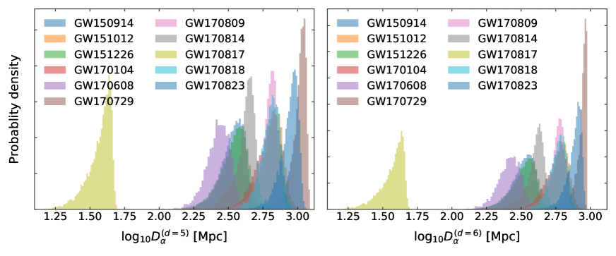
Figure 1: Probability density for $D_{\alpha}^{(d=5)}$ and $D_{\alpha}^{(d=6)}$, derived using the posterior samples provided by the LIGO/Virgo Collaboration Abbott et al. (2019a); GWT (a, b).

To report experimental constraints on the coefficients for Lorentz/CPT violation in the SME, it is conventional to use the canonical Sun-centered celestial-equatorial frame Kostelecký and Mewes (2002). Concerning the rotational behavior, it is useful to decompose $\zeta^{\alpha}$ with spin-weighted spherical harmonics Kostelecký and Mewes (2009, 2016),

$$\zeta^{0} = \sum_{djm}\omega^{d-4}Y_{jm}\left(\hat{\bm{n}}\right)k^{(d)}_{(I)jm}\,,$$ (7)

$$\zeta^{1}\mp i\zeta^{2} = \sum_{djm}\omega^{d-4}{}_{\pm 4}Y_{jm}\left(\hat{\bm{n}}\right)\left[k^{(d)}_{(E)jm}\pm ik^{(d)}_{(B)jm}\right]\,,$$ (8)

$$\zeta^{3} = \sum_{djm}\omega^{d-4}Y_{jm}\left(\hat{\bm{n}}\right)k^{(d)}_{(V)jm}\,,$$ (9)

where $\hat{\bm{n}}\equiv-\hat{\bm{p}}$ is the direction to the source, and $|s|\leq j\leq d-2$; see Appendix B for more details on the spin-weighted spherical harmonics. It was shown that Kostelecký and Mewes (2016),

1. anisotropic effects are governed by the coefficients with $j\neq 0$;

2. frequency-dependent dispersions are governed by all coefficients except $k^{(4)}_{(I)jm}$;

3. vacuum birefringent effects are governed by all coefficients except $k^{(d)}_{(I)jm}$.

Besides, $d\geq 4$ is even for $k^{(d)}_{(I)jm}$; $d\geq 5$ is odd for $k^{(d)}_{(V)jm}$; and $d\geq 6$ is even for $k^{(d)}_{(E)jm}$ and $k^{(d)}_{(B)jm}$.

Assuming that the corrections to Einstein’s general relativity are small, we obtain the phase speed of GWs from Eq. (3), $v_{\rm GW}=\omega/p=1-\zeta^{0}\pm\sqrt{\sum_{i=1}^{3}\left(\zeta^{i}\right)^{2}}$. In accordance to the spirit of effective field theories, we further assume that the gLIV happens dominantly at a specific mass dimension $d$. If it had happened at multiple dimensions, we equivalently take the dimension $d$, usually the lowest relevant mass dimension where gLIV happens, which introduces the maximum effect. By this assumption we ease the summation over “$d$” in Eqs. (7–9), and denote the original $\zeta^{\alpha}$ as $\zeta^{\alpha}_{(d)}$ ($\alpha=0,1,2,3$). Further, we introduce a notation, $\tilde{\zeta}^{\alpha}_{(d)}\left(\hat{\bm{n}}\right)\equiv\zeta^{\alpha}_{(d)}\left(\hat{\bm{n}}\right)\times\omega^{4-d}$ which are energy-independent; for example, $\tilde{\zeta}^{0}_{(d)}\left(\hat{\bm{n}}\right)=\sum_{jm}Y_{jm}\left(\hat{\bm{n}}\right)k^{(d)}_{(I)jm}$. With these considerations, the speed of GWs simplifies to,

$$v_{\rm GW}^{(d)}=1-\omega^{d-4}\left\{\tilde{\zeta}^{0}_{(d)}\mp\sqrt{\sum_{i=1}^{3}\left(\tilde{\zeta}^{i}_{(d)}\right)^{2}}\right\}\,,$$ (10)

where an important fact is that the terms inside the curly bracket is, while being direction-dependent, energy-independent.

Table 1: In the table we show (i) the GW peak frequency $f_{\rm GW}$ at the merger using the fit in Eq. (18), and (ii) the distance-like quantity, $D_{\alpha}^{(d)}$, defined in Eq. (12), for mass dimensions $d=5$ and $d=6$. The uncertainties are given at the $90\%$ confidence level. Notice that, because the merger part for the BNS was not observed Abbott et al. (2017b, 2019d), in our test we conservatively use $f_{\rm GW}=800$ Hz for GW170817.

	$f_{\rm GW}$ [Hz]	$D_{\alpha}^{(d=5)}$ [Mpc]	$D_{\alpha}^{(d=6)}$ [Mpc]
GW150914	$174_{-7}^{+6}$	$350_{-120}^{+90}$	$330_{-110}^{+80}$
GW151012	$307_{-68}^{+35}$	$660_{-220}^{+170}$	$610_{-190}^{+140}$
GW151226	$547_{-122}^{+45}$	$350_{-130}^{+110}$	$340_{-120}^{+100}$
GW170104	$220_{-22}^{+18}$	$620_{-200}^{+150}$	$570_{-180}^{+120}$
GW170608	$619_{-97}^{+25}$	$270_{-80}^{+80}$	$260_{-80}^{+70}$
GW170729	$146_{-21}^{+18}$	$1050_{-260}^{+120}$	$890_{-180}^{+60}$
GW170809	$196_{-18}^{+12}$	$640_{-180}^{+110}$	$580_{-160}^{+90}$
GW170814	$209_{-10}^{+7}$	$430_{-130}^{+90}$	$410_{-120}^{+70}$
GW170817	$4243_{-81}^{+24}$	$39_{-14}^{+6}$	$38_{-14}^{+6}$
GW170818	$180_{-14}^{+12}$	$650_{-170}^{+150}$	$590_{-140}^{+120}$
GW170823	$169_{-20}^{+17}$	$900_{-250}^{+150}$	$790_{-190}^{+100}$

Now consider two gravitons emitted at $t_{e}$ and $t_{e}^{\prime}$ with energies $\omega_{e}$ and $\omega^{\prime}_{e}$ respectively. After traveling over a same comoving distance Will (1998); Jacob and Piran (2008); Mirshekari et al. (2012), they arrive at a GW detector on the Earth at $t_{a}$ and $t_{a}^{\prime}$. Following the method developed by Will (1998) and Mirshekari et al. (2012), we derive

$$\Delta t_{a}=(1+z)\left\{\Delta t_{e}+\Delta\omega_{e}^{d-4}D_{\alpha}^{(d)}\left[\tilde{\zeta}^{0}_{(d)}\mp\sqrt{\sum_{i=1}^{3}\left(\tilde{\zeta}^{i}_{(d)}\right)^{2}}\right]\right\}\,,$$ (11)

where $\Delta t_{e}\equiv t_{e}-t_{e}^{\prime}$, $\Delta t_{a}\equiv t_{a}-t_{a}^{\prime}$, $\Delta\omega_{e}^{d-4}\equiv\omega_{e}^{d-4}-{\omega_{e}^{\prime}}^{d-4}$, and $z$ is the cosmological redshift. A new distance-like quantity in the above equation is defined as Will (1998),

$$D_{\alpha}^{(d)}\equiv\frac{\left(1+z\right)^{3-d}}{H_{0}}\int_{0}^{z}\frac{\left(1+z^{\prime}\right)^{d-4}}{\sqrt{\Omega_{m}\left(1+z^{\prime}\right)^{3}+\Omega_{\Lambda}}}{\rm d}z^{\prime}\,,$$ (12)

where $H_{0}=\left(67.4\pm 0.5\right)\,{\rm km}\,{\rm s}^{-1}\,{\rm Mpc}^{-1}$ is the Hubble constant, $\Omega_{m}=0.315\pm 0.007$ is the fraction of matter energy density, and $\Omega_{\Lambda}=0.685\pm 0.007$ is the fraction of vacuum energy density in our current Universe Aghanim et al. (2018). We have used the standard $\Lambda$CDM model, which should be rather precise for the GW events with relatively low redshifts. For the 11 GW events in the GWTC-1, their $D_{\alpha}^{(d)}$ for $d=5$ and $d=6$ are given in Fig. 1 and Table 1.

III Constraining anisotropic birefringence

The modified dispersion relation (3) introduces anisotropy, dispersion, and birefringence to the propagation of GWs Kostelecký and Mewes (2016). As the first application, Kostelecký and Mewes (2016) used the observation that there is no indication of mode splitting at the amplitude peak of GW150914 Abbott et al. (2016). They took a rough value for the upper limit of the time difference for the arrival of two circular modes, $\Delta t\leq 3$ ms, and used a central frequency $f\sim 100$ Hz, to derive the limit on the difference in the propagation speed between the two circularly polarized CPT-conjugate eigenmodes. They obtained the first constraint on the gLIV in the pure-gravity sector with $d=5$,

$$\left|\sum_{jm}Y_{jm}\left(\theta,\phi\right)k^{(5)}_{(V)jm}\right|\leq 2\times 10^{-14}\,{\rm m}\,,$$ (13)

and a competitive limit to existing laboratory bounds on birefringent coefficients at $d=6$,

$$\left|\sum_{jm}{}_{\pm 4}Y_{jm}\left(\theta,\phi\right)\left(k^{(6)}_{(E)jm}\pm ik^{(6)}_{(B)jm}\right)\right|\leq 8\times 10^{-9}\,{\rm m}^{2}\,,$$ (14)

for $\theta\simeq 160^{\circ}$ and $\phi\simeq 120^{\circ}$ Kostelecký and Mewes (2016), where $(\theta,\phi)$ is the (very) rough sky position of GW150914 in the Sun-centered celestial-equatorial frame. The results are, though heuristic, very encouraging.

Equations (13) and (14) are actually bounds on a set of linear combination of gLIV coefficients. Now we improve the analysis method to a global approach, and extend the study to the whole GWTC-1 catalog. Due to the presence of multiple events, we are privileged to carry out a global analysis that breaks the degeneracy of various gLIV parameters. Such a global analysis was not possible for the time being of Ref. Kostelecký and Mewes (2016) with only GW150914 detected then.

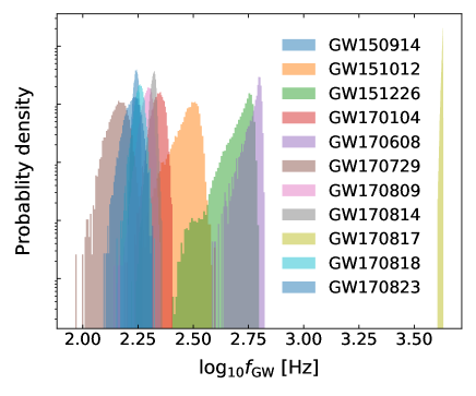
Figure 2: Probability density for $f_{\rm GW}$, generated using the posterior samples provided by the LIGO/Virgo Collaboration Abbott et al. (2019a); GWT (a, b) and the fit in Eq. (18) Bohé et al. (2017).

In order to construct the gLIV tests with Eq. (11) in practice, we make the following considerations.

1. For the same reason as that in the photon sector Kostelecký and Mewes (2002, 2009); Shao and Ma (2011), in these propagation tests vacuum birefringent phenomena can constrain gLIV parameters more tightly than the dispersive ones. Because $\zeta^{0}_{(d)}$, so as $\tilde{\zeta}^{0}_{(d)}$, introduces polarization-independent time delays, they are comparably loosely bound. Nevertheless, if GW companion particles (photons or neutrinos) are detected, the dispersion can be fairly constrained; for example, see the bound on the SME $\bar{s}_{00}^{(4)}$ parameter via the simultaneous observation of GW170817 and GRB 170817A Abbott et al. (2017c). To bound the scope of this paper with fair workload, these polarization-independent, dispersive-only delays, encoded in $\zeta^{0}_{(d)}$ and $\tilde{\zeta}^{0}_{(d)}$, are omitted in the following analysis. They can be incorporated in future work.

2. For the GW frequency at the amplitude peak, we use the dedicated fit for the $(2,2)$ mode in the Appendix A.3 of Ref. Bohé et al. (2017). The fit was obtained by combining catalogs of numerical relativity Boyle et al. (2019) and test-particle Teukolsky-code waveforms. It includes the contribution from the mass ratio of the binary and the orbit-aligned spins of the binary components. The fit is adopted in the so-called SEOBNRv4 waveform family Bohé et al. (2017), and is being extensively applied in the LIGO/Virgo daily data analysis. An explicit expression for the global fit is given in Appendix C and several examples for different spin combinations are given in Fig. 6 therein. Different waveform families give very close, practically indistinguishable results Abbott et al. (2017d). Using the posterior samples provided by the LIGO/Virgo Collaboration Abbott et al. (2019a); GWT (a, b), we plot the GW peak frequencies for the 11 GW events in Fig. 2. Notice that, while the fit was obtained from BBH simulations without matter effects, its prediction to the BNS event GW170817, whose nuclear matter effects enter the waveform at the fifth post-Newtonian order Hinderer and Flanagan (2008); Abbott et al. (2019d), should be indicative for the analysis in this work. Because the merger part for BNS was not actually observed in GW detectors Abbott et al. (2017b, 2019d), in our tests we conservatively use a rather arbitrary value $f_{\rm GW}=800$ Hz for GW170817. It roughly corresponds to the cutoff sensitivity at high-frequency end for LIGO/Virgo detectors at the time of GW170817. Larger values of $f_{\rm GW}$ would lead to tighter constraints.

3. For the time delay between two circularly polarized GW modes, we use a simple order-of-magnitude estimation, $\left|\omega_{\rm GW}\Delta t\right|\leq 2\pi/\rho$, where $\Delta t$ is the time difference between two circular modes, and $\rho$ is the network signal-to-noise ratio (SNR) of the observed GW events (see Table 6 in Appendix A). We expect this estimation to work fairly well at the current stage in constraining the gLIV phenomena, instead of discovering the gLIV phenomena. One direction to improve the investigation would be using the matched-filtering technique with modified/deformed gravitational waveforms Mewes (2019). For such an improved study, our results from individual events can be rescaled accordingly. Study along this line can be used to verify our assumption. For now we leave a dedicated analysis to future work.

4. Limited by the number of available GW events we will focus on (i) the mass dimension $d=5$ gLIV coefficients $k^{(5)}_{(V)jm}$, and (ii) the mass dimension $d=6$ gLIV coefficients $k^{(6)}_{(E)jm}$ and $k^{(6)}_{(B)jm}$. As mentioned before, mathematically it is required that $|s|\leq j\leq d-2$; therefore, when $d=5$, $j=0,1,2,3$ for $k^{(5)}_{(V)jm}$, and when $d=6$, $j$ only takes the value $4$ for $k^{(6)}_{(E)jm}$ and $k^{(6)}_{(B)jm}$. In general, the components of $\left\{k^{(d)}_{(V)jm},k^{(d)}_{(E)jm},k^{(d)}_{(B)jm}\right\}$ are complex numbers, satisfying $\left(k_{jm}^{(d)}\right)^{*}=(-1)^{m}k_{j(-m)}^{(d)}$ Mewes (2019). Thus, we will deal with in total, (i) $(d-1)^{2}=16$ independent components for $k^{(5)}_{(V)jm}$, and (ii) $(d-1)^{2}-16=9$ independent components for $k^{(6)}_{(E)jm}$ and $k^{(6)}_{(B)jm}$ each.

In a short summary, on one hand we have 11 two-sided constraints from 11 GW events in the GWTC-1, and on the other hand, we need to constrain $16$ independent components when $d=5$, and $9+9=18$ independent components when $d=6$. Therefore, it is an over-constraining system. The reason for the GW propagation constraints being “two sided” is that, we do not expect either circular mode travels faster than the other one; otherwise, the deformation in the waveforms would be quite obvious Mewes (2019).

Table 2: The maximal-reach 1-$\sigma$ limits on the magnitude of $k^{(5)}_{(V)jm}$ by assuming that the other gLIV coefficients are zero. The tightest constraints from an individual GW event are listed alongside with the event names. The combined constraints are obtained via $\sigma^{\rm(combined)}\equiv 1/\sqrt{\sum_{i}^{N_{\rm GW}}1/\sigma_{i}^{2}}$. All limits are given in unit of $10^{-16}\,{\rm m}$.

$j$	$m$	Component	Individual	GW	Combined
0	0	$\left|k^{(5)}_{(V)00}\right|$	$5.3$	GW170608	3.3
1	0	$\left|k^{(5)}_{(V)10}\right|$	$3.5$	GW170608	2.7
1	1	$\left|{\rm Re}\,k^{(5)}_{(V)11}\right|$	$8.9$	GW151226	4.7
		$\left|{\rm Im}\,k^{(5)}_{(V)11}\right|$	$8.9$	GW151226	4.7
2	0	$\left|k^{(5)}_{(V)20}\right|$	$3.8$	GW170608	3.1
2	1	$\left|{\rm Re}\,k^{(5)}_{(V)21}\right|$	$4.9$	GW170608	3.4
		$\left|{\rm Im}\,k^{(5)}_{(V)21}\right|$	$4.9$	GW170608	3.4
2	2	$\left|{\rm Re}\,k^{(5)}_{(V)22}\right|$	$8.6$	GW170817	5.8
		$\left|{\rm Im}\,k^{(5)}_{(V)22}\right|$	$8.6$	GW170817	5.8
3	0	$\left|k^{(5)}_{(V)30}\right|$	$6.8$	GW151226	3.9
3	1	$\left|{\rm Re}\,k^{(5)}_{(V)31}\right|$	$3.7$	GW170608	3.1
		$\left|{\rm Im}\,k^{(5)}_{(V)31}\right|$	$3.7$	GW170608	3.1
3	2	$\left|{\rm Re}\,k^{(5)}_{(V)32}\right|$	$7.8$	GW170608	4.4
		$\left|{\rm Im}\,k^{(5)}_{(V)32}\right|$	$7.8$	GW170608	4.4
3	3	$\left|{\rm Re}\,k^{(5)}_{(V)33}\right|$	$8.3$	GW170817	6.5
		$\left|{\rm Im}\,k^{(5)}_{(V)33}\right|$	$8.3$	GW170817	6.5

Table 3: Same as Table 2, for $k^{(6)}_{(E)jm}$ and $k^{(6)}_{(B)jm}$. All limits are given in unit of $10^{-11}\,{\rm m}^{2}$.

$j$	$m$	Component	Individual	GW	Combined
4	0	$\left|k^{(6)}_{(E,B)40}\right|$	$4.9$	GW170817	4.8
4	1	$\left|{\rm Re}\,k^{(6)}_{(E,B)41}\right|$	$5.0$	GW170817	4.6
		$\left|{\rm Im}\,k^{(6)}_{(E,B)41}\right|$	$5.0$	GW170817	4.6
4	2	$\left|{\rm Re}\,k^{(6)}_{(E,B)42}\right|$	$5.7$	GW170817	4.1
		$\left|{\rm Im}\,k^{(6)}_{(E,B)42}\right|$	$5.7$	GW170817	4.1
4	3	$\left|{\rm Re}\,k^{(6)}_{(E,B)43}\right|$	$3.9$	GW170608	3.0
		$\left|{\rm Im}\,k^{(6)}_{(E,B)43}\right|$	$3.9$	GW170608	3.0
4	4	$\left|{\rm Re}\,k^{(6)}_{(E,B)44}\right|$	$2.7$	GW170608	2.4
		$\left|{\rm Im}\,k^{(6)}_{(E,B)44}\right|$	$2.7$	GW170608	2.4

IV Numerical resutls

With all the practical considerations in Secs. II and III taken into account, we present our final numerical constraints on the gLIV coefficients in this section. As mentioned above, it is an over-constraining system. Therefore, we can consequently bound globally all independent coefficients at a specific mass dimension $d$ using the whole GW catalog. However, we will first consider the maximal-reach scenario Tasson (2019); Kostelecký and Russell (2011) where only one independent component is assumed to be nonzero. It eases comparison with results in Ref. Kostelecký and Mewes (2016), and provides us some insight on the figure of merit for different GW events in testing the anisotropic birefringence.

Because the GW parameters are generally highly correlated, we use the posterior samples provided by the LIGO/Virgo Collaboration GWT (a, b) which include all correlations among parameters and are publicly available. For the ten BBHs, we use the posterior samples tagged with Overall_posterior that are combined results derived from the effective-one-body and phenomenological waveform families Abbott et al. (2019a), while for the BNS GW170817, we use the samples tagged with IMRPhenomPv2NRT_lowSpin_posterior that are derived from an effectively-precessing phenomenological waveform family with the tidal deformability effects incorporated Abbott et al. (2019d). Other choices do not change our limits in a significant way. The GW parameters we use include, (i) the sky position represented by the right ascension, $\alpha$, and the declination, $\delta$ (see Fig. 5 in Appendix A); (ii) the intrinsic GW parameters including the component masses, $m_{1}$ and $m_{2}$, and the (dimensionless) orbital-aligned component spins, $\chi_{1}$ and $\chi_{2}$; and (iii) the luminosity distance $d_{L}$ from where the redshift, and then the $D_{\alpha}^{(d)}$ in Eq. (12), are derived with the standard $\Lambda$CDM model Aghanim et al. (2018).

In the maximal-reach scenario, we assume that only one gLIV parameter is nonzero at a time Tasson (2019). For each GW event, we randomly draw samples from the posteriors. We calculate the individual limit for each gLIV parameter for each sample point. The results are stored for statistical inference afterwards. After accumulating enough samples, the 1-$\sigma$ limits are obtained from their corresponding distributions. In the calculation, all statistical uncertainties are taken into account properly.

In Tables 2 and 3, respectively for mass dimensions $d=5$ and $d=6$, we list the maximal-reach limits for each gLIV component. We have put the tightest limit from an individual GW event, along with the event name in the fourth and fifth columns. We can see that, for mass dimension-5 operators, the individually tightest limits come from GW151226, GW170608, and GW170817, while for mass dimension-6 operators, the individually tightest limits come from GW170608 and GW170817. These events all have low component masses.

Usually, low-mass events are detected closer to the Earth, because their GW strain amplitudes are smaller than high-mass ones if they were put at a same distance Maggiore (2007); Abbott et al. (2018). The finite sensitivity of GW detectors can only pick up those low-mass events relatively nearby Abbott et al. (2018). For the three individually best events here (GW151226, GW170608, and GW170817), they all have the cosmological redshift $z\lesssim 0.1$ (see Table 6). Although the GW propagation tests benefit from large distances [see Eq. (12)], which usually correspond to high-mass GW events (see Table 6), our anisotropic birefringent tests also depend on the GW frequency with a powerlaw index $d-4$ [see Eq. (11)], which is positive for $d=5$ and $6$. High-mass GW events have a lower GW frequency [see Eq. (18)] Maggiore (2007), which decreases their ability to constrain the gLIV parameters. Our results clearly show that, already at mass dimension 5, low-mass events are preferred to the tests of the gLIV parameters in the SME. At mass dimension 6, the benefit from smaller masses is even more prominent. The dependence of the bounds on other parameters, e.g. the precision of sky localization, deserves further study.

For the maximal-reach scenario, we also list the combined limits from multiple GWs by assuming each event mutually independently. Therefore, one gets a combined limit $\sigma^{\rm(combined)}\simeq 1/\sqrt{\sum_{i}^{N_{\rm GW}}1/\sigma_{i}^{2}}$, where $\sigma_{i}$ is the limit from an individual GW event $i$. As we can see, the combined limit improves the limit from the individually best event by a factor smaller than two. Therefore, in the maximal-reach approach, the limit is dominated by the individually best GW event. Worth to mention that, the limits in Tables 2 and 3 improve over the first set of limits from GW150914 Kostelecký and Mewes (2016) by a factor $\sim 10^{2}$–$10^{4}$ for the mass dimension $d=5$, and by a factor $\sim 10^{3}$–$10^{5}$ for the mass dimension $d=6$.

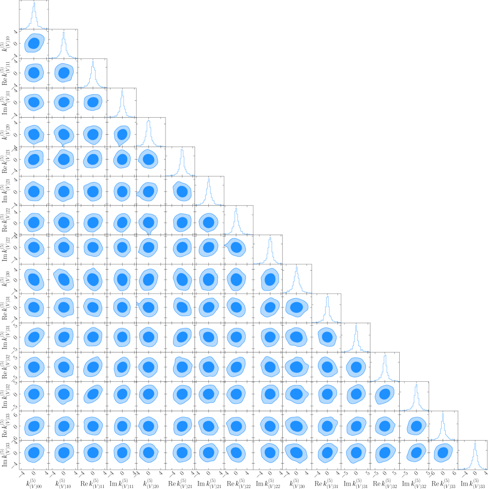
Figure 3: Global constraints on 16 independent gLIV components with mass dimension $d=5$ from 11 GW events in the GWTC-1. Contours show the 68% and 90% confidence levels. The unit for the limits is $10^{-15}\,{\rm m}$ in this figure.

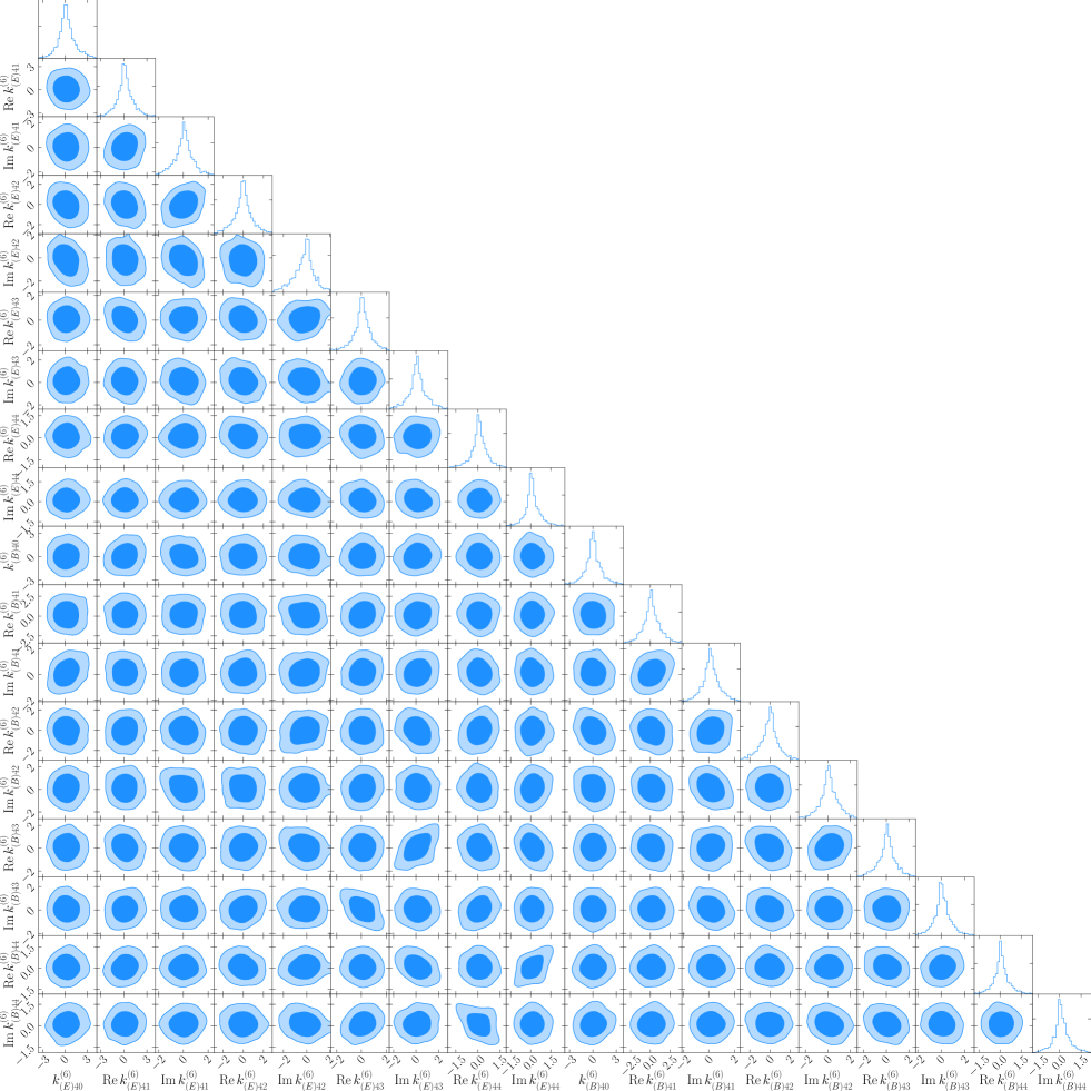
Figure 4: Same as Fig. 3, for the 18 independent gLIV components with mass dimension $d=6$. The unit for the limits is $10^{-10}\,{\rm m}^{2}$ in this figure.

The maximal-reach limits should be considered as quite optimistic, and in reality they should be bounds on some linear combinations of the underlying set of gLIV coefficients Kostelecký and Mewes (2016). Therefore, it becomes very intriguing to break the degeneracy among these parameters and check the real power of GW events in probing the gLIV when a number of events are available Kostelecký and Russell (2011). In the following, we use the simple facts, that (i) different GW events come from different directions Abbott et al. (2019a) and (ii) symmetry breaking in the SME is observer Lorentz-invariant Bluhm and Kostelecký (2005), to globally constrain these gLIV parameters. This is possible, because the coefficients of the linear combinations are direction-dependent, depending on the direction $\hat{\bm{n}}$ via the spin-weighted spherical harmonics functions; see Eqs. (7–9) and Appendix B.

Table 4: Global constraints on $k^{(5)}_{(V)jm}$ at the 68% confidence level. Notice that the unit differs from that in Table 2.

$j$	$m$	Component	Constraint [$10^{-15}\,{\rm m}$]
0	0	$k^{(5)}_{(V)00}$	$(-0.94,0.96)$
1	0	$k^{(5)}_{(V)10}$	$(-1.01,1.03)$
1	1	${\rm Re}\,k^{(5)}_{(V)11}$	$(-0.99,1.06)$
		${\rm Im}\,k^{(5)}_{(V)11}$	$(-0.89,0.84)$
2	0	$k^{(5)}_{(V)20}$	$(-1.00,0.94)$
2	1	${\rm Re}\,k^{(5)}_{(V)21}$	$(-1.12,1.08)$
		${\rm Im}\,k^{(5)}_{(V)21}$	$(-0.96,1.00)$
2	2	${\rm Re}\,k^{(5)}_{(V)22}$	$(-0.97,1.19)$
		${\rm Im}\,k^{(5)}_{(V)22}$	$(-1.13,0.93)$
3	0	$k^{(5)}_{(V)30}$	$(-1.38,1.43)$
3	1	${\rm Re}\,k^{(5)}_{(V)31}$	$(-1.13,0.98)$
		${\rm Im}\,k^{(5)}_{(V)31}$	$(-1.26,1.25)$
3	2	${\rm Re}\,k^{(5)}_{(V)32}$	$(-1.54,1.46)$
		${\rm Im}\,k^{(5)}_{(V)32}$	$(-1.22,1.14)$
3	3	${\rm Re}\,k^{(5)}_{(V)33}$	$(-1.45,1.50)$
		${\rm Im}\,k^{(5)}_{(V)33}$	$(-1.20,0.98)$

Table 5: Same as Table 4, for $k^{(6)}_{(E)jm}$ and $k^{(6)}_{(B)jm}$.

$j$	$m$	Component	Constraint [$10^{-10}\,{\rm m}^{2}$]
4	0	$k^{(6)}_{(E)40}$	$(-0.76,1.32)$
4	1	${\rm Re}\,k^{(6)}_{(E)41}$	$(-0.81,1.16)$
		${\rm Im}\,k^{(6)}_{(E)41}$	$(-0.68,0.72)$
4	2	${\rm Re}\,k^{(6)}_{(E)42}$	$(-0.85,0.81)$
		${\rm Im}\,k^{(6)}_{(E)42}$	$(-1.11,0.55)$
4	3	${\rm Re}\,k^{(6)}_{(E)43}$	$(-0.57,0.69)$
		${\rm Im}\,k^{(6)}_{(E)43}$	$(-0.58,0.88)$
4	4	${\rm Re}\,k^{(6)}_{(E)44}$	$(-0.39,0.58)$
		${\rm Im}\,k^{(6)}_{(E)44}$	$(-0.32,0.67)$
4	0	$k^{(6)}_{(B)40}$	$(-0.87,1.02)$
4	1	${\rm Re}\,k^{(6)}_{(B)41}$	$(-0.82,1.21)$
		${\rm Im}\,k^{(6)}_{(B)41}$	$(-0.47,0.80)$
4	2	${\rm Re}\,k^{(6)}_{(B)42}$	$(-0.93,0.74)$
		${\rm Im}\,k^{(6)}_{(B)42}$	$(-0.63,0.87)$
4	3	${\rm Re}\,k^{(6)}_{(B)43}$	$(-0.70,0.76)$
		${\rm Im}\,k^{(6)}_{(B)43}$	$(-0.55,0.77)$
4	4	${\rm Re}\,k^{(6)}_{(B)44}$	$(-0.39,0.60)$
		${\rm Im}\,k^{(6)}_{(B)44}$	$(-0.34,0.64)$

We have two sets of global analysis, for mass dimension $5$ and mass dimension $6$. In each global analysis, we assume that all anisotropic-birefringent gLIV coefficients can be nonzero at that specific $d$. Therefore, we have in total 16 independent coefficients for $d=5$, and 18 independent coefficients for $d=6$. Fortunately, the 11 events in GWTC-1 provide us in total 22 useful constraints.

The global analysis for $d=5$ is relatively easier, because (i) the square root in Eq. (11) is plainly calculated when $\tilde{\zeta}_{(d=5)}^{1}=\tilde{\zeta}_{(d=5)}^{2}=0$, and (ii) only the $s=0$ spherical harmonics are involved. Similarly to the maximal-reach case, we randomly draw posterior samples, but now simultaneously for 11 events. Their time delays are drawn from zero-mean Gaussian distributions with their standard variances determined in Sec. III. Then, for each random draw, we construct the global likelihood as a function of the 16 gLIV coefficients. The likelihood is maximized by the routines in the Scipy.Optimize package Virtanen et al. (2020). Thus, values of 16 coefficients are calculated in each random draw. The resulted values for the 16 gLIV coefficients are recorded for later inference. After we accumulate enough draws, we extract the constraints on the 16 gLIV coefficients from these recorded distributions.

The 1-dimensional marginalized constraints are listed in Table 4, and the contour plots for these parameters are given in Fig. 3. It is interesting to note that, (i) the global constraints are only about a factor of $10$ weaker than the maximal-reach limits, and (ii) these 16 gLIV parameters are hardly correlated. The small correlation between parameters is resulted from the use of multiple events. It shows the advantage of constructing an over-constraining system with multiple events, analogous to the cases of using millisecond pulsars under a similar context Shao (2014a); Shao and Bailey (2018, 2019).

The global analysis for $d=6$ is somehow complicated. Now we have the spin-weighted spherical harmonics with $s=\pm 4$. To reduce the computational cost, we use ${}_{s}Y_{jm}^{*}={(-1)^{s+m}}\,{{}_{-s}Y_{j(-m)}}$ to calculate ${{}_{-4}Y_{jm}}$ from ${{}_{+4}Y_{jm}}$. More importantly, in the most general case for $d=6$, we have $\tilde{\zeta}_{(d=6)}^{1}\neq 0$ and $\tilde{\zeta}_{(d=6)}^{2}\neq 0$. As a consequence, the square root in Eq. (11) is nontrivial. Therefore, the calculation with these highly nonlinear features takes a much longer computer time, namely, the Scipy.Optimize routines now need much more significant computational time to iterate, in order to locate the maximum of the 18-dimensional likelihood functions. Nevertheless, the principles are similar to the $d=5$ case. The results for $d=6$ are give in Table 5 and Fig. 4. Similar conclusions that were made for $d=5$ operators in the last paragraph can be made for $d=6$ operators as well.

V Discussion

Gravitational Lorentz invariance violation (gLIV) is a central topic in the program of using the gravitational waves (GWs) to probe the most fundamental principles in modern physics Abbott et al. (2017a, 2019b); Kostelecký and Mewes (2016); Nishizawa (2018); Yunes et al. (2016); Berti et al. (2018a, b). If the Lorentz symmetry is broken in the gravity sector, there might be a preferred frame Will (2014, 2018) where the breaking is isotropic, but a more generic breaking does not need a preferred frame Kostelecký (2004); Bailey and Kostelecký (2006). Isotropic gLIV, being a specific class of gLIV, was studied in details Mirshekari et al. (2012); Abbott et al. (2017a, 2019b); Wang and Zhao (2020); Nishizawa (2018). Most of previous work focused on non-birefringent phenomena in searches of the gLIV. Extensions to these studies are needed. On one hand, because the commutator of two boost generators is a generator for rotation, anisotropy is inevitable in a complete search for the gLIV. On the other hand, in effective field theories, the most general gLIV has birefringent behaviors for the two circularly polarized GW eigen-modes in the nonminimal gravity. In this work, we take a leap to systematically study anisotropic birefringent phenomena related to the GW propagation with the GW transient catalog GWTC-1 Abbott et al. (2019a); GWT (a, b).

One of the best theoretical frameworks, in carrying out these anisotropic birefringent gLIV tests, is the standard-model extension (SME) Kostelecký (2004); Kostelecký and Mewes (2016); Mewes (2019). We follow the spirit of effective field theories, and assume that the gLIV happens at a specific mass dimension $d$. The lowest mass dimensions for vacuum birefringence are $d=5$ and $d=6$. When $d=5$, there are in total 16 independent gLIV coefficients in $k_{(V)jm}^{(5)}$, while $d=6$, there are 18 independent gLIV coefficients in $k_{(E)jm}^{(6)}$ and $k_{(B)jm}^{(6)}$. In our global tests, we simultaneously include all gLIV operators that lead to birefringence at that particular mass dimension. We use the posterior samples for the events in GWTC-1, provided by the LIGO/Virgo Collaboration, to coherently solve for gLIV parameters, and obtain their constraints thereof. Our maximal-reach limits are listed in Tables 2 and 3, and our global limits are presented in Tables 4 and 5, as well as in Figs. 3 and 4. No violation of Einstein’s general relativity was found, and the constraints on 34 gLIV coefficients are improved by factors ranging from $\sim 10^{2}$ to $\sim 10^{5}$, with respect to previous limits Kostelecký and Mewes (2016).

The gLIV tests can be improved in multiple directions in the future. (I) A more sophisticated matched-filtering analysis with gLIV-deformed waveforms Mewes (2019) can be used to validate the assumptions made in this work, though such an analysis could have cost mighty computational time in practice for a catalog of GWs. (II) Another possibility in testing the GW propagation can involve modified cosmological behaviors. For example, Nishizawa (2018) considered a generic GW propagation equation,

$$h_{ij}^{\prime\prime}+\left(2+\nu\right){\cal H}h_{ij}^{\prime}+\left(c_{T}^{2}k^{2}+a^{2}\mu^{2}\right)h_{ij} =a^{2}\Gamma\gamma_{ij}\,,$$ (15)

which — besides the cosmological expansion encoded in ${\cal H}\equiv a^{\prime}/a$ with $a$ being the cosmological scale factor — includes running of the Planck mass $M_{*}$ via $\nu={\cal H}^{-1}d\ln M_{*}^{2}/dt$, the velocity of GWs $c_{T}$, the mass of graviton $\mu$, and the anisotropic source term $\Gamma\gamma_{ij}$. The philosophy of the approach (15) is different from ours which is based on a modified action of the gravity sector [see Eq. (2)]. Nevertheless, a grander theoretical framework that includes both a modified-gravity action and a modified cosmology might be feasible. It lays beyond the scope of this work however. (III) The final obvious direction to improve the tests in this work is to involve more GW events. Actually, more and yet more accurately-measured GW events are undoubtfully expected Abbott et al. (2018). With the ongoing third observing run by the LIGO/Virgo Collaboration, more GW event candidates are already revealed for possible electromagnetic followups O3: . At the time of writing, a second BNS, GW190425, was published Abbott et al. (2020). This event is weaker than GW170817, but it will help in constraining the gLIV parameters in the global analysis. With the KAGRA Aso et al. (2013) and IndiGO GW detectors coming online in the near future, even better limits will be placed on the gLIV. Ultimately, we hope some positive clues to the long-sought quantum gravity theory might be uncovered via GWs.

Table 6: Source parameters for 11 confident detections in the GWTC-1, from the first and second LIGO/Virgo observing runs Abbott et al. (2019a). Uncertainties are from the symmetric 90% credible intervals. For the network SNR, we list the average from three detection pipelines (PyCBC, GstLAL, cWB; see Ref. Abbott et al. (2019a) for details).

	Type	$m_{1}~{}[M_{\odot}]$	$m_{2}~{}[M_{\odot}]$	$d_{L}~{}[{\rm Mpc}]$	Redshift $z$	Localization $\Delta\Omega~{}[{\rm deg}^{2}]$	Network SNR
GW150914	BBH	$35.6^{+4.8}_{-3.0}$	$30.6^{+3.0}_{-4.4}$	$430^{+150}_{-170}$	$0.09^{+0.03}_{-0.03}$	180	24.4
GW151012	BBH	$23.3^{+14.0}_{-5.5}$	$13.6^{+4.1}_{-4.8}$	$1060^{+540}_{-480}$	$0.21^{+0.09}_{-0.09}$	$1555$	9.8
GW151226	BBH	$13.7^{+8.8}_{-3.2}$	$7.7^{+2.2}_{-2.6}$	$440^{+180}_{-190}$	$0.09^{+0.04}_{-0.04}$	1033	12.7
GW170104	BBH	$31.0^{+7.2}_{-5.6}$	$20.1^{+4.9}_{-4.5}$	$960^{+430}_{-410}$	$0.19^{+0.07}_{-0.08}$	924	13.0
GW170608	BBH	$10.9^{+5.3}_{-1.7}$	$7.6^{+1.3}_{-2.1}$	$320^{+120}_{-110}$	$0.07^{+0.02}_{-0.02}$	396	14.8
GW170729	BBH	$50.6^{+16.6}_{-10.2}$	$34.3^{+9.1}_{-10.1}$	$2750^{+1350}_{-1320}$	$0.48^{+0.19}_{-0.20}$	1033	10.3
GW170809	BBH	$35.2^{+8.3}_{-6.0}$	$23.8^{+5.2}_{-5.1}$	$990^{+320}_{-380}$	$0.20^{+0.05}_{-0.07}$	340	12.3
GW170814	BBH	$30.7^{+5.7}_{-3.0}$	$25.3^{+2.9}_{-4.1}$	$580^{+160}_{-210}$	$0.12^{+0.03}_{-0.04}$	87	16.5
GW170817	BNS	$1.46^{+0.12}_{-0.10}$	$1.27^{+0.09}_{-0.09}$	$40^{+10}_{-10}$	$0.01^{+0.00}_{-0.00}$	16	32.0
GW170818	BBH	$35.5^{+7.5}_{-4.7}$	$26.8^{+4.3}_{-5.2}$	$1020^{+430}_{-360}$	$0.20^{+0.07}_{-0.07}$	39	11.3
GW170823	BBH	$39.6^{+10.0}_{-6.6}$	$29.4^{+6.3}_{-7.1}$	$1850^{+840}_{-840}$	$0.34^{+0.13}_{-0.14}$	1651	11.1

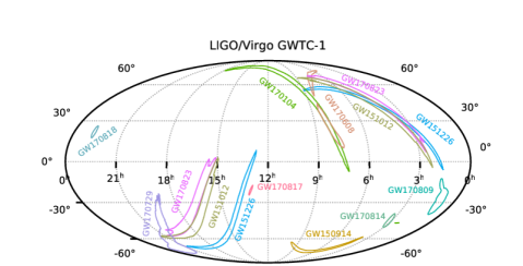
Figure 5: Sky localization of GW events in the GWTC-1 catalog from LIGO/Virgo’s first and second observing runs, at the 68% confidence level Abbott et al. (2019a).

Appendix A A brief summary of GWTC-1

In the Advanced LIGO/Virgo’s first and second observing runs, respectively taking place from September 12, 2015 to January 19, 2016, and from November 30, 2016 to August 25, 2017, ten confident detections of BBHs and one confident detection of BNSs were reported Abbott et al. (2019a). In Table 6, we list the basic parameters and their uncertainties for these events Abbott et al. (2019a). As sky position is important in testing anisotropic birefringence, in Fig. 5 we show the 68% credible regions for sky location of GW events in the GWTC-1 Abbott et al. (2019a), in a Mollweide projection in the equatorial coordinate. Data are taken from the associated data release for the sky maps GWT (c) to the LIGO/Virgo’s GWTC-1 GWT (a), hosted by the Gravitational Wave Open Science Center (GWOSC) GWS . The plot has made use of the ligo.skymap package pac , maintained by Leo Singer.

In all of the numerical calculations of this paper, we have used the posterior samples provided by the LIGO/Virgo Collaboration, hosted at the GWOSC GWT (b).

Notice that the uncertainties are rather heterogeneous for different GW events, due to the operation of GW detectors in practice at the detection time. In particular, the sky localization plays an essential role in determining the anisotropic behavior of gLIV, which should be taken into full account, as is done in this work.

Appendix B Spin-weighted spherical harmonics

As we are familiar with the ordinary spherical harmonics, $Y_{jm}\equiv{{}_{0}Y_{jm}}$, in describing scalars’ irreducible decomposition in three dimensions, the spin-weighted spherical harmonics, ${}_{s}Y_{jm}$, are widely used to decompose other tensors with definite orbital and spin angular momentum Newman and Penrose (1966); Goldberg et al. (1967).

While mathematical and physical discussions can be found respectively in Refs. Newman and Penrose (1966); Goldberg et al. (1967) and in the Appendix A of Ref. Kostelecký and Mewes (2009), here in our calculation we use the explicit expression of ${}_{s}Y_{jm}$ in a brute-force manner. It reads Newman and Penrose (1966); Goldberg et al. (1967); Kostelecký and Mewes (2009),

$${}_{s}Y_{jm}(\theta,\phi)= \sqrt{\frac{2j+1}{4\pi}\frac{(j+m)!(j-m)!}{(j+s)!(j-s)!}}e^{im\phi}\left(\sin\frac{\theta}{2}\right)^{2j}$$

$$\sum_{r}(-1)^{j+m+s+r}C^{r}_{j-s}C_{j+s}^{r+s-m}\left(\cot\frac{\theta}{2}\right)^{2r+s-m}\,,$$ (16)

where $C_{n}^{k}$ denotes the binomial coefficients. Interested readers are referred to the above references for topics related to raising and lowering operators, orthogonality relation, completeness relation, physical interpretation with respect to the angular momentum, etc..

Appendix C Global fit to GW frequency at the merger

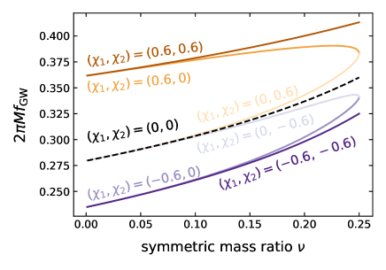
Figure 6: Examples of the GW peak frequency as a function of the symmetric mass ratio $\nu$, for several orbit-aligned spin combinations.

To obtain an accurate estimation of GW frequency at the merger of a binary system of masses $m_{1}$ and $m_{2}$ (assuming $m_{1}\geq m_{2}$) and (orbit-aligned) dimensionless spins $\chi_{1}$ and $\chi_{2}$, we adopt the global fit in the Appendix A.3 of Ref. Bohé et al. (2017). It bases on catalogs of waveforms from numerical relativity Boyle et al. (2019) and test-particle Teukolsky code. Consider a binary with a symmetric mass ratio $\nu\equiv m_{1}m_{2}/M^{2}$ where $M\equiv m_{1}+m_{2}$, and an effective spin variable,

$$\chi\equiv\chi_{\mathrm{S}}+\frac{\chi_{\mathrm{A}}}{1-2\nu}\delta\,,$$ (17)

where $\chi_{\mathrm{S},\mathrm{A}}\equiv\left(\chi_{1}\pm\chi_{2}\right)/2$, and $\delta\equiv\left(m_{1}-m_{2}\right)/M$. The global fit for the dominant $(2,2)$ mode has the form Bohé et al. (2017),

$$2\pi Mf_{\rm GW}\left(\nu,\chi\right)=p_{0}+\left(p_{1}+p_{2}\chi\right)\log\left({\cal A}-{\cal B}\chi\right)\,,$$ (18)

where

$${\cal A} =p_{3}+4\left(p_{3}-p_{4}\right)\left(\nu-\frac{1}{4}\right)\,,$$ (19)

$${\cal B} =p_{5}+4\left(p_{5}-p_{6}\right)\left(\nu-\frac{1}{4}\right)\,,$$ (20)

and

$$p_{0} =0.562679\,,$$

$$p_{1} =-0.087062\,, p_{2} =0.001743\,,$$

$$p_{3} =10.262073\,, p_{4} =25.850378\,,$$

$$p_{5} =7.629922\,, p_{6} =25.819795\,.$$

In Fig. 6 we show examples of the GW peak frequency for several combinations of the orbit-aligned spins, as a function of $\nu$. In our tests of gLIV in the main text, we have used the posteriors of component masses and orbital-aligned component spins to infer $f_{\rm GW}$.

References

- Jacobson et al. (2006) T. Jacobson, S. Liberati, and D. Mattingly, Annals Phys. 321, 150 (2006), arXiv:astro-ph/0505267 [astro-ph] .
- Tasson (2014) J. D. Tasson, Rept. Prog. Phys. 77, 062901 (2014), arXiv:1403.7785 [hep-ph] .
- Kostelecký and Samuel (1989) V. A. Kostelecký and S. Samuel, Phys. Rev. D 39, 683 (1989).
- Kostelecký and Potting (1991) V. A. Kostelecký and R. Potting, Nucl. Phys. B 359, 545 (1991).
- Mattingly (2005) D. Mattingly, Living Rev. Rel. 8, 5 (2005), arXiv:gr-qc/0502097 [gr-qc] .
- Kostelecký and Russell (2011) V. A. Kostelecký and N. Russell, Rev. Mod. Phys. 83, 11 (2011), arXiv:0801.0287 [hep-ph] .
- Carroll et al. (1990) S. M. Carroll, G. B. Field, and R. Jackiw, Phys. Rev. D 41, 1231 (1990).
- Colladay and Kostelecký (1997) D. Colladay and V. A. Kostelecký, Phys. Rev. D 55, 6760 (1997), arXiv:hep-ph/9703464 [hep-ph] .
- Colladay and Kostelecký (1998) D. Colladay and V. A. Kostelecký, Phys. Rev. D 58, 116002 (1998), arXiv:hep-ph/9809521 [hep-ph] .
- Kostelecký (2004) V. A. Kostelecký, Phys. Rev. D 69, 105009 (2004), arXiv:hep-th/0312310 [hep-th] .
- Hees et al. (2016) A. Hees, Q. G. Bailey, A. Bourgoin, H. P.-L. Bars, C. Guerlin, and C. Le Poncin-Lafitte, Universe 2, 30 (2016), arXiv:1610.04682 [gr-qc] .
- Shao and Wex (2016) L. Shao and N. Wex, Sci. China Phys. Mech. Astron. 59, 699501 (2016), arXiv:1604.03662 [gr-qc] .
- Tasson (2016) J. D. Tasson, Symmetry 8, 111 (2016), arXiv:1610.05357 [gr-qc] .
- Will (2014) C. M. Will, Living Rev. Rel. 17, 4 (2014), arXiv:1403.7377 [gr-qc] .
- Berti et al. (2015) E. Berti et al., Class. Quant. Grav. 32, 243001 (2015), arXiv:1501.07274 [gr-qc] .
- Amelino-Camelia et al. (1998) G. Amelino-Camelia, J. R. Ellis, N. E. Mavromatos, D. V. Nanopoulos, and S. Sarkar, Nature 393, 763 (1998), arXiv:astro-ph/9712103 [astro-ph] .
- Gambini and Pullin (1999) R. Gambini and J. Pullin, Phys. Rev. D 59, 124021 (1999), arXiv:gr-qc/9809038 [gr-qc] .
- Amelino-Camelia (2013) G. Amelino-Camelia, Living Rev. Rel. 16, 5 (2013), arXiv:0806.0339 [gr-qc] .
- Will (2018) C. M. Will, Theory and Experiment in Gravitational Physics (Cambridge University Press, 2018).
- Kostelecký and Tasson (2011) V. A. Kostelecký and J. D. Tasson, Phys. Rev. D 83, 016013 (2011), arXiv:1006.4106 [gr-qc] .
- Bluhm and Kostelecký (2005) R. Bluhm and V. A. Kostelecký, Phys. Rev. D 71, 065008 (2005), arXiv:hep-th/0412320 [hep-th] .
- Battat et al. (2007) J. B. R. Battat, J. F. Chandler, and C. W. Stubbs, Phys. Rev. Lett. 99, 241103 (2007), arXiv:0710.0702 [gr-qc] .
- Bourgoin et al. (2017) A. Bourgoin, C. Le Poncin-Lafitte, A. Hees, S. Bouquillon, G. Francou, and M.-C. Angonin, Phys. Rev. Lett. 119, 201102 (2017), arXiv:1706.06294 [gr-qc] .
- Mueller et al. (2008) H. Mueller, S.-w. Chiow, S. Herrmann, S. Chu, and K.-Y. Chung, Phys. Rev. Lett. 100, 031101 (2008), arXiv:0710.3768 [gr-qc] .
- Kostelecký and Tasson (2015) V. A. Kostelecký and J. D. Tasson, Phys. Lett. B 749, 551 (2015), arXiv:1508.07007 [gr-qc] .
- Shao (2014a) L. Shao, Phys. Rev. Lett. 112, 111103 (2014a), arXiv:1402.6452 [gr-qc] .
- Shao (2014b) L. Shao, Phys. Rev. D 90, 122009 (2014b), arXiv:1412.2320 [gr-qc] .
- Jennings et al. (2015) R. J. Jennings, J. D. Tasson, and S. Yang, Phys. Rev. D 92, 125028 (2015), arXiv:1510.03798 [gr-qc] .
- Shao and Bailey (2018) L. Shao and Q. G. Bailey, Phys. Rev. D 98, 084049 (2018), arXiv:1810.06332 [gr-qc] .
- Shao and Bailey (2019) L. Shao and Q. G. Bailey, Phys. Rev. D 99, 084017 (2019), arXiv:1903.11760 [gr-qc] .
- Shao (2019) L. Shao, Symmetry 11, 1098 (2019), arXiv:1908.10019 [hep-ph] .
- Hees et al. (2015) A. Hees, Q. G. Bailey, C. Le Poncin-Lafitte, A. Bourgoin, A. Rivoldini, B. Lamine, F. Meynadier, C. Guerlin, and P. Wolf, Phys. Rev. D 92, 064049 (2015), arXiv:1508.03478 [gr-qc] .
- Bailey et al. (2015) Q. G. Bailey, V. A. Kostelecký, and R. Xu, Phys. Rev. D 91, 022006 (2015), arXiv:1410.6162 [gr-qc] .
- Shao et al. (2016) C.-G. Shao et al., Phys. Rev. Lett. 117, 071102 (2016), arXiv:1607.06095 [gr-qc] .
- Kostelecký and Mewes (2017) V. A. Kostelecký and M. Mewes, Phys. Lett. B 766, 137 (2017), arXiv:1611.10313 [gr-qc] .
- Shao et al. (2019) C.-G. Shao, Y.-F. Chen, Y.-J. Tan, S.-Q. Yang, J. Luo, M. E. Tobar, J. C. Long, E. Weisman, and V. A. Kostelecký, Phys. Rev. Lett. 122, 011102 (2019), arXiv:1812.11123 [gr-qc] .
- Flowers et al. (2017) N. A. Flowers, C. Goodge, and J. D. Tasson, Phys. Rev. Lett. 119, 201101 (2017), arXiv:1612.08495 [gr-qc] .
- Kostelecký and Mewes (2016) V. A. Kostelecký and M. Mewes, Phys. Lett. B 757, 510 (2016), arXiv:1602.04782 [gr-qc] .
- Mewes (2019) M. Mewes, Phys. Rev. D 99, 104062 (2019), arXiv:1905.00409 [gr-qc] .
- Xu et al. (2020) R. Xu, J. Zhao, and L. Shao, Phys. Lett. B 803, 135283 (2020), arXiv:1909.10372 [gr-qc] .
- Bailey and Havert (2017) Q. G. Bailey and D. Havert, Phys. Rev. D 96, 064035 (2017), arXiv:1706.10157 [gr-qc] .
- Bailey (2016) Q. G. Bailey, Phys. Rev. D 94, 065029 (2016), arXiv:1608.00267 [gr-qc] .
- Abbott et al. (2016) B. P. Abbott et al. (Virgo, LIGO Scientific), Phys. Rev. Lett. 116, 061102 (2016), arXiv:1602.03837 [gr-qc] .
- Abbott et al. (2019a) B. P. Abbott et al. (LIGO Scientific, Virgo), Phys. Rev. X 9, 031040 (2019a), arXiv:1811.12907 [astro-ph.HE] .
- Will (1998) C. M. Will, Phys. Rev. D 57, 2061 (1998), arXiv:gr-qc/9709011 [gr-qc] .
- Mirshekari et al. (2012) S. Mirshekari, N. Yunes, and C. M. Will, Phys. Rev. D 85, 024041 (2012), arXiv:1110.2720 [gr-qc] .
- Yunes et al. (2016) N. Yunes, K. Yagi, and F. Pretorius, Phys. Rev. D 94, 084002 (2016), arXiv:1603.08955 [gr-qc] .
- Abbott et al. (2017a) B. P. Abbott et al. (VIRGO, LIGO Scientific), Phys. Rev. Lett. 118, 221101 (2017a), arXiv:1706.01812 [gr-qc] .
- Nishizawa (2018) A. Nishizawa, Phys. Rev. D 97, 104037 (2018), arXiv:1710.04825 [gr-qc] .
- Arai and Nishizawa (2018) S. Arai and A. Nishizawa, Phys. Rev. D 97, 104038 (2018), arXiv:1711.03776 [gr-qc] .
- Wang (2017) S. Wang, (2017), arXiv:1712.06072 [gr-qc] .
- Qiao et al. (2019) J. Qiao, T. Zhu, W. Zhao, and A. Wang, Phys. Rev. D 100, 124058 (2019), arXiv:1909.03815 [gr-qc] .
- Zhao et al. (2020) W. Zhao, T. Zhu, J. Qiao, and A. Wang, Phys. Rev. D 101, 024002 (2020), arXiv:1909.10887 [gr-qc] .
- Wang and Zhao (2020) S. Wang and Z.-C. Zhao, (2020), arXiv:2002.00396 [gr-qc] .
- Abbott et al. (2019b) B. P. Abbott et al. (LIGO Scientific, Virgo), Phys. Rev. D 100, 104036 (2019b), arXiv:1903.04467 [gr-qc] .
- K. Nordtvedt (1976) J. K. Nordtvedt, Phys. Rev. D 14, 1511 (1976).
- Bailey and Kostelecký (2006) Q. G. Bailey and V. A. Kostelecký, Phys. Rev. D 74, 045001 (2006), arXiv:gr-qc/0603030 [gr-qc] .
- Abbott et al. (2017b) B. Abbott et al. (Virgo, LIGO Scientific), Phys. Rev. Lett. 119, 161101 (2017b), arXiv:1710.05832 [gr-qc] .
- Tasson (2019) J. D. Tasson, in 8th Meeting on CPT and Lorentz Symmetry (CPT’19) Bloomington, Indiana, USA, May 12-16, 2019 (2019) arXiv:1907.08106 [hep-ph] .
- Abbott et al. (2019c) B. P. Abbott et al. (LIGO Scientific, Virgo), Phys. Rev. Lett. 123, 011102 (2019c), arXiv:1811.00364 [gr-qc] .
- Misner et al. (1973) C. W. Misner, K. S. Thorne, and J. A. Wheeler, Gravitation (W. H. Freeman, San Francisco, 1973).
- Kostelecký and Mewes (2018) V. A. Kostelecký and M. Mewes, Phys. Lett. B 779, 136 (2018), arXiv:1712.10268 [gr-qc] .
- Kostelecký and Mewes (2002) V. A. Kostelecký and M. Mewes, Phys. Rev. D 66, 056005 (2002), arXiv:hep-ph/0205211 [hep-ph] .
- Kostelecký and Mewes (2009) V. A. Kostelecký and M. Mewes, Phys. Rev. D 80, 015020 (2009), arXiv:0905.0031 [hep-ph] .
- GWT (a) https://doi.org/10.7935/82H3-HH23 a.
- GWT (b) https://dcc.ligo.org/LIGO-P1800370/public b.
- Abbott et al. (2019d) B. P. Abbott et al. (LIGO Scientific, Virgo), Phys. Rev. X 9, 011001 (2019d), arXiv:1805.11579 [gr-qc] .
- Jacob and Piran (2008) U. Jacob and T. Piran, JCAP 0801, 031 (2008), arXiv:0712.2170 [astro-ph] .
- Aghanim et al. (2018) N. Aghanim et al. (Planck), (2018), arXiv:1807.06209 [astro-ph.CO] .
- Bohé et al. (2017) A. Bohé et al., Phys. Rev. D 95, 044028 (2017), arXiv:1611.03703 [gr-qc] .
- Shao and Ma (2011) L. Shao and B.-Q. Ma, Phys. Rev. D D83, 127702 (2011), arXiv:1104.4438 [astro-ph.HE] .
- Abbott et al. (2017c) B. P. Abbott et al. (Virgo, Fermi-GBM, INTEGRAL, LIGO Scientific), Astrophys. J. 848, L13 (2017c), arXiv:1710.05834 [astro-ph.HE] .
- Boyle et al. (2019) M. Boyle et al., Class. Quant. Grav. 36, 195006 (2019), arXiv:1904.04831 [gr-qc] .
- Abbott et al. (2017d) B. P. Abbott et al. (LIGO Scientific, Virgo), Class. Quant. Grav. 34, 104002 (2017d), arXiv:1611.07531 [gr-qc] .
- Hinderer and Flanagan (2008) T. Hinderer and E. E. Flanagan, Phys. Rev. D 78, 064028 (2008), arXiv:0805.3337 [gr-qc] .
- Maggiore (2007) M. Maggiore, Gravitational Waves. Vol. 1: Theory and Experiments, Oxford Master Series in Physics (Oxford University Press, 2007).
- Abbott et al. (2018) B. P. Abbott et al. (VIRGO, KAGRA, LIGO Scientific), Living Rev. Rel. 21, 3 (2018), arXiv:1304.0670 [gr-qc] .
- Virtanen et al. (2020) P. Virtanen et al., Nature Meth. 17, 261 (2020), arXiv:1907.10121 [cs.MS] .
- Berti et al. (2018a) E. Berti, K. Yagi, and N. Yunes, Gen. Rel. Grav. 50, 46 (2018a), arXiv:1801.03208 [gr-qc] .
- Berti et al. (2018b) E. Berti, K. Yagi, H. Yang, and N. Yunes, Gen. Rel. Grav. 50, 49 (2018b), arXiv:1801.03587 [gr-qc] .
- (81) https://gracedb.ligo.org/superevents/public/O3/.
- Abbott et al. (2020) B. Abbott et al. (LIGO Scientific, Virgo), Astrophys. J. Lett. 892, L3 (2020), arXiv:2001.01761 [astro-ph.HE] .
- Aso et al. (2013) Y. Aso, Y. Michimura, K. Somiya, M. Ando, O. Miyakawa, T. Sekiguchi, D. Tatsumi, and H. Yamamoto (KAGRA), Phys. Rev. D 88, 043007 (2013), arXiv:1306.6747 [gr-qc] .
- GWT (c) https://dcc.ligo.org/LIGO-P1800381/public c.
- (85) https://www.gw-openscience.org.
- (86) https://pypi.org/project/ligo.skymap.
- Newman and Penrose (1966) E. T. Newman and R. Penrose, J. Math. Phys. 7, 863 (1966).
- Goldberg et al. (1967) J. N. Goldberg, A. J. MacFarlane, E. T. Newman, F. Rohrlich, and E. C. G. Sudarshan, J. Math. Phys. 8, 2155 (1967).