Nonlinear model of the firefly flash

Abstract

A low dimensional nonlinear model based on the basic lighting mechanism of a firefly is proposed. The basic assumption is that the firefly lighting cycle can be thought to be a nonlinear oscillator with a robust periodic cycle. We base our hypothesis on the well known light producing reactions involving enzymes, common to many insect species, including the fireflies. We compare our numerical findings with the available experimental results which correctly predicts the reaction rates of the underlying chemical reactions. Toward the end, a time-delay effect is introduced for possible explanation of appearance of multiple-peak light pulses, especially when the ambient temperature becomes low.

Introduction

Fireflies are fascinating insects which arouse interests in both scientists as well as in poets! It has a very basic lighting mechanism which is highly efficient in producing a very cold light coldlight1 without wasting any energy as heat, reaching an efficiency which no man-made artificial light source has achieved so far coldlight2 . Naturally, bioluminescence is a highly intriguing subject and a great deal of research has been devoted to unravel the mystery of this lighting mechanism, which have also resulted in various possible applications applications1 ; applications2 ; applications3 .

Historically, systematic research on bioluminescence can be traced back to as early as 1930s by Buck and Buck synchronisation2 , in which they have analysed the phenomena of large scale synchronisation of firefly flashings. Airth and Foerster fungi1 proposed a bioluminescence model for fungi in 1962. Stevani and Oliveira confirmed that this proposed reaction in a live fungi using “overlapping of light emission spectra” fungi2 . Several other authors also investigated the chemical process of bioluminescence in beetles beetle1 ; beetle2 and in marine snails (limpets) and luminous bacteria bacteria1 . As far as the bioluminescence of fireflies is concerned, large scale synchronisation of several hundreds of fireflies, usually observed in certain geographical regions, has been subject of great deal of attention to several researchers synchronisation1 ; synchronisation2 ; synchronisation3 .

Coming back to the biological process of firefly lighting mechanism, it is now well known that the active material responsible for this bioluminescence is luciferin luciferin1 and the enzyme luciferase, which is also responsible for bioluminescence in several other species bioluminescence1 . Despite several cutting edge researches, unravelling the dynamics of lighting cycle of fireflies, a complete dynamical model capable of simulating the experimental findings still awaits us. A primary dynamical component of the firefly lighting cycle is now known to be the so called “nitric oxide (NO) controlled firefly flashing”, which has been experimentally verified firfely-NO-cycle1 ; firfely-NO-cycle2 . There has also been important findings related to oxygen supply required for the firefly flash through the network of conduits in the firefly lantern known as the tracheoles firfely-NO-cycle3 , which has greatly contributed to our understanding of the actual lighting mechanism though the detailed physical mechanism of the whole process is still unclear.

In this work, we propose a low dimensional nonlinear mathematical model based on the basic lighting mechanism of a firefly to emulate its flash, which we believe, is carried out for the first time. Our basic aim is to see if the firefly lighting cycle can be thought to be a nonlinear oscillator with a robust periodic cycle. We base our hypothesis on the well known light producing reactions involving enzymes, common to many insect species, including the fireflies firefly-reaction . An oscillator model for the firefly lighting cycle can also help us understand the large scale synchronisation, as mentioned above. The basic experimental input to our model is due to a series of spectroscopic analysis carried out in-vivo and in-vitro on fireflies by several groups firfefly-female ; firfely-double-peak ; firfely-male ; pyrosequencing ; luciferin1 ; firefly-spectro . In Section II, we construct our basic dynamical model based on the well known set of reactions leading to the firefly lighting cycle, where we build up a self-consistent cycle. In Section III, we carry out a detailed bifurcation analysis of the dynamical model, proving the existence of a robust periodic orbit with a relaxation regime. In Section IV, we parameterise our model based on certain experimental findings and compare our numerical results with existing data. In Section V, we analyse the effect of time-delay on the dynamics of the lighting cycle and possible explanation of existence of multiple-peak light pulse, usually observed at low ambient temperature. In Section VI, we summarise our results.

The basic formalism

A basic mechanism

The basic set of reactions responsible for emission of light of a firefly can be written as firefly-reaction-1 ; firefly-reaction2

$$\ce{Luc}+\textrm{D-LH}_{2}+\ce{ATP} \ce{<=>[\ce{Mg^{2+}}][]} \ce{Luc.LH_{2}\textrm{-}\ce{AMP}}+\ce{PP_{i}},$$ (1)

$$\ce{Luc.LH_{2}\textrm{-}\ce{AMP}+\ce{O_{2}}} \ce{->} \ce{Luc.Oxyluciferin^{*}}+\ce{AMP}+\ce{CO_{2}},$$ (2)

$$\ce{Luc.Oxyluciferin^{*}} \ce{->} \ce{Luc.Oxyluciferin}+\ce{light},$$ (3)

where luciferin $(\textrm{D-LH}_{2})$, in presence of luciferase $(\ce{Luc})$ and adenosine triphosphate $(\ce{ATP})$ produces D-Luciferin adenylate $(\ce{Luc.LH}_{2}\textrm{-}\ce{AMP})$. D-Luciferin adenylate with the combination of oxygen produces oxyluciferin in the excited state $(\ce{Oxyluciferin^{*}})$, which on de-excitation produces the firefly light.

From the above reactions, we see that a flash is produced due to the combination of oxygen with D-Luciferin adenylate. Denoting the concentration of the primary active product for the bioluminescence as the D-Luciferin adenylate as $x$ and that of oxygen as $y$, we can represent the above reactions as

$$A \ce{->} x, \qquad(k_{1})$$ (4)

$$x+y \ce{->} B, \qquad(k_{2})$$ (5)

where $k_{1,2}$ are the corresponding reaction rates, $A$ are the chain of reactants on the left of the reaction (1), and $B$ represents the products (2) including oxyluciferin. A dynamical equation based of these reaction rates can be written now as,

$$\frac{dx}{dt}=k_{1}A-k_{2}xy.$$ (6)

The trigger

The inhibitory property of the firefly flash suggests that there is a kind a trigger mechanism for an emission to occur. We know that oxygen is needed by the firefly irrespective of whether it produces an emission or not. It is also well known that a firefly can inhibit an emission at its will (say for example in daytime). This suppression of emission is now known to be effected by the firefly through a controlled release of nitric oxide (NO) firfely-NO-cycle1 ; firfely-NO-cycle2 , which inhibits the flow of oxygen from reacting with the D-Luciferin adenylate, which produces oxyluciferin in the excited state $(\ce{Oxyluciferin^{*}})$. Once the oxyluciferin in the excited state $(\ce{Oxyluciferin^{*}})$ is produced, an emission is certain. The NO-controlled mechanism of firefly flash has been studied in quite details, which seems to explain the lighting mechanism of the firefly flash inside its lantern, a schematic representation of which is shown in Fig.1. According to the NO-controlled-flash theory firfely-NO-cycle2 , a firefly lighting cycle consists of two phases — a quiescent phase and a flash phase. It is to be noted that the insect does not have a lung and oxygen is being continuously supplied to its body including the lantern through a network of conduits known as the tracheoles firfely-NO-cycle1 ; firfely-NO-cycle2 ; firfely-NO-cycle3 . During the quiescent phase, oxygen supplied by the tracheoles binds to the photocyte mitochondria (PM) inside the lantern, which produces ATP through oxidative phosphorylation. The ATP then goes on to produce the $\ce{Luc.LH}_{2}\textrm{-}\ce{AMP}$ through reaction (1) in the peroxisomes and it keeps on accumulating inside the lantern. Subsequently, in the flash phase, a neurological response causes octopamine release, which activates the nitric oxide synthase (NOS) inside the lantern, from which NO quickly diffuses and inhibits binding of oxygen to the PMs. As a result, oxygen is made available to the peroxisomes for interaction with the $\ce{Luc.LH}_{2}\textrm{-}\ce{AMP}$ to produce the oxyluciferin in the excited state $(\ce{Oxyluciferin^{*}})$ and an emission occurs.

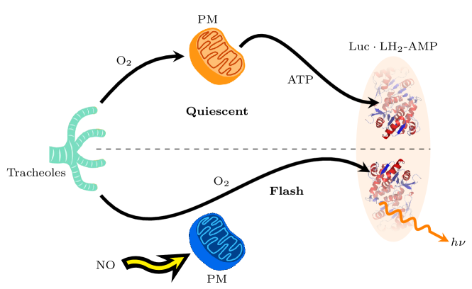
Figure 1: Schematic representation of the NO-controlled lighting mechanism of the firefly inside its lantern.

We now hypothesise that the accumulation of D-Luciferin adenylate $(\ce{Luc.LH}_{2}\textrm{-}\ce{AMP})$, inside the peroxisomes triggers a neurological response which causes activation of NOS. As oxygen is being continuously supplied by the insect through the tracheoles, the trigger must be the critical amount of D-Luciferin adenylate that a firefly makes available for combination with oxygen. This is equivalent to an instability controlled by a trigger parameter, which in this case is the critical D-Luciferin adenylate concentration $x_{c}$ and the trigger can be designed, in its simplest form, as $(x/x_{c}-1)$. It is also experimentally known that if the amount of oxygen that can be pumped to produce oxyluciferin, which produces the flash, is increased, the intensity of the flash grows firefly-oxygen-effect . It can also be understood from the fact that if the oxygen supply to a firefly is cut, the intensity of flash gradually decreases. Therefore, the intensity, which should be proportional to the oxygen concentration, in this case can be thought to be the amplitude of instability and a dynamical relation can be written as,

$$\frac{dy}{dt}=\gamma\left(\frac{x}{x_{c}}-1\right)y,$$ (7)

where $\gamma$ is the growth rate of the equivalent linear instability. We also add a term to take care of some amount of diffusion of oxygen to the peroxisomes assuming that some amount of D-Luciferin adenylate always combines with the available oxygen to produce oxyluciferin. With this, Eq.(7) can be written as

$$\frac{dy}{dt}=\gamma\left(\frac{x}{x_{c}}-1\right)y+\alpha x,$$ (8)

where $\alpha$ is a positive constant. In the above model, the constants $k_{1,2}$ and $\gamma$ are positive constants.

A feedback mechanism and delay

The minimal dynamical model presented by Eqs.(6,8) represents the basic lighting mechanism of a firefly flash, considering one lighting cycle of a firefly. However, we note that the model lacks a basic feedback mechanism, which must be introduced before we can proceed. Consider the reactions given by the reactions (1-3). We see that after de-excitation, oxyluciferin must be converted back to luciferin and then to D-Luciferin adenylate or else oxyluciferin will be continued to be accumulated, which surely does not happen. The details of this conversion process, however is not very well known luciferin-conversion . Also note the reversible nature of the first reaction and both these observations point to the fact that the source term i.e. the first term on the right of Eq.(6) must be a function of $x$, $A\equiv A(x)$, so that the full dynamical equations governing one lighting cycle of a firefly can be written as,

$$\frac{dx}{dt} = k_{1}A(x)-k_{2}xy,$$ (9)

$$\frac{dy}{dt} = \gamma\left(\frac{x}{x_{c}}-1\right)y+\alpha x,$$ (10)

where $A(x)$ is an yet unspecified function of $x$, which can very well be a nonlinear function. We can now understand how this model gives rise to oscillations. Assuming that initially $dx/dt>0$ and $x>x_{c}$, which causes $dy/dt>0$ and $y$ increases. This will eventually make $dx/dt<0$, provided the rate of increase of $k_{1}A(x)$ is less than that of $k_{2}xy$. The variable $y$ continues to increase till $x=x_{c}$, which triggers the emission by making $dy/dt<0$ which causes $y$ to decrease, making $dx/dt>0$ again and the cycle repeats. This model contains all the essential ingredients for an emission cycle except that we still have to come up with a functional form of $A(x)$.

It is well known that time delay is mostly prevalent in biological systems simply because of the reason that biological systems are not connected through mechanisms which can instantly transfer stimuli (or signals) biological-delay1 ; biological-delay2 . We have chosen to introduce time delay in the variable $x$ as

$$\frac{dx}{dt}=k_{1}A(x,x_{\tau_{1}})-k_{2}x_{\tau_{2}}y,$$ (11)

where $x_{\tau_{1,2}}$ are the delayed values of $x\equiv x(t)$ at $t=\tau_{1,2}$, $x_{\tau_{1,2}}\equiv x(t-\tau_{1,2})$. We note that there might be several other places including the neurological response system of the firefly where a time delay might occur, the details are however beyond the scope of this work. The recycling of luciferin after de-excitation of oxyluciferin through the term $A(x)$ suggests that there can be a possible delay in that feedback mechanism, which explains the introduction of delay in $A(x)$. The introduction of the second delay term can be explained through delay in combination of D-Luciferin adenylate with oxygen. For an oscillation cycle to occur, we see that the first term in Eq.(9) must have a stronger dependence on $x$ than the second term if it has to take over the second term to make $dx/dt$ positive so long as the variable $y$ does not increase much. This indicates that $A(x)$ should obey a power law in its simplest form.

Bifurcations and limit cycle — no delay

In this section, we do not consider the time delay and look forward to construct a limit cycle oscillation for our model. Mathematically, a stable limit cycle is an isolated closed orbit of a nonlinear system in the 2-D phase space, which attracts the nearby trajectories strogatz-book . Physically, the existence of a stable limit cycle points to a robust underlying fundamental mechanism, which gives rise to the periodic oscillation.

To normalize Eqs.(9,10), we note that the dimensions of the rate constants $k_{1,2}$, $[k_{1}]=T^{-1}$, which shows that $[A(x)]=[x]$ and $[y]=1$. Besides, the dimension of the growth rate of the trigger mechanism $[\gamma]\equiv[\alpha x]=T^{-1}$. These provide us with the following natural scaling,

$$t \to tk_{1}, x \to xx_{c}, A(x)\to x_{c}A(x),$$

$$\rho =\frac{\gamma}{k_{1}}, \eta =\frac{\alpha x_{c}}{k_{1}}, \beta=\frac{k_{2}}{k_{1}},$$

where we have introduced the dimensionless variables $\rho,\eta,$ and $\beta$, which represent the growth rate of the trigger instability, amount of spontaneous emission, and ratio of the two competing reaction rates. We note that the dimension of $A(x)$ does not prevent it from being a nonlinear function of $x$. With these scaling and variables, we can now write the dynamical model as,

$$\frac{dx}{dt} = A(x)-\beta xy,$$ (12)

$$\frac{dy}{dt} = \rho\left(x-1\right)y+\eta x,$$ (13)

with the constraints $\beta,\rho,\eta>0$.

Linear response

Here, we carry out a linear analysis of the system given by Eqs.(12,13). In order to carry out the analysis, without loss of any generality, we assume a simple power law function for $A(x)=x^{n}$ as described in the before, where $n$ is a positive integer. As mentioned earlier, for an oscillation cycle to occur, the first term on the right hand side of Eq.(12) must have a stronger dependence on $x$ than the second term, we set $n=2$ throughout our analysis. The equations have now two sets of equilibrium points $(x^{\star},y^{\star})$ for Eqs.(12,13),

$$(x^{\star},y^{\star}) = (0,0),$$ (14)

$$= \left(1-\frac{\zeta}{\rho},\frac{1}{\beta}-\frac{\eta}{\rho}\right),$$ (15)

where $\zeta=\beta\eta$. As both $x^{\star},y^{\star}>0$, the only equilibrium point of interest is the second one. Linearsing Eqs.(12,13) around the second equilibrium point, the Jacobian can be obtained as strogatz-book ,

$$J=\left(\begin{array}[]{cc}1-{\displaystyle\frac{\zeta}{\rho}}&-\beta\left(1-{\displaystyle\frac{\zeta}{\rho}}\right)\\ {\displaystyle\frac{\rho}{\beta}}&-\zeta\end{array}\right),$$ (16)

from which we find the trace $(\tau)$ and determinant $(\Delta)$ of the Jacobian as,

$$\tau = 1-\zeta\left(1+\frac{1}{\rho}\right),$$ (17)

$$\Delta = \frac{1}{\rho}(\zeta-\rho)^{2},$$ (18)

from which we can immediately see that $\Delta>0$ always and positivity of $\tau$ depends on the condition,

$$\eta<\eta_{{\rm cr}}=\frac{\rho}{\beta(1+\rho)},$$ (19)

with the limiting value $\eta_{{\rm lim}}\to 1/\beta$ as $\rho\to\infty$. Equivalently, the above condition can also be expressed in terms of a critical $\rho$ value,

$$\rho>\rho_{{\rm cr}}=\frac{\zeta}{1-\zeta},\quad\zeta=\beta\eta<1.$$ (20)

This points to the fact that we have a Hopf bifurcation occurring at $\eta=\eta_{{\rm cr}}$. We have shown the phase portrait of the system in Fig.2. The domain where a Hopf bifurcation is allowed is shown in the first panel of Fig.3. Note that for $n=1$, $\tau=-\zeta\rho/(\zeta+\rho)$, which is always $<0$, so a Hopf bifurcation can never exist and the possibility of a limit cycle can be safely ruled out.

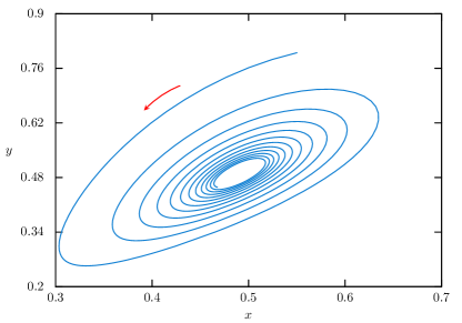
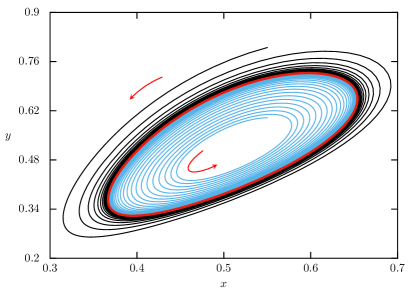
Figure 2: Phase portrait of the system for $\rho=\beta=1$. The left panel shows the behaviour, which is an inward spiral (a sink) above the Hopf bifurcation point, $\eta=0.51$, which is $>\eta_{{\rm cr}}$. The right panel shows the phase portrait after Hopf bifurcation occurs at $\eta_{{\rm cr}}$, for $\eta=0.49$. The thick red colour line shows the resultant limit cycle.

From the inspection of the phase portrait, we conclude that a supercritical Hopf bifurcation occurs at $\eta=\eta_{{\rm cr}}$, following which a limit cycle appears (see the next section). The eigenvalues of the Jacobian are given by $\lambda=\gamma\pm i\omega$, with

$$\gamma = \frac{1}{2\rho}[\rho-\zeta(1+\rho)],$$ (21)

$$\omega = \frac{1}{2\rho}\left[\rho^{2}(1-4\rho)-2\zeta\rho(1-3\rho)+\zeta^{2}(1-\rho)^{2}\right]^{1/2},$$ (22)

so that the time period $T$ of the limit cycle in the vicinity of $\eta\simeq\eta_{{\rm cr}}$ is given by,

$$T=\frac{2\pi}{\omega}+{\cal O}(\eta-\eta_{{\rm cr}}).$$ (23)

For the parameter $\beta=\rho=1,\eta=0.49$, the period of the limit cycle is found to be $\simeq 13$, which is very close to the predicted value $T=12.33$ calculated from Eq.(23).

Invariant region

Assuming $A(x)=x^{2}$, we now construct a positive invariant region around the equilibrium point of the system represented by Eqs.(12,13). Consider the figure shown in the second panel of Fig.3. The system has three null-clines, two of which are shown in the figure.

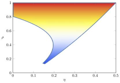
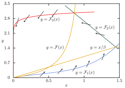
Figure 3: Allowed domain for Hopf bifurcation in the $(\rho,\eta)$ plane. The parameters are same as in Fig.2. A positive invariant region for Eqs.(12,13) around its equilibrium point.

$$x = 0,$$ (24)

$$y = x/\beta,$$ (25)

$$y = \frac{\eta x}{\rho(1-x)}={\cal F}(x).$$ (26)

and

$$\frac{dy}{dx}=\frac{\rho(x-1)y+\eta x}{x^{2}-\beta xy}.$$ (27)

Consider now a family of curves $y={\cal F}_{i}(x)$, given by

$${\cal F}_{1} = \frac{ax}{1+x}+bx^{4},$$ (28)

$${\cal F}_{2} = -mx+c,$$ (29)

$${\cal F}_{3} = \frac{dx^{p}}{1+x^{p}},$$ (30)

with certain chosen parameters $a,b,m,c,d,p>0$, such that

$$a,b < {\cal M},$$ (31)

$$m,d > {\cal N},$$ (32)

$$p < 1,$$ (33)

where ${\cal M}$ and ${\cal N}$ are two arbitrary large positive numbers. It can now be shown that in all the regions around the equilibrium point, the flow is always anti-clockwise into the region, spanned by these three curves, so that a positively invariant region can be constructed around the equilibrium point. The region is schematically shown in Fig.3. The Poincaré-Bendixson theorem strogatz-book ; Holmes-book now tells us that the invariant region contains a unique limit cycle.

Parameterisation and comparison — no delay

In this section, we parameterise our model for $n=2$ without any time delay and compare the numerical results with available data. For comparison, we take the data from the work of Sharma et al. firfely-male , where they report about the temperature dependence on the flash duration of male fireflies Luciola praeusta, found in the northeastern Indian state of Assam. In this work, the authors study the change in the amplitude and duration on ambient temperature for a live firefly. The actual experimental data for three ambient temperatures of $20\,{\rm{}^{\circ}C}$, $30\,{\rm{}^{\circ}C}$, and $40\,{\rm{}^{\circ}C}$ are shown in Fig.5. Overall, a few changes are observed — as the ambient temperature increases, the sharpness of the flashes are found to increase (or a decreasing flash width), while the average amplitude of a pulse and the duration of a lighting cycle are found to decrease. In what follows, we try to estimate the numerical parameters on the basis of the experimental data presented in Fig.5. There is also a companion work by the same authors on the females of the same species firfefly-female . We however could not find any consistent behaviour of the flash patterns for female fireflies with respect to their pulse width, amplitude, and period as temperature changes in the lighting pattern of the females.

Before we proceed, it is worth looking at the behaviour of the flash. As can be seen from the experimental data, a lighting cycle contains a fast and a slow manifold. Most of the time the cycle spends its time on the slow manifold. A flash occurs on the fast manifold. In the first panel of Fig.4, the numerical solution of the variable $x(t)$ and $y(t)$ are shown (blue and red thick curves) for one flash. Note that $y(t)$ represents the intensity of the flash, which can be approximated with an exponential function

$$y(t)\sim\varepsilon e^{-\mu(t-t_{0})^{2}}+\delta,$$ (34)

centered around $t=t_{0}$, with the constants $\varepsilon,\mu,\delta>0$, which is shown as the thin green curve with the best fitted parameters. We note that the width or sharpness of the pulse is directly proportional to $\mu$. The corresponding solution for $x(t)$ can be found in terms of error function as,

$$x(t)\sim\frac{{\cal P}(t)}{{\cal C}-\int_{1}^{t}{\cal P}(\tau)\,d\tau},\quad{\cal P}(t)=\exp\left[-\delta\beta t-\frac{1}{2}\varepsilon\beta\sqrt{\frac{\pi}{\mu}}{\rm erf}\left\{\sqrt{\mu}(t-t_{0})\right\}\right],$$ (35)

where ${\cal C}$ is an integration constant. For the fitted parameters, this approximation is plotted in the panel as the black thin curve and from the figure, we see that these analytical approximations for both $(x,y)$ work quite well during a flash. Putting back the analytical approximation for $y(t)$ as given by Eq.(34) in our dynamical model, we see that $\rho\sim 2\mu$ is the parameter which controls the sharpness of the flash or the width of the pulse — the larger is the value of $\rho$, the sharper is the flash or the narrower is the width of the flash.

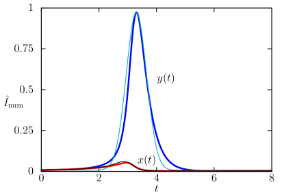
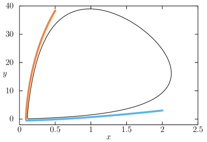
Figure 4: The first panel shows the analytical approximations to the numerical reproduction of the flash with the numerical intensity normalised to unity. The slow manifold of the lighting cycle in the $(x,y)$ phase space is shown in the second panel.

Based on the above analysis, we assume that the firefly flash is a result of a linear instability of growth rate $\gamma$, which can be estimated from the experimental data by calculating how quickly the the flash peaks up. If $I_{{\rm peak}}$ is the peak intensity of a flash with a rise time (from zero) of $\Delta t_{{\rm rise}}$, then

$$\frac{\Delta I}{\Delta t_{{\rm rise}}}\sim\gamma e^{\gamma t},\quad\Delta I\equiv I_{{\rm peak}},$$ (36)

where $I\sim e^{\gamma t}$, from which $\gamma$ can be estimated as

$$\gamma\sim\frac{1}{\Delta t_{{\rm rise}}}\frac{I_{{\rm peak}}}{I_{{\rm av}}}\sim\frac{2}{\Delta t_{{\rm rise}}},$$ (37)

where $I_{{\rm av}}\equiv I_{{\rm peak}}/2$ is the average intensity of the flash.

In order to have an idea about period of the lighting cycle, we observe that the duration of a lighting cycle is determined by the slow manifold of the cycle. In the second panel of Fig.4, the phase portrait of a complete lighting cycle is shown. We note that the amplitude of the variable $x(t)$ remains quite low compared to that of $y(t)$. It can be numerically ascertained that the slow manifold consists of a long vertical drop of the variable $y(t)$ and a near horizontal stretch of $x(t)$, which are shown in second panel of Fig.4 as orange and blue coloured thick lines. On the vertical manifold, we can approximate the time as

$$\tau_{{\rm vert}}\approx\int_{y_{i}}^{y_{f}}\left.\frac{dt}{x^{2}-\beta xy}\right|_{x\to\beta y}\sim\frac{1}{p}\left[\ln\left(\frac{y_{i}}{y_{f}}\right)+\ln\left(\frac{p-y_{f}\beta\rho}{p-y_{i}\beta\rho}\right)\right],$$ (38)

where $y_{i,f}$ is the initial and final values of $y(t)$ on the vertical drop and the parameter $p=\rho-\beta\eta$. On the horizontal manifold, the time spent in the phase space can be approximated as

$$\tau_{{\rm hor}} \approx \int_{x_{i}}^{x_{f}}\left.\frac{dt}{\rho(x-1)+\eta x}\right|_{y\to\eta x\rho^{-1}/(x-1)},$$ (39)

$$\sim \frac{\rho}{x_{i}x_{f}p^{2}}\left[p(x_{f}-x_{i})+x_{i}x_{f}\beta\eta\left\{\ln\left(\frac{x_{f}}{x_{i}}\right)+\ln\left(\frac{p-x_{i}\rho}{p-x_{f}\rho}\right)\right\}\right],$$

where $x_{i,f}$ is the initial and final values of $x(t)$ on the horizontal stretch. So, the approximate time spent on the slow manifold is

$$\tau_{{\rm slow}}\sim\tau_{{\rm vert}}+\tau_{{\rm hor}}\propto(\rho-\beta\eta)^{-1}.$$ (40)

Or, in other words, the period of a lighting cycle should be inversely proportional to the quantity $(\rho-\beta\eta$).

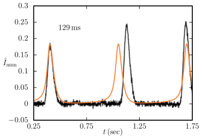
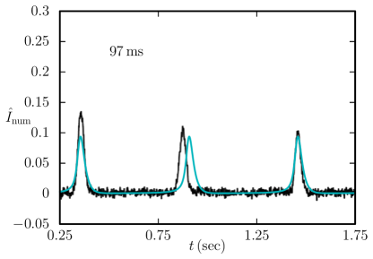
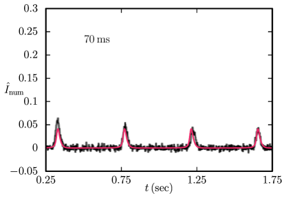
Figure 5: Comparison of numerical results with experimental data. The solid coloured lines are the results of the numerical model, superimposed with the corresponding experimental images firfely-male . The values (inset) indicate the width of the flash.

With the value of $\gamma=\gamma_{{\rm expt}}$ estimated from the experimental data as described above and with Eq.(40), we parameterise the model given by Eqs.(12,13) for the free parameters $k_{1,2},\eta$, for an optimum fit, subject to the constraints $\eta<\eta_{{\rm lim}},\gamma=\gamma_{{\rm expt}}$, where we minimise the quantity

$$\epsilon=\frac{1}{2}\left(\left|\hat{I}_{{\rm num}}-\bar{I}_{{\rm peak}}\right|+\left|t_{{\rm num}}-t_{{\rm period}}\right|\right),$$ (41)

which is the combined, average absolute fitting error with respect to the amplitude and period of the pulse, where $t_{{\rm num}}$ is the numerical period, $t_{{\rm period}}$ is the period found from the experimental data, $\hat{I}_{{\rm num}}$ is the numerical amplitude of the flash, and $\bar{I}{}_{{\rm peak}}$ experimental peak intensity. The numerical fits to the available experimental data are shown in Fig.5., as solid colour lines. The fitted parameters are listed in Table.1.

Table 1: Parameterisation of numerical model.

Temp.	$t_{{\rm period}}$	$t_{{\rm flash}}$	$\gamma$	$k_{1}$	$k_{2}$	$\eta_{{\rm lim}}$	$\eta$	$\bar{I}{}_{{\rm peak}}$	$\hat{I}_{{\rm num}}$		$\rho$	$\beta$	$t_{{\rm num}}$
$20\,{\rm{}^{\circ}C}$	$0.646$	$0.129$	$39.63$	$22$	$1.15$	$12.30$	$8.20$	$0.183$	$0.183$		$1.80$	$0.052$	$14.21$
$30\,{\rm{}^{\circ}C}$	$0.548$	$0.097$	$58.41$	$24$	$3.42$	$5.03$	$2.06$	$0.116$	$0.094$		$2.43$	$0.143$	$13.15$
$40\,{\rm{}^{\circ}C}$	$0.442$	$0.070$	$91.24$	$27$	$12.0$	$1.74$	$0.67$	$0.051$	$0.041$		$3.38$	$0.444$	$11.93$

In the table, the $\hat{I}_{{\rm num}}$ is the numerical amplitude of the flash, normalised by the average experimental peak intensity $\bar{I}{}_{{\rm peak}}$ for $20\,{\rm{}^{\circ}C}$ with $\epsilon_{{\rm max}}=0.5$.

The best fit parameters indicate that the reaction rates $k_{1,2}$ increase with temperature, which for any reactions involving enzymes, is expected to be true pyrosequencing . It is also interesting to note that the experimentally reported values for the reaction rates $k_{1,2}$ for firefly luciferase are $19.2\,{\rm s}^{-1}$ and $0.96\,{\rm s}^{-1}$ respectively pyrosequencing , which are of the same order as our numerically fitted values (see Table.1) for $20\,{\rm{}^{\circ}C}$. In the same report, it is also reported that the Pyrosequencing experimental data predicts $k_{1}=30\pm 10\,{\rm s}^{-1}$ and $k_{2}=10\pm 3\,{\rm s}^{-1}$, with a significant change in the value of $k_{2}$ pyrosequencing . Interestingly, the Pyrosequencing data are of the same order for our numerically fitted values at higher temperature. As can be seen from Fig.5, our fitted results most agree with the experimental data at higher temperatures, namely at $40\,{\rm{}^{\circ}C}$ and as reported in the paper by Sharma et al. firfely-male , the natural flashing temperature of these fireflies lies within $27-32\,{\rm{}^{\circ}C}$, which is the ambient temperature of the habitats where these fireflies are found.

Effect of delay

In this section, we examine what happens to the lighting cycle, when the combination of oxygen with D-Luciferin adenylate as well as the conversion of oxyluciferin to luciferin through the feedback cycle are delayed

$$\frac{dx}{dt} = xx_{\tau_{1}}-\beta x_{\tau_{2}}y=f(x,x_{\tau_{1}},x_{\tau_{2}},y),$$ (42)

$$\frac{dy}{dt} = \rho\left(x-1\right)y+\eta x=g(x,y),$$ (43)

where $x_{\tau_{1,2}}\equiv x(t-\tau_{1,2})$ represent the value of the variable $x$ at an earlier times $t-\tau_{1,2}$, with $\tau_{1,2}$ being the delays. The equilibrium point of interest is given by

$$(x^{\star},y^{\star})=\left(1-\frac{\zeta}{\rho},\frac{1}{\beta}-\frac{\eta}{\rho}\right).$$ (44)

Following standard procedure Rand ; Roussel , we now expand the variables about the equilibrium point,

$$\bm{x} = \bm{x}^{\star}+\delta\bm{x}$$ (45)

$$\dot{\bm{x}} = \delta\dot{\bm{x}}=\bm{f}\left(\bm{x}^{\star}+\delta\bm{x},\bm{x}^{\star}+\delta\bm{x}_{1},\bm{x}^{\star}+\delta\bm{x}_{2}\right),$$ (46)

where $\delta x$ and $\delta y$ are the respective small deviations of the variables at time $t$, with

$$\bm{x} = (x,y)^{\prime},$$ (47)

$$\delta\bm{x} = (\delta x,\delta y)^{\prime},$$ (48)

$$\bm{f} = (f,g)^{\prime},$$ (49)

where $()^{\prime}$ denotes the transpose of a row vector. The deviations $\delta\bm{x}_{1,2}$ represent the deviations at the delayed time $t-\tau_{1,2}$. Expanding and linearising Eqs.(42,43) about the equilibrium point, we have

$$\delta\dot{\bm{x}}\simeq\bm{J}_{0}\,\delta\bm{x}+\bm{J}_{1}\,\delta\bm{x}_{1}+\bm{J}_{2}\,\delta\bm{x}_{2},$$ (50)

where $\bm{J}_{0,1,2}$ are the linearised Jacobians with respect to time $t$ (no delay) and delayed time $t-\tau_{1,2}$,

$$\bm{J}_{0} = \left(\begin{array}[]{cc}1-{\displaystyle\zeta/\rho}&-\beta+{\displaystyle\beta\zeta/\rho}\\ {\displaystyle\rho/\beta}&-\zeta\end{array}\right),$$ (53)

$$\bm{J}_{1} = \left(\begin{array}[]{cc}1-\zeta/\rho&0\\ {\displaystyle 0}&0\end{array}\right),$$ (56)

$$\bm{J}_{2} = \left(\begin{array}[]{cc}-1+\zeta/\rho&0\\ {\displaystyle 0}&0\end{array}\right),$$ (59)

Eq.(50) represents the linear delay differential equation (DDE) corresponding to the DDE Eqs.(42,43). Assume now that the deviations $\delta\bm{x}(t)$ has an exponential solution of the form

$$\delta\bm{x}(t)\sim\bm{A}e^{\lambda t}.$$ (60)

Substituting the above trial solution to the linear DDE, we arrive at the characteristic equation

$$\left|\bm{J}_{0}+e^{-\lambda\tau_{1}}\bm{J}_{1}+e^{-\lambda\tau_{2}}\bm{J}_{2}-\lambda\bm{I}\right|=0,$$ (61)

which should possess complex solutions of the type $\lambda=\gamma\pm i\omega$. We now look for the possibility of having a pair of pure imaginary eigenvalues $\lambda=\pm i\omega$, giving rise to a Hopf bifurcation Rand ; Roussel . At the Hopf point, separating the real and imaginary parts of the the characteristic equation, we have,

$$(\zeta-\rho)[\zeta c_{1}+\omega s_{1}]+(\zeta-\rho)^{2}-\rho\omega^{2} = 0,$$ (62)

$$\omega[(\zeta-1)\rho+\zeta]-(\zeta-\rho)[\zeta s_{1}-\omega c_{1}] = 0,$$ (63)

where

$$\cos(\omega\tau_{1})-\cos(\omega\tau_{2}) = c_{1},$$ (64)

$$\sin(\omega\tau_{1})-\sin(\omega\tau_{2}) = s_{1}.$$ (65)

Double peak pulse

We would now like to note the occurrence of pulse with multiple peaks, especially the occurrence of double peak pulse at low temperature firfely-double-peak . Following the trends of dependence of various parameters on temperature (see Table.1) we look for a regime with temperature lower than $20^{\circ}\,{\rm C}$, where multiple peak pulse may occur with the constraints $\rho<1.80,\beta<0.052,\eta>8.20,$ and $t_{{\rm num}}>14.21$.

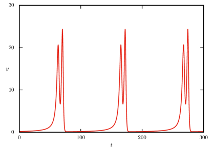
Figure 6: The phase portrait of a double-peak pulse is shown in the first panel and the corresponding pulse for the parameters $\rho=1.53,\beta=0.045,\eta=9.9,\tau_{1}=3.4,\tau_{2}=2.805$ is shown in the second panel.

As an example, we find that the parameter regime $\rho=1.53,\beta=0.045,\eta=9.9$ with $\tau_{1}=3.4$ and $\tau_{2}=2.805$ results a double peak pulse as shown in the Fig.6. Interestingly this double-peak pulse is surrounded by chaotic oscillations on both sides. To explore the bifurcation of Eqs.(42,43) with these parameters, taking $\rho$ as the free parameter, we plot the orbit diagram (a plot of maxima of $y$, $y_{{\rm max}}$ versus $\rho$), starting from the Hopf point, along with the corresponding maximal Lyapunov exponent $\sigma_{M}$ delay-technique (first panel of Fig.7). The Hopf point can be found by solving Eqs.(62,63) for the given parameters for the variables $(\rho,\omega)$, which yields the solutions $\rho\simeq 1.00251,\omega\simeq 0.69$. A plot of the real part of the eigenvalue versus $\rho$, showing the Hopf point is also shown in the second panel of Fig. 7. As can be seen from the orbit diagram that the first period doubling bifurcation following the Hopf bifurcation occurs at $1.003$ and the subsequent period doubling bifurcation occurs at $1.159$. After that the system follows the usual route to chaos through a series of period doubling bifurcations strogatz-book , also characterised by the maximal Lyapunov exponent. This chaotic regime continues till $\rho\simeq 1.4$ after which a stable two-period pulse appears, which is our characteristic pulse regime at low temperature. Beyond $\rho=1.55,$ the system exhibits bouts of chaotic regimes and stable periodic oscillations akin to logistic maps.

Summary

To summarise, we have constructed a low dimensional model for the emission of firefly flash. We have compared our numerical findings with the existing experimental results firfely-male . Though our model has certain limitations, it successfully explains the experimental results describing the effect of temperature on amplitude and period of the firefly flash. Our model is able to predict the rate constants $k_{1}$ and $k_{2}$, which nearly agrees with the existing experimental pyrosequencing data pyrosequencing . Comparing our numerical results with the experimental data firfely-male , we conclude that $k_{1}$ and $k_{2}$ both tend to increase with temperature due to the rapidity of the production of the $\ce{Luc.LH}_{2}\textrm{-}\ce{AMP}$ inside the peroxisomes in quiescent phase of the lighting cycle and in the flash phase inside the light emitting organ, $k_{2}$ is found to be increases more rapidly compared to $k_{1}$, as it is the rate constant for the production of light and as the production of $\ce{Luc.LH}_{2}\textrm{-}\ce{AMP}$ is larger in high temperature and oxygen is being continuously supplied by the tracheoles, it obviously produces more light causing increase in $k_{2}$, i.e. $\beta$ increases abruptly with temperature resulting increase in the sharpness of the peak and decrease in the amplitude of a pulse and the duration of a lighting cycle.

Addition of time delay in our model explains low temperature behavior of the firefly flash pattern. At low temperature firfefly-female ; firfely-double-peak , the firefly enzymatic catalytic reaction becomes slower and slower with decreasing temperature resulting broadening of the peaks (distorted into two or more than two peaks) and increase in the duration of the lighting cycle. At lower temperature, $k_{1}$ for the production of $\ce{Luc.LH}_{2}\textrm{-}\ce{AMP}$ at some earlier time is found to be smaller compared to other non delayed case which obeying the slowness of the reaction. Here, oxygen supplied in present time is large enough compared to the past time that it combines with the delayed $\ce{Luc.LH}_{2}\textrm{-}\ce{AMP}$ resulting increase in $k_{2}$ with a larger duration of flash with distorted peaks. Numerically, formation of double peak at low temperature can be explained by the period doubling bifurcation followed by a Hopf bifurcation. For the delayed model, we produce a double peak following the trends of approximate parameter values taken at non-delayed case. Maximal Lyapunov exponent is further calculated for the delayed firefly model and positive Lyapunov exponents implies the existence of chaotic regime. We have found lots of local regime where multiple orbits are found and it is believed to be controlled by firefly itself through the neurological responses.

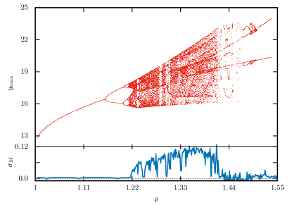
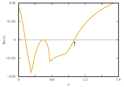
Figure 7: 1st panel : The orbit diagram ($y_{{\rm max}}$ versus $\rho$) for the parameters $\beta=0.045,\eta=9.9,\tau_{1}=3.4,\tau_{2}=2.805$. The corresponding maximal Lyapunov exponent $(\sigma_{M})$ is plotted in the lower panel of the plot. 2nd panel : Plot of the real part of the eigenvalue ${\rm Re(\lambda)}$ is shown against the free parameter $\rho$. The arrow mark shows the position of the Hopf point.

Appendix

Approximation of a DDE system

As we know that a dynamical system with time delay is basically an infinite dimensional system, the delay system can be reduced to a set of $N$ ordinary differential equations, where $N$ is a large positive integer delay-technique .

Consider our DDE with two delays $\tau_{1,2}$,

$$\frac{dx}{dt} = f[x(t),x(t-\tau_{1}),x(t-\tau_{2}),y(t)],$$ (66)

$$\frac{dy}{dt} = g[x(t),y(t)],$$ (67)

assuming $\tau_{1}>\tau_{2}$ numerically. We now divide the larger of the delay into $N$ different discrete divisions, each of size $\Delta t$ such that $\Delta t=\tau_{1}/N$ or equivalently $N=\tau_{1}/\Delta t$. As $N\gg 1$, $\Delta t$ is very small so that we have,

$$x(t+\Delta t)\simeq x(t)+\Delta t\,f[x(t),x(t-N\Delta t),x(t-M\Delta t),y(t)],$$ (68)

where $M\,(<N)$ is an integer such that $M=\tau_{2}/\Delta t$ (please see explanation about $M$ at the end of this section). Denoting now the values of $x(t)$ at a discrete time $t_{j}$ as $x_{j}(t)$, we have,

$$x_{j+1}(t)=x_{j}(t-\Delta t),$$ (69)

which can be written as

$$x_{j+N}(t) = x_{j}(t-N\Delta t),$$

$$\Rightarrow x_{N}(t) = x_{0}(t-N\Delta t),$$ (70)

so that we can have now

$$\frac{d}{dt}x_{0}(t)=f[x_{0}(t),x_{N}(t),x_{M}(t),y(t)].$$ (71)

Following this prescription, we can now write the original DDE system as,

$$\frac{dx_{0}}{dt} = f(x_{0},x_{N},x_{M},y),$$ (72)

$$\frac{dx_{j}}{dt} = \frac{N}{2\tau_{1}}(x_{j-1}-x_{j+1}),\quad 1\leq j\leq N-1,$$ (73)

$$\frac{dx_{N}}{dt} = \frac{N}{\tau_{1}}(x_{N-1}-x_{N}),$$ (74)

$$\frac{dy}{dt} = g(x_{0},y),$$ (75)

for $N\gg 1$, which can now be solved with any standard method. For $N\to\infty$, the above system will reduce to the original DDEs.

One important point to be noted here about the value of $N$. While any large positive integer as a value of $N$ will do for a single delay DDE system, for a system with double delays such as in our case, it is important that the difference between the two delays $(\tau_{1}-\tau_{2})$, assuming $\tau_{1}>\tau_{2}$, is exactly divisible by $\Delta t$ for the chosen value of $N$. This is required as we have now divided the entire time interval $[0,\tau_{1}]$ into discrete divisions, the smaller of the delays, which in this case is $\tau_{2}$ falls exactly at one node, otherwise the discrete set of equations will not maintain the analytical difference between the delays for small values of $N$. In our chosen set of values of $\tau_{1}=2.53$ and $\tau_{2}=2.3$, $N$ should be a multiple of $11$. If the difference between the delays is not exactly divisible by $\Delta t$, $N$ should be large enough to make the this difference equivalent to the analytical value, otherwise even a small value of $N$ gives quite good results.

References

- (1) J. L. Capinera, Encyclopedia of Entomology, Springer, 2008.
- (2) Y. Ando et al., Nature Photonics 2, 44 (2008).
- (3) D. W. Ow et al., Science 234, 856 (1986).
- (4) S. J. Gould and S. Subramani, Anal. Biochem. 175, 5 (1988).
- (5) L. J. Kricka, Clin. Chem. 37, 1472 (1991).
- (6) J. Buck and E. Buck, Sci. Am. 234, 74 (1976).
- (7) R. L. Airth and G. E. Foerster, Archives Biochem. Biophys. 97, 567 (1962).
- (8) A. G. Oliveira and C. V. Stevani, Photochem. Photobio. Sci. 8, 1416 (2009).
- (9) K. V. Wood, Photochem. Photobiol. 62, 662 (1995).
- (10) J. C. Day, L. C. Tisi, and M. J. Bailey, Luminescence 19, 8 (2004).
- (11) O. Shimomura, F. H. Johnson, and Y. Kohama, Proc. Nat.Acad. Sci. USA 69, 2086 (1972).
- (12) H. M. Smith, Science 82, 151 (1935).
- (13) R. E. Mirollo and S. H. Strogatz, SIAM J. Appl. Math. 50, 1645 (1990).
- (14) W. D. McElroy, H. H. Seliger, and E. H. White, Photochem. Photobiol. 10, 153 (1969).
- (15) F. McCapra, Acc. Chem. Res. 9, 201 (1976).
- (16) B. A. Trimmer et al., Science 292, 2486 (2001).
- (17) J. R. Aprille et al., Integr. Comp. Biol. 44, 213 (2004).
- (18) Y.-L. Tsai et al., Phys. Rev. Lett. 113, 258103 (2014).
- (19) H. Fraga, Photochem. Photobio. Sci. 7, 146 (2008).
- (20) M. M. Rabha et al., J. Photochem. Photobiol. B 170, 134 (2017).
- (21) A. Goswami, P. Phukan, and A. G. Barua, J. Fluroscence 29, 505 (2019).
- (22) U. Sharma et al., Photochem. Photobiol. Sci. 13, 1788 (2014).
- (23) A. Agah et al., Nucleic Acids Res. 32, e166 (2004).
- (24) H. H. Seliger and W. D. McElroy, Proc. Nat. Acad. Sci. 52, 75 (1964).
- (25) J. W. Hastings, Cell Physiology Source Book, chapter Bioluminescence, pages 665–681, Academic Press, New York, 1995.
- (26) T. Hirano et al., J. Am. Chem. Soc. 131, 2385 (2009).
- (27) J. W. Hastings, W. D. McElroy, and J. Coulombre, J. Cell. Comp. Physio. 42, 137 (1953).
- (28) K. Okada et al., Tetrahad. Lett. 15, 2771 (1974).
- (29) G. Orosz, J. Moehlis, and R. M. Murray, Phil. Trans. Royal Soc. A 368, 439 (2010).
- (30) U. an der Heiden, J. Math. Biol. 8, 345 (1979).
- (31) S. H. Strogatz, Nonlinear dynamics and chaos: with applications to physics, biology, chemistry, and engineering, CRC Press, 2018.
- (32) J. Guckenheimer and P. J. Holmes, Nonlinear Oscillations, Dynamical Systems, and Bifurcations of Vector Fields, Springer, 1983.
- (33) R. Rand, Complex Systems : Fractionality, Time-delay and Synchronization, chapter 3, pages 83–117, Springer, 2012.
- (34) M. R. Roussel, Nonlinear Dynamics : A hands-on introductory survey, IOP, 2019.
- (35) M. Lakshmanan and D. V. Senthilkumar, Dynamics of nonlinear time-delay systems, Springer, 2011.