Isotropic All-electric Spin analyzer based on a quantum ring with spin-orbit couplings

Abstract

Here we propose an isotropic all electrical spin analyzer in a quantum ring with spin-orbit coupling by analytically and numerically modeling how the charge transmission rates depend on the polarization of the incident spin. The formalism of spin transmission and polarization rates in an arbitrary direction is also developed by analyzing the Aharonov-Bohm and the Aharonov-Casher effects. The topological spin texture induced by the spin-orbit couplings essentially contributes to the dynamic phase and plays an important role in spin transport. The spin transport features derived analytically has been confirmed numerically. This interesting two-dimensional electron system can be designed as a spin filter, spin polarizer and general analyzer by simply tuning the spin-orbit couplings, which paves the way for realizing the tunable and integrable spintronics device.

I Introduction

Manipulation of the spin degrees of freedom and the conduction charges in low-dimensional quantum structures has been attracting considerable interest, due to wide range of potential applications in semiconductor spintronics and quantum computation. How to control, modulate, or detect the spin degree of freedom at the mesoscopic scale is a key step for the application of the spin coherence in electronic devices. The quantum ring chapter ; ring1 is an ideal platform to take into consideration the Aharonov-Bohm (AB) and the Aharonov-Casher (AC) effects to show the nature of the quantum interference in conductance. The transport properties of similar nano-devices have received considerable attention, especially in the spin transport device subject to the Rashba spin-orbit coupling (SOC) datta ; sun ; chi ; chang ; transport ; chuang , but the presence of Dresselhaus SOC or combination of both SOCsmiao ; sil have not been investigated sufficiently as yet.

The interplay of the Rashba SOC and the quantum interference has been widely reported in the literature. No spin is being polarized Nitta ; AC3 ; AC5 in the transmission in the two-lead rings with equal arm length and without a magnetic flux or an impurity. This is because in this case the interference phase of the two different eigentransport channels is entirely due to the AC effect. The signs of phases are opposite but the absolute values are equal resulting in equal transmission rate for opposite spins. To polarize the spin, we need to introduce magnetic fields Gumber ; AC1 ; AC2 ; Lucignano , use unequal length arms Nitta ; Wang ; Tang , doping Bellucci ; Citro ; Kovalev , or contact three or more leads Saeedia ; Zhai .

Quantum interference between the two arms of the ring provides suitable means for controlling the spin in the nano-scale, which has been proven by the Green’s function method Wang ; Sun1 or Griffith’s boundary conditions Griffith ; AC1 ; Bellucci ; Citro ; Tang ; Saeedia ; Zhai . The first order linear approximation with full transparent contacts was also reported Nitta ; AC2 ; Gumber ; Li , albeit without the backscattering effect. The S-matrix method Hatano ; Naeimi presents a rough assessment of the backscattering by fixing the energy-dependent coupling parameter between the leads and ring as constant. We note that previous works on spin transport properties in the quantum ring were not comprehensive. For spin-unpolarized input current these works often only focused on spin polarization in the $z$ direction or the direction of the eigenstates of the ring. The total polarizability, polarization direction, and spin polarization in arbitrary directions were rarely discussed. Work in the case of the arbitrarily spin-polarized incident are difficult to find in the literature.

In this work, we present an analytical model for one-dimensional (1D) rings and numerical studies of realistic two-dimensional (2D) quantum rings in the non-equilibrium Green’s function (NEGF) method chang where both the Rashba and Dresselhaus SOCs are present. We derive the formula for the transmission rates for arbitrary spin polarization and generalize them to the cases of the polarized incident spin. A density matrix describing the spin-polarized (in arbitrary direction) input current is also introduced into the Green’s function equation, which results in the same results obtained by the analytical 1D model. The transmission rate $T$ can be up to unity with the fully polarized output in a proper magnetic field and with a proper Rashba SOC.

When the input current is spin-polarized the transmission rate depends on the direction of the input polarization and the output current is still spin polarized. So the quantum ring is also acting as a spin torque which may be useful in spintronics. This property also guides us finding the way to design an omnidirectional spin analyzer. In contrast, the optical polarization analyzer is simpler since the polarization is perpendicular to the direction of the light. However, the spin polarization can be along an arbitrary direction on the Bloch sphere. The spin analyzer in a particular direction can be achieved in the ferromagnetism systems handbook . The arbitrary spin analyzer needs the light involved huang ; jozwiak , which is difficult to be integrated. Here, we just need to measure the conductances in different strengthes of the SOC to obtain the polarization of the incident spin, which is easier to integrate on the chip. It is interesting that in such a simple system, the spin filter, spin polarizer and spin analyzer can be achieved by just tuning the magnetic field or the Rashba SOC via the gate Rash01 ; Rash03 ; Rash04 ; Rash05 .

II The transport properties in the one-dimensional model

To understand the transport properties in a quantum ring, the one-dimensional (1D) model is usually applied. The ring is contacted with the left and the right leads at $\varphi=\pi$ and $0$, respectively. In this work, we suppose that the electron is injected from the left lead, then it travels through the ring in two different paths, one from $\varphi=\pi$ to $0$ clockwise (the upper arm) and the other from $\varphi=\pi$ to $2\pi$ counterclockwise (the lower arm), as shown in Fig. 1(a).

As discussed in the previous work peng , the 1D model works very well when the radius is not too large. The 1D model here, at least, is a good approximation which results in the correct physical pictures. Another approximation of neglecting the Zeeman effect is also adopted. In the relatively low magnetic field ($B<3$T), the Zeeman coupling is weak and could be neglected. We can also numerically verify that this approximation is appropriate in low magnetic fields.

For simplicity, we first consider only the Rashba SOC being present. If the Zeeman coupling is neglected the energy spectrum of the 1D ring is given by sheng ; AC1 ; AC2 ; AC3 ; AC4 $E_{n}^{\mu}=\tau\left(n_{j}^{\mu}-\frac{\Phi_{AB}}{2\pi}-\frac{\Phi_{AC}^{\mu}}{2\pi}\right)^{2}$ where $n_{j}^{\mu}$ is the orbital quantum number, and the index $\mu=1,2$ represents the spin eigenstates $\left|\uparrow\right\rangle$ and $\left|\downarrow\right\rangle$, and $j=\pm$ represents the clockwise and counterclockwise electron motions, respectively. Also, $\tau=\frac{\hbar^{2}}{2m^{*}r_{0}^{2}}$ is the energy unit, $\Phi_{AB}=2\pi N$ is the AB phase with the relative magnetic flux $N=\frac{eBr_{0}^{2}}{2\hbar}$, and $\Phi_{AC}^{\mu}=(-1)^{\mu}\left(\sqrt{1+4\beta_{1}^{2}}-1\right)\pi$ is the AC phase with $\beta_{1}=g_{1}m^{*}r_{0}/\hbar$.

The corresponding eigenstates are given by $\Psi_{j}^{\mu}\left(\varphi\right)=\frac{1}{\sqrt{2\pi}}e^{-in_{j}^{\mu}\varphi}\chi^{\mu}\left(\varphi\right)$, where $\chi^{1}(\varphi)=\left(\cos\frac{\theta_{1}}{2},-e^{i\varphi}\sin\frac{\theta_{1}}{2}\right)^{T}$ and $\chi^{2}(\varphi)=\left(\sin\frac{\theta_{1}}{2},e^{i\varphi}\cos\frac{\theta_{1}}{2}\right)^{T}$, with $\tan\theta_{1}=2\beta_{1}$ AC4 . It is clear that the directions of the spin polarization are along $(\theta_{1},\varphi)$ and $(\pi-\theta_{1},\pi+\varphi)$ for the two eigenstates respectively.

The schematic diagram of the total transport is explicitly drawn in Fig. 1(a). The incident current can be decomposed into the two eigenstates $\chi^{1,2}$, and the electron is transported by these two channels. The transmission rate is given by (see the Method),

$$T_{\mu}=\frac{K\Phi^{\mu}}{KK^{\prime}+\left[4k_{0}^{2}\left(\Phi^{\mu}-K^{\prime}\right)+k^{2}\sin^{2}(\pi k_{0}r_{0})\right]^{2}},$$ (1)

where $K=16k^{2}k_{0}^{2}\sin^{2}(\pi k_{0}r_{0})$, $\Phi^{\mu}=\cos^{2}\frac{\Phi_{AB}+\Phi_{AC}^{\mu}}{2}$ and $K^{\prime}=\cos^{2}(\pi k_{0}r_{0})$. For vanishing magnetic field the AB phase vanishes and the SOC induced energy shift $U_{0}$ is neglected, then Eq. (1) agrees with the results obtained in Ref. AC1 ; AC3 . If there is a constant potential $U$ added at the contact then the magnetic field for $T_{\mu}=0$ is not changed while the magnetic field for $T_{\mu}=1$ is slightly shifted. Hence, for the spin filter the contact defect is not very important.

The numerator of Eq. (1) indicates that the transmission rate oscillates with the incident energy $E$, and $\cos^{2}\frac{\Phi_{AB}+\Phi_{AC}^{\mu}}{2}$ means that $T_{\mu}$ oscillates with the increase of the magnetic field $B$ or the coupling strength of the SOC $g_{1}$. When the magnetic field vanishes, $\Phi_{AB}=0$ and $T_{1}=T_{2}$, resulting in a completely unpolarized transport if the incident spin is unpolarized. However, if both of the AB and the AC phases are taken into consideration in a proper magnetic field the spin can be fully polarized after traversing the ring.

If we want an $100\%$ polarized spin current output then the phases must satisfy $\Phi_{AB}+\Phi_{AC}^{\mu}=\pi$ so that the eigenstate $\chi^{\mu}$ is completed filtered out, and only the other eigenstate is left. For a given SOC different AB phases (different magnetic flux) lead to different eigenstate filtering. The magnetic flux difference of the two nearest eigenstates filtering is then given by $\Delta N=\frac{1}{2}(\sqrt{1+4\beta_{1}^{2}}-1)$. This result of constructing a perfect spin filter is consistent with the results of the S-matrix method Hatano .

If the incident spin is unpolarized, then the spin can be composed of an arbitrary direction $(\theta^{\prime},\varphi^{\prime})$ and its opposite direction $(\pi-\theta^{\prime},\pi+\varphi^{\prime})$ independently. The two transport channels do not interfere with each other, and the transmission rates can be obtained by projecting the two eigen transmission rates onto the two directions, $T_{\left(\theta^{\prime},\varphi^{\prime}\right)+}=\sum_{\mu}\left|\left[\chi^{\left(\theta^{\prime},\varphi^{\prime}\right)}\right]^{\dagger}\chi^{\mu}\left(0\right)\right|^{2}T_{\mu}$, and $T_{\left(\theta^{\prime},\varphi^{\prime}\right)-}=\sum_{\mu}\left|\left[\chi^{\left(\pi-\theta^{\prime},\pi+\varphi^{\prime}\right)}\right]^{\dagger}\chi^{\mu}\left(0\right)\right|^{2}T_{\mu},$ where $\chi^{(\theta^{\prime},\varphi^{\prime})}\equiv\left(\cos\frac{\theta^{\prime}}{2},e^{i\varphi^{\prime}}\sin\frac{\theta^{\prime}}{2}\right)^{T}$. The upper index of $\chi$ stands for the direction of the spin of the state. The spin polarization of the outcoming current in an arbitrary direction can be found to be

$$P_{\left(\theta^{\prime},\varphi^{\prime}\right)}=\left[\chi^{1}\left(0\right)\right]^{\dagger}\sigma_{\left(\theta^{\prime},\varphi^{\prime}\right)}\chi^{1}\left(0\right)P_{\chi},$$ (2)

where the spin matrix along the direction of $(\theta^{\prime},\varphi^{\prime})$ is $\sigma_{\left(\theta^{\prime},\varphi^{\prime}\right)}=(\sigma_{x}\cos\varphi^{\prime}+\sigma_{y}\sin\varphi^{\prime})\sin\theta^{\prime}+\sigma_{z}\cos\theta^{\prime},$ and $P_{\chi}=(T_{1}-T_{2})/(T_{1}+T_{2})$ is the spin polarization in the direction of the two eigenstates at the contact, $(\theta_{1}/2,0)$. Since $|P_{\left(\theta^{\prime},\varphi^{\prime}\right)}|\leq|P_{\chi}|$, the outcoming polarization is always along the direction of the eigenstate $\chi^{1}$ or $\chi^{2}$.

The transmission rates when the incident spin is unpolarized are well studied. Next we consider the case where the incident spin is polarized in an arbitrary direction along $(\theta,\varphi)$. Irrespective of the incident electron is a pure or a mixed state, the transmission rate is always obtained by

$$T^{\left(\theta,\varphi\right)} = \sum_{\mu}\left|\left(\chi^{\left(\theta,\varphi\right)}\right)^{\dagger}\chi^{\mu}\left(\pi\right)\right|^{2}T_{\mu},$$ (3)

$$= T_{1}\cos^{2}\left(\frac{\theta_{\Delta}^{in}}{2}\right)+T_{2}\sin^{2}\left(\frac{\theta_{\Delta}^{in}}{2}\right),$$

where $\theta^{in}_{\Delta}$ is the angle between the direction $(\theta,\varphi)$ and the direction of the spin polarization of $\chi^{1}(\pi)$ which is $(\theta_{1},0)$. It means that the arbitrarily polarized spin is projected to the two conjugate eigensates of the ring, and the transmission rate of the spin is the sum of the two eigen channels. Moreover, for the unpolarized incident current, we can decompose it into two conjugate parts, and we get $T^{\left(\theta,\varphi\right)}+T^{\left(\pi-\theta,\pi+\varphi\right)}=T_{1}+T_{2}$.

In fact, we can define the transmission rate $T^{\left(\theta,\varphi\right)}_{\left(\theta^{\prime},\varphi^{\prime}\right)\pm}$ where the upper index is the polarization of the incident spin and the lower index represents the transmission rate along the direction $\left(\theta^{\prime},\varphi^{\prime}\right)$ (for $\left(\theta^{\prime},\varphi^{\prime}\right)+$) or $\left(\pi-\theta^{\prime},\pi+\varphi^{\prime}\right)$ (for $\left(\theta^{\prime},\varphi^{\prime}\right)-$). If the incident electrons are being injected one by one and is supposed to be a pure state, then the outcoming wave function at the right lead can be found as $\chi_{out}^{(\theta,\varphi)}=\sum_{\mu}\left[\chi^{\mu}\left(\pi\right)\right]^{\dagger}\chi^{\left(\theta,\varphi\right)}t_{\mu}\chi^{\mu}\left(0\right).$ The transmission and the polarization rates are then given by

$$T_{\left(\theta^{\prime},\varphi^{\prime}\right)\pm}^{\left(\theta,\varphi\right)} = \left[\chi_{out}^{(\theta,\varphi)}\right]^{\dagger}\sigma_{\left(\theta,\varphi\right)\pm}\chi_{out}^{(\theta,\varphi)}$$ (4)

$$P_{\left(\theta^{\prime},\varphi^{\prime}\right)}^{\left(\theta,\varphi\right)} = \left[\chi_{out}^{(\theta,\varphi)}\right]^{\dagger}\sigma_{\left(\theta,\varphi\right)}\chi_{out}^{(\theta,\varphi)},$$ (5)

where $\sigma_{\left(\theta,\varphi\right)\pm}=|(\theta,\varphi)\pm\rangle\langle(\theta,\varphi)\pm|$ is the density matrix of the eigenstate of the matrix $\sigma_{(\theta,\varphi)}$.

By analyzing Eq. (3), it is easy to obtain that $\max(T^{\left(\theta,\varphi\right)})=\max(T_{1},T_{2})$ and $\min(T^{\left(\theta,\varphi\right)})=\min(T_{1},T_{2})$. Therefore, the incident spin having maximum and the minimum transmission rates must be parallel to the polarization directions of the two eigenstates, respectively.

The generic spin torquing is given by Eq. (5), but the presence of a magnetic field makes the analytical result a bit complicated. For simplicity, we consider the magnetic field approaching zero, so that $\Phi_{AB}\rightarrow 0$ and $T_{1}=T_{2}$. The spin polarizations for an arbitrarily polarized incident current are

$$\left\{\begin{array}[]{c}P_{x}^{\left(\theta,\varphi\right)}=-\sin 2\theta_{1}\cos\theta+\cos 2\theta_{1}\sin\theta\cos\varphi,\\ P_{y}^{\left(\theta,\varphi\right)}=\sin\varphi\sin\theta,\\ P_{z}^{\left(\theta,\varphi\right)}=\cos 2\theta_{1}\cos\theta+\sin 2\theta_{1}\sin\theta\cos\varphi.\end{array}\right.$$ (6)

When $\varphi=0$, then $P_{x}^{\left(\theta,\varphi\right)}=-\sin\left(2\theta_{1}-\theta\right),P_{y}^{\left(\theta,\varphi\right)}=0,P_{z}^{\left(\theta,\varphi\right)}=\cos\left(2\theta_{1}-\theta\right)$. It means that the incident and outcoming spins are all in the $xOz$ plane, the spin passes the ring and is torqued a fixed angle in the $xOz$ plane, $\left(\theta_{out},\varphi_{out}\right)=\left(\theta-2\theta_{1},0\right)$. It can be intuitively understood by the spin textures of the eigenstates that there is no $y$ component spin at $\varphi=0,\pi$ in the ring peng . The torqued angle is only related to the strength of the SOC. This special case goes back to the result obtained in Ref. Shen , and the more special case, $P_{z}^{\left(0,0\right)}=\cos\left(2\theta_{1}\right)$ was obtained in the path-integral approach (Lucignano, ). A series of the ring may be able to tune the spin polarization arbitrarily.

If only the Dresselhaus SOC is present, the analysis above is still valid, but some terms need to be changed. The AC phase needs to be replaced by $\Phi^{\mu}_{AC}=-(-1)^{\mu}\left(\sqrt{1+4\beta^{2}_{2}}\right)\pi$ where $\beta_{2}=g_{2}m^{*}r_{0}/\hbar$. The eigenstates of the ring also need to be changed to $\chi^{1}(\varphi)=\left(\cos\frac{\theta_{2}}{2},ie^{-i\varphi}\sin\frac{\theta_{2}}{2}\right)^{T},\ \chi^{2}(\varphi)=\left(\sin\frac{\theta_{2}}{2},-e^{-i\varphi}\cos\frac{\theta_{2}}{2}\right)^{T}$, with $\tan\theta_{2}=2\beta_{2}$, and the additional potential is $U_{0}=-\beta^{2}_{2}$. All other calculations remain unchanged.

When both the SOCs are present then it would be difficult to have analytical results for the transport problem. We then seek the solutions numerically in the NEGF method.

III Numerical results of the Spin and charge transport properties in two-dimensional models

Figure 1: (color online). (a) The schematic transport in a 1D ring. (b) The device with $r_{0}$=15 nm, $r_{w}$=5 nm, lead (red) width $L_{w}$=10 nm and lattice constant $a$=1 nm. (c) The energy spectrum of tight-biding ring (black) with $\hbar g_{1}$ = 20.0 nm$\cdot$ meV and $g_{2}$ = 0. (d) The energy spectrum of the lead without the Zeeman coupling or SOCs. (e) Three figures from left to right: The energy of the input electrons; Around $B=3$T, the energy spectrum of the ring within the energy of the input electrons, i.e. $E<250$ meV; The transmission versus the energy of the input electrons.

The spin transmission rates $T_{\alpha}$ and the spin polarization rates $P_{\alpha}$ are important variables characterizing the transport properties. The spin polarization rate $P_{\alpha}$ is the probability of the spin of the outcoming electron projected to the $\alpha$ axis. $P_{0}$ is the total polarization of the outcoming spin. If $P_{0}=1$, then the spin of the current at the drain is fully polarized along a certain direction, otherwise the outcoming current contains different components of the spin at the same time and it is not fully polarized. We here numerically calculate the two rates to explore the transport properties of a more realistic two-dimensional quantum ring contacted by the source and drain on the two ends of a diameter. We then discuss how the spin of the current is polarized and filtered by the quantum ring with the SOCs when the incident electron is spin unpolarized, and compare the 2D numerical results with the analysis in the 1D model.

For simplicity and without loss of generality we consider the ring on the surface of the InAs semiconductor. We adopt the tight-binding Hamiltonian (details shown in the appendix) to perform the numerical calculations by applying the Green’s functions dattabook ; chang . The device is indicated in Fig. 1(b), in which the lattice constant is $1$ nm latticeconstant . The energy spectrum of the ring without the source and the drain in such a tight-binding model is similar to that of the ring in the parabolic potential calculated in Fock-Darwin basis QD_book , as shown in Fig. 1(c). So the tight-binding model itself is reliable and is a very accurate approximation for the real physical system.

Fig. 1 shows the two-lead transport device and an example of the transport property of the ring. The lead is $10$ nm wide in the $y$ direction and is semi-infinite along the $x$ axis. We consider low-energy transport only, and the input electrons are on the lowest energy band allowed in the lead as shown in Fig. 1(d). In Fig. 1(e), we find that the transmissions are only allowed when the energy of the incident electron is close to the energy levels of the ring.

Previous studies have offered the possibilities that the quantum ring with SOCs can act as the spin filter and polarizer. We apply the NEGF method in a full 2D model quantum ring with SOCs, as shown in Fig. 1. Moreover, we take all the realistic conditions, Zeeman coupling, finite width of the ring and the rotational symmetry breaking, into consideration. In fact, the 1D model still works qualitatively. The spin filtering can be basically explained by the transmission rates $T_{\mu}$ in Eq. (1) varying with the competition of the AB and the AC phases in different magnetic fields. In a proper magnetic field and with a proper SOC, one channel can be shielded and the other one is fully survived, so that both $T_{0}$ and $P_{0}$ can be up to 1. Details can be found in the appendix.

As discussed in the 1D model, if only the Rashba SOC is present then $T_{y}$ and $P_{y}$ will be suppressed. The direction of the spin polarizer can be tuned by the strength of the Rashba SOC in the plane $xOz$. If only the Dresselhaus SOC is present, then $T_{x}$ and $P_{x}$ will be suppressed. The direction of the spin polarizer is then in the plane $yOz$. If both of the SOCs are present then the situation becomes complex and the spin polarizer can be controled more widely. However, we find that if the outcoming spin needs to be polarized well, then it is better to keep one SOC dominating the system. The competition of the two SOCs makes the spin more difficult to be polarized, as shown in the appendix.

We note that in such a simple device the spin filtering and spin polarizer can be realized. The unpolarized spin is transported through the simple quantum ring with Rashba SOC, and then the outcoming spin is polarized. The directions other than the outcoming polarization are filtered, and the current is spin polarized. Moreover, the Rashba SOC can be easily tuned, so that the polarization of the outcoming spin can be easily tuned by a gate.

IV Isotropic all-electric Spin analyzer

Now we would like to consider the case when the incident electrons are already fully polarized. Similar to the light polarizer, the ring with the SOCs in fact can be acted as a spin analyzer. If the incident electron is already spin polarized in the direction of $(\theta_{in},\varphi_{in})$ in the spherical coordinate of the spin space, then the transmission rate is given by

$$T_{\alpha}(E)=\text{Tr}\left[\sigma_{\alpha}\Gamma(E)G(E)\sigma_{(\theta_{in},\varphi_{in})+}\Gamma(E)G^{{\dagger}}(E)\right],$$ (7)

where $\sigma_{(\theta_{in},\varphi_{in})+}$ is the density matrix of the polarized state,the Green’s function $G$ and the broadening function $\Gamma$ can be found in Ref. dattabook . We note that the outcoming spin is still spin polarized, but is torqued by an angle given by Eq. (6).

Using Eq. (7), we can clearly decompose the unpolarized incident $\psi^{in}$ in the basis of $\sigma_{z}$. In the density matrix form, $|\psi^{in}\rangle\langle\psi^{in}|=\left(|\psi^{in}_{z\uparrow}\rangle\langle\psi^{in}_{z\uparrow}|+|\psi^{in}_{z\downarrow}\rangle\langle\psi^{in}_{z\downarrow}|\right)/2$. The incident wave function can be divided into two parts with opposite spin polarization, and each part provides a transport channel. The total transmission rate is the sum of the transmission rates of the two channels, since there is no coherence between the two channels. In the appendix, we can clearly see how the spin textures and the current evolve in the ring for different channels in which the spin is decomposed along $+z$ or $-z$.

IV.1 Transmission rates for the polarized incident spin current

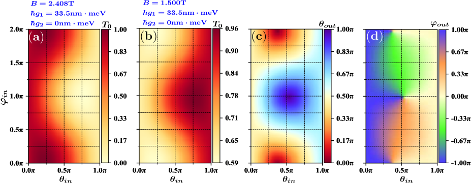
Figure 2: (color online). The energy of the incident electron is $E_{in}=198.5$ meV. (a) The total transmission rate $T_{0}$ for different angles of the polarization of the incident electron $(\theta_{in},\varphi_{in})$ when $\hbar g_{1}=33.5$ nm$\cdot$ meV and $g_{2}=0$ at $B=2.408$ T. (b) The total transmission rate $T_{0}$ and (c)-(d) the angles of the polarization of the outgoing electron $(\theta_{out},\varphi_{out})$ for different polarization of the incident electron $(\theta_{in},\varphi_{in})$ at $B=1.5$ T.

We suppose that the ring is only coupled by the Rashba spin-orbit interaction $\hbar g_{1}=20$ nm$\cdot$ meV and the incident current is already spin polarized. The polarization direction of the incident spin $(\theta_{in},\varphi_{in})$ varies and the charge transmission rate is indicated in Fig. 2. Fig. 2(a) shows the case when $T_{1}=1,T_{2}=0$ and $P_{0}=1$. The one-dimensional analytical model predicts that the outcoming polarization is along the eigenstate $\chi^{1}(0)$, $(0.161\pi,\pi)$, and the $\chi^{2}$ channel is closed $T_{2}=0$. In the two-dimensional model, it indicates that the outcoming polarization is along $(\theta_{out},\varphi_{out})=(0.214\pi,0.984\pi)$ always, where the channel of $\chi^{1}$ is free to transport and the other channel ($\chi^{2}$) is completely closed. It means that the polarization angle of the eigenstate of the 2D ring at $\varphi=0$ is $(0.214\pi,0.984\pi)$. This difference comes from the Zeeman effect and the finite width. It implies that these effects can also generate a finite $P_{y}$ in the ring with the Rashba SOC only, which is significantly differenti from the 1D model.

Moreover, the incident polarization with the maximum transmission rate among all the directions in the spin space is also along the eigenstate $\chi^{1}_{2D}(\pi)$, $(\theta_{in}^{max},\varphi_{in}^{max})=(0.214\pi,0.016\pi)$. We note that $(\theta_{in}^{max},\varphi_{in}^{max})$ and $(\theta_{out},\varphi_{out})$ are mirror symmetry to the $z$ axis.

The transmission of the spin-polarized input current in arbitrary direction is determined by the projection of $(\theta_{in},\varphi_{in})$ to $(\theta_{in}^{max},\varphi_{in}^{max})$, since the channel of $\chi^{2}_{2D}$ is closed. For a more general case, both transport channels of the eigensates allow electrons to pass ($T_{0}^{\max},T_{0}^{\min}>0$), as shown in Figs. 2(b) and (c), the maximum transmission rate $T_{0}^{\max}=0.962$ corresponds to the incident polarization $(\theta_{in}^{max},\varphi_{in}^{max})=(0.792\pi,0.963\pi)$, and its output polarization is $(\theta_{out}^{max},\varphi_{out}^{max})=(0.792\pi,0.037\pi)$. For the minimum transmission rate, we have $T_{0}^{\min}=0.591$, $(\theta_{in}^{\min},\varphi_{in}^{\min})=(0.208\pi,1.963\pi)$, $(\theta_{out}^{\min},\varphi_{out}^{\min})=(0.792\pi,1.037\pi)$. In this case, $(\theta_{out},\varphi_{out})$ is no longer a fixed angle along $\chi^{1}_{2D}$, but changes with the angle of incidence $(\theta_{in},\varphi_{in})$.

Interestingly, we also find numerically that the general relation between the incident angle and the charge transmission rates $T_{0}$ is given by

$$T_{0}=T_{0}^{\max}\cos^{2}\left(\frac{\theta_{\Delta}}{2}\right)+T_{0}^{\min}\sin^{2}\left(\frac{\theta_{\Delta}}{2}\right),$$ (8)

where $\theta_{\Delta}$ is the angle between the incident spin polarization $(\theta_{in},\varphi_{in})$ and the special angle $(\theta_{in}^{max},\varphi_{in}^{max})$, whether the outcoming spin is polarized or not. This equation is exactly the same as Eq. (3) that we found for the 1D model. The only difference is that in Eq. (3), $T_{1,2}$ correspond to the transmission rate of the eigenstates of the ring $\chi^{1,2}$. However, in the 2D ring the $T_{0}^{max}$ and $T_{0}^{min}$ correspond to the eigenstates of the 2D ring which are a little different from those of the 1D ring. The arbitrary spin is projected to the angles of the eigenstates of the ring, $(\theta_{in}^{max},\varphi_{in}^{max})$ and $(\pi-\theta_{in}^{max},\varphi_{in}^{max}+\pi)$. This projection then gives directly the transmission rate in Eqs. (3) and (8). The Zeeman coupling, circle symmetry breaking, and finite width only change the spin-polarization direction of eigenstates $\chi^{\mu}$, the properties predicted by the 1D analytical model are retained, which implies that we could use the quantum ring to design the integrable spin devices.

IV.2 Design of a spin analyzer

The ring acts as a spin torque: it allows the electron to pass but the spin polarization must be torqued. If the ring is coupled by the Dresselhaus spin-orbit interaction only, the similar spin torque occurs. The only difference is the outcoming angle of the spin, which is the mirror symmetry of the incident angle (for the maximum transmission rate only) to the plane $xOz$. The direction dependent transmission rate is also given by Eqs. (3) and (8).

According to the property of the angle dependent transmission rate in Eq. (8), we can realize a spin analyzer in the ring device. Before the measurement, we need to know $T_{0}^{max}$ and $T_{0}^{min}$ in a given magnetic field. They can be determined by the measurement of the transmission rates of the known spin polarized incidents. We use three spin polarized incident with $P_{x,y,z}=1$, respectively, and one spin unpolarized incident to identify the following parameters: $T_{0}^{max},T_{0}^{min},\theta_{in}^{max},\varphi_{in}^{max}$. The transmission rate for the unpolarized incident is marked as $T$, and we have already known $T=T_{0}^{max}+T_{0}^{min}$. The three transmission rates for different spin polarization incident are marked as $T(x),T(y)$ and $T(z)$. Applying Eq. (8) to $T(x),T(y)$ and $T(z)$, we find another three equations. So four equations in all can be solved and the four variables $T_{0}^{max},T_{0}^{min},\theta_{in}^{max},\varphi_{in}^{max}$ are found.

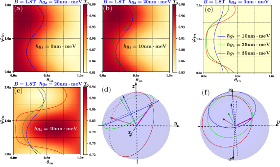
Figure 3: (color online). The energy of the incident electron is $E_{in}=198.5$ meV, and the background magnetic field $B=1.8$ T. (a)-(d) The colors represent the transmission rates for the SOCs $\hbar(g_{1},g_{2})=(0,20),(10,20),(40,20)$ nm$\cdot$ meV, respectively. The solid curve in (a) - (d) represents the possible angles of the incident polarization after the first, second and the third measurements, respectively. The dash lines in (b) and (c) represents the previous measurements. (d) The possible polarization is a cone for each measurement in the spin space. The blue, green and red arrows stand for the vector $(\theta^{max}_{in},\varphi^{max}_{in})_{1,2,3}$, respectively. The intersection of the three cones is the purple vector representing the incident polarization. (e)-(f) The intersections of the possible angles in three Rashba SOCs $\hbar g_{1}=10,25,35$ nm$\cdot$ meV, respectively, when the Dresselhaus is absent.

The scenario to analyze the spin polarization by detecting the charge transmission rates for different SOCs then can be established. The scheme is described as follows:

First, the ring is coupled by the two spin-orbit interactions $(g_{1},g_{2})$. The transmission rates are shown in colors in Fig. 3(a). $T_{0}^{max}$ and the corresponding incident polarization $(\theta_{in}^{max},\varphi_{in}^{max})_{1}$ is already known, as the blue vector in Fig. 3(d). Once we measure the transmission rate $T_{0}$, we can find the angle $\theta_{\Delta 1}$ between the incident polarization angle $(\theta_{in},\varphi_{in})$ and $(\theta_{in}^{max},\varphi_{in}^{max})_{1}$ by applying Eq. (8). However, the possible polarization direction in the three-dimensional space of the spin can be along any element of the cone, shown as the blue circle in Fig. 3(d). we project the angles of the elements of the cone onto the $(\theta,\varphi)$ plane to obtain the solid line in Fig. 3(a).

Second, we tune the Rashba SOC and the transmission rates are shown in colors in Figs. 3(b). The angle of the maximum transmission rate, $(\theta_{in}^{max},\varphi_{in}^{max})_{2}$, is represented by the green vector in Fig. 3(d). Then measure the transmission rate to obtain the angle $\theta_{\Delta 2}$ to find the second cone. The spin polarization is possibly located in the solid green line in Fig. 3(b), where the dashed line represents the first measurement. So the incident polarization must be at one of the intersection points of the two lines.

Thirdly, we tune the Rashba SOC again to find the third line which is shown in Fig. 3(c). The three lines must intersect at the same point which is the unique direction of the polarization of the incident spin. The intersection point can also be seen in the spin space in Fig. 3(d).

Here the external magnetic field is fixed and can be integrated on the chip. In fact, the three curves in the $(\theta,\varphi)$ plane always intersect at the same point for any magnetic field. A proper magnetic field results in better discrimination.

We note that the spin analyzer could be also achieved by a single SOC. In the 1D model, a single SOC only twists the spin in one direction ($x$ or $y$). The incident angle can not be uniquely determined, there are always two intersection points, no matter how many times we tune the strength of the SOC. However, in the real 2D ring, the spin can be twisted more widely. The unique intersection can appear. We show the numerical results in Fig. 3(e) where only the Rashba SOC exists and the Dresselhaus SOC is absent. It is clear that after three measurements with different strengthes of the Rashba SOC, all the cones intersect at the unique intersection and the other intersection has been lifted. So the spin polarization can also be identified more easily.

V Conclusion

In summary, we present a detailed study of the transport properties of the device in which a quantum ring is in contact with two leads at the ends of one diameter. When the SOC is introduced, different phases are added in the matter wave of the electron with different spins. So that the transmission rates for different spins are no longer degenerate. By detailed analytical and numerical studies, we find that in a simple quantum ring device, the spin unpolarized current can be spin polarized parallel to the eigenstates of the ring for appropriate SOC and the magnetic field. The direction of the polarization can be tuned easily by the SOC and the magnetic field as well. This simple device is therefore proposed to be a spin polarizer. Moreover, similar to the light polarizer/analyzer, it can also be designed as an omnidirectional all-electric spin analyzer by simply measuring the transmission rate of the polarized incident via Eq. (8). These findings pave the way to control the system in spintronics and may be useful in quantum computation. It also contributes an easy and controllable proposal to the design of the high-performance all-electric transport device.

VI Acknowledgement

This work is supported by the NSF-China under Grant No. 11804396. J.S. is supported by the NSF-China under Grant No. 11804397. A.G. acknowledges financial support by the NSF-China under Grant No. 11874428, 11504066, and the Innovation-Driven Project of Central South University (CSU) (Grant No. 2018CX044). F.O. acknowledges financial support by the NSF-China under Grant No. 51272291, the Distinguished Young Scholar Foundation of Hunan Province (Grant No. 2015JJ1020), and the CSU Research Fund for Sheng-hua scholars (Grant No. 502033019). T.C. would like to thank Junsaku Nitta for helpful discussion, in particular, for pointing out Ref. Hatano .

Appendix A Method and Formalism

Here we explicitly derive the transmission rate in Eq. (1). We consider electrons as plane waves in the two leads with momentum $\hbar k$ and energy $E=\frac{\hbar^{2}k^{2}}{2m^{\ast}}$. Note that there is an additional potential $U_{0}=-\beta_{1}^{2}$ induced by the Rashba SOC sheng , so that in the two arms, $E=\frac{\hbar^{2}k_{0}^{2}}{2m^{\ast}}+U_{0}$. The wave vector in the two arms are AC3 $k_{j}^{\mu}=k_{0}+j\left(\frac{\Phi_{AB}}{2\pi r_{0}}+\frac{\Phi_{AC}^{\mu}}{2\pi r_{0}}\right).$ The incident current can be decomposed into the two eigenstates $\chi^{1,2}$, and the electron is transported by this two channels. We note that in this case the two channels are independent and there is no interference between the two eigenstates. If the incident spin is polarized along $\chi^{\mu}$ then the outcoming polarization is still along $\chi^{\mu}$. If the incident current is decomposed into other two orthogonal states, then the interference is difficult to deal with.

The wave function at the left lead contains the incident and the reflection, $\Psi_{in}^{\mu}$. The wave function of the upper arm also contains two parts, the clockwise and the anticlockwise movements, $\Psi_{1}^{\mu}$. In the same manner, the wave function of the lower arm is $\Psi_{2}^{\mu}$. The output wave function is marked $\Psi_{out}^{\mu}$. All these wave functions are given by

$$\Psi_{in}^{\mu} = \left(e^{ikx}+r^{\mu}e^{-ikx}\right)\chi^{\mu}\left(\pi\right),$$ (S1)

$$\Psi_{1}^{\mu} = \sum_{j}C_{j}e^{jik_{j}^{\mu}x}\chi^{\mu}\left(\phi\right),$$ (S2)

$$\Psi_{2}^{\mu} = \sum_{j}D_{j}e^{jik_{-j}^{\mu}x}\chi^{\mu}\left(\phi\right),$$ (S3)

$$\Psi_{out}^{\mu} = t_{\mu}e^{ikx}\chi^{\mu}\left(0\right),$$ (S4)

where $r^{\mu}$ is the reflection rate, $C,D$ are the parameters which can be determined by the continuous condition, and $t_{\mu}$ is the variable characterizing the transport properties of the device. The transmission rate is thus given by $T_{\mu}=|t_{\mu}|^{2}$. By applying the Griffith boundary conditions Griffith ; AC1 ; Bellucci ; Citro ; Tang ; Saeedia ; Zhai , the wave functions and the currents must be continuous at the two leads ($x=\pm r_{0}$ or $\theta=0,\pi$), we obtain six equations to solve the six variables. Among them, the most wanted transmission rate can be solved,

$$T_{\mu}=\frac{K\Phi^{\mu}}{KK^{\prime}+\left[4k_{0}^{2}\left(\Phi^{\mu}-K^{\prime}\right)+k^{2}\sin^{2}(\pi k_{0}r_{0})\right]^{2}},$$ (S5)

which is shown as Eq. (1).

In order to calculate the transport properties numerically, it is convenient to discretize the continuous Hamiltonian. We discretize $H$ on the sites of a square lattice with the lattice constant $a$ to obtain the tight binding Hamiltonian. It is obtained by calculating the matrix elements in the basis of position. The tight binding Hamiltonian is given by

$$H =\sum\limits_{i}\left(V_{i}+4t+\frac{\Delta}{2}\sigma_{z}\right)c_{i}^{\dagger}c_{i}-\sum_{\left\langle i,j\right\rangle}\left(t+s_{ij}\right)c_{i}^{\dagger}c_{j}e^{i\theta_{ij}},$$ (S6)

$$t =\frac{\hbar^{2}}{2m^{\ast}a^{2}},$$ (S7)

$$s_{ij} =-\frac{i\hbar g_{1}}{2a^{2}}\left(\sigma_{x}\Delta y-\sigma_{y}\Delta x\right)-\frac{i\hbar g_{2}}{2a^{2}}\left(\sigma_{y}\Delta y-\sigma_{x}\Delta x\right),$$ (S8)

$$\theta_{ij} =\frac{e}{\hbar}\left(A_{x_{i}}\Delta x+A_{y_{i}}\Delta y\right),$$ (S9)

where $i$ runs over all sites, $\left\langle i,j\right\rangle$ represents the nearest neighbouring hopping only, $x_{i}$ and $y_{i}$ are the $x$ and $y$ coordinates of site $i$, and $\Delta x_{ij}=x_{j}-x_{i}$, $\Delta y_{ij}=y_{j}-y_{i}$. For convenience, we apply a hard-wall potential instead of the parabolic potential,

$$V_{i}=\begin{cases}0&\left|r_{i}-r_{0}\right|\leqslant r_{w}\\ \infty&\left|r_{i}-r_{0}\right|>r_{w}\end{cases},$$ (S10)

where $r_{i}=\sqrt{x_{i}^{2}+y_{i}^{2}}$ and the width of the ring is $r_{w}$. We connect two parallel leads to the ring, then the transmission properties can be obtained by using the nonequilibrium Green’s function (NEGF).

It is worthwhile to note that the continuous model and the tight binding model are compatible and all the observable quantities in these two models are almost equal (the small errors vanish when $a\rightarrow 0$). Moreover, the energy spectrum has no essential difference in a parabolic potential from that in a hard-wall potential, if $r_{w}$ matches the confinement $\hbar\omega$. Then we consider the transport properties in such a lattice model with tight-binding Hamiltonian. The spin transmission rate $T$ of the electron transporting from the left lead to the right lead is defined by using the NEGF method dattabook ; chang ,

$$T_{\alpha}(E)=\text{Tr}\{\sigma_{\alpha}[\Gamma_{R}(E)G_{RL}(E)\Gamma_{L}(E)G_{LR}^{{\dagger}}(E)]\},$$ (S11)

where $\alpha\in\left\{x,y,z\right\}$, $\sigma_{x,y,z}$ are the Pauli matrices and $\sigma_{0}$ is the unit matrix. The Green’s function is defined by the projection of the full Green’s function dattabook ,

$$G_{RL} = P_{R}GP_{L},$$ (S12)

$$G(E) = (E-H-\Sigma_{R}-\Sigma_{L})^{-1},$$ (S13)

where $P_{R},P_{L}$ are the projection operators to the right and the left leads, $\Sigma_{R},\Sigma_{L}$ are the self-energy of the right and the left leads, respectively. The broadening function is defined by $\Gamma_{j}=i\left[\Sigma_{j}-\Sigma_{j}^{\dagger}\right]$.

$T_{\alpha}(E)$ is the transmission rate of the $\left(\alpha\in\left\{x,y,z\right\}\right)$ component of the spin or the total charge transmission $\left(\alpha=0\right)$ while the energy of the incident electron is $E$. Then the spin polarization rate $P$ is defined as:

$$P_{{}_{\alpha}}=\frac{T_{\alpha}}{T_{0}}\times 100\%,\alpha\in\left\{x,y,z\right\}$$ (S14)

and $P_{0}=\sqrt{T_{x}^{2}+T_{y}^{2}+T_{z}^{2}}/T_{0}=\sqrt{P_{x}^{2}+P_{y}^{2}+P_{z}^{2}}$. $P_{0}$ represents the spin polarization of the outcoming electron. If $P_{0}=1$, then the spin is fully polarized. If $P_{0}=0$, the spin is fully unpolarized.

By diagonalizing the tight-binding Hamiltonian in Eq. (S6), we can have the value of the wave functions at each site, $\psi\left(\mathbf{r}_{i}\right)$, which is a two component spinor. The physical quantities can then be obtained. The spin fields are calculated by

$$\sigma_{\alpha}\left(\mathbf{r}_{i}\right)=\psi^{{\dagger}}\left(\mathbf{r}_{i}\right)\sigma_{\alpha}\psi\left(\mathbf{r}_{i}\right),$$ (S15)

and the density is given by $n\left(\mathbf{r}_{i}\right)=\psi^{{\dagger}}\left(\mathbf{r}_{i}\right)\psi\left(\mathbf{r}_{i}\right)$. The average value of the observable quantity is thus given by $\left\langle A\right\rangle=\sum_{i}\psi^{{\dagger}}\left(\mathbf{r}_{i}\right)A\psi^{{\dagger}}\left(\mathbf{r}_{i}\right)\Delta x\Delta y$. The in-plane field can be described by the vector field $\bm{\sigma}\left(\mathbf{r}\right)=\left(\sigma_{x}\left(\mathbf{r}\right),\sigma_{y}\left(\mathbf{r}\right)\right).$

The current operators can be derived by $j_{\mu}=-\frac{\delta H}{\delta A}$, so that the on-site current densities are given by

$$j_{x}\left(\mathbf{r}_{i}\right) =\frac{e}{2m^{\ast}}\left[\psi^{{\dagger}}\left(\mathbf{r}_{i}\right)P_{x}\psi\left(\mathbf{r}_{i}\right)+\left(P_{x}\psi\left(\mathbf{r}_{i}\right)\right)^{{\dagger}}\psi\left(\mathbf{r}_{i}\right)\right]$$

$$-e\psi^{{\dagger}}\left(\mathbf{r}_{i}\right)\left(g_{1}\sigma_{y}+g_{2}\sigma_{x}\right)\psi\left(\mathbf{r}_{i}\right),$$ (S16)

$$j_{y}\left(\mathbf{r}_{i}\right) =\frac{e}{2m^{\ast}}\left[\psi^{{\dagger}}\left(\mathbf{r}_{i}\right)P_{y}\psi\left(\mathbf{r}_{i}\right)+\left(P_{y}\psi\left(\mathbf{r}_{i}\right)\right)^{{\dagger}}\psi\left(\mathbf{r}_{i}\right)\right]$$

$$+e\psi^{{\dagger}}\left(\mathbf{r}_{i}\right)\left(g_{1}\sigma_{x}+g_{2}\sigma_{y}\right)\psi\left(\mathbf{r}_{i}\right).$$ (S17)

The current is contributed by three parts,

$$j_{\alpha}\left(\mathbf{r}_{i}\right)\equiv j_{z\uparrow,\alpha}\left(\mathbf{r}\right)+j_{z\downarrow,\alpha}\left(\mathbf{r}\right)+j_{SOC,\alpha}\left(\mathbf{r}\right),$$ (S18)

where

$$j_{z\uparrow,\alpha}\left(\mathbf{r}_{i}\right) = \frac{e}{2m^{\ast}}\left[\psi_{\uparrow}^{*}P_{\alpha}\psi_{\uparrow}+\left(P_{\alpha}\psi_{\uparrow}\right)^{*}\psi_{\uparrow}\right],$$ (S19)

$$j_{z\downarrow,\alpha}\left(\mathbf{r}_{i}\right) = \frac{e}{2m^{\ast}}\left[\psi_{\downarrow}^{*}P_{\alpha}\psi_{\downarrow}+\left(P_{\alpha}\psi_{\downarrow}\right)^{*}\psi_{\downarrow}\right],$$ (S20)

$$j_{SOC,x}\left(\mathbf{r}_{i}\right) = -e\psi^{{\dagger}}\left(g_{1}\sigma_{y}+g_{2}\sigma_{x}\right)\psi,$$ (S21)

$$j_{SOC,y}\left(\mathbf{r}_{i}\right) = e\psi^{{\dagger}}\left(g_{1}\sigma_{x}+g_{2}\sigma_{y}\right)\psi.$$ (S22)

The on-site wave function spinor is $\psi=\left(\begin{array}[]{cc}\psi_{\uparrow}&\psi_{\downarrow}\\ \end{array}\right)^{T}$, and $\uparrow,\downarrow$ are related to the eigenstates of the spin operator $\sigma_{z}$.

Appendix B Spin transmissions in different SOCs – Spin filtering and spin polarizer

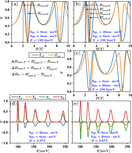
Figure S1: (color online). $T_{z\uparrow}$ and $T_{z\downarrow}$ (a) without SOC, (b) with the Rashba SOC only, and (c) with the Dresselhauss SOC only. $T_{\alpha}$ $\alpha\in\left(x,y,z\right)$ (d) with the Rashba SOC only and (e) with the Dresselhauss SOC only.

We study in details how the transmission rate is related to the magnetic field and the SOCs. We suppose that the input electrons are spin unpolarized. If there is no SOC, the transported electrons are spin unpolarized as well, i.e., $T_{z\uparrow}=T_{z\downarrow}$ for $g=0$. However, the Zeeman coupling makes the transmission rate different, especially in a strong magnetic field, as shown in Fig. S1(a). Since the minimum transmission rates for spin up and down are all located at the same magnetic field, it would be difficult to suppress one spin to zero and keep the other spin finite.

If the SOCs are introduced into the system, we find that the transmission rate curves for spin down and spin up are well separated. If only the Rashba SOC is present, the curve of $T_{z\downarrow}$ is shifted left and the curve of $T_{z\uparrow}$ is shifted right as shown in Fig. S1(b). If only the Dresselhaus SOC exists, the shift of the curves is just opposite to that in a Rashba ring, as shown in Fig. S1(c).

If there is no magnetic field, the electron transports through the upper arm and the lower arm with the same phase added ($T_{1}=T_{2}$), so that the transmission rates for different spins depend on the ring itself and are equal, as shown in Figs. S1(b) and (c). However, in finite magnetic fields the time-reversal symmetry is broken, the spin degeneracy in the ring will be lifted more in the presence of either Rashba or Dresselhas SOC strongly. Such a combination of the magnetic field and the SOCs can lead to significant spin filtering effect.

In the numerical curves (Figs. S1(b) and (c)), the spin filtering appears periodically in a magnetic field, since the term $\Phi_{AB}+\Phi_{AC}$ in transmission rate Eq. (1) only depends on the magnetic field. For instance, if only the Rashba SOC is present and the energy of the incident electron is $E_{in}=198.5$ meV in Fig. S1(b), the lowest magnetic field where the spin down is suppressed is at $B=2.67$T, which can be further lowered by increasing the radius of the ring (at the same magnetic flux). In this case, $T_{z\downarrow}\rightarrow 0$ and $T_{z\uparrow}$ is finite, so that the output electrons are almost polarized to spin up, $P_{z}\rightarrow 1$. For different energies of the input electrons, the transmission rates are shown in Figs. S1(d) and (e). The negative $T_{i}$ represents the $i$ component of the output spin is polarized in the negative direction of the $i$ axis. In fact, according to Fig. S1(d) and the analysis of the 1D model, the output spin is polarized along $\chi^{1,2}$ between the $z$ and $-x$ axis, since $T_{y}\approx 0$ and $T_{x,z}$ are finite.

We now compare the transmission curves of the ring without SOC (Fig. S1(a)) and the ring with Rashba SOC (Fig. S1(b)). The first maximum rate for $T_{z\uparrow}$ is at $B_{maxT}$ in the ring without SOC. After the Rashba SOC is set in, both of the $T_{z\uparrow}$ and $T_{z\downarrow}$ transmission rates are shifted. We suppose that the first maximum value of $T_{z\uparrow}$ is shifted to $B^{\prime}_{maxT}$. In the same manner, the first minimum rate in the ring without SOC is at $B_{minT}=2.83$T, while the first minimum rate $T_{z\downarrow}$ is shifted to $B^{\prime}_{minT}$. We define the parameters $\Delta B_{maxT}=B^{\prime}_{maxT}-B_{maxT}$, $\Delta B_{minT}=B_{minT}-B^{\prime}_{minT}$, and $\Delta B_{T}=B^{\prime}_{minT}-B^{\prime}_{maxT}$ to study how the Rashba SOC shifts the transmission rate curve and changes the polarization of the spin.

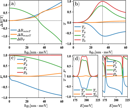
Figure S2: (color online). (a) Magnetic field shifts $\Delta B$ induced by the Rashba SOC. (b) Spin transmission rates $T$ and (c) spin polarization $P$ in different $g_{1}$ with incident electron energy $198.5$ meV, in the magnetic field where the minimum $T_{z\downarrow}$ is, so that $P_{0}=1$ always. (d) The spin transmission rate $T$ and (e) the spin polarization $P$ at $\hbar g_{1}$ = 33.5 nm$\cdot$meV and $B$=2.41 T (corresponding to $\Delta B_{T}=0$) with energy.

We show that in Fig. S2(a) $\Delta B_{T}$ decreases with the increase of the Rashba SOC $g_{1}$, due to the change of the AC phase $\Phi_{AC}^{\mu}$, just as predicted in the 1D model. When $\hbar g_{1}=33.5$ nm$\cdot$ meV, $\Delta B_{T}=0$, which means that the transmission rate of spin down is suppressed to minimum and the transmission rate of spin up is maximum. Interestingly, at this point the total charge transmission rate is exactly $1$ as shown in Fig. S2(b). Hence, $\chi^{1}$ is completely suppressed, and $\chi^{2}$ passes the ring freely. Meanwhile, the $y$ component of the spin is almost suppressed, $T_{y}\approx 0$, and both $|T_{x}|$ and $|P_{x}|$ increase, as shown in Figs. S2(b) and (c). We are then able to control the direction of the spin polarization by tuning the Rashba SOC. The tunable spin polarizer is thereby established. In Fig. S2(d), we show how the spin polarization and the transmission rate vary with the energy of the incident electron. Basically, $T_{y}$ is close to 0 and $P_{y}$ is also always very small. It is nonzero comparing with the 1D model, due to the Zeeman coupling and the width of the ring. In Figs. S2(d) and (e) we show that if the energies of the incident electrons are in the region $[185,205]$ meV, the spin transmission and polarization are stable. So that the outcoming current which is obtained by integral of the transmission rate $T$ over this region is almost fully spin polarized. In order to exclude the unwanted transmission below $185$meV, we can apply a gate to lift the whole energy band of the lead.

In our ring device, the Rashba SOC tilts the spin to the $x$ axis, while the Dresselhaus SOC flip the spin towards the $y$ direction. It can also be understood simply as follows. When the magnetic field is absent, the effective vector potential induced by the SOCs is

$$A_{x}^{SOC} = -\frac{m}{e\hbar}(g_{1}\sigma_{y}+g_{2}\sigma_{x}),$$ (S23)

$$A_{y}^{SOC} = \frac{m}{e\hbar}(g_{1}\sigma_{x}+g_{2}\sigma_{y}).$$ (S24)

Suppose the incident wave function is spin polarized, $\psi^{in}_{+}=(\begin{array}[]{cc}1&0\end{array})^{T}$, then the outcoming wave function influenced by the SOC is given by $\psi^{out}\propto e^{-iA_{x}\cdot 2(r_{0}+r_{w})}\psi^{in}$, since the coordinate difference in the $y$ direction is zero. If there is only Rashba existing,

$$\psi^{out}_{R}\propto(1+i\gamma g_{1}\sigma_{y})\left(\begin{array}[]{c}1\\ 0\\ \end{array}\right)=\left(\begin{array}[]{c}1\\ -\gamma\\ \end{array}\right),$$ (S25)

where $\gamma=2(r_{0}+r_{w})\frac{m}{e\hbar}g_{1}>0$. So we have $\langle\sigma_{x}\rangle=-2\gamma<0$ and $\langle\sigma_{y}\rangle=0$. The spin is torqued from the $+z$ direction to $-x$. If the incident electron is spin down, $\psi^{in}_{-}=(\begin{array}[]{cc}0&1\end{array})^{T}$, then $\psi^{out}_{R}=(\begin{array}[]{cc}\gamma&1\end{array})^{T}$, and then $\langle\sigma_{x}\rangle=2\gamma>0$ and $\langle\sigma_{y}\rangle=0$. In Fig. S2(d), however spin down is suppressed in the transport, and the spin up $\psi^{in}_{+}$ is flipped to the $-x$ axis. On the other hand, if only the Dresselhaus SOC is present, we can do the same calculation. For $\psi^{in}_{+}$, $\psi^{out}_{D}=(\begin{array}[]{cc}1&i\gamma\end{array})^{T}$, so that $\langle\sigma_{x}\rangle=0$ and $\langle\sigma_{y}\rangle=2\gamma>0$. For $\psi^{in}_{-}$, $\psi^{out}_{D}=(\begin{array}[]{cc}i\gamma&1\end{array})^{T}$, so that $\langle\sigma_{x}\rangle=0$ and $\langle\sigma_{y}\rangle=-2\gamma<0$. In Fig. S2(e), the spin up is suppressed, while the spin down $\psi^{in}_{-}$ is flipped to the $-y$ axis in the transport. The analysis agrees with the numerical results perfectly.

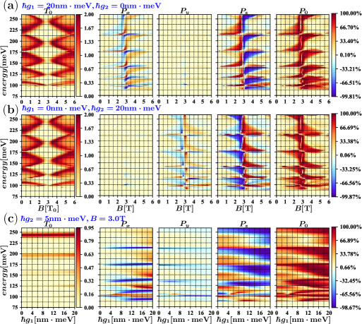
Figure S3: (color online). The transmission $T$ and spin polarizability $P$ with (a) Rashba SOC only, (b) Dresselhauss SOC only, and (d) fixed Dresselhauss SOC but tunable Rashba SOC.

As drawn in Fig. S3, we show the relation between the spin transmission rates and the spin polarizations for different SOCs. If only the Rashba SOC is existing, then $T_{y}$ and $P_{y}$ will be suppressed shown in Fig. S3(a). The direction of the spin polarizer can be tuned by the strength of the Rashba SOC in the plane $xOz$. If only the Dresselhaus SOC is present, then $T_{x}$ and $P_{x}$ will be suppressed shown in Fig. S3(b). The direction of the spin polarizer is then in the plane $yOz$. If both of the SOCs are present, then the situation becomes complicated and spin polarizer can be controled more widely, as shown in Fig. S3(c). However, we find that if the outcoming spin needs to be polarized well, then it is better to keep one SOC dominating the system. The competition of the two SOCs makes the spin more difficult to be polarized.

Appendix C Spin textures and current in the transport

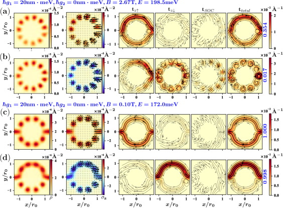
Figure S4: (color online). Transport status and transmission flow density for electrons with fixed incident energy and magnetic fields in a Rashba ring. The first two columns (from left to right) show the charge and spin fields when the transport reaches the equilibrium status, the colors represent the density and $\sigma_{z}(\mathbf{r})$, respectively. In (a) and (b), strong spin filtering is found, i.e. the transmission rate of spin up is much higher than that of spin down. In (c) and (d) the outcoming spin is fully unpolarized although the total transmission rate is almost 1. For (a) and (b), $\hbar g_{1}=20$ nm$\cdot$ meV, $B=2.67$ T and the incident energy is $198.5$ meV. For (c) and (d), $\hbar g_{1}=20$ nm$\cdot$ meV, $B=0.1$ T and the incident energy is $172$ meV.

The incident spin is supposed to be unpolarized, so that the wave function of the incident electrons $\psi^{in}$ can be decomposed to two parts in any direction of the spin polarization. Without the loss of generality, we decompose the incident electron in the basis of $\sigma_{z}$, $|\psi^{in}_{z\uparrow}|^{2}=|\psi^{in}_{z\downarrow}|^{2}$. The spins of the two parts are independently polarized along $z$ or $-z$ direction, respectively. For each part of the incident electron, it contributes one transmission channel in the transport. Then we can figure out which channel plays more important role in the transport. The wave function of the incident electron is supposed to be the wave function of the lowest band of the lead. By employing Eq. (7) we can obtain the wave function in the ring by the Green’s function method,

$$\psi^{ring}=G\tau_{L}\psi^{in}_{z\uparrow(\downarrow)},$$ (S26)

where $\tau_{L}$ is the coupling matrix between the incident (left) lead and the ring dattabook . We again employ the current densities $\mathbf{j}_{z\uparrow},\mathbf{j}_{z\downarrow}$ and $\mathbf{j}_{SOC}$ defined in Eqs. (S19) to (S22), where $\psi$ needs to be replaced by $\psi^{ring}$. We can define the transmission density $t_{\alpha}(\mathbf{r})$ proportional to the current,

$$t_{\alpha}(\mathbf{r})=-\frac{\hbar}{2e\cdot\text{meV}}\mathbf{j}_{\alpha}(\mathbf{r}).$$ (S27)

The transmission rate is thus obtained by $T_{\alpha}=\sum_{i}t_{\alpha}(\mathbf{r}_{i})$, where $i$ includes all the sites between the lead and the ring.

For simplicity, we consider only the Rashba SOC in two different cases: (i) $\hbar g_{1}=20$ nm$\cdot$ meV at $B=2.76$T, the electron of the incident energy $E_{in}=198.5$ meV has the transmission rate $T_{0}=0.372$; (ii) $\hbar g_{1}=20$ nm$\cdot$ meV at $B=0.1$T, the transmission rate of the electron with $E_{in}=172$ meV is $T_{0}=1.998$. In Figs. S4(a) and (b), we show how the incident wave functions $\psi^{in}_{z\uparrow}=(\begin{array}[]{cc}1&0\end{array})^{T}$ and $\psi^{in}_{z\downarrow}=(\begin{array}[]{cc}0&1\end{array})^{T}$ are transported through the ring, respectively, where the outcoming spin is polarized and the transport rate is relatively low. In Figs. S4(c) and (d), we show how the incident wave functions transport in the ring when the magnetic field is $B=0.1$T, where the electrons pass through the ring freely but the spin is not polarized at all.

When the transport reaches the equilibrium status, the spin and charge densities and the current densities are plotted in Fig. S4. Both the charge densities and the spin textures shown in the first two columns (from left to right) of Fig. S4 are periodically distributed in the ring as a stationary wave, due to the interference of the matter wave of the electron. The spin textures also support the analysis of the outcoming spins derived in Eq. (S25), i.e. at the right lead $\langle\sigma_{y}\rangle=0$, the $x$ component spin is generated in the transport by the SOC and the direction of $\sigma_{x}(r)$ depends on the polarization of the incident spin.

Comparing with the case without the magnetic field sun ; datta , here the vector potential of the external magnetic field and the effective vector potential induced by the SOC give different phases to the upper and the lower arms, respectively. This phase difference leads to different transmission for different spins and can be observed by the transport experiment.

In the spin up channel in case (i), electron is mostly transported by the current $\mathbf{j}_{z\uparrow}$, which means the SOC does not contribute a lot in the transmission. In the spin down channel, the SOC flips spin and induces stronger transmission. However, the transmission of this channel is still weak, only contributes $1/20$ of the spin up channel. In this case, the spin is thus strongly polarized. In the case (ii), both of the two channels have high transmission rate, close to $1$. The current in the spin down channel is obviously imbalanced in the upper and lower arms. However the outcoming spin has half in spin up and half in spin down, which means that the ring in this case is good in transport but fails to polarize the spin.

There are circular currents in the ring, which do not contribute to total transmission, when the transmission rate is low. It keeps the current conserved. If the transmission is high, the internal circling is weak, but the imbalance between the currents of the upper and the lower arms is explicit. From the detailed transport pictures shown in Fig. S4, we can clearly see how the electron passes through the ring. This method is general and can be applied to other systems as well.

References

- (1) T. Chakraborty, A. Manaselyan, and M. Berseghyan, in Physics of Quantum Rings (Springer, Berlin 2018), edited by V.M. Fomin.
- (2) T. Chakraborty, and P. Pietiläinen, Phys. Rev. B 52, 1932 (1995); Hong-Yi Chen, P. Pietiläinen, and Tapash Chakraborty, Phys. Rev. B 78, 073407 (2008).
- (3) S. Datta and B. Das, Appl. Phys. Lett. 56, 665 (1990).
- (4) Qing-feng Sun, and X. C. Xie, Phys. Rev. B 71, 155321 (2005).
- (5) Feng Chi, Lian-Liang Sun, Ling Huang and Jia Zhao, Chin. Phys. B, 20, 017303 (2011).
- (6) P.H. Chang, F. Mahfouzi, N. Nagaosa, and Branislav K. Nikolić, Phys. Rev. B, 89, 195418 (2014).
- (7) Moumita Dey, Santanu K. Maiti, Sreekantha Sil and S. N. Karmakar, Journal of Applied Physics 114, 164318 (2013).
- (8) Pojen Chuang, Sheng-Chin Ho, L. W. Smith, F. Sfigakis, M. Pepper, Chin-Hung Chen, Ju-Chun Fan, J. P. Griffiths, I. Farrer, H. E. Beere, G. A. C. Jones, D. A. Ritchie and T.-M. Chen, Nat. Nanotechnol. 10, 35 - 39 (2015).
- (9) Miao Wang and Kai Chang, Phys. Rev. B 77, 125330 (2008).
- (10) Shreekantha Sil, Santanu K. Maiti, and Arunava Chakrabarti, J. Appl. Phys. 112, 024321 (2012).
- (11) J. Nitta, F. E. Meijer, H. Takayanagi, Appl. Phys. Lett. 75, 695 (1999).
- (12) T. Choi, S. Y. Cho, C. M. Ryu, and C. K. Kim, Phys. Rev. B 56, 4825 (1997).
- (13) C. M. Ryu, T. Choi, C. K. Kim, and K. Nahm, Mod. Phys. Lett. B 10, 401 (1996).
- (14) S. Gumber, A B. Bhattacherjee, P K. Jha, Phys. Rev. B 98, 205408 (2018).
- (15) B. Molnár, F. M. Peeters, and P. Vasilopoulos, Phys. Rev. B 69, 155335 (2004).
- (16) D. Frustaglia and K. Richter, Phys. Rev. B 69, 235310 (2004).
- (17) P. Lucignano, D. Giuliano, and A. Tagliacozzo, Phys. Rev. B 76, 045324 (2007).
- (18) J. Wang, and K. S. Chan, J. Phys.: Condens. Matter 21, 245701 (2009).
- (19) H. Z. Tang, L. X. Zhai, M. Shen, J. J. Liu, Physics Letters A 378, 2790-2794 (2014).
- (20) S. Bellucci and P. Onorato, J. Phys.: Condens. Matter 19, 395020 (2007); Eur. Phys. J. B 73, 215 (2010).
- (21) R. Citro, F. Romeo, M. Marinaro, Phys. Rev. B 74, 115329 (2006).
- (22) V. M. Kovalev, A. V. Chaplik, Journal of Experimental and Theoretical Physics, 103, 781 (2006).
- (23) S. Saeedia and E. Faizabadi, Eur. Phys. J. B 89, 118 (2016).
- (24) L. X. Zhai, Y. Wang, Z. An, AIP Advances 8, 055120 (2018).
- (25) Qing-feng Sun, Jian Wang and Hong Guo, Phys. Rev. B 71, 165310 (2005).
- (26) S. Griffith, Trans. Faraday Soc. 49, 345 (1953).
- (27) C. Li, Y. J. Li, D. X. Yu, C. L. Jia, New J. Phys. 20, 093023 (2018).
- (28) N. Hatano, R. Shirasaki, and H. Nakamura, Phys. Rev. A 75, 032107 (2007).
- (29) A S. Naeimi, Eslami, M. Esmaeilzadeh, J. Appl. Phys. 113, 044316 (2013).
- (30) Evgeny Y. Tsymbal and Igor Z̆utić, Handbook of spin transport and magnetism, CRC Press, Boca Raton (2012).
- (31) Di-Jing Huang, Jae-Yong Lee, Jih-Shih Suen, G. A. Mulhollan, A. B. Andrews, and J. L. Erskine, Rev. Sci. Instrum. 64, 3474 (1993).
- (32) C. Jozwiak, J. Graf, G. Lebedev, N. Andresen, A. K. Schmid, A. V. Fedorov, F. El Gabaly, W. Wan, A. Lanzara, and Z. Hussain, Rev. Sci. Instrum. 81, 053904 (2010).
- (33) J. Nitta, T. Akazaki, H. Takayanagi, and T. Enoki, Phys. Rev. Lett. 78, 1335 (1997).
- (34) C. R. Ast, D. Pacilé, L. Moreschini, M. C. Falub, M. Papagno, K. Kern, M. Grioni, J. Henk, A. Ernst, S. Ostanin, and P. Bruno, Phys. Rev. B 77, 081407(R) (2008).
- (35) Y. Kanai, R. S. Deacon, S. Takahashi, A. Oiwa, K. Yoshida, K. Shibata, K. Hirakawa, Y. Tokura, and S. Tarucha, Nat. Nanotechnol. 6, 511 (2011).
- (36) M. P. Nowak, B. Szafran, F. M. Peeters, B. Partoens, and W. J. Pasek, Phys. Rev. B 83, 245324 (2011).
- (37) Shenglin Peng, Wenchen Luo, Fangping Ouyang, and Tapash Chakraborty, arXiv:1911.01613 (2019).
- (38) J. S. Sheng and Kai Chang, Phys. Rev. B 74, 235315 (2006).
- (39) S. Oh and C.-M. Ryu, Phys. Rev. B 51, 13441 (1995).
- (40) S.-Q. Shen, Z.-J. Li, Z.-S. Ma, Appl. Phys. Lett. 84, 996 (2004).
- (41) S. Datta, Quantum Transport: Atom to Transistor (Cambridge University Press, Cambridge, 2005).
- (42) The lattice constant of InAs is about nm, however, the results of nm lattice are no significantly different from the real physical system. For simplicity and saving computing resources we utlized a larger lattice constant.
- (43) T. Chakraborty, Quantum Dots (Elsevier, 1999).