Annular and circular rigid inclusions planted into a penny-shaped crack and factorization of triangular matrices

Abstract

Analytical solutions to two axisymmetric problems of a penny-shaped crack when an annulus-shaped (model 1) or a disc-shaped (model 2) rigid inclusion of arbitrary profile are embedded into the crack are derived. The problems are governed by integral equations with the Weber–Sonin kernel on two segments. By the Mellin convolution theorem the integral equations associated with the models 1 and 2 reduce to vector Riemann-Hilbert problems with $3\times 3$ and $2\times 2$ triangular matrix coefficients whose entries consist of meromorphic and of infinite indices exponential functions. Canonical matrices of factorization are derived and the partial indices are computed. Exact representation formulas for the normal stress, the stress intensity factor, and the normal displacement are obtained and the results of numerical tests are reported.

1 Introduction

Axisymmetric problems of the loading of penny-shaped cracks by normal tractions applied at the crack faces in a homogeneous or a composite unbounded elastic body have been examined by many researchers including [1], [2], [3], [4], [5], [6]. Relevance to modeling of hydraulically induced fracture of resource bearing geological formations was a motivation [7] for some of these studies. The model problems admit an exact solution by quadratures or in a series form by a variety of methods such as Abelian operators, the Wiener–Hopf technique, orthogonal polynomials, and the Radon transform. Motivated by modeling of fracture processes in composite elastic materials which are reinforced with dilute concentrations of rigid circular inclusions Selvadurai and Singh analyzed [7] the problem of indentation of a penny-shaped crack by a smooth disc-shaped rigid inclusion. They employed Sneddon’s integral representation [1] of the general solution of the axisymmetric biharmonic equation in terms of two arbitrary functions and then expressed the normal traction and displacement on the boundary of the upper half-space through a single function. By the method of Abelian operators the governing triple integral equation was reduced to a Fredholm integral equation of the second kind that was solved approximately by an asymptotic method. However, as it is shown in Section 2.1 of our paper, it is impossible to formulate the boundary conditions in terms of a single function. This means that the governing triple equations and the associated Fredholm equation are not equivalent to the model, and the asymptotic formula for the stress intensity factor is incorrect.

The goal of this paper is to derive an analytical solution to two problems of a penny shaped crack when an annular (model 1) or a circular inclusion (model 2) is embedded into the crack. The inclusions are assumed to be rigid and not necessary flat. We do not employ the theory of Abelian operators and do not end up with Fredholm integral equations. Instead, we set the problem as an integral equation with the Weber–Sonin kernel on two segments, apply the Mellin convolution theorem and deduce an order-3 (model 1) or order-2 (model 2) vector Riemann-Hilbert problem with a triangular matrix coefficient. To solve these problems, we advance the technique proposed by one of the authors [8] for a contact model of an annulus-shaped punch. The method bypasses matrix factorization and eventually delivers an analytical solution that contains some series whose coefficients solve an infinite system of linear algebraic equations. What is remarkable is that the rate of convergence of an approximate solution to the exact one is exponential, and when the inclusion is flat, the solution is free of quadratures. In the case of a disc-shaped inclusion planted into a penny-shaped crack we show how the infinite system can be solved exactly in terms of recurrence relations. The same procedure is applicable in the case of model 1 as well. In addition to this approach by advancing further the method [9] we factorize the $3\times 3$ and $2\times 2$ triangular matrices associated with the models. We prove that the factorization matrices found are not singular in any finite part of the complex plane, have the normal form at the infinite point and constitute the canonical factorization. By analyzing the canonical factorization matrices at infinity we show that all the partial indices of factorization equal zero for both models. Finally, for model 2, we derive representation formulas for the normal stress, the stress intensity factor, and the normal displacement. Based on the exact formula for the stress intensity factor and the recurrence relations we also obtain a simple asymptotic formula for the stress intensity factor. The model we aim to analyze is an axisymmetric analog for a homogeneous space of the two-dimensional problem [10] concerning a rigid inclusion embedded into an interfacial crack.

2 Interaction of an annular inclusion and a penny-shaped crack

In this section we model contact interaction of a penny-shaped crack and an annular rigid inclusion, reduce it first to a convolution integral equation in two segments and then to a vector Riemann-Hilbert problem with a triangular $3\times 3$ matrix coefficient.

2.1 Formulation

The problem under consideration is axisymmetric one of contact interaction of a penny-shaped crack $\{0\leq r\leq a,0\leq\theta\leq 2\pi\}$ in the plane $z=0$ and an annular rigid inclusion $\{c\leq r\leq b,0\leq\theta\leq 2\pi,z=\pm w(r)\}$ planted between the upper and lower crack faces, $0<c<b<a$. The surrounding matrix is an infinite elastic solid whose shear modulus is $G$ and the Poisson ratio is $\nu$. The function $w(r)$ is positive, convex, continuously differentiable, and $w(r)<<a$ everywhere in the interval $c\leq r\leq b$. The inclusion surfaces are assumed to be smooth such that the tangential traction component vanishes everywhere in the contact zone $c_{1}\leq r\leq b_{1}$ ($c\leq c_{1}<b_{1}\leq b$). In general, the contact zone parameters $c_{1}$ and $b_{1}$ are unknown a priori and to be determined from the conditions of boundedness of the normal contact stress $\sigma_{z}$ at the points $r=c_{1}$ and $r=b_{1}$. In the particular case, when $w(r)=\delta$, $c\leq r\leq b$, the inclusion is in full contact with the crack surfaces, and $c_{1}=c$, $b_{1}=b$.

Due to the symmetry of the problem with respect to the plane $z=0$, after the boundary conditions are linearized, it suffices to analyze the problem of the upper half-space with the boundary conditions in the plane $z=0$ taking the form

$$u_{z}(r,0)=\left\{\begin{array}[]{cc}w(r),&c_{1}<r<b_{1},\\ 0,&r>a,\\ \end{array}\right.$$

$$\tau_{rz}(r,0)=0,\quad 0<r<\infty,\quad\sigma_{z}(r,0)=0,\quad r\in(0,c_{1})\cup(b_{1},a).$$ (2.1)

The elastic displacements and stresses may be expressed through the Love stress potential $\Psi(r,z)$ of the axisymmetric model by

$$2Gu_{r}=-\frac{\partial^{2}\Psi}{\partial r\partial z},\quad 2Gu_{z}=\left[2(1-\nu)\Delta-\frac{\partial^{2}}{\partial z^{2}}\right]\Psi,$$

$$\tau_{rz}=\frac{\partial}{\partial r}\left[(1-\nu)\Delta-\frac{\partial^{2}}{\partial z^{2}}\right]\Psi,\quad\sigma_{z}=\frac{\partial}{\partial z}\left[(2-\nu)\Delta-\frac{\partial^{2}}{\partial z^{2}}\right]\Psi,$$ (2.2)

where

$$\Delta=\frac{\partial^{2}}{\partial r^{2}}+\frac{1}{r}\frac{\partial}{\partial r}+\frac{\partial^{2}}{\partial z^{2}}.$$ (2.3)

The model under consideration is thus governed by the boundary value problem (2.1) to (2.3) for the biharmonic axisymmetric operator

$$\Delta^{2}\Psi(r,z)=0,\quad 0<r<\infty,\quad 0<z<\infty.$$ (2.4)

As $z\to\infty$ and $0\leq r<\infty$, the function $\Psi(r,z)$ and all its derivatives up to the fourth order vanish. The general solution to this equation is given by [1]

$$\Psi(r,z)=\int_{0}^{\infty}[A(\xi)+zB(\xi)]e^{-\xi z}J_{0}(r\xi)d\xi.$$ (2.5)

By using (2.5) and (2.2) it is verified that

$$\sigma_{z}(r,0)=\int_{0}^{\infty}[\xi A(\xi)+(1-2\nu)B(\xi)]J_{0}(r\xi)\xi^{2}d\xi,$$

$$2Gu_{z}(r,0)=-\int_{0}^{\infty}[\xi A(\xi)+2(1-2\nu)B(\xi)]J_{0}(r\xi)\xi d\xi.$$ (2.6)

It becomes evident that there is no single function, $R(\xi)$, which may serve in the integral representations (2.6) instead of the two functions $A(\xi)$ and $B(\xi)$. Therefore, the triple integral equations (10) to (12) in [7] are incorrect.

2.2 Derivation of an order-3 vector Riemann–Hilbert problem

To pursue our goal to reformulate the boundary value problem (2.4) as a vector Riemann–Hilbert problem, we introduce new unknown functions, $\chi_{0}$, $\chi_{1}$, $\psi_{0}$, and $\psi_{1}$, and write down the first and third boundary conditions (2.1) in the whole plane $z=0$ as

$$u_{z}(r,0)=\left\{\begin{array}[]{cc}-a\theta_{1}\chi_{0}(r),&0\leq r\leq c_{1},\\ w(r),&c_{1}<r<b_{1},\\ -a\theta_{1}\chi_{1}(r),&b_{1}\leq r\leq a,\\ 0,&r>a,\\ \end{array}\right.\quad\sigma_{z}(r,0)=\left\{\begin{array}[]{cc}0,&0\leq r\leq c_{1},\\ \psi_{0}(r),&c_{1}<r<b_{1},\\ 0,&b_{1}\leq r\leq a,\\ \psi_{1}(r),&r>a.\\ \end{array}\right.$$ (2.7)

where $\theta_{1}=(1-\nu)/G$. On applying the Hankel transform

$$\Psi_{\lambda}(z)=\int_{0}^{\infty}\Psi(r,z)J_{0}(\lambda r)rdr,\quad\sigma_{z\lambda}=\int_{0}^{\infty}\sigma_{z}(r,0)J_{0}(\lambda r)rdr$$ (2.8)

to the boundary value problem (2.4) we deduce

$$\left(\frac{d^{4}}{dz^{4}}-2\lambda^{2}\frac{d^{2}}{dz^{2}}+\lambda^{4}\right)\Psi_{\lambda}(z)=0,\quad 0<z<\infty,$$

$$\lambda^{2}(1-\nu)\Psi_{\lambda}(0)+\nu\frac{d^{2}}{dz^{2}}\Psi_{\lambda}(0)=0,\quad-\lambda^{2}(2-\nu)\frac{d}{dz}\Psi_{\lambda}(0)+(1-\nu)\frac{d^{3}}{dz^{3}}\Psi_{\lambda}(0)=\sigma_{z\lambda}.$$ (2.9)

After the general solution to this one-dimensional boundary value problem is written down we invert the Hankel transform and express the displacement $u_{z}$ in the plane $z=0$ through the normal traction as

$$u_{z}(r,0)=-\theta_{1}\int_{0}^{\infty}W_{00}(r,\rho)\sigma_{z}(\rho,0)\rho d\rho,$$ (2.10)

where $W_{mn}(r,\rho)$ is the Weber–Sonin integral

$$W_{mn}(r,\rho)=\int_{0}^{\infty}J_{m}(r\xi)J_{n}(\rho\xi)d\xi.$$ (2.11)

Returning now to the first boundary condition in (2.1) and using (2.7) and (2.10) we reformulate it as an integral equation in two segments

$$\int_{c_{1}}^{b_{1}}W_{00}(r,\rho)\psi_{0}(\rho)\rho d\rho+\int_{a}^{\infty}W_{00}(r,\rho)\psi_{1}(\rho)\rho d\rho=\left\{\begin{array}[]{cc}-\theta_{1}^{-1}w(r),&c_{1}<r<b_{1},\\ 0,&r>a.\\ \end{array}\right.$$ (2.12)

The integral equation can be recast by employing the functions $\chi_{0}(r)$ and $\chi_{1}(r)$ introduced in (2.7) and a function $w_{0}(r)$ that is $w_{0}(r)=w(r)$, $c_{1}<r<b_{1}$ and $w_{0}(r)=0$ otherwise. Extend the definitions of the functions $\chi_{j}(r)$, and $\psi_{j}(r)$ to the whole ray $r\geq 0$ by

$$\mathop{\rm supp}\nolimits\chi_{0}(r)\subset[0,c_{1}],\;\mathop{\rm supp}\nolimits\chi_{1}(r)\subset[b_{1},a],\;\mathop{\rm supp}\nolimits\psi_{0}(r)\subset[c_{1},b_{1}],\;\mathop{\rm supp}\nolimits\psi_{1}(r)\subset[a,\infty].$$ (2.13)

This brings us to the following Mellin convolution integral equation:

$$\int_{0}^{\infty}l\left(\frac{r}{\rho}\right)[\psi_{0}(a\rho)+\psi_{1}(a\rho)]d\rho=\chi_{0}(ar)+\chi_{1}(ar)-\frac{w_{0}(ar)}{a\theta_{1}},\quad 0<r<\infty,$$ (2.14)

where

$$l(t)=\int_{0}^{\infty}J_{0}(t\xi)J_{0}(\xi)d\xi.$$ (2.15)

Our next step is to introduce the Mellin transforms of the functions $w(r)$, $\chi_{j}(r)$, and $\psi_{j}(r)$ which, on account of (2.13), are

$$\Phi_{1}^{-}(s)=\int_{\lambda_{1}}^{1}\chi_{1}(ar)r^{s-1}dr,\quad\Phi_{1}^{+}(s)=\int_{1}^{1/\lambda_{1}}\chi_{1}(b_{1}r)r^{s-1}dr,$$

$$\Phi_{2}^{-}(s)=\int_{\lambda_{0}/\lambda_{1}}^{1}\psi_{0}(b_{1}r)r^{s}dr,\quad\Phi_{2}^{+}(s)=\int_{1}^{\lambda_{1}/\lambda_{0}}\psi_{0}(c_{1}r)r^{s}dr,$$

$$\Phi_{3}^{-}(s)=\int_{0}^{1}\chi_{0}(c_{1}r)r^{s-1}dr,\quad\Phi_{3}^{+}(s)=\int_{1}^{\infty}\psi_{1}(ar)r^{s}dr,$$ (2.16)

and evaluate the Mellin transform of the kernel $l(t)$

$$L(s)=\int_{0}^{\infty}l(t)t^{s-1}dt.$$ (2.17)

Here,

$$\lambda_{0}=\frac{c_{1}}{a},\quad\lambda_{1}=\frac{b_{1}}{a},\quad 0<\lambda_{0}<\lambda_{1}<1.$$ (2.18)

By making use of the table integral 6.561(14) [11]

$$\int_{0}^{\infty}x^{\mu}J_{\nu}(ax)dx=\frac{2^{\mu}\Gamma(1/2+\nu/2+\mu/2)}{a^{\mu+1}\Gamma(1/2+\nu/2-\mu/2)},\quad-\mathop{\rm Re}\nolimits\nu-1<\mathop{\rm Re}\nolimits\mu<\frac{1}{2},\quad a>0,$$ (2.19)

we have

$$L(s)=\frac{\Gamma(s/2)\Gamma(1/2-s/2)}{2\Gamma(1-s/2)\Gamma(1/2+s/2)},\quad 0<\mathop{\rm Re}\nolimits s<1.$$ (2.20)

The functions $\chi_{0}(c_{1}r)$ and $\psi_{1}(ar)$ are sought in the class of functions having the asymptotics

$$\chi_{0}(c_{1}r)=O(1),\quad r\to 0,\quad\psi_{1}(ar)=O(r^{-1-\alpha}),\quad r\to\infty,\quad 0<\alpha\leq 1.$$ (2.21)

Due to the Abelian theorems for the Mellin transform we conclude that the functions $\Phi_{3}^{-}(s)$ and $\Phi_{3}^{+}(s)$ are analytic in the half-planes $\mathop{\rm Re}\nolimits s>0$ and $\mathop{\rm Re}\nolimits s<\alpha$, respectively. Notice that the other functions, $\Phi_{1}^{\pm}(s)$, $\Phi_{2}^{\pm}(s)$, and the Mellin transform of the function $w_{0}(ar)$, are entire functions, and therefore the Mellin transforms of all the functions under consideration are analytic at least in the strip $0<\mathop{\rm Re}\nolimits s<\alpha$.

Apply now the Mellin transform to equation (2.14). In view of the Mellin convolution theorem, we have the following vector Riemann–Hilbert problem with a triangular matrix coefficient:

$$\mbox{\boldmath${\Phi}$}^{+}(s)=G(s)\mbox{\boldmath${\Phi}$}^{-}(s)+{\bf g}(s),\quad s\in{\cal L},$$ (2.22)

where ${\cal L}=\{\mathop{\rm Re}\nolimits s=\gamma,-\infty<\mathop{\rm Im}\nolimits s<+\infty\}$, $0<\gamma<\alpha\leq 1$,

$$G(s)=\left(\begin{array}[]{ccc}\lambda_{1}^{-s}&0&0\\ 0&(\lambda_{0}/\lambda_{1})^{-s-1}&0\\ 1/L(s)&-\lambda_{1}^{s+1}&\lambda_{0}^{s}/L(s)\\ \end{array}\right),$$

$${\bf g}(s)=\left(\begin{array}[]{c}0\\ 0\\ -\lambda_{1}^{s}[a\theta_{1}L(s)]^{-1}\hat{w}^{-}(s)\\ \end{array}\right),\quad\hat{w}^{-}(s)=\int_{\lambda_{0}/\lambda_{1}}^{1}w(b_{1}r)r^{s-1}dr.$$ (2.23)

The column-vectors $\mbox{\boldmath${\Phi}$}^{\pm}(s)=(\Phi_{1}^{\pm}(s),\Phi_{2}^{\pm}(s),\Phi_{3}^{\pm}(s))^{T}$ are analytic in the half-planes ${\cal D}^{\pm}$, and ${\cal D}^{+}=\{\mathop{\rm Re}\nolimits s\leq\gamma\}$, ${\cal D}^{-}=\{\mathop{\rm Re}\nolimits s\geq\gamma\}$.

2.3 Solution of the vector Riemann–Hilbert problem

Before proceeding with the solution, we note that although the matrix coefficient is a lower triangular matrix, it is not reducible to a sequently solvable scalar Riemann–Hilbert problems. This is because the first two problems have plus-infinite indices, and an infinite number of solutions expressible through free entire functions of certain properties exist, while the index of the third problem is equal to $-\infty$; its solvability condition gives rise to integral equations with respect to the entire functions coming from the first two problems [12]. These integral equations are not simpler than the original vector Riemann–Hilbert problem.

To derive an efficient solution to the problem (2.22), we advance the method introduced in [8]. First, we factorize the function $L(s)$,

$$L(s)=\frac{L^{+}(s)}{2L^{-}(s)},\quad s\in{\cal L},$$

$$L^{+}(s)=\frac{\Gamma(1/2-s/2)}{\Gamma(1-s/2)},\quad L^{-}(s)=\frac{\Gamma(1/2+s/2)}{\Gamma(s/2)},$$ (2.24)

and then rewrite the third equation in (2.22) as

$$\frac{1}{2}L^{+}(s)\Phi_{3}^{+}(s)=L^{-}(s)\Phi_{1}^{-}(s)-\frac{1}{2}\lambda_{1}^{s+1}L^{+}(s)\Phi_{2}^{-}(s)+\lambda_{0}^{s}L^{-}(s)\Phi_{3}^{-}(s)-\frac{\lambda_{1}^{s}}{a\theta_{1}}L^{-}(s)\hat{w}^{-}(s).$$ (2.25)

Next, we multiply the third equation in (2.22) by $\lambda_{1}^{-s}$ and use the first equation in (2.22) that is $\lambda_{1}^{-s}\Phi_{1}^{-}(s)=\Phi_{1}^{+}(s)$. After rearrangement, we have

$$\frac{2\Phi_{1}^{+}(s)}{L^{+}(s)}-\frac{\lambda_{1}^{-s}\Phi_{3}^{+}(s)}{L^{-}(s)}=\frac{\lambda_{1}\Phi_{2}^{-}(s)}{L^{-}(s)}-\left(\frac{\lambda_{0}}{\lambda_{1}}\right)^{s}\frac{2\Phi_{3}^{-}(s)}{L^{+}(s)}+\frac{2\hat{w}^{-}(s)}{a\theta_{1}L^{+}(s)}.$$ (2.26)

The third equation of the new system is obtained by multiplying the third equation in (2.22) by $\lambda_{0}^{-s}$. In view of the second equation in (2.22), we have

$$\frac{\lambda_{0}^{-s}}{2}L^{+}(s)\Phi_{3}^{+}(s)+\frac{\lambda_{0}}{2}L^{+}(s)\Phi_{2}^{+}(s)-\left(\frac{\lambda_{0}}{\lambda_{1}}\right)^{-s}L^{-}(s)\Phi_{1}^{+}(s)=L^{-}(s)\Phi_{3}^{-}(s)-\frac{L^{-}(s)}{a\theta_{1}}\hat{w}^{+}(s),$$ (2.27)

where

$$\hat{w}^{+}(s)=\int_{1}^{\lambda_{1}/\lambda_{0}}w(c_{1}r)r^{s-1}dr.$$ (2.28)

Now, in the half-plane ${\cal D}^{-}$, the functions $L^{+}(s)$ and $1/L^{+}(s)$ have simple poles at the points $s=2n+1$ and $s=2n+2$ ($n=0,1,\ldots$), respectively. In the domain ${\cal D}^{+}$, the function $L^{-}(s)$ has simple poles at the points $s=-2n-1$, while the simple poles of $1/L^{-}(s)$ are $s=-2n$ ($n=0,1,\ldots$). To remove these poles in equations (2.25) to (2.27), we introduce the following functions:

$$\Psi^{+}(s)=\sum_{m=0}^{\infty}\frac{A_{m}^{+}}{s-2m-1},\quad\Omega^{+}(s)=\sum_{m=0}^{\infty}\frac{B_{m}^{+}}{s-2m-2},$$

$$\Psi^{-}(s)=\sum_{m=0}^{\infty}\frac{A_{m}^{-}}{s+2m+1},\quad\Omega^{-}(s)=\sum_{m=0}^{\infty}\frac{B_{m}^{-}}{s+2m},$$ (2.29)

with the coefficients $A_{m}^{\pm}$ and $B_{m}^{\pm}$ to be determined.

We shall also need the representations

$$\frac{2\hat{w}^{-}(s)}{a\theta_{1}L^{+}(s)}=\omega_{1}^{+}(s)-\omega^{-}_{1}(s),\quad\frac{\hat{w}^{+}(s)}{a\theta_{1}}L^{-}(s)=\omega_{2}^{+}(s)-\omega^{-}_{2}(s),\quad s\in{\cal L}.$$ (2.30)

Here, $\omega_{j}^{\pm}(s)$ are the limit values of the Cauchy inegrals

$$\omega_{1}(s)=\frac{1}{\pi ia\theta_{1}}\int_{{\cal L}}\frac{\hat{w}^{-}(\tau)d\tau}{L^{+}(\tau)(\tau-s)},\quad\omega_{2}(s)=\frac{1}{2\pi ia\theta_{1}}\int_{{\cal L}}\frac{\hat{w}^{+}(\tau)L^{-}(\tau)d\tau}{\tau-s},$$ (2.31)

in the left- and right-hand sides of the contour ${\cal L}$, respectively.

On subtracting from the left- and right-hand sides of equations (2.25), (2.26), and (2.27) the functions $\Psi^{+}(s)$, $\Omega^{+}(s)+\Omega^{-}(s)$, and $\Psi^{-}(s)$, respectively, using the relations (2.30), the continuity principle, the Liuoville theorem, and the asymptotics

$$L^{\pm}(s)\sim\left(\mp\frac{s}{2}\right)^{\mp 1/2},\quad s\in{\cal D}^{\pm},\quad s\to\infty,$$

$$\Phi_{1}^{\pm}(s)=O(s^{-3/2}),\quad\Phi_{2}^{\pm}(s)=O(s^{-1/2}),\quad s\in{\cal D}^{\pm},\quad s\to\infty,$$

$$\Phi_{3}^{+}(s)=O(s^{-1/2}),\quad s\in{\cal D}^{+},\quad\Phi_{3}^{-}(s)=O(s^{-3/2}),\quad s\in{\cal D}^{-},\quad s\to\infty,$$ (2.32)

we deduce the following formulas for the solution to the vector Riemann–Hilbert problem (2.22):

$$\Phi_{1}^{+}(s)=\frac{1}{2}L^{+}(s)[\Omega^{+}(s)+\Omega^{-}(s)+\omega_{1}^{+}(s)]+\frac{\lambda_{1}^{-s}\Psi^{+}(s)}{L^{-}(s)},$$

$$\Phi_{1}^{-}(s)=\frac{\lambda_{1}^{s}}{2}L^{+}(s)[\Omega^{+}(s)+\Omega^{-}(s)+\omega_{1}^{-}(s)]+\frac{\Psi^{+}(s)}{L^{-}(s)}+\frac{\lambda_{1}^{s}\hat{w}^{-}(s)}{a\theta_{1}},$$

$$\Phi_{2}^{+}(s)=\frac{2}{\lambda_{0}}\frac{\Psi^{-}(s)-\omega_{2}^{+}(s)}{L^{+}(s)}+\left(\frac{\lambda_{0}}{\lambda_{1}}\right)^{-s}\frac{L^{-}(s)}{\lambda_{0}}[\Omega^{-}(s)+\Omega^{+}(s)+\omega_{1}^{+}(s)],$$

$$\Phi_{2}^{-}(s)=\frac{L^{-}(s)}{\lambda_{1}}[\Omega^{-}(s)+\Omega^{+}(s)+\omega_{1}^{-}(s)]+2\left(\frac{\lambda_{0}}{\lambda_{1}}\right)^{s}\frac{\Psi^{-}(s)-\omega_{2}^{-}(s)}{\lambda_{1}L^{+}(s)},$$

$$\Phi_{3}^{+}(s)=\frac{2\Psi^{+}(s)}{L^{+}(s)},\quad\Phi_{3}^{-}(s)=\frac{\Psi^{-}(s)-\omega_{2}^{-}(s)}{L^{-}(s)}.$$ (2.33)

It is immediately seen that $\Phi_{1}^{+}(s)=\lambda_{1}^{-s}\Phi_{1}^{-}(s)$ and $\Phi_{2}^{+}(s)=(\lambda_{0}/\lambda_{1})^{-s-1}\Phi_{2}^{-}(s)$.

In general, for arbitrary selected coefficients $A^{\pm}_{m}$ and $B_{m}^{\pm}$, the functions $\Phi_{1}^{\pm}(s)$ and $\Phi_{2}^{\pm}(s)$ have inadmissible simple poles. They become removable singularities if and only if the following conditions are satisfied:

$$\mathop{\rm res}\limits_{s=-2n}\Phi_{1}^{+}(s)=0,\quad\mathop{\rm res}\limits_{s=2n+1}\Phi_{1}^{-}(s)=0,\quad n=0,1,\ldots,$$

$$\mathop{\rm res}\limits_{s=-2n-1}\Phi_{2}^{+}(s)=0,\quad\mathop{\rm res}\limits_{s=2n+2}\Phi_{2}^{-}(s)=0,\quad n=0,1,\ldots,$$ (2.34)

Note that the functions $L^{-}(s)\Omega^{-}(s)$ and $L^{+}(s)\Omega^{+}(s)$ have removable singularities at the points $s=-2n$ and $s=2n+2$, respectively ($n=0,1,\ldots$). The conditions (2.34) give rise to the infinite system of linear algebraic equations with respect to $A_{n}^{\pm}$ and $B_{n}^{\pm}$

$$B_{n}^{-}=\frac{2\lambda_{1}^{2n}}{\pi}\sum_{m=0}^{\infty}\frac{A_{m}^{+}}{n+m+1/2},$$

$$A_{n}^{+}=\frac{\lambda_{1}^{2n+1}}{2\pi}\left[\sum_{m=0}^{\infty}\frac{B_{m}^{-}}{n+m+1/2}+\sum_{m=0}^{\infty}\frac{B_{m}^{+}}{n-m-1/2}+2\omega_{1}^{-}(2n+1)\right],$$

$$A_{n}^{-}=-\frac{1}{2\pi}\left(\frac{\lambda_{0}}{\lambda_{1}}\right)^{2n+1}\left[\sum_{m=0}^{\infty}\frac{B_{m}^{+}}{n+m+3/2}+\sum_{m=0}^{\infty}\frac{B_{m}^{-}}{n-m+1/2}-2\omega_{1}^{+}(-2n-1)\right],$$

$$B_{n}^{+}=-\frac{2}{\pi}\left(\frac{\lambda_{0}}{\lambda_{1}}\right)^{2n+2}\left[\sum_{m=0}^{\infty}\frac{A_{m}^{-}}{n+m+3/2}-2\omega_{2}^{-}(2n+2)\right],\quad n=0,1,\ldots.$$ (2.35)

This system can be solved by the method of reduction (the rate of convergence of an approximate solution to the exact one is exponential). Because of its structure, the system may also be solved in terms of recurrence relations. This procedure will be described in the case of a circular inclusion in the next section.

To conclude this section, we simplify the formulas for the functions $\omega_{1}^{\pm}(s)$ and $\omega_{2}^{\pm}(s)$ in the case when the annular inclusion is flat. In this case $b_{1}=b,c_{1}=c$, $w(r)=\delta=\mbox{const}$, and the function $\hat{w}^{-}(s)$ is simplified to the form

$$\hat{w}^{-}(s)=\frac{\delta}{s}\left[1-\left(\frac{\lambda_{0}}{\lambda_{1}}\right)^{s}\right].$$ (2.36)

The integral (2.31) can be evaluated explicitly, and the functions $\omega_{1}^{\pm}(s)$ and $\omega_{2}^{\pm}(s)$ are written in the form

$$\omega_{1}^{+}(s)=\frac{\delta}{a\theta_{1}}\left[\frac{2}{s}\left(\frac{1}{L^{+}(s)}-\frac{1}{\sqrt{\pi}}\right)-\tilde{\omega}^{+}(s)\right],$$

$$\omega_{1}^{-}(s)=\frac{\delta}{a\theta_{1}}\left[-\frac{2}{s\sqrt{\pi}}+\frac{2}{sL^{+}(s)}\left(\frac{\lambda_{0}}{\lambda_{1}}\right)^{s}-\tilde{\omega}^{+}(s)\right],$$

$$\omega_{2}^{+}(s)=\frac{\delta}{a\theta_{1}}\left[\left(\frac{\lambda_{0}}{\lambda_{1}}\right)^{-s}\frac{L^{-}(s)}{s}-\tilde{\omega}^{-}(s)\right],\quad\omega_{2}^{-}(s)=\frac{\delta}{a\theta_{1}}\left[\frac{L^{-}(s)}{s}-\tilde{\omega}^{-}(s)\right].$$ (2.37)

Here,

$$\tilde{\omega}^{+}(s)=\frac{2}{\pi}\sum_{n=0}^{\infty}\frac{\Gamma(n+3/2)}{(n+1)!}\left(\frac{\lambda_{0}}{\lambda_{1}}\right)^{2n+2}\frac{1}{s-2n-2},$$

$$\tilde{\omega}^{-}(s)=\frac{1}{\pi}\sum_{n=0}^{\infty}\frac{\Gamma(n+1/2)}{n!}\left(\frac{\lambda_{0}}{\lambda_{1}}\right)^{2n+1}\frac{1}{s+2n+1}.$$ (2.38)

Equivalently, in terms of the hypergeometric function, these functions may be represented as

$$\tilde{\omega}^{+}(s)=-\frac{2}{\sqrt{\pi}s}+\frac{2}{\sqrt{\pi}s}F\left(-\frac{s}{2},\frac{1}{2};1-\frac{s}{2};\frac{\lambda_{0}^{2}}{\lambda_{1}^{2}}\right),$$

$$\tilde{\omega}^{-}(s)=\frac{\lambda_{0}}{\sqrt{\pi}\lambda_{1}(s+1)}F\left(\frac{s+1}{2},\frac{1}{2};\frac{s+3}{2};\frac{\lambda_{0}^{2}}{\lambda_{1}^{2}}\right).$$ (2.39)

3 A circular inclusion embedded into a penny-shaped crack

In this section we shall examine the particular case $c=0$ of the previous model that is the contact interaction of a circular inclusion $\{0\leq r\leq b,0\leq\theta\leq 2\pi,z=\pm w(r)\}$ and a penny-shaped crack $\{0\leq r\leq a,0\leq\theta\leq 2\pi\}$ in the plane $z=0$ when $b<a$.

In the notations of Section 2, we may write the governing integral equation of the problem as

$$\int_{0}^{b_{1}}W_{00}(r,\rho)\psi_{0}(\rho)\rho d\rho+\int_{a}^{\infty}W_{00}(r,\rho)\psi_{1}(\rho)\rho d\rho=\left\{\begin{array}[]{cc}-\theta_{1}^{-1}w(r),&0<r<b_{1},\\ 0,&r>a.\\ \end{array}\right.$$ (3.1)

As before, we write the integral equation in the Mellin convolution form

$$\int_{0}^{\infty}l\left(\frac{r}{\rho}\right)[\psi_{0}(a\rho)+\psi_{1}(a\rho)]d\rho=\chi_{1}(ar)-\frac{w_{0}(ar)}{a\theta_{1}},\quad 0<r<\infty,$$ (3.2)

where $w_{0}(r)=w(r)$ if $0\leq r\leq b_{1}$ and 0 otherwise, $\chi_{1}(r)=0$ if $r\in[0,b_{1})\cup[a,\infty)$, $\psi_{0}(r)=0$ if $r>b_{1}$, and $\psi_{1}(r)=0$ if $0\leq r<a$.

In the case under consideration, $\lambda_{0}=0$, $\lambda_{1}=\lambda=b_{1}/a\in(0,1)$, and the analogs of the Mellin transforms (2.16) become

$$\Phi_{1}^{-}(s)=\int_{\lambda}^{1}\chi_{1}(ar)r^{s-1}dr,\quad\Phi_{1}^{+}(s)=\int_{1}^{1/\lambda}\chi_{1}(b_{1}r)r^{s-1}dr,$$

$$\Phi_{2}^{-}(s)=\int_{0}^{1}\psi_{0}(b_{1}r)r^{s}dr,\quad\Phi_{2}^{+}(s)=\int_{1}^{\infty}\psi_{1}(ar)r^{s}dr.$$ (3.3)

Due to the absence of the function $\chi_{0}(r)$ and its Mellin transform, the Riemann–Hilbert problem is now of order-2 and has the form

$$\Phi_{1}^{+}(s)=\lambda^{-s}\Phi_{1}^{-}(s),$$

$$\Phi_{2}^{+}(s)=\frac{\Phi_{1}^{-}(s)}{L(s)}-\lambda^{s+1}\Phi_{2}^{-}(s)-\frac{\lambda^{s}\hat{w}^{-}(s)}{a\theta_{1}L(s)},\quad s\in{\cal L}.$$ (3.4)

Similarly to the previous section, it can be transformed to the system of two equations

$$\frac{1}{2}L^{+}(s)\Phi_{2}^{+}(s)=L^{-}(s)\Phi_{1}^{-}(s)-\frac{\lambda^{s+1}}{2}L^{+}(s)\Phi_{2}^{-}(s)-\frac{\lambda^{s}}{a\theta_{1}}L^{-}(s)\hat{w}^{-}(s),$$

$$\frac{\lambda\Phi_{2}^{-}(s)}{L^{-}(s)}+\frac{2\hat{w}^{-}(s)}{a\theta_{1}L^{+}(s)}=\frac{2\Phi_{1}^{+}(s)}{L^{+}(s)}-\frac{\lambda^{-s}\Phi_{2}^{+}(s)}{L^{-}(s)},\quad s\in{\cal L}.$$ (3.5)

Our next step is to remove the inadmissible poles of the functions $L^{+}(s)$ and $1/L^{-}(s)$ in the right-hand sides of equations (3.5), use the functions $\Psi^{+}(s)$ and $\Omega^{-}(s)$ introduced in (2.29), the first relation in (2.30), the continuity principle, and the Liouville theorem. This yields

$$\frac{L^{+}(s)}{2}\Phi_{2}^{+}(s)-\Psi^{+}(s)=L^{-}(s)\Phi_{1}^{-}(s)-\frac{\lambda^{s+1}}{2}L^{+}(s)\Phi_{2}^{-}(s)-\frac{\lambda^{s}}{a\theta_{1}}L^{-}(s)\hat{w}^{-}(s)-\Psi^{+}(s)=0,$$

$$\frac{\lambda\Phi_{2}^{-}(s)}{L^{-}(s)}+\frac{2\hat{w}^{-}(s)}{a\theta_{1}L^{+}(s)}-\Omega^{-}(s)-\omega_{1}^{-}(s)=\frac{2\Phi_{1}^{+}(s)}{L^{+}(s)}-\frac{\lambda^{-s}\Phi_{2}^{+}(s)}{L^{-}(s)}-\Omega^{-}(s)-\omega_{1}^{+}(s)=0,$$

$$s\in D^{+}\cup{\cal L}\cup{\cal D}^{-}.$$ (3.6)

From here, we derive the solution to the vector Riemann–Hilbert problem

$$\Phi_{1}^{+}(s)=\frac{1}{2}L^{+}(s)[\Omega^{-}(s)+\omega_{1}^{+}(s)]+\frac{\lambda^{-s}\Psi^{+}(s)}{L^{-}(s)},$$

$$\Phi_{1}^{-}(s)=\frac{\lambda^{s}}{2}L^{+}(s)[\Omega^{-}(s)+\omega_{1}^{-}(s)]+\frac{\Psi^{+}(s)}{L^{-}(s)}+\frac{\lambda^{s}\hat{w}^{-}(s)}{a\theta_{1}},$$

$$\Phi_{2}^{+}(s)=\frac{2\Psi^{+}(s)}{L^{+}(s)},\quad\Phi_{2}^{-}(s)=\frac{L^{-}(s)}{\lambda}[\Omega^{-}(s)+\omega_{1}^{-}(s)].$$ (3.7)

The conditions which transform the undesired simple poles of the functions $\Phi^{+}_{1}(s)$ and $\Phi_{1}^{-}(s)$ into removable singular points become

$$B_{n}^{-}=\frac{2\lambda^{2n}}{\pi}\sum_{m=0}^{\infty}\frac{A_{m}^{+}}{n+m+1/2},$$

$$A_{n}^{+}=\frac{\lambda^{2n+1}}{2\pi}\left[\sum_{m=0}^{\infty}\frac{B_{m}^{-}}{n+m+1/2}+2\omega_{1}^{-}(2n+1)\right],\quad n=0,1,\ldots.$$ (3.8)

These equations constitute an infinite system of linear algebraic equations. As in the previous section, it can be solved numerically by the reduction method. Alternatively, its solution may be derived in terms of recurrence relations. For simplicity, we suppose that the inclusion is flat, $w(r)=\delta=\mbox{const}$, $0\leq r\leq b$. Then we have $b_{1}=b$ and

$$\hat{w}^{-}(s)=\frac{\delta}{s},\quad\omega_{1}^{+}(s)=\frac{2\delta}{a\theta_{1}s}\left(\frac{1}{L^{+}(s)}-\frac{1}{\sqrt{\pi}}\right),\quad\omega_{1}^{-}(s)=-\frac{2\delta}{a\theta_{1}s\sqrt{\pi}}.$$ (3.9)

Expand the coefficients $A^{+}_{n}$ and $B_{n}^{-}$ as

$$A_{n}^{+}=\lambda^{2n+1}\sum_{k=0}^{\infty}a_{n,k}\lambda^{k},\quad B_{n}^{-}=\lambda^{2n}\sum_{k=0}^{\infty}b_{n,k}\lambda^{k},$$ (3.10)

and substitute them into the system (3.8). This yields

$$\sum_{k=0}^{\infty}b_{n,k}\lambda^{k}=\frac{2}{\pi}\sum_{m=0}^{\infty}\frac{\lambda^{2m+1}}{n+m+1/2}\sum_{k=0}^{\infty}a_{m,k}\lambda^{k},$$

$$\sum_{k=0}^{\infty}a_{n,k}\lambda^{k}=\frac{1}{2\pi}\sum_{m=0}^{\infty}\frac{\lambda^{2m}}{n+m+1/2}\sum_{k=0}^{\infty}b_{m,k}\lambda^{k}-\frac{\delta^{*}}{\pi(2n+1)},\quad n=0,1,\ldots,$$ (3.11)

where $\delta^{*}=2\delta(a\theta_{1}\sqrt{\pi})^{-1}$. From here, on comparing the coefficients of the same powers of $\lambda$, we deduce

$$a_{n,0}=-\frac{\delta^{*}}{2\pi(n+1/2)},\quad b_{n,0}=0,\quad a_{n,j}=\frac{b_{0,j}}{2\pi(n+1/2)},\quad b_{n,j}=\frac{2a_{0,j-1}}{\pi(n+1/2)},$$

$$a_{n,j+2}=\frac{1}{2\pi}\left(\frac{b_{0,j+2}}{n+1/2}+\frac{b_{1,j}}{n+3/2}\right),\quad b_{n,j+2}=\frac{2}{\pi}\left(\frac{a_{0,j+1}}{n+1/2}+\frac{a_{1,j-1}}{n+3/2}\right),\quad\ldots,$$

$$a_{n,j+2p}=\frac{1}{2\pi}\sum_{k=0}^{p}\frac{b_{k,j+2p-2k}}{n+k+1/2},\quad b_{n,j+2p}=\frac{2}{\pi}\sum_{k=0}^{p}\frac{a_{k,j+2p-2k-1}}{n+k+1/2},\quad$$

$$n=0,1,\ldots,\quad j=1,2,\quad p=0,1,\ldots.$$ (3.12)

4 Factorization of the triangular matrices. The partial indices of factorization

In Sections 2 and 3, the vector Riemann–Hilbert problems were solved directly by bypassing factorization of the matrix coefficient $G(s)$. Here, we aim to construct factorization matrices. This will be done by the method applied in [8] based on the solutions to the homogeneous vector Riemann–Hilbert problem in an extended class. Similarly to [13] we shall show that these matrices constitute the canonical matrices of factorization and determine the partial indices of factorization.

4.1 $2\times 2$ triangular matrix

Since the solution to the vector Riemann–Hilbert problem (3.4), the functions $\Phi_{1}^{\pm}(s)$ and $\Phi_{2}^{\pm}(s)$, have a fractional order at infinity,

$$\Phi_{1}^{\pm}(s)=O(s^{-3/2}),\quad\Phi_{2}^{\pm}(s)=O(s^{-1/2}),\quad s\to\infty,\quad s\in{\cal D}^{\pm},$$ (4.1)

first, we transform the original problem (3.4) into a new one whose solution has integer orders at infinity. With the aid of the function

$$\tan\frac{\pi s}{2}=L^{+}(s)L^{-}(s),\quad s\in{\cal L},$$ (4.2)

where $L^{+}(s)$ and $L^{-}(s)$ are given by (2.24), we write

$$\left(\begin{array}[]{c}\tilde{\Phi}_{1}^{+}(s)\\ \tilde{\Phi}_{2}^{+}(s)\\ \end{array}\right)=G_{0}(s)\left(\begin{array}[]{c}\tilde{\Phi}_{1}^{-}(s)\\ \tilde{\Phi}_{2}^{-}(s)\\ \end{array}\right)-\frac{2\lambda^{s}\hat{w}^{-}(s)L^{-}(s)}{a\theta_{1}}\left(\begin{array}[]{c}0\\ 1\\ \end{array}\right).$$ (4.3)

Here,

$$G_{0}(s)=\left(\begin{array}[]{cc}\lambda^{-s}\cot\frac{\pi s}{2}&0\\ 2&-\lambda^{s+1}\tan\frac{\pi s}{2}\\ \end{array}\right),$$

$$\tilde{\Phi}_{1}^{+}(s)=\frac{\Phi_{1}^{+}(s)}{L^{+}(s)},\quad\tilde{\Phi}_{2}^{+}(s)=L^{+}(s)\Phi_{2}^{+}(s),\quad\tilde{\Phi}_{1}^{-}(s)=L^{-}(s)\Phi_{1}^{-}(s),\quad\tilde{\Phi}_{2}^{-}(s)=\frac{\Phi_{2}^{-}(s)}{L^{-}(s)}.$$ (4.4)

Due to (4.1) and (4.4), the new functions vanish at $s=\infty$ and have an integer order at this point, $\tilde{\Phi}_{j}^{\pm}(s)=O(s^{-1})$, $s\in{\cal D}^{\pm}$, $s\to\infty,\quad j=1,2.$

We wish to find two matrices, $X^{+}(s)$ and $X^{-}(s)$, analytic in the domains ${\cal D}^{+}$ and ${\cal D}^{-}$, respectively, having a finite order at infinity and solving the following matrix equation:

$$X^{+}(s)=G_{0}(s)X^{-}(s),\quad s\in{\cal L}.$$ (4.5)

Denote

$$X^{\pm}(s)=\left(\begin{array}[]{cc}\chi_{11}^{\pm}(s)&\chi_{12}^{\pm}(s)\\ \chi_{21}^{\pm}(s)&\chi^{\pm}_{22}(s)\\ \end{array}\right).$$ (4.6)

On substituting these matrices into (4.5) we discover

$$\chi_{1l}^{+}(s)=\lambda^{-s}\cot\frac{\pi s}{2}\chi_{1l}^{-}(s),$$

$$\chi_{2l}^{+}(s)=2\chi_{1l}^{-}(s)-\lambda^{s+1}\tan\frac{\pi s}{2}\chi_{2l}^{-}(s),\quad s\in{\cal L},\quad l=1,2.$$ (4.7)

Employing the factorization (2.24) of the function $L(s)$, after rearrangement, we arrive at

$$\chi_{2l}^{+}(s)-\Psi_{l}^{+}(s)=2\chi_{1l}^{-}(s)-\lambda^{s+1}\tan\frac{\pi s}{2}\chi_{2l}^{-}(s)-\Psi_{l}^{+}(s),$$

$$\lambda\chi_{2l}^{-}(s)-\Omega_{l}^{-}(s)=2\chi_{1l}^{+}(s)-\lambda^{-s}\cot\frac{\pi s}{2}\chi_{2l}^{+}(s)-\Omega_{l}^{-}(s).$$ (4.8)

Here,

$$\Psi_{l}^{+}(s)=\sum_{m=0}^{\infty}\frac{A^{+}_{lm}}{s-2m-1},\quad\Omega_{l}^{-}(s)=\sum_{m=0}^{\infty}\frac{B^{-}_{lm}}{s+2m}.$$ (4.9)

To construct a nontrivial solution, we widen the class of solutions. In the case $l=1$, we choose

$$\chi_{21}^{+}(s)=O(1),\quad\chi_{11}^{+}(s)=O(s^{-1}),\quad s\in{\cal D}^{+},\quad s\to\infty,$$

$$\chi_{11}^{-}(s)=O(1),\quad\chi_{21}^{-}(s)=O(s^{-1}),\quad s\in{\cal D}^{-},\quad s\to\infty,$$ (4.10)

while in the case $l=2$,

$$\chi_{22}^{+}(s)=O(s^{-1}),\quad\chi_{12}^{+}(s)=O(1),\quad s\in{\cal D}^{+},\quad s\to\infty,$$

$$\chi_{12}^{-}(s)=O(s^{-1}),\quad\chi_{22}^{-}(s)=O(1),\quad s\in{\cal D}^{-},\quad s\to\infty.$$ (4.11)

For $l=1$, by the continuity principle and the Liouville theorem, the left- and right-hand sides of the first equation in (4.8) analytically continue each other to the whole complex plane and equal a constant, $C_{11}$. Without loss, $C_{11}=1$. The second equation gives rise to a constant $C_{12}=0$. Similarly, in the case $l=2$, the corresponding constants $C_{21}$ (the first equation) and $C_{22}$ (the second equation) have the values $C_{21}=0$ and $C_{22}=1$. On following the procedure described in detail in Section 3 we derive the components of the matrices of factorization, the functions $\chi_{ml}^{+}(s)$ and $\chi_{ml}^{-}(s)$, in the form

$$\chi_{2l}^{+}(s)=\Psi_{l}^{+}(s)+\delta_{l1},\quad\chi_{2l}^{-}(s)=\frac{1}{\lambda}[\Omega_{l}^{-}(s)+\delta_{l2}],\quad$$

$$\chi_{1l}^{+}(s)=\frac{1}{2}\left\{\Omega_{l}^{-}(s)+\delta_{l2}+\lambda^{-s}\cot\frac{\pi s}{2}[\Psi_{l}^{+}(s)+\delta_{l1}]\right\},$$

$$\chi_{1l}^{-}(s)=\frac{1}{2}\left\{\Psi_{l}^{+}(s)+\delta_{l1}+\lambda^{s}\tan\frac{\pi s}{2}[\Omega_{l}^{-}(s)+\delta_{l2}]\right\}.$$ (4.12)

The coefficients $A_{ln}^{+}$ and $B_{nl}^{-}$ involved in the representations (4.9) of the functions $\Psi^{+}_{l}(s)$ and $\Omega^{-}_{l}(s)$ solve the following infinite systems of linear algebraic equations:

$$A_{ln}^{+}=\frac{\lambda^{2n+1}}{\pi}\left(\sum_{m=0}^{\infty}\frac{B_{lm}^{-}}{n+m+1/2}+2\delta_{l2}\right),$$

$$B_{ln}^{-}=\frac{\lambda^{2n}}{\pi}\left(\sum_{m=0}^{\infty}\frac{A_{lm}^{+}}{n+m+1/2}-2\delta_{l1}\right),\quad n=0,1,\ldots,\quad l=1,2,$$ (4.13)

where $\delta_{lk}$ is the Kronecker symbol, $\delta_{lk}=1$ if $l=k$ and $0$ otherwise. The solution to the systems (4.13) can be represented in the form

$$A_{ln}^{+}=\lambda^{2n+1}\sum_{k=0}^{\infty}a_{l,n,k}\lambda^{k},\quad B_{ln}^{-}=\lambda^{2n}\sum_{k=0}^{\infty}b_{l,n,k}\lambda^{k}$$ (4.14)

with the coefficients $a_{l,n,k}$ and $b_{l,n,k}$ being recovered from the recurrence relations

$$a_{l,n,0}=\frac{2\delta_{l2}}{\pi},\quad b_{l,n,0}=-\frac{2\delta_{l1}}{\pi},\quad a_{l,n,j}=\frac{b_{l,0,j}}{\pi(n+1/2)},\quad b_{l,n,j}=\frac{a_{l,0,j-1}}{\pi(n+1/2)},\quad\ldots,$$

$$a_{l,n,j+2p}=\frac{1}{\pi}\sum_{k=0}^{p}\frac{b_{l,k,j+2p-2k}}{n+k+1/2},\quad b_{l,n,j+2p}=\frac{1}{\pi}\sum_{k=0}^{p}\frac{a_{l,k,j+2p-2k-1}}{n+k+1/2},\quad$$

$$l=1,2,\quad n=0,1,\ldots,\quad j=1,2,\quad p=0,1,\ldots.$$ (4.15)

We have shown that the matrices $X^{+}(s)$ and $X^{-}(s)$ with the components (4.12) factorize the matrix $G_{0}(s)$, $G_{0}(s)=X^{+}(s)[X^{-}(s)]^{-1}$, $s\in{\cal L}$. We wish to prove next that these matrices constitute the piecewise analytic canonical factorization. We remind that a matrix of factorization is the canonical one if [14]

(1) $\det X^{\pm}(s)\neq 0$, $s\in{\cal D}^{\pm}$, and

(2) the matrices $X^{\pm}(s)$ have the normal form at infinity.

A matrix is said to have the normal form at a point if the order of the determinant at this point is equal to the sum of the orders of the columns. The order $\alpha_{j}$ at $s=\infty$ of a function $y_{j}(s)$ is determined by $y_{j}(s)=\tilde{y}_{j}(s)s^{-\alpha_{j}}$, $s\to\infty$, where the function $\tilde{y}_{j}(s)$ is bounded at infinity and $\tilde{y}_{j}(\infty)\neq 0$. The order $\alpha$ of the vector ${\bf y}(s)=(y_{1}(s),\ldots y_{n}(s))^{T}$ at the infinite point is defined by $\alpha=\min\{\alpha_{1},\ldots,\alpha_{n}\}$.

Show first that the matrices $X^{\pm}(s)$ are not singular in any finite part of ${\cal D}^{\pm}$, that is $\det X^{\pm}(s)=\chi_{11}^{\pm}(s)\chi_{22}^{\pm}(s)-\chi_{12}^{\pm}(s)\chi_{21}^{\pm}(s)\neq 0$. In view of (4.12), we have

$$\det X^{+}(s)=-\frac{1}{2}\chi(s),\quad s\in{\cal D}^{+},\quad\det X^{-}(s)=\frac{\chi(s)}{2\lambda},\quad s\in{\cal D}^{-},$$ (4.16)

where

$$\chi(s)=[1+\Psi^{+}_{1}(s)][1+\Omega_{2}^{-}(s)]-\Psi_{2}^{+}(s)\Omega_{1}^{-}(s).$$ (4.17)

The relations (4.16) imply that the function $\chi(s)$ is analytic everywhere in the whole complex plane and $\chi(s)\sim 1$, $s\to\infty$. Therefore, $\chi(s)\equiv 1$ in the whole plane,

$$\det X^{+}(s)=-\frac{1}{2},\quad s\in{\cal D}^{+},\quad\det X^{-}(s)=\frac{1}{2\lambda},\quad s\in{\cal D}^{-},$$ (4.18)

$\det X^{\pm}(s)\neq 0$ in ${\cal D}^{\pm}$, and the order of the functions $\det X^{\pm}(s)$ at $s=\infty$ equals 0.

Analyze next the behavior of the columns of the factorization matrices $X^{\pm}(s)$, $X^{\pm}_{l}(s)=(\chi_{1l}^{\pm}(s),\chi_{2l}^{\pm}(s))^{T}$, at infinity. We have

$$X_{1}^{+}(s)=\left(\begin{array}[]{c}s^{-1}\tilde{\chi}_{11}^{+}(s)\\ \chi_{21}^{+}(s)\\ \end{array}\right),\quad X_{2}^{+}(s)=\left(\begin{array}[]{c}\chi_{12}^{+}(s)\\ s^{-1}\tilde{\chi}_{22}^{+}(s)\\ \end{array}\right),\quad s\in{\cal D}^{+},\quad s\to\infty,$$

$$X_{1}^{-}(s)=\left(\begin{array}[]{c}\chi_{11}^{-}(s)\\ s^{-1}\tilde{\chi}_{21}^{-}(s)\\ \end{array}\right),\quad X_{2}^{-}(s)=\left(\begin{array}[]{c}s^{-1}\tilde{\chi}_{12}^{-}(s)\\ \chi_{22}^{-}(s)\\ \end{array}\right),\quad s\in{\cal D}^{-},\quad s\to\infty.$$ (4.19)

Here, $\chi_{12}^{+}$, $\chi_{21}^{+}$, $\chi_{11}^{-}$, $\chi_{22}^{-}$, $\tilde{\chi}_{11}^{+}$, $\tilde{\chi}_{22}^{+}$, $\tilde{\chi}_{12}^{-}$, and $\tilde{\chi}_{21}^{-}$ are bounded and nonzero at $s=\infty$. This implies that the orders at infinity of both of the columns of the matrices $X^{+}(s)$ and $X^{-}(s)$ are equal to zero. According to the definition of the normal form, the matrices $X^{\pm}(s)$ are normal at infinity. Since we have also proved that $X^{\pm}(s)$ are not singular in ${\cal D}^{\pm}$, we may conclude that the matrix $X(s)=X^{\pm}(s)$, $s\in{\cal D}^{\pm}$, is the canonical matrix of factorization. The orders of its columns, $\kappa_{1}=0$ and $\kappa_{2}=0$, are the partial indices of factorization. According to the stability criterion [15] applied to an order-2 vector Riemann–Hilbert problem, if $\kappa_{1}\leq\kappa_{2}$ and $\kappa_{2}-\kappa_{1}\leq 1$, then the system of partial indices is stable. Thus we conclude that the system of partial indices associated with the Riemann–Hilbert problem (4.3) is stable.

4.2 $3\times 3$ triangular matrix

To deal with functions having the same order-1 at infinity, we employ the diagonal matrix

$$\mbox{diag}\left\{\cot\frac{\pi s}{2},\tan\frac{\pi s}{2},L(s)\right\}=\mbox{diag}\left\{\frac{1}{L^{+}(s)L^{-}(s)},L^{+}(s)L^{-}(s),\frac{L^{+}(s)}{2L^{-}(s)}\right\}$$ (4.20)

and introduce the new functions

$$\tilde{\Phi}_{1}^{+}(s)=\frac{\Phi_{1}^{+}(s)}{L^{+}(s)},\quad\tilde{\Phi}_{2}^{+}(s)=L^{+}(s)\Phi_{2}^{+}(s),\quad\tilde{\Phi}_{3}^{+}(s)=L^{+}(s)\Phi_{3}^{+}(s),\quad s\in{\cal D}^{+}$$

$$\tilde{\Phi}_{1}^{-}(s)=L^{-}(s)\Phi_{1}^{-}(s),\quad\tilde{\Phi}_{2}^{-}(s)=\frac{\Phi_{2}^{-}(s)}{L^{-}(s)},\quad\tilde{\Phi}_{3}^{-}(s)=L^{-}(s)\Phi_{3}^{-}(s),\quad s\in{\cal D}^{-}.$$ (4.21)

These functions decay at infinity, $\tilde{\Phi}_{j}^{\pm}(s)=O(s^{-1})$, $s\to\infty$, and solve the following Riemann–Hilbert problem:

$$\left(\begin{array}[]{c}\tilde{\Phi}_{1}^{+}(s)\\ \tilde{\Phi}_{2}^{+}(s)\\ \tilde{\Phi}_{3}^{+}(s)\\ \end{array}\right)=G_{0}(s)\left(\begin{array}[]{c}\tilde{\Phi}_{1}^{-}(s)\\ \tilde{\Phi}_{2}^{-}(s)\\ \tilde{\Phi}_{3}^{-}(s)\\ \end{array}\right)-\frac{2\lambda_{1}^{s}\hat{w}^{-}(s)L^{-}(s)}{a\theta_{1}}\left(\begin{array}[]{c}0\\ 0\\ 1\\ \end{array}\right).$$ (4.22)

where

$$G_{0}(s)=\left(\begin{array}[]{ccc}\lambda^{-s}\cot\frac{\pi s}{2}&0&0\\ 0&\left(\frac{\lambda_{0}}{\lambda_{1}}\right)^{-s-1}\tan\frac{\pi s}{2}&0\\ 2&-\lambda^{s+1}\tan\frac{\pi s}{2}&2\lambda_{0}^{s}\\ \end{array}\right).$$ (4.23)

With this definition we state the factorization problem $G_{0}(s)=X^{+}(s)[X^{-}(s)]^{-1}$, $s\in{\cal L}$. For the entries $\chi_{ml}^{\pm}(s)$ $(m,l=1,2,3)$ of the matrices $X^{\pm}(s)$ we have the system of equations

$$\chi_{1l}^{+}(s)=\lambda_{1}^{-s}\cot\frac{\pi s}{2}\chi_{1l}^{-}(s),$$

$$\chi_{2l}^{+}(s)=\left(\frac{\lambda_{0}}{\lambda_{1}}\right)^{-s-1}\tan\frac{\pi s}{2}\chi_{2l}^{-}(s),$$

$$\chi_{3l}^{+}(s)=2\chi_{1l}^{-}(s)-\lambda_{1}^{s+1}\tan\frac{\pi s}{2}\chi_{2l}^{-}(s)+2\lambda_{0}^{s}\chi_{3l}^{-}(s),\quad s\in{\cal L},\quad l=1,2,3.$$ (4.24)

Similarly to the $2\times 2$-case, by rearranging the equations, removing the inadmissible poles and extending the class of solutions by admitting that the properly chosen functions are bounded and nonzero at infinity we arrive at

$$\chi_{3l}^{+}(s)-\Psi_{l}^{+}(s)=2\chi_{1l}^{-}(s)-\lambda_{1}^{s+1}\tan\frac{\pi s}{2}\chi_{2l}^{-}(s)+2\lambda_{0}^{s}\chi_{3l}^{-}(s)-\Psi_{l}^{+}(s)=\delta_{l1},$$

$$2\chi_{1l}^{+}(s)-\lambda_{1}^{-s}\cot\frac{\pi s}{2}\chi_{3l}^{+}(s)-\Omega_{l}^{+}(s)-\Omega_{l}^{-}(s)$$

$$=\lambda_{1}\chi_{2l}^{-}(s)-2\left(\frac{\lambda_{0}}{\lambda_{1}}\right)^{s}\cot\frac{\pi s}{2}\chi_{3l}^{-}(s)-\Omega_{l}^{+}(s)-\Omega_{l}^{-}(s)=\delta_{l2},$$

$$\lambda_{0}\chi_{2l}^{+}(s)-2\left(\frac{\lambda_{0}}{\lambda_{1}}\right)^{-s}\tan\frac{\pi s}{2}\chi_{1l}^{+}(s)+\lambda_{0}^{-s}\chi_{3l}^{+}(s)-\Psi_{l}^{-}(s)=2\chi_{3l}^{-}(s)-\Psi_{l}^{-}(s)=\delta_{l3}.$$ (4.25)

Here, $l=1,2,3$,

$$\Psi_{l}^{+}(s)=\sum_{m=0}^{\infty}\frac{A^{+}_{lm}}{s-2m-1},\quad\Psi_{l}^{-}(s)=\sum_{m=0}^{\infty}\frac{A^{-}_{lm}}{s+2m+1},$$

$$\Omega_{l}^{+}(s)=\sum_{m=0}^{\infty}\frac{B^{+}_{lm}}{s-2m-2},\quad\Omega_{l}^{-}(s)=\sum_{m=0}^{\infty}\frac{B^{-}_{lm}}{s+2m}.$$ (4.26)

To remove the undesirable poles in (4.25), we shall select the coefficients $A_{ln}^{\pm}$ and $B^{\pm}_{ln}$ as the solution to the following systems of linear algebraic equations:

$$B_{ln}^{-}=\frac{2\lambda_{1}^{2n}}{\pi}\left(\sum_{m=0}^{\infty}\frac{A_{lm}^{+}}{2n+2m+1}-\delta_{l1}\right),$$

$$A_{ln}^{+}=\frac{2\lambda_{1}^{2n+1}}{\pi}\left(\sum_{m=0}^{\infty}\frac{B_{lm}^{-}}{2n+2m+1}+\sum_{m=0}^{\infty}\frac{B_{lm}^{+}}{2n-2m-1}+\delta_{l2}\right),$$

$$A_{ln}^{-}=-\frac{2}{\pi}\left(\frac{\lambda_{0}}{\lambda_{1}}\right)^{2n+1}\left(\sum_{m=0}^{\infty}\frac{B_{lm}^{+}}{2n+2m+3}+\sum_{m=0}^{\infty}\frac{B_{lm}^{-}}{2n-2m+1}-\delta_{l2}\right),$$

$$B_{ln}^{+}=-\frac{2}{\pi}\left(\frac{\lambda_{0}}{\lambda_{1}}\right)^{2n+2}\left(\sum_{m=0}^{\infty}\frac{A_{lm}^{-}}{2n+2m+3}+\delta_{l3}\right),\quad n=0,1,\ldots,\quad l=1,2.$$ (4.27)

From (4.25) we infer that the components of the factorizing matrices have the form

$$\chi_{1l}^{+}(s)=\frac{1}{2}\left\{\lambda_{1}^{-s}\cot\frac{\pi s}{2}[\Psi_{l}^{+}(s)+\delta_{l1}]+\Omega_{l}^{-}(s)+\Omega_{l}^{+}(s)+\delta_{l2}\right\},$$

$$\chi_{1l}^{-}(s)=\frac{1}{2}\left\{\lambda_{1}^{s}\tan\frac{\pi s}{2}[\Omega_{l}^{-}(s)+\Omega_{l}^{+}(s)+\delta_{l2}]+\Psi_{l}^{+}(s)+\delta_{l1}\right\},$$

$$\chi_{2l}^{+}(s)=\frac{1}{\lambda_{0}}\left\{\left(\frac{\lambda_{0}}{\lambda_{1}}\right)^{-s}\tan\frac{\pi s}{2}[\Omega_{l}^{-}(s)+\Omega_{l}^{+}(s)+\delta_{l2}]+\Psi_{l}^{-}(s)+\delta_{l3}\right\},$$

$$\chi_{2l}^{-}(s)=\frac{1}{\lambda_{1}}\left\{\left(\frac{\lambda_{0}}{\lambda_{1}}\right)^{s}\cot\frac{\pi s}{2}[\Psi_{l}^{-}(s)+\delta_{l3}]+\Omega_{l}^{-}(s)+\Omega_{l}^{+}(s)+\delta_{l2}\right\},$$

$$\chi_{3l}^{+}(s)=\Psi_{l}^{+}(s)+\delta_{l1},\quad\chi_{3l}^{-}(s)=\frac{1}{2}\left[\Psi_{l}^{-}(s)+\delta_{l3}\right].$$ (4.28)

Show now that the matrices $X^{+}(s)$ and $X^{-}(s)$ are not singular in the domains ${\cal D}^{+}$ and ${\cal D}^{-}$, respectively. By direct computation we obtain

$$\det X^{+}(s)=\frac{\chi(s)}{2\lambda_{0}},\quad\det X^{-}(s)=\frac{\chi(s)}{4\lambda_{1}},$$ (4.29)

where

$$\chi(s)=1-[\Omega_{1}^{+}(s)+\Omega_{1}^{-}(s)][\Psi_{2}^{+}(s)+\Psi_{2}^{+}(s)\Psi_{3}^{-}(s)-\Psi_{2}^{-}(s)\Psi_{3}^{+}(s)]$$

$$+[\Omega_{2}^{+}(s)+\Omega_{2}^{-}(s)+1][\Psi_{1}^{+}(s)+\Psi_{3}^{-}(s)+\Psi_{1}^{+}(s)\Psi_{3}^{-}(s)-\Psi_{1}^{-}(s)\Psi_{3}^{+}(s)]$$

$$-[\Omega_{3}^{+}(s)+\Omega_{3}^{-}(s)][\Psi_{2}^{-}(s)+\Psi_{1}^{+}(s)\Psi_{2}^{-}(s)-\Psi_{1}^{-}(s)\Psi_{2}^{+}(s)]+\Omega_{2}^{+}(s)+\Omega_{2}^{-}(s).$$ (4.30)

Recall that in Section 4.1, the function $\chi(s)$ was equal to 1. The same reasoning holds for the function $\chi(s)$ in the $3\times 3$ case, $\chi(s)\equiv 1$ in the whole plane, and

$$\det X^{+}(s)=\frac{1}{2\lambda_{0}},\quad\det X^{-}(s)=\frac{1}{4\lambda_{1}}.$$ (4.31)

We can immediately conclude that not only the matrices $X^{+}(s)$ and $X^{-}(s)$ are not singular in any finite part of the complex $s$-plane but also that they have zero orders at infinity. Analyze now the orders of the columns of the matrices $X^{+}(s)$ and $X^{-}(s)$. In view of (4.28) it is seen that two elements of each columns have order 1, while the third entry has order 0. Therefore the orders of all columns equal 0. The matrices $X^{+}(s)$ and $X^{-}(s)$ are normal at infinity, not singular everywhere in the domains ${\cal D}^{+}$ and ${\cal D}^{-}$ and therefore they constitute the canonical factorization of the matrix coefficient $G_{0}(s)$ of the Riemann–Hilbert problem (4.22). Since the orders at the infinite point of the columns of these matrices are zeros, the partial indices of factorization, $\kappa_{1}$, $\kappa_{2}$, and $\kappa_{3}$, are also equal to zero.

5 Contact stresses and normal displacements in the case of a circular inclusion. Numerical results

Suppose that a rigid inclusion and a crack are both penny-shaped, the inclusion is flat, $w(r)=\delta>0$, $0\leq r\leq b$, and it is is planted between the crack faces. In this case the contact area is known, $0\leq r\leq b$, $\lambda=b/a<1$, and the Mellin transforms (3.3) of the contact stresses $\sigma_{z}=\psi_{0}(r)$, $0\leq r\leq b$, and $\sigma_{z}=\psi_{1}(r)$, $r\geq a$, and the normal displacement $\chi_{1}(r)$ in the annulus $b\leq r\leq a$ have been found. They are given by (3.7). To derive the contact stresses (the normal traction) and the normal displacements we need to invert the Melin transforms and rewrite the integrals in the form convenient for computations. We have

$$\sigma_{z}(r,0^{+})=\frac{1}{2\pi i\lambda}\int_{\cal L}L^{-}(s)\left[\Omega^{-}(s)-\frac{\delta^{*}}{s}\right]\left(\frac{r}{b}\right)^{-s-1}ds,\quad 0\leq r<b.$$ (5.1)

where $\delta^{*}=2\delta(a\theta_{1}\sqrt{\pi})^{-1}$. On employing the residues theory and changing the order of summation we may eventually write for $0<r<b$

$$\sigma_{z}(r,0^{+})=-\frac{\delta^{*}}{\lambda\sqrt{\pi[1-(r/b)^{2}]}}-\frac{1}{2\lambda\sqrt{\pi}}\sum_{m=0}^{\infty}\frac{B_{m}^{-}}{m-1/2}F\left(\frac{3}{2},\frac{1}{2}-m;\frac{3}{2}-m;\frac{r^{2}}{b^{2}}\right).$$ (5.2)

The series converges rapidly due to the exponential decay of the coefficients $B_{m}^{-}$ as $m\to\infty$. Now, if $r\to b$, it is convenient to use formula 9.131(2) [11] to obtain

$$\sigma_{z}(r,0^{+})=\frac{1}{\lambda\sqrt{\pi[1-(r/b)^{2}]}}\left[-\delta^{*}+\sum_{m=0}^{\infty}B_{m}^{-}\sum_{j=0}^{m}\frac{(-m)_{j}}{(1/2)_{j}}\left(1-\frac{r^{2}}{b^{2}}\right)^{j}\right],$$ (5.3)

where $0<r<b$ and $(a)_{m}=a(a+1)\ldots(a+m-1)$ is the factorial symbol.

Figure 1: Normal stress $\theta_{1}\sigma_{z}(r,0)$ for $0\leq r<b$ and $r>a$ when $\lambda=0.5$ and $\delta/a=0.05$.

Let now $a<r<\infty$. By inversion of the Mellin integral $\Phi_{2}^{+}(s)$ and using its representation (3.7) we find

$$\sigma_{z}(r,0)=\frac{1}{\pi i}\int_{\cal L}\frac{\Psi^{+}(s)}{L^{+}(s)}\left(\frac{r}{a}\right)^{-s-1}ds,\quad r>a.$$ (5.4)

Similarly to the integral (5.1) we deduce the series representation in terms of the Gauss function

$$\sigma_{z}(r,0)=\frac{1}{\sqrt{\pi}}\left(\frac{a}{r}\right)^{3}\sum_{m=0}^{\infty}\frac{A_{m}^{+}}{m-1/2}F\left(\frac{3}{2},\frac{1}{2}-m;\frac{3}{2}-m;\frac{a^{2}}{r^{2}}\right),\quad r>a.$$ (5.5)

In the contact zone $r>a$ when $r$ is close to $a$ this formula can be rewritten in the form

$$\sigma_{z}(r,0)=-\frac{2}{\sqrt{\pi[1-(a/r)^{2}]}}\left(\frac{a}{r}\right)^{3}\sum_{m=0}^{\infty}A_{m}^{+}\sum_{j=0}^{m}\frac{(-m)_{j}}{(1/2)_{j}}\left(1-\frac{a^{2}}{r^{2}}\right)^{j},\quad r>a.$$ (5.6)

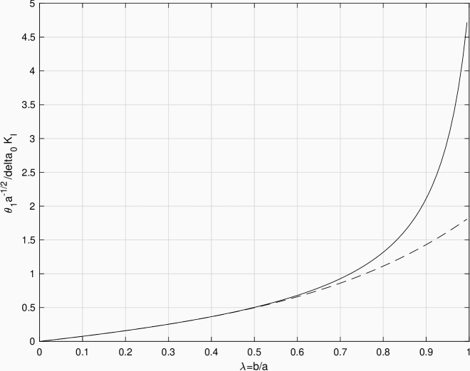
Figure 2: Normlized stress intensity factor $\theta_{1}a^{-1/2}K_{I}/\delta_{0}$ at the crack tip $r=a$ versus the parameter $\lambda$: the solid line corresponds to the exact formula (5.8), while the dashed line relates to the asymptotic formula (5.11).

Formulas (5.3) and (5.6) indicate that the normal stresses have the square root singularity as $r\to b^{-}$ and $r\to a^{+}$. This is consistent with the graphs of $\sigma_{z}(r,0)$ in the contact zone $0\leq r<b$ and for $r>a$ as $z=0$ (Fig.1). From the last formula we may immediately derive the stress intensity factor at the tip $r=a$ of the crack

$$K_{I}=\lim_{r\to a^{+}}\sqrt{2\pi(r-a)}\sigma_{z}(r,0).$$ (5.7)

It is given by

$$K_{I}=-2\sqrt{a}\sum_{m=0}^{\infty}A_{m}^{+}.$$ (5.8)

Note that the same formula is obtained directly from the expression (3.7) for the integral $\Phi_{2}^{+}(s)$ my employing the Abelian theorems for the Mellin transforms. In addition to the exact formula (5.8), it is possible to write a simple asymptotic formula in terms of $\lambda^{j}$. By virtue of the first formula in (3.10) and (5.8) we have

$$K_{I}=-2\sqrt{a}\lambda[a_{00}+\lambda a_{01}+\lambda^{2}(a_{02}+a_{10})+\lambda^{3}(a_{03}+a_{11})+\lambda^{4}(a_{04}+a_{12}+a_{20})+\ldots].$$ (5.9)

We next employ the recurrence relations (3.12) and deduce the expressions

$$a_{00}=-\frac{\delta^{*}}{\pi},\quad a_{10}=-\frac{\delta^{*}}{3\pi},\quad a_{20}=-\frac{\delta^{*}}{5\pi},$$

$$a_{01}=-\frac{4\delta^{*}}{\pi^{3}},\quad a_{02}=-\frac{16\delta^{*}}{\pi^{5}},\quad a_{11}=-\frac{4\delta^{*}}{3\pi^{3}},\quad a_{12}=-\frac{16\delta^{*}}{3\pi^{5}},$$

$$a_{03}=-\frac{4\delta^{*}}{\pi^{3}}\left(\frac{16}{\pi^{4}}+\frac{2}{9}\right),\quad a_{04}=-\frac{64\delta^{*}}{\pi^{5}}\left(\frac{4}{\pi^{4}}+\frac{1}{9}\right).$$ (5.10)

Here, as before, $\delta^{*}=2\delta(a\theta_{1}\sqrt{\pi})^{-1}$. Substituting these formulas into (5.9) yields the asymptotic expansion of the coefficient $K_{I}$ for small $\lambda$

$$K_{I}=\frac{4\sqrt{a}\delta_{0}}{\pi^{3/2}\theta_{1}}\left[\lambda+\frac{4\lambda^{2}}{\pi^{2}}+\left(\frac{16}{\pi^{4}}+\frac{1}{3}\right)\lambda^{3}\right.$$

$$\left.+\frac{4}{\pi^{2}}\left(\frac{16}{\pi^{4}}+\frac{5}{9}\right)\lambda^{4}+\left(\frac{256}{\pi^{8}}+\frac{112}{9\pi^{4}}+\frac{1}{5}\right)\lambda^{5}+O(\lambda^{6})\right],$$ (5.11)

where $\delta_{0}=\delta/a$. Referring to Fig. 2 we conclude that for $0<\lambda<0.6$ the asymptotic expansion (5.11) is in good agreement with the exact formula (5.8).

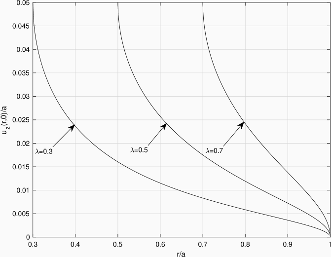
Figure 3: Normal displacement $u_{z}(r,0)/a$ for $b<r<a$ when $\lambda=0.3$, $\lambda=0.5$, and $\lambda=0.7$ for $\delta/a=0.05$.

The profile of the crack annular surface is described by the function $u_{z}(r,0^{+})=-a\theta_{1}\chi_{1}(r)$, $b\leq r\leq a$. Its integral representation is derived by the Mellin inversion of the function $\Phi_{1}^{-}(s)$ given by (3.7) that is

$$\chi_{1}(r)=\frac{1}{2\pi i}\int_{\cal L}\frac{\Psi^{+}(s)}{L^{-}(s)}\left(\frac{r}{a}\right)^{-s}ds$$

$$+\frac{1}{4\pi i}\int_{\cal L}\left\{L^{+}(s)\left[\Omega^{-}(s)-\frac{\delta^{*}}{s}\right]+\frac{\sqrt{\pi}\delta^{*}}{s}\right\}\left(\frac{r}{b}\right)^{-s}ds,\quad b<r<a.$$ (5.12)

As before we employ the theory of residues and, in addition, formula 9.121(26) from [11]

$$F\left(\frac{1}{2},\frac{1}{2};\frac{3}{2};x^{2}\right)=\frac{\sin^{-1}x}{x}.$$ (5.13)

This gives rise to the series representation for $b<r<a$

$$\chi_{1}(r)=-\frac{2\delta}{\pi a\theta_{1}}\sin^{-1}\frac{b}{r}+\frac{b}{\sqrt{\pi}r}\sum_{m=0}^{\infty}\frac{B^{-}_{m}}{2m+1}f_{m}\left(\frac{b^{2}}{r^{2}}\right)-\frac{2}{\sqrt{\pi}}\sum_{m=0}^{\infty}\frac{A^{+}_{m}}{2m+1}f_{m}\left(\frac{r^{2}}{a^{2}}\right),$$ (5.14)

where

$$f_{m}(x)=F\left(\frac{1}{2},m+\frac{1}{2};m+\frac{3}{2};x\right).$$ (5.15)

For according to formula 9.131(2) from [11] we can represent the function $f_{m}(x)$ for $x$ close to $1^{-}$ as

$$f_{m}(x)=\frac{\sqrt{\pi}(m+1/2)}{m!}\sum_{j=0}^{\infty}\left[\frac{\Gamma(m+j+1/2)}{j!}-\frac{\Gamma(m+j+1)\sqrt{1-x}}{\Gamma(j+3/2)}\right](1-x)^{j},$$ (5.16)

and, in the limit,

$$f_{m}(1^{-})=\frac{\pi(3/2)_{m}}{2m!}.$$ (5.17)

We wish now to verify that the normal displacement is continuous at the points $r=b$ and $r=a$. In view of (5.14) and (5.17) we deduce

$$\chi_{1}(b^{+})=-\frac{\delta}{a\theta_{1}}+\frac{1}{2}\sum_{m=0}^{\infty}\frac{B_{m}^{-}\Gamma(m+1/2)}{m!}-\frac{2}{\sqrt{\pi}}\sum_{m=0}^{\infty}\frac{A_{m}^{+}f_{m}(\lambda^{2})}{2m+1}$$ (5.18)

and

$$\chi_{1}(a^{-})=-\frac{2\delta}{\pi a\theta_{1}}\sin^{-1}\lambda+\frac{\lambda}{\sqrt{\pi}}\sum_{m=0}^{\infty}\frac{B_{m}^{-}f_{m}(\lambda^{2})}{2m+1}-\sum_{m=0}^{\infty}\frac{A_{m}^{+}\Gamma(m+1/2)}{m!}.$$ (5.19)

Analyze the expression (5.18) first. On employing formula (5.15), changing the order of summation in the second term in (5.18) we arrive at

$$\chi_{1}(b^{+})=-\frac{\delta}{a\theta_{1}}+\frac{1}{2}\sum_{m=0}^{\infty}\frac{\Gamma(m+1/2)}{m!}\left(B_{m}^{-}-\frac{2\lambda^{2m}}{\pi}\sum_{j=0}^{\infty}\frac{A_{j}^{+}}{m+j+1/2}\right).$$ (5.20)

Due to the first equation in (3.8) the expression in the brackets is equal to zero and therefore $u_{z}(b^{+})=-a\theta_{1}\chi_{1}(b^{+})=\delta$, and the normal displacement is continuous at $r=b$.

Similarly, formula (5.19) becomes

$$\chi_{1}(a^{-})=-\frac{2\delta\sin^{-1}\lambda}{\pi a\theta_{1}}-\sum_{m=0}^{\infty}\frac{\Gamma(m+1/2)}{m!}\left(A_{m}^{+}-\frac{\lambda^{2m+1}}{2\pi}\sum_{j=0}^{\infty}\frac{B_{j}^{-}}{m+j+1/2}\right).$$ (5.21)

Now it is turn of the second equation in the system (3.8). If, in addition, formulas (3.9) and (5.13) are used, then we have $\chi_{1}(a^{-})=0$, and the normal displacement is continuous at the point $r=a$ as well. The normalized displacements $u_{z}(r,0)/a$ for $\lambda=0.3$, $\lambda=0.5$, and $\lambda=0.7$ are plotted in Fig. 3.

6 Conclusion

We developed an analytical solution to two model problems of a penny-shaped crack when an annulus-shaped (model 1) or a disc-shaped (model 2) rigid inclusion planted between the crack faces. The method we proposed for these models recast the governing integral equations with the Weber–Sonin kernel on two segments as vector Riemann–Hilbert problems with a $3\times 3$ and $2\times 2$ triangular matrix coefficient. The solution presented for model 2 may be classified as an exact solution since it is given in terms of explicitly defined functions and exponentially convergent series whose coefficients are defined explicitly in terms of certain recurrence relations. Similar relations can be also written for model 1. For model 2, we derived representation formulas for the normal stress and displacement. For the stress intensity factor, in addition to the exact formula, we gave a simple asymptotic expansion in terms of $(b/a)^{n}$, $a$ and $b$ are the crack and inclusion radii, respectively, and $b<a$. For both models, we also found the canonical matrix of factorization and the partial indices of factorization which turn out to be zeros and therefore stable.

Data accessibility. No software generated data were created during this study.

Competing interests. We have no competing interests.

Funding statement. YAA thanks the Isaac Newton Institute for Mathematical Sciences, Cambridge, for support and hospitality during the programme Complex analysis: techniques, applications and computations, where a part of work on this paper was undertaken. This work was supported by EPSRC grant no EP/R014604/1 and the Simons Foundation.

References

• [1] Sneddon IN. 1946 The distribution of stress in the neighbourhood of a crack in an elastic solid. Proc. R. Soc. A 187, 229-260.
• [2] Mossakovskii VI. 1954 A fundamental mixed problem of the theory of elasticity for a half-space with a circular curve of separation of the boundary conditions. Prikl. Mat. Meh. 18 (1954), 187-196.
• [3] Mossakovskii VI, Rybka MT. 1964 Generalization of the Griffith-Sneddon criterion for the case of a nonhomogeneous body. J. Appl. Math. Mech. 28 (1964), 1277-1286.
• [4] Sneddon IN, Lowengrub M. 1969 Crack problems in the classical theory of elasticity. New York: John Wiley & Sons.
• [5] Willis JR. 1972 The penny-shaped crack on an interface. Quart. J. Mech. Appl. Math. 25(3). (1972), 367-385.
• [6] Antipov YA, Mkhitaryan SM. 2020 Correspondence principle in plane and axisymmetric mixed boundary-value problems of elasticity. Quart. Appl. Math. Published electronically on June 20 2019.
• [7] Selvadurai APS, Singh BM. 1984 On the expansion of a penny-shaped crack by a rigid circular disc inclusion. Int. J. Fracture 25, 69-77.
• [8] Antipov YA. 1987 Exact solution of the problem of pressing an annular stamp into a half-space. Dokl. Akad. Nauk Ukrain. SSR Ser. A 7, 29-33.
• [9] Antipov YA. 2015 Vector Riemann-Hilbert problem with almost periodic and meromorphic coefficients and applications. Proc. A. 471, no. 2180, 20150262,
• [10] Antipov YA, Mkhitaryan SM. 2017 A crack induced by a thin rigid inclusion partly debonded from the matrix, Quart. J. Mech. Appl. Math. 70, 153-185.
• [11] Gradshteĭn IS, Ryzhik IM. 2007 Table of Integrals, Series and Products. Oxford: Academic Press.
• [12] Antipov YA, Popov GYa, Yatsko SI. 1987 Solution of the problem of stress concentration around intersecting defects by using the Riemann problem with an infinite index. J. Appl. Math. Mech. 51, 357-365.
• [13] Antipov YA, Silvestrov VV. 2002 Factorization on a Riemann surface in scattering theory. Quart. J. Mech. Appl. Math. 55, 607-654.
• [14] Vekua NP.1967 Systems of Singular Integral Equations. Groningen: Noordhoff.
• [15] Gohberg IC, Krein MG. 1958 On the stability of a system of partial indices of the Hilbert problem for several unknown functions. Dokl. AN SSSR. 119, 854-857.