Motion of a Buoyant Vortex Patch

Banavara N. Shashikanth111Mechanical and Aerospace Engineering Department, MSC 3450, PO Box 30001, New Mexico State University, Las Cruces, NM 88003, USA. E-mail:shashi@nmsu.edu and Rangachari Kidambi 222Computational & Theoretical Fluid Dynamics Division, National Aerospace Laboratories, Bengaluru 560017, India. E-mail : kidambi@nal.res.in
Abstract

The motion of a two-dimensional buoyant vortex patch, i.e. a vortex patch with a uniform density different from the uniform density of the surrounding fluid, is analysed in terms of evolution equations for the motion of its centroid, deformation of its boundary and the strength of a vortex sheet which is essential to enforce pressure continuity across the boundary. The equations for the centroid are derived by a linear momentum analysis and that for the sheet strength by applying Eulerโ€™s equations on the boundary, while the boundary deformation is studied in the centroid-fixed frame. A complicated coupled set of equations is obtained which, to the best of our knowledge, has not been derived before. The evolution of the sheet strength is obtained as an integral equation. The equations are also examined in the limit of a patch of vanishing size or a buoyant point vortex.

1 Introduction

A vortex patch is a finite region of constant vorticity, surrounded by an irrotational flow. In the context of inviscid fluid flows, many studies have been published devoted to the dynamics of vortex patches in fluids of a single uniform density, henceforth also referred to as neutrally buoyant vortex patches. The Rankine and Kirchhoff vortex patches [20] are the simplest and best-known examples denoting a circular patch and an elliptical patch, respectively, rotating in fluid at rest at infinity. Deem and Zabusky in a pioneering paper [11] transformed the evolution equation of a patch to an evolution equation for its boundary alone. Based on this approach, named contour dynamics, they presented numerical evidence of a class of rotating isolated patches of more general shapes and a class of translating patch pairs of opposite-signed vorticity; see also [37]. The rotating solutions, termed as $V$-states, have $m$-fold symmetry ($m$ integer), i.e. $m$ axes of symmetry. The Kirchhoff patch corresponds to $m=2$. Burbea [7] used analytical techniques to derive some of the $V$-states. Moore and Saffman [24]โ€”and later Kida [18]โ€”studied, as a first level approximation, the effect of a uniform shear flow, i.e. a flow in which the velocity field is linear in the coordinates, on the dynamics of an isolated elliptic patch. The patch continues to retain its elliptic form but its aspect ratio and angular velocity get modified. A Hamiltonian generalization of this is the $N$ patch moment model of Melander, Zabusky and Styczek [23]. More investigations about the opposite-signed translating pair were made by Pierrehumbert [25] and Yang and Kubota [36]. Saffman and Szeto [31] investigated same-signed patch pairs that rotate about each other. Linear and rotating arrays of vortex patches have also been studied; see, for example, [32, 26, 9]. Dritschel [10] has used contour dynamics and its improvements like contour surgery to study different features of patch evolution such as filamentation and merging. Patches have also been investigated in a Hamiltonian framework. Marsden and Weinstein [22], among other things, placed the Hamiltonian structure of singular vortex models, such as point vortices and vortex filaments, as also that of a vortex patch, in the wider framework of modern theories of Hamiltonian systems with symmetry and reduction. Exploiting this Hamiltonian structure, the nonlinear stability of patches was analyzed in [33, 34, 35].

On the other hand, the motion of vortex patches, with density variations present, even though very relevant to geophysical and atmospheric flows, has attracted relatively less attention. Arendt [1, 2] studied such patches as a model of sunspots while [3] presented point vortex models of vortex motion in a stratified fluid. Steady stratification and an essentially hydrostatic pressure field were assumed. An important finding of Arendtโ€™s work is that such vortices, under the influence of the stratification, have a self-propulsion transverse to gravity and that this propulsion is logarithmically singular in the ratio of the cross-section to the density scale height. In an earlier paper, Saffman [29] developed a model for a buoyant point vortex pair in a stratified atmosphere and concluded that they performed oscillatory motions in a vertical direction, the distance between them remaining constant. Hill [16] numerically confirmed Saffmanโ€™s predictions for small times. High frequency oscillations were found to be possible in the motion of a single, buoyant rectilinear vortex, of small core cross-section and that neglecting the finite cross section except in the buoyancy term, leads to the point vortex equations under the action of a force [30]. Both Arendtโ€™s and Saffmanโ€™s papers also contain references to some earlier work on the topic.

Modeling vortex interactions in the presence of a continuously varying density field is, in general, a very difficult task; especially obtaining analogues of some well-studied low-dimensional models in homogeneous flows, such as an isolated vortex patch or the classical $N$-point-vortex model. A relatively simpler problem is where the density field is modeled as a step function. Specifically, the uniform density of the patch $\rho_{i}$ is assumed to be different from the uniform density $\rho_{o}$ of the fluid external to it. A popular assumption in the literature on surface-tension-free interfaces has been the use of pressure continuity at the interface. For patches with density jumps, Eulerโ€™s equations implies a jump in the tangential velocity at the boundary and consequently a vortex sheet. The resulting models, involving vortex patches bounded by vortex sheets, have been referred to in the literature as Prandtl-Batchelor flows or sheet patches [30]; we use the term bouyant vortex patch (BVP) in this paper. Note that, in these models, vorticity generation happens only at the patch boundary, due to baroclinicity; elsewhere, the fluid is barotropic. Sheet patch studies have mostly involved computation of equilibria in a variety of background flows ([12], [17], [38]). For example, in the important paper of Kao & Caflisch [17] invariant translating vortex patch shapes as a function of density ratio and circulation were computed. For a given density ratio below a limiting value, a unique shape, translating with constant velocity, was found. In such equilibria studies, the vortex sheet strength at the patch boundary is assumed constant. Evolution equations for varying sheet strength have been typically obtained in models of irrotational flows, for example, the paper by Baker and Moore [4] that computes the evolution of a buoyant air bubble, by generalising the Birkhoff-Rott equation for vortex sheet evolution in a single density fluid, and the paper by Baker, Meiron and Orszag [5] that computes free-surface flows by modelling the free surfaces as vortex sheets; a Fredholm integral equation governing the sheet strength is derived. The jump in the tangential velocity for a buoyant patch may be contrasted with the continuity of the velocity at the boundary of a neutrally buoyant vortex patch. However, it appears possible to consider a situation of continuous velocity, with attendant pressure discontinuity, at the interface; this possibly is sketched in Appendix C.

More recently, Ravichandran et al [28] presented, apart from a DNS study, a simple model for the evolution of the centroid of a buoyant circular patch, to demonstrate the โ€˜lift-inducedโ€™ collapse of a vortex dipole. The evolution equation for the patch centroid (Eq.(3) of that paper) is written in an ad hoc manner. Carpenter & Guha [8] also present an ad hoc model for buoyant point vortices. The present analysis will clarify issues relevant to these models.

The main goal of the present work is to derive the correct equations governing an isolated buoyant vortex patch. First, applying the momentum theorem to a standard control volume, that includes the patch and surrounding fluid, the equation governing the motion of the centroid of the patch is derived. Along with the linear momentum equation, the equation governing the evolution of the buoyant patch boundary which will, in general, deform, is analyzed. Exploiting the inherent $\operatorname{SE}(2)$ symmetry in the flow, use is made of a centroid-fixed translating frame in deriving the equations of the boundary which allows for a decomposition of the deformation and translation velocity fields. Finally, baroclinicity at the patch boundary creates a vortex sheet of time-varying strength. It is shown in detail how a single integral equation for the evolution of the sheet strength can be obtained and how the combined set of equations can then, in principle, be propagated in time. To the best of our knowledge, a set of such general coupled equations governing the deformation and translation of a buoyant vortex patch of any smooth shape has not been derived before. This paper only touches upon numerically solving these equations, a more detailed exploration alone these lines is planned for the future. But by deriving these equations, we want to exhibit the enormous complexities that enter the mathematical model of a classical vortex patch by simply relaxing the assumption of homogeneous density. Last, but not least, the point vortex limit is examined.

Note that an alternative to using a vortex sheet is to model the irrotational flows generated by the sheet using Zakharovโ€™s formulation for the motion of free surfaces in the Hamiltonian variables of the boundary position and the velocity potential function on the boundary. Such an approach is used in the problems considered in, for example, the papers [6, 21]. But evolving the system involves extensive integration of Neumann or Dirichlet problems. Moreover, the boundary is not โ€˜freeโ€™, and so the Zakharov formulations would entail the additional task of dealing with the pressure on the boundary. As is well-known, advantages afforded by a vortex sheet is that it avoids the explicit use of pressure and the need for integrating Laplaceโ€™s equation in the domain.

The paper is organized as follows. In Section 2, we present the linear momentum analysis for a buoyant vortex patch and derive the equation governing the motion of the vortex centroid. In Section 3, we present the decomposition of the velocity fields and the evolution equations for the patch boundary, in both the spatially-fixed and centroid-fixed frames. In Section 4, we present the pressure continuity condition and the vortex sheet strength equation that follows. This is followed by a brief outline of an algorithmic procedure for solving all the governing equations. Finally, a brief examination of the equations in several limits, including the point vortex limit, is presented. In Section 5, some concluding remarks are made.

To keep the paper uncluttered, most of the derivations are relegated to the Appendices. Moreover, to avoid a large number of overhead arrows or boldface symbols throughout the paper, we have chosen to represent vectors (except for unit vectors) and scalars in the same manner without any distinguishing notation.

2 Linear momentum analysis

Consider a buoyant vortex patch with uniform vorticity (function) $\omega$ in a time varying domain $D_{v}(t)\subset\mathbb{R}^{2}$, with boundary $\partial D_{v}(t)$ and invariant area $A$. The fluid in the domain $D(t):=\mathbb{R}^{2}\backslash D_{v}(t)$ is assumed irrotational. Moreover, the fluid is incompressible everywhere but with different densities (per unit area) inside and outside the patch, $\rho_{i}$ and $\rho_{o}$. The fluid is in an uniform gravitational field pointing in the $-\hat{j}$ direction.

Refer to caption
Figure 1: Schematic for the buoyant vortex patch. Gravity points down.

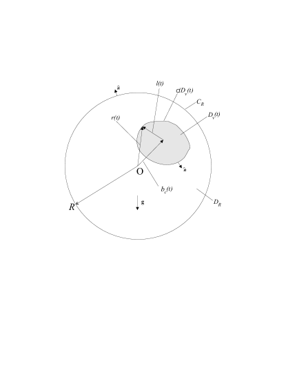
Now consider a fixed control volume in the shape of a disc $D_{R}$ of radius $R$, centered at point $O$, with boundary $C_{R}$. Let $\tilde{D}(t):=D(t)\cap D_{R}$. Take $O$ to be the origin of a spatially-fixed frame and let $r$ denote the position vector in this frame. In addition, let $b_{c}(t)$ denote the position vector of the centroid of the patch in this frame, and write $r=b_{c}+l$. By definition of the centroid, at any time $t$,

$$\int_{D_{v}(t)}l\;dA=0$$

Let $\hat{n}_{v}$ be the unit outward normal on the patch (i.e. pointing away from the patch) and $n$ the unit normal on $C_{R}$. A schematic of the situation is shown in figure 1.

The problem of the BVP is formulated as follows. The fluid flow in $D_{v}$ is governed by a streamfunction obeying

$$\nabla^{2}\psi_{i}(r,t)=-\omega,$$

and the corresponding velocity field $v_{i}=J\nabla\psi_{i}$, where $r$ is the position vector in a spatially-fixed frame and $J:=\left(\begin{array}[]{cc}0&1\\ -1&0\end{array}\right)$.

The fluid flow in $D$ is governed by a velocity potential function $\phi_{o}$ satisfying the following Neumann problem:

$\displaystyle\nabla^{2}\phi_{o}$ $\displaystyle=0\>{\rm in}\>D,$
$\displaystyle\nabla\phi_{o}\cdot\hat{n}$ $\displaystyle=v_{i}\cdot\hat{n}\>{\rm on}\>\partial D_{v},\quad\phi_{o}\rightarrow{\rm constant}\>{\rm as}\>r\rightarrow\infty,$

and the corresponding velocity field is given by $v_{0}=\nabla\phi_{o}$.

Applying the momentum theorem to the fluid in $D_{R}$ (details in Appendix A), we have

Vcร—ฯoโ€‹ฮ“oโ€‹k^+ฯoโ€‹ddโ€‹tโ€‹โˆฎโˆ‚Dvโ€‹(t)lร—(n^ร—vo)โ€‹๐‘‘ssubscript๐‘‰๐‘subscript๐œŒ๐‘œsubscriptฮ“๐‘œ^๐‘˜subscript๐œŒ๐‘œ๐‘‘๐‘‘๐‘กsubscriptcontour-integralsubscript๐ท๐‘ฃ๐‘ก๐‘™^๐‘›subscript๐‘ฃ๐‘œdifferential-d๐‘ \displaystyle V_{c}\times\rho_{o}\Gamma_{o}\hat{k}+\rho_{o}\frac{d}{dt}\oint_{\partial D_{v}(t)}l\times\left(\hat{n}\times v_{o}\right)\;ds
โˆ’ฯiโ€‹ddโ€‹tโ€‹โˆฎโˆ‚Dvโ€‹(t)lร—(n^ร—vi)โ€‹๐‘‘s=(ฯoโˆ’ฯi)โ€‹Aโ€‹gโ€‹j^subscript๐œŒ๐‘–๐‘‘๐‘‘๐‘กsubscriptcontour-integralsubscript๐ท๐‘ฃ๐‘ก๐‘™^๐‘›subscript๐‘ฃ๐‘–differential-d๐‘ subscript๐œŒ๐‘œsubscript๐œŒ๐‘–๐ด๐‘”^๐‘—\displaystyle\hskip 72.26999pt-\rho_{i}\frac{d}{dt}\oint_{\partial D_{v}(t)}l\times\left(\hat{n}\times v_{i}\right)\;ds=(\rho_{o}-\rho_{i})Ag\hat{j} (1)

where $V_{c}$ is the velocity of the centroid and

ฮ“o:=โˆฎโˆ‚Dvโ€‹(t)voโ‹…t^โ€‹๐‘‘sassignsubscriptฮ“๐‘œsubscriptcontour-integralsubscript๐ท๐‘ฃ๐‘กโ‹…subscript๐‘ฃ๐‘œ^๐‘กdifferential-d๐‘ \Gamma_{o}:=\oint_{\partial D_{v}(t)}v_{o}\cdot\hat{t}ds

is the circulation of the outer flow. Since the outer flow is irrotational, Stokesโ€™ theorem implies that $\Gamma_{o}$ is the same for any closed circuit in the outer fluid that encloses the vortex patch. On the other hand,

ฮ“i:=โˆฎโˆ‚Dvโ€‹(t)viโ‹…t^โ€‹๐‘‘s=ฯ‰โ€‹A,assignsubscriptฮ“๐‘–subscriptcontour-integralsubscript๐ท๐‘ฃ๐‘กโ‹…subscript๐‘ฃ๐‘–^๐‘กdifferential-d๐‘ ๐œ”๐ด\Gamma_{i}:=\oint_{\partial D_{v}(t)}v_{i}\cdot\hat{t}ds=\omega A,

(the last equation again following from Stokesโ€™ theorem) is the circulation of the inner flow and is fixed by the patch parameters $\omega$ and $A$. By Kelvinโ€™s circulation theorem, both $\Gamma_{o}$ and $\Gamma_{i}$ are invariant in time. This is easily seen since $d\Gamma/dt=-\oint_{\beta}dp/\rho=0$ for any closed circuit $\beta$ lying either in the outer fluid or in the inner fluid.

A straightforward rearrangement gives the following equation

$\displaystyle\Gamma_{o}$ =ฯ‰โ€‹A+โˆฎโˆ‚Dvโ€‹(t)ฮณโ€‹๐‘‘sabsent๐œ”๐ดsubscriptcontour-integralsubscript๐ท๐‘ฃ๐‘ก๐›พdifferential-d๐‘ \displaystyle=\omega A+\oint_{\partial D_{v}(t)}\gamma ds (2)

where

ฮณโ€‹(s,t):=(voโˆ’vi)โ‹…t^assign๐›พ๐‘ ๐‘กโ‹…subscript๐‘ฃ๐‘œsubscript๐‘ฃ๐‘–^๐‘ก\gamma(s,t):=(v_{o}-v_{i})\cdot\hat{t}

is the total slip velocity field on the patch boundary. This slip field consists of two contributionsโ€“the slip due to the vortex sheet whose strength is one of the variables of the system and another slip field generated by the instantaneous translation motion. Both these are described later. It follows that โˆฎโˆ‚Dvโ€‹(t)ฮณโ€‹๐‘‘ssubscriptcontour-integralsubscript๐ท๐‘ฃ๐‘ก๐›พdifferential-d๐‘ \oint_{\partial D_{v}(t)}\gamma\,ds is also invariant in time, though ฮณโ€‹(s,t)๐›พ๐‘ ๐‘ก\gamma(s,t) is in general not. In other words, as in the work of [5], there is no global baroclinic generation of vorticity, but the variation in ฮณโ€‹(s,t)๐›พ๐‘ ๐‘ก\gamma(s,t) may be identified with local baroclinic generation of vorticity.

In equationย (2), the $dV_{c}/dt$ term does not appear explicitly. The role of this term is seen more clearly in the next section, where the equation is written in a different way.

3 Deformations of buoyant vortex patches

The natural next question to ask is how the centroid motion and the boundary deformation are linked to each other, and this is examined in this section.

The boundary deformation is caused by the vorticity in the patch and the essential vortex sheet which enforces the pressure continuity condition. The buoyant force on the patch causes the centroid to move and the patch to instantaneously translate which generates irrotational flows both inside and outside the patch. These flows will be modeled as Kirchhoff flows associated with the instantaneous rigid boundary shape, and are discussed more below.

We first write the equations in a spatially-fixed frame. The boundary of the patch is viewed as the image of smooth maps, $\partial D_{v}:S^{1}\rightarrow\mathbb{R}^{2}$. Denote by Cโ€‹(s,t)๐ถ๐‘ ๐‘กC(s,t) the coordinates of the image which is a smooth curve in $\mathbb{R}^{2}$, and by Cยฏโ€‹(s,t)ยฏ๐ถ๐‘ ๐‘ก\bar{C}(s,t) the same curve with respect to the translating frame defined in the next section. Assuming the patch motion at every instant to be decomposable into a rigid translation and a deformation, the fluid flow in the inner region $D_{v}$ is governed by the following streamfunction and velocity field

$$\displaystyle\psi_{i}(r,t)=\psi_{Di}(r,t)+\psi_{Ti}(r,t),\,\,v_{i}(r,t)=v_{Di}(r,t)+V_{c}(t),$$ (3)

where the subscripts $D,T$ and $i$ stand for deformation, translation and inner. The deformation field $\psi_{Di}$ is the sum of two components, $\psi_{p}$ and ฯˆsโ€‹isubscript๐œ“๐‘ ๐‘–\psi_{si}, which indicate respectively the contributions of the patch and the bounding vortex sheet. Thus the various component streamfunctions are

$\displaystyle\psi_{p}(r,t)$ $\displaystyle=\frac{\omega}{2\pi}\int_{D_{v}(t)}\log\mid r-\tilde{r}\mid\;d\tilde{A},$
ฯˆsโ€‹iโ€‹(r,t)subscript๐œ“๐‘ ๐‘–๐‘Ÿ๐‘ก\displaystyle\psi_{si}(r,t) =12โ€‹ฯ€โ€‹โˆฎCฮณsโ€‹(s~,t)โ€‹logโกโˆฃrโˆ’r~โˆฃโ€‹dโ€‹s~,r~:=rโ€‹(s~)formulae-sequenceabsent12๐œ‹subscriptcontour-integral๐ถsubscript๐›พ๐‘ ~๐‘ ๐‘กdelimited-โˆฃโˆฃ๐‘Ÿ~๐‘Ÿ๐‘‘~๐‘ assign~๐‘Ÿ๐‘Ÿ~๐‘ \displaystyle=\frac{1}{2\pi}\oint_{C}\gamma_{s}(\tilde{s},t)\log\mid r-\tilde{r}\mid\;d\tilde{s},\quad\tilde{r}:=r(\tilde{s})
$\displaystyle\psi_{T}(r,t)$ $\displaystyle=(V_{c}(t)\times r)\cdot\hat{k}$

where ฮณ๐”ฐโ€‹(s,t)subscript๐›พ๐”ฐ๐‘ ๐‘ก\gamma_{\mathfrak{s}}(s,t) is the strength distribution of the vortex sheet, s๐‘ s is the boundary curve parameter and $V_{c}(t)$ is the velocity of the patch centroid. $\psi_{Ti}$ is the harmonic streamfunction of the internal Kirchhoff flow generated by the instantaneous rigid body translation of the patch. It may be recalled that the velocity field of this flow is equal to $V_{c}(t)$ everywhere in the patch [20]. The other component velocity fields are

$\displaystyle v_{p}(r,t)$ $\displaystyle=-\frac{1}{2\pi}\omega\hat{k}\times\int_{D_{v}(t)}\nabla_{r}\log\mid r-\tilde{r}\mid\;d\tilde{A},$ (4)
vsโ€‹iโ€‹(r,t)subscript๐‘ฃ๐‘ ๐‘–๐‘Ÿ๐‘ก\displaystyle v_{si}(r,t) =โˆ’12โ€‹ฯ€โ€‹โˆฎCฮณ๐”ฐโ€‹(s~,t)โ€‹k^ร—rโˆ’r~โˆฃrโˆ’r~โˆฃ2โ€‹๐‘‘s~,rโ€‹(s)โˆˆDv,formulae-sequenceabsent12๐œ‹subscriptcontour-integral๐ถsubscript๐›พ๐”ฐ~๐‘ ๐‘ก^๐‘˜๐‘Ÿ~๐‘Ÿsuperscriptdelimited-โˆฃโˆฃ๐‘Ÿ~๐‘Ÿ2differential-d~๐‘ ๐‘Ÿ๐‘ subscript๐ท๐‘ฃ\displaystyle=-\frac{1}{2\pi}\oint_{C}\gamma_{\mathfrak{s}}(\tilde{s},t)\hat{k}\times\frac{r-\tilde{r}}{\mid r-\tilde{r}\mid^{2}}\;d\tilde{s},\quad r(s)\in D_{v}, (5)

The fluid flow in $D$ is governed by the following streamfunction and velocity field

$\displaystyle\psi_{o}(r,t)$ $\displaystyle=\psi_{Do}(r,t)+\psi_{To}(r,t),\quad v_{o}(r,t)=v_{Do}(r,t)+v_{To}(r,t),$ (6)

where again the deformation field $\psi_{Do}$ is the sum of two components $\psi_{p}$ and ฯˆsโ€‹osubscript๐œ“๐‘ ๐‘œ\psi_{so}. Note that the velocity induced by a vortex patch is continuous across the boundary so that $v_{p}$ for points in $D$ is given by the same expression asย (4). The vortex sheet velocity field expression is also the same as ย (5) but recall [30] that the expression leads to a jump in the tangential velocity across the boundary. The Kirchhoff flows also induce a discontinuous tangential velocity at the boundary. $\psi_{To}$ is the harmonic conjugate of $\phi_{To}$ which satisfies the following Neumann problem,

$\displaystyle\nabla^{2}\phi_{To}$ $\displaystyle=0\>{\rm in}\>D,$
$\displaystyle\nabla\phi_{To}\cdot\hat{n}(\equiv v_{To}\cdot\hat{n})$ $\displaystyle=V_{c}\cdot\hat{n}\>{\rm on}\>\partial D_{v},\quad\phi_{To}\rightarrow{\rm constant}\>{\rm as}\>r\rightarrow\infty$

The above problem, when written in a body-fixed frame, is recognized as the external Kirchhoff flow generated by the instantaneous rigid body translation. Recall that this is the external irrotational incompressible flow induced by a moving rigid body. Kirchhoff [19, 20] showed that in general the velocity potential function of such a flow, referred to a body-fixed frame,333Though the body-fixed frame used by Kirchhoff is a classical concept, the problem is sometimes confused with the flow described in a non-inertial frame. In the former, each vector is expressed in terms of the instantaneous body-fixed frame and, except for the position vector, differs from the vector expressed in the spatially-fixed frame by the action of the instantaneous rotation matrix. For a purely translating frame, as in our problem, the vectors in the two frames are identical; see, for example, Goldstein [14] for a discussion of such frames. can be expressed in terms of the bodyโ€™s instantaneous velocities and unit potential functions that depend solely on the bodyโ€™s rigid shape. In the current problem, since the bodyโ€™s shape is not rigid the unit potential functions are time-dependent and, at each instant, are the unit potentials corresponding to the instantaneous shape.

Let $\tilde{\phi}_{To}(l,t):=\phi_{To}(r,t)$, then

$\displaystyle\tilde{\phi}_{To}(l,t)$ $\displaystyle=V_{cx}(t)a(l,\bar{C})+V_{cy}(t)b(l,\bar{C}),$
$\displaystyle\Rightarrow v_{To}(l,t):=\nabla\tilde{\phi}_{To}(l,t)$ $\displaystyle=E(l,\bar{C})\cdot V_{c}(t)$

where $E$ is a $2\times 2$ matrix of the first order spatial derivatives of the unit potentials $a$ and $b$. The unit potentials typically have analytic expressions only for simple shapes, or shapes obtained from conformal maps. For arbitrary shapes, a Laplace equation solver may have to be appended that numerically computes these functions at each instant in a neighborhood of $\bar{C}$. Recall that the sheet strength distribution is given by

ฮณsโ€‹(s,t)=(vsโ€‹oโˆ’vsโ€‹i)โ‹…t^subscript๐›พ๐‘ ๐‘ ๐‘กโ‹…subscript๐‘ฃ๐‘ ๐‘œsubscript๐‘ฃ๐‘ ๐‘–^๐‘ก\gamma_{s}(s,t)=(v_{so}-v_{si})\cdot\hat{t}

with vsโ€‹o,vsโ€‹isubscript๐‘ฃ๐‘ ๐‘œsubscript๐‘ฃ๐‘ ๐‘–v_{so},v_{si} evaluated for boundary points and given by standard vortex sheet relations [30]

vsโ€‹o=ฮณs2โ€‹t^+Cโ€‹Pโ€‹V,vsโ€‹i=โˆ’ฮณs2โ€‹t^+Cโ€‹Pโ€‹Vformulae-sequencesubscript๐‘ฃ๐‘ ๐‘œsubscript๐›พ๐‘ 2^๐‘ก๐ถ๐‘ƒ๐‘‰subscript๐‘ฃ๐‘ ๐‘–subscript๐›พ๐‘ 2^๐‘ก๐ถ๐‘ƒ๐‘‰\displaystyle v_{so}=\frac{\gamma_{s}}{2}\hat{t}+CPV,\,v_{si}=-\frac{\gamma_{s}}{2}\hat{t}+CPV (7)

where $CPV$ denotes the Cauchy Principal Value of the contour integral in ย (5) when evaluated for points on the boundary. Keeping in mind that for the vortex sheet vsโ€‹oโ€‹(r,t)โ‹…n^=vsโ€‹iโ€‹(r,t)โ‹…n^โ‹…subscript๐‘ฃ๐‘ ๐‘œ๐‘Ÿ๐‘ก^๐‘›โ‹…subscript๐‘ฃ๐‘ ๐‘–๐‘Ÿ๐‘ก^๐‘›v_{so}(r,t)\cdot\hat{n}=v_{si}(r,t)\cdot\hat{n} on $\partial D_{v}$, one obtains the required continuity of normal velocity at the boundary, $v_{o}(r,t)\cdot\hat{n}=v_{i}(r,t)\cdot\hat{n}$ on $\partial D_{v}$.

Moreover, $\gamma$ and ฮณssubscript๐›พ๐‘ \gamma_{s} are related by

$\displaystyle\gamma$ $\displaystyle=\gamma_{\mathfrak{s}}+[(E-I)\cdot V_{c}]\cdot\hat{t}$

from which it follows that

โˆฎCยฏฮณโ€‹๐‘‘s=โˆฎCยฏฮณ๐”ฐโ€‹๐‘‘s,subscriptcontour-integralยฏ๐ถ๐›พdifferential-d๐‘ subscriptcontour-integralยฏ๐ถsubscript๐›พ๐”ฐdifferential-d๐‘ \oint_{\bar{C}}\gamma\;ds=\oint_{\bar{C}}\gamma_{\mathfrak{s}}\;ds,

since the Kirchhoff flows have zero circulations associated with them. Referring to equationย (2), this implies that $\Gamma_{o}$ is the sum of the circulations due to the vortex patch and the vortex sheet.

The evolution of the patch boundary is given, as usual, by

$\displaystyle\frac{\partial C}{\partial t}$ $\displaystyle=(v_{i}\cdot\hat{n})\hat{n}=\left(J\nabla\psi_{i}\cdot\hat{n}\right)\hat{n},$ (8)

where $J:=\left(\begin{array}[]{cc}0&1\\ -1&0\end{array}\right)$. Note that only the normal component of the velocity field contributes to the evolution of Cโ€‹(s,t)๐ถ๐‘ ๐‘กC(s,t).

3.1 Centroid-fixed translating frame

With a view to obtaining an equation for the centroid velocity $V_{c},$ we now write ย (2) and ย (3) in a centroid-fixed frame translating parallel to the stationary frame with origin at the patch centroid. With respect to this frame, ย (3) can be written as

$\displaystyle\psi_{i}(r,t)$ $\displaystyle=\tilde{\psi}_{i}(l,t)$
=ฯ‰2โ€‹ฯ€โ€‹โˆซDvโ€‹(t)logโกโˆฃlโˆ’l~โˆฃโ€‹dโ€‹A~+12โ€‹ฯ€โ€‹โˆฎCยฏฮณ๐”ฐโ€‹(s~,t)โ€‹logโกโˆฃlโˆ’l~โˆฃโ€‹dโ€‹s~+(Vcร—l)โ‹…k^โŸฯˆiโ€‹(l,t)absentsubscriptโŸ๐œ”2๐œ‹subscriptsubscript๐ท๐‘ฃ๐‘กdelimited-โˆฃโˆฃ๐‘™~๐‘™๐‘‘~๐ด12๐œ‹subscriptcontour-integralยฏ๐ถsubscript๐›พ๐”ฐ~๐‘ ๐‘กdelimited-โˆฃโˆฃ๐‘™~๐‘™๐‘‘~๐‘ โ‹…subscript๐‘‰๐‘๐‘™^๐‘˜subscript๐œ“๐‘–๐‘™๐‘ก\displaystyle=\underbrace{\frac{\omega}{2\pi}\int_{D_{v}(t)}\log\mid l-\tilde{l}\mid\;d\tilde{A}+\frac{1}{2\pi}\oint_{\bar{C}}\gamma_{\mathfrak{s}}(\tilde{s},t)\log\mid l-\tilde{l}\mid\;d\tilde{s}+(V_{c}\times l)\cdot\hat{k}}_{\psi_{i}(l,t)}
$\displaystyle\hskip 144.54pt+(V_{c}\times b)\cdot\hat{k},$ (9)

$l$ being the position vector in this frame. It is important to note that for points on the boundary $l$ is exactly the same as Cยฏโ€‹(s,t)ยฏ๐ถ๐‘ ๐‘ก\bar{C}(s,t) the boundary curve coordinates in this frame. The last term on the right is a purely time-dependent function. The curve evolution equation in the translating frame is seen to be (details in Appendix B)

$\displaystyle\frac{\partial\bar{C}}{\partial t}$ ={(โˆ’ฯ‰2โ€‹ฯ€โ€‹โˆฎCยฏlogโกโˆฃlโˆ’l~โˆฃโ€‹t^~โ€‹dโ€‹s~โˆ’12โ€‹ฯ€โ€‹โˆฎCฮณ๐”ฐโ€‹(s~,t)โ€‹k^ร—lโˆ’l~โˆฃlโˆ’l~โˆฃ2โ€‹๐‘‘s~)โ‹…n^}โ€‹n^absentโ‹…๐œ”2๐œ‹subscriptcontour-integralยฏ๐ถdelimited-โˆฃโˆฃ๐‘™~๐‘™~^๐‘ก๐‘‘~๐‘ 12๐œ‹subscriptcontour-integral๐ถsubscript๐›พ๐”ฐ~๐‘ ๐‘ก^๐‘˜๐‘™~๐‘™superscriptdelimited-โˆฃโˆฃ๐‘™~๐‘™2differential-d~๐‘ ^๐‘›^๐‘›\displaystyle=\bigg{\{}\left(-\frac{\omega}{2\pi}\oint_{\bar{C}}\log\mid l-\tilde{l}\mid\tilde{\hat{t}}\;d\tilde{s}-\frac{1}{2\pi}\oint_{C}\gamma_{\mathfrak{s}}(\tilde{s},t)\hat{k}\times\frac{l-\tilde{l}}{\mid l-\tilde{l}\mid^{2}}\;d\tilde{s}\right)\cdot\hat{n}\bigg{\}}\hat{n} (10)

Due to the $\operatorname{SE}(2)$ symmetries in the streamfunctions of the patch and the sheet the deformation equation in the centroid-fixed frame becomes independent of the drift of the centroid. To predict the latter one needs the linear momentum equationย (1). The $\operatorname{SE}(2)$ symmetries mean that the velocity fields due to these streamfunctions are the same relative to the patch regardless of its absolute location and orientation in the plane.

Noting that equationย (1) is equally valid in the centroid-fixed frame, rewrite it as:

Vcร—ฯoโ€‹ฮ“oโ€‹k^+ฯoโ€‹ddโ€‹tโ€‹โˆฎCยฏlร—(n^ร—(voโˆ’vi))โ€‹๐‘‘ssubscript๐‘‰๐‘subscript๐œŒ๐‘œsubscriptฮ“๐‘œ^๐‘˜subscript๐œŒ๐‘œ๐‘‘๐‘‘๐‘กsubscriptcontour-integralยฏ๐ถ๐‘™^๐‘›subscript๐‘ฃ๐‘œsubscript๐‘ฃ๐‘–differential-d๐‘ \displaystyle V_{c}\times\rho_{o}\Gamma_{o}\hat{k}+\rho_{o}\frac{d}{dt}\oint_{\bar{C}}l\times\left(\hat{n}\times(v_{o}-v_{i})\right)\;ds
+(ฯoโˆ’ฯi)โ€‹ddโ€‹tโ€‹โˆฎCยฏlร—(n^ร—vi)โ€‹๐‘‘s=(ฯoโˆ’ฯi)โ€‹Aโ€‹gโ€‹j^subscript๐œŒ๐‘œsubscript๐œŒ๐‘–๐‘‘๐‘‘๐‘กsubscriptcontour-integralยฏ๐ถ๐‘™^๐‘›subscript๐‘ฃ๐‘–differential-d๐‘ subscript๐œŒ๐‘œsubscript๐œŒ๐‘–๐ด๐‘”^๐‘—\displaystyle\hskip 72.26999pt+(\rho_{o}-\rho_{i})\frac{d}{dt}\oint_{\bar{C}}l\times\left(\hat{n}\times v_{i}\right)\;ds=(\rho_{o}-\rho_{i})Ag\hat{j}

Now apply the vector identityย (A1), and another, to write

โˆฎCยฏlร—(n^ร—vi)โ€‹๐‘‘ssubscriptcontour-integralยฏ๐ถ๐‘™^๐‘›subscript๐‘ฃ๐‘–differential-d๐‘ \displaystyle\oint_{\bar{C}}l\times\left(\hat{n}\times v_{i}\right)\;ds $\displaystyle=\int_{D_{v}}l\times\omega\;dA-\int_{D_{v}}v_{i}\;dA,$
$\displaystyle=\int_{D_{v}}l\times\omega\;dA-\hat{k}\times\int_{D_{v}}\nabla_{l}\Psi_{i}\;dA-\int_{D_{v}}V_{c}\;dA,$
=โˆซDvlร—ฯ‰โ€‹๐‘‘Aโˆ’k^ร—โˆฎCยฏฮจiโ€‹n^โ€‹๐‘‘sโˆ’Vcโ€‹A,absentsubscriptsubscript๐ท๐‘ฃ๐‘™๐œ”differential-d๐ด^๐‘˜subscriptcontour-integralยฏ๐ถsubscriptฮจ๐‘–^๐‘›differential-d๐‘ subscript๐‘‰๐‘๐ด\displaystyle=\int_{D_{v}}l\times\omega\;dA-\hat{k}\times\oint_{\bar{C}}\Psi_{i}\hat{n}\;ds-V_{c}A,
=โˆซDvlร—ฯ‰โ€‹๐‘‘Aโˆ’โˆฎCยฏฮจiโ€‹t^โ€‹๐‘‘sโˆ’Vcโ€‹Aabsentsubscriptsubscript๐ท๐‘ฃ๐‘™๐œ”differential-d๐ดsubscriptcontour-integralยฏ๐ถsubscriptฮจ๐‘–^๐‘กdifferential-d๐‘ subscript๐‘‰๐‘๐ด\displaystyle=\int_{D_{v}}l\times\omega\;dA-\oint_{\bar{C}}\Psi_{i}\hat{t}\;ds-V_{c}A

so that

ddโ€‹tโ€‹โˆฎCยฏlร—(n^ร—vi)โ€‹๐‘‘s=โˆ’ddโ€‹tโ€‹โˆฎCยฏฮจiโ€‹t^โ€‹๐‘‘sโˆ’Aโ€‹dโ€‹Vcdโ€‹t๐‘‘๐‘‘๐‘กsubscriptcontour-integralยฏ๐ถ๐‘™^๐‘›subscript๐‘ฃ๐‘–differential-d๐‘ ๐‘‘๐‘‘๐‘กsubscriptcontour-integralยฏ๐ถsubscriptฮจ๐‘–^๐‘กdifferential-d๐‘ ๐ด๐‘‘subscript๐‘‰๐‘๐‘‘๐‘ก\frac{d}{dt}\oint_{\bar{C}}l\times\left(\hat{n}\times v_{i}\right)\;ds=-\frac{d}{dt}\oint_{\bar{C}}\Psi_{i}\hat{t}\;ds-A\frac{dV_{c}}{dt}

the vorticity term being constant for a vortex patch. $\Psi_{i}$ is defined by eq.(B2).

It follows that

โˆฎCยฏlร—(n^ร—(voโˆ’vi))โ€‹๐‘‘s=โˆฎCยฏlร—ฮณโ€‹k^โ€‹๐‘‘s=โˆ’k^ร—โˆฎCยฏฮณโ€‹lโ€‹๐‘‘ssubscriptcontour-integralยฏ๐ถ๐‘™^๐‘›subscript๐‘ฃ๐‘œsubscript๐‘ฃ๐‘–differential-d๐‘ subscriptcontour-integralยฏ๐ถ๐‘™๐›พ^๐‘˜differential-d๐‘ ^๐‘˜subscriptcontour-integralยฏ๐ถ๐›พ๐‘™differential-d๐‘ \oint_{\bar{C}}l\times\left(\hat{n}\times(v_{o}-v_{i})\right)\;ds=\oint_{\bar{C}}l\times\gamma\hat{k}\;ds=-\hat{k}\times\oint_{\bar{C}}\gamma l\;ds

and so finally the equation for $V_{c}$ is

$\displaystyle V_{c}\times\rho_{o}\Gamma_{o}\hat{k}+(\rho_{i}-\rho_{o})A\frac{dV_{c}}{dt}$ =(ฯoโˆ’ฯi)โ€‹ddโ€‹tโ€‹โˆฎCยฏฮจiโ€‹t^โ€‹๐‘‘s+k^ร—ฯoโ€‹ddโ€‹tโ€‹โˆฎCยฏฮณโ€‹lโ€‹๐‘‘sabsentsubscript๐œŒ๐‘œsubscript๐œŒ๐‘–๐‘‘๐‘‘๐‘กsubscriptcontour-integralยฏ๐ถsubscriptฮจ๐‘–^๐‘กdifferential-d๐‘ ^๐‘˜subscript๐œŒ๐‘œ๐‘‘๐‘‘๐‘กsubscriptcontour-integralยฏ๐ถ๐›พ๐‘™differential-d๐‘ \displaystyle=(\rho_{o}-\rho_{i})\frac{d}{dt}\oint_{\bar{C}}\Psi_{i}\hat{t}\;ds+\hat{k}\times\rho_{o}\frac{d}{dt}\oint_{\bar{C}}\gamma l\;ds
$\displaystyle\hskip 144.54pt+(\rho_{o}-\rho_{i})Ag\hat{j}$ (11)

Equations ย (10) and ย (11) are the evolution equations of the system in the variables (Cยฏโ€‹(s),Vc)ยฏ๐ถ๐‘ subscript๐‘‰๐‘(\bar{C}(s),V_{c}).

4 Pressure continuity at the boundary

However, to complete the system, we need an evolution equation for the sheet strength ฮณ๐”ฐโ€‹(s)subscript๐›พ๐”ฐ๐‘ \gamma_{\mathfrak{s}}(s). This can be derived by noting that one further condition has to be satisfied on the interface - the so-called dynamic condition, whose standard expression is the continuity of pressure across the interface.

With pressure continuity, the velocity at the interface must obey the following slip rule (derivation in Appendix C)

ฯiโ€‹(Dโ€‹viDโ€‹tโ‹…t^)โ€‹(xโ€‹(s,t),yโ€‹(s,t))โˆ’ฯoโ€‹(Dโ€‹voDโ€‹tโ‹…t^)โ€‹(xโ€‹(s,t),yโ€‹(s,t))subscript๐œŒ๐‘–โ‹…๐ทsubscript๐‘ฃ๐‘–๐ท๐‘ก^๐‘ก๐‘ฅ๐‘ ๐‘ก๐‘ฆ๐‘ ๐‘กsubscript๐œŒ๐‘œโ‹…๐ทsubscript๐‘ฃ๐‘œ๐ท๐‘ก^๐‘ก๐‘ฅ๐‘ ๐‘ก๐‘ฆ๐‘ ๐‘ก\displaystyle\rho_{i}\left(\frac{Dv_{i}}{Dt}\cdot\hat{t}\right)(x(s,t),y(s,t))-\rho_{o}\left(\frac{Dv_{o}}{Dt}\cdot\hat{t}\right)(x(s,t),y(s,t))
=โˆ’(ฯiโˆ’ฯo)โ€‹gโ€‹j^โ‹…t^โ€‹(xโ€‹(s,t),yโ€‹(s,t))absentโ‹…subscript๐œŒ๐‘–subscript๐œŒ๐‘œ๐‘”^๐‘—^๐‘ก๐‘ฅ๐‘ ๐‘ก๐‘ฆ๐‘ ๐‘ก\displaystyle\hskip 144.54pt=-\left(\rho_{i}-\rho_{o}\right)g\hat{j}\cdot\hat{t}(x(s,t),y(s,t)) (12)

Note that an integrated form of this equation, leading to Bernoulli equations for the inner and outer regions, has been generally used in the literature to satisfy the dynamic condition. However, we note that pressure continuity is only one of at least three possibilities. The other two are described in Appendix C as well.

Rewriting (12) as

$\displaystyle\left(\rho_{i}-\rho_{o}\right)\left(\frac{Dv_{i}}{Dt}\cdot\hat{t}\right)-\rho_{o}\left(\frac{Dv_{o}}{Dt}-\frac{Dv_{i}}{Dt}\right)\cdot\hat{t}$
$\displaystyle\hskip 144.54pt=-\left(\rho_{i}-\rho_{o}\right)g\hat{j},$ (13)

and plugging the forms of $v_{i}$ and $v_{o}$ from Section 3 inย (13), the equation for ฮณssubscript๐›พ๐‘ \gamma_{s} can be shown to be

$$\displaystyle\begin{aligned} &(\rho_{i}-\rho_{o})\left(\frac{dV_{c}}{dt}+\frac{\partial}{\partial t}CPV+\frac{\partial v_{p}}{\partial t}+(V_{c}+v_{p}+v_{si})\cdot\nabla v_{p}+(V_{c}+v_{p})\cdot\nabla v_{si}\right)\cdot\hat{t}\\ &\hskip 144.54pt-(\rho_{i}-\rho_{o})\left(\frac{1}{2}\frac{\partial\gamma_{s}}{\partial t}-\frac{\partial}{\partial s}\left(\frac{v_{si}^{2}}{2}\right)\right)\\ &-\rho_{o}\bigg{(}(E-I)\cdot\frac{dV_{c}}{dt}+[(E-I)\cdot V_{c}+v_{so}-v_{si}]\cdot\nabla v_{p}+(E\cdot V_{c}+v_{p})\cdot\nabla v_{so}\\ &\hskip 36.135pt+\mathbf{D}_{t}E\cdot V_{c}+\left(E\cdot V_{c}+v_{p}+v_{so}\right)\cdot\nabla(E\cdot V_{c})-(V_{c}+v_{p})\cdot\nabla v_{si}\bigg{)}\cdot\hat{t}\\ &-\rho_{o}\left(\frac{\partial\gamma_{s}}{\partial t}+\frac{\partial}{\partial s}\left(\frac{v_{so}^{2}}{2}\right)-v_{si}\frac{\partial}{\partial s}\left(\frac{v_{si}^{2}}{2}\right)\right)=(\rho_{o}-\rho_{i})g\hat{j}\cdot\hat{t}.\end{aligned}$$ (14)

The notation $\mathbf{D}_{t}E$ is explained in Appendix D, after the equation for d/dโ€‹tโ€‹(โˆฎCยฏฮณโ€‹lโ€‹๐‘‘s)๐‘‘๐‘‘๐‘กsubscriptcontour-integralยฏ๐ถ๐›พ๐‘™differential-d๐‘ d/dt(\oint_{\bar{C}}\gamma l\;ds). This term can be estimated from the updated boundary shape obtained from (10). Referring to equationsย (11) andย (LABEL:eq:sheetevol), they contain the first order time derivatives of six terms: Vc,ฮณ๐”ฐ,vp,โˆฎCยฏฮจiโ€‹t^โ€‹๐‘‘s,โˆฎCยฏฮณโ€‹lโ€‹๐‘‘ssubscript๐‘‰๐‘subscript๐›พ๐”ฐsubscript๐‘ฃ๐‘subscriptcontour-integralยฏ๐ถsubscriptฮจ๐‘–^๐‘กdifferential-d๐‘ subscriptcontour-integralยฏ๐ถ๐›พ๐‘™differential-d๐‘ V_{c},\gamma_{\mathfrak{s}},v_{p},\oint_{\bar{C}}\Psi_{i}\hat{t}\;ds,\oint_{\bar{C}}\gamma l\;ds and $CPV$. Even when combined with equationย (10) it would appear impossible to find an algorithm to propagate solutions in time. However, it is shown in Appendix D that usingย (10), the time derivatives of the last four terms consist of terms that depend on (a) known terms at the current time $t$, (b) $dV_{c}/dt$ or (c) $\partial\gamma_{\mathfrak{s}}/\partial t$. This allows one to transform equationsย (11) andย (LABEL:eq:sheetevol) such that they contain only two unknowns at $t$, namely, the time derivatives of $V_{c}$ and $\gamma_{\mathfrak{s}}$. A further elimination leads to a single integral equation containing $\partial\gamma_{\mathfrak{s}}/\partial t$. The procedure is outlined below.

Importing terms from Appendix D, we can rewriteย (11) as

$\displaystyle\frac{dV_{c}}{dt}$
$\displaystyle=\bigg{[}A\left(\rho_{i}-\rho_{o}\right)I+B\bigg{]}^{-1}$
$\displaystyle\hskip 14.45377pt\cdot\bigg{[}\left(\rho_{o}-\rho_{i}\right)\left[W\left(\frac{\partial\gamma_{\mathfrak{s}}}{\partial t},t\right)+Ag\hat{j}\right]+\hat{k}\times\rho_{o}X\left(\frac{\partial\gamma_{\mathfrak{s}}}{\partial t},t\right)-V_{c}\times\rho_{o}\Gamma_{o}\hat{k}\bigg{]}$ (15)

where $B$ is another $2\times 2$ matrix containing loop integrals of combinations of elements of $l$ and $(E-I)\cdot\hat{t}$. Starting from an initial choice of Cยฏโ€‹(s,t),Vcโ€‹(s,t)ยฏ๐ถ๐‘ ๐‘กsubscript๐‘‰๐‘๐‘ ๐‘ก\bar{C}(s,t),V_{c}(s,t) and ฮณ๐”ฐโ€‹(s,t)subscript๐›พ๐”ฐ๐‘ ๐‘ก\gamma_{\mathfrak{s}}(s,t), โˆ‚Cยฏ/โˆ‚tโ€‹(s,t)ยฏ๐ถ๐‘ก๐‘ ๐‘ก\partial\bar{C}/\partial t(s,t) is first obtained fromย (10) which immediately produces an estimate of Cยฏโ€‹(s,t+โ–ณโ€‹t)ยฏ๐ถ๐‘ ๐‘กโ–ณ๐‘ก\bar{C}(s,t+\triangle t). Next, substituting for $dV_{c}/dt$ fromย (15)and the time derivative terms from Appendix D inย (LABEL:eq:sheetevol), we obtain a single integral equation which can, in principle, be solved for the only unknown โˆ‚ฮณ๐”ฐ/โˆ‚tโ€‹(s,t).subscript๐›พ๐”ฐ๐‘ก๐‘ ๐‘ก\partial\gamma_{\mathfrak{s}}/\partial t(s,t). Using these inย (15), produces $dV_{c}/dt$ at time $t$. With these time derivatives known at time $t$, $V_{c}(t+\Delta t)$ and ฮณ๐”ฐโ€‹(s,t+ฮ”โ€‹t)subscript๐›พ๐”ฐ๐‘ ๐‘กฮ”๐‘ก\gamma_{\mathfrak{s}}(s,t+\Delta t) are obtained and the procedure is repeated.

We now check for various special cases. For a neutrally buoyant patch ($\rho_{i}=\rho_{o}$), pressure and velocity are continuous on the boundary and hence $\gamma=0,$ which byย (11) implies $V_{c}=V_{c}(0).$ The vortex patch evolution then reduces to a solution of (10), as it should (for e.g. [30]). Other special solutions are the steady states of [17]. Putting all time derivatives to zero inย (11) readily gives

$\displaystyle V_{c}$ $\displaystyle=\frac{(\rho_{o}-\rho_{i})Ag}{\rho_{o}\Gamma_{o}}\hat{i}$ (16)

This expression is same as in [17]. The fact that $V_{c}$ has a simple expression, independent of the complicated calculations to find $l$ and $\gamma_{\mathfrak{s}}$, just reflects the fact that the patch motion can be decomposed into a rigid translation and a deformation.

Numerical simulations of some vorticity-free cases.

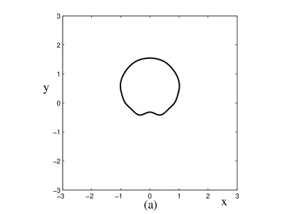
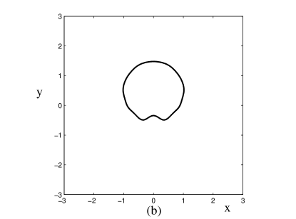
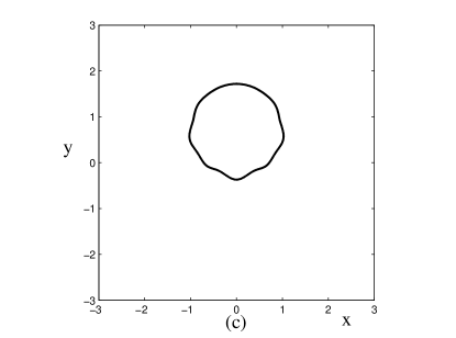
A basic numerical code using MATLAB was developed to simulate some simple cases, in all of which the patch has zero vorticity. This allowed us to compare our results with that of Baker and Mooreโ€™s simulations for the evolution of an initially circular patch with zero vorticity, and we chose the same parameter values $\rho_{o}=1,\rho_{i}=0$ and $g=1$ [4]. It may be recalled that their motivation was to simulate the experimentally observed phenomenon of a jet forming in the rear of an almost planar buoyant gas bubble. We also considered two cases in which the initial shape is an ellipse of small eccentricity. In all the three cases, the shapes are initially symmetric about the $y$-axis and consequently maintain this symmetry during evolution. Therefore, we solve only for the left side and obtain the right side by symmetry. As described above, in our method we have to solve the coupled system (11) and (LABEL:eq:sheetevol), while updating the boundary at each time step using (10). Since the centroid moves only in the vertical direction, $V_{c}$ is viewed as a scalar, and the sheet strength is discretised as $\gamma_{\mathfrak{s}}=\sum_{n=1}^{N}f_{n}(t)\sin n\theta$, where $\theta\in[0,\pi]$ is reckoned positive counterclockwise from the positive $y$-axis.

We need a system of $(N+1)$ ODEs for the $(N+1)$ time dependent unknowns $V_{c},f_{i},i=1,...N$. The first of these is generated by plugging in the forms of $V_{c}$ and ฮณssubscript๐›พ๐‘ \gamma_{s} into (11); it is seen that the horizontal components vanish. The remaining $N$ equations of the ODE system are obtained by plugging the forms of $V_{c}$ and $\gamma_{\mathfrak{s}}$ into (LABEL:eq:sheetevol) which yields an expression of the form $\sum_{n=1}^{N}C_{n}(dV_{c}/dt,d\gamma_{\mathfrak{s}}/dt)\sin n\theta=0$, where the $C_{n}$ are linear in the unknowns; for simplicity, we have not displayed the $C_{n}$. This is possible only if $C_{n}=0$ for $n=1,...N$ and leads to the remaining $N$ ODEs.

Denoting the vector $u={V_{c},f_{1},..f_{N}}$, the ODE system is finally written as $Adu/dt=B$, which is then integrated by a simple first order Euler time stepping. Updating the boundary position of the boundary via (10) is also by Euler time stepping. Computations can be continued till a time the patch boundary remains single valued in $\theta$. Results are presented in Figure 2 for three different cases of initial conditions- (a) circular boundary with $\gamma_{\mathfrak{s}}=10^{-5}\sin\theta$, (b) elliptic boundary with semi-major and semi-minor axes $a=1.001,b=1.$ with $\gamma_{\mathfrak{s}}=0$ and (c) elliptic boundary with $a=1,b=1.001$ with $\gamma_{\mathfrak{s}}=0$. 100 boundary points and 10 fourier modes were used in the computation. For the Baker and Moore case, Figure 2 (a), a dimple suggesting an incipient jet formation is observed. However, as soon as folds develop numerical instability sets in. The comparison with [4] was therefore mostly inconclusive.

The procedure is similar for non-zero patch vorticity. However, there will in general be no symmetry and the full fourier series for ฮณssubscript๐›พ๐‘ \gamma_{s} will have to be used. The centroid vorticity will have two components $V_{cx}$ and $V_{cy}$.

Refer to caption
Refer to caption
Refer to caption
Figure 2: Evolution of the patch boundary, separating fluids of densities $\rho_{o}=1$ and $\rho_{i}=0$ with different initial conditions. At time $t=0$ the centroid of the bubble is at $x=y=0$. Acceleration due to gravity $g=1.$ (a) Initially circular boundary with ฮณs=10โˆ’5โ€‹sinโกฮธsubscript๐›พ๐‘ superscript105๐œƒ\gamma_{s}=10^{-5}\sin\theta, at $t=1.08,$ (b) initially elliptic boundary with a=1.001,b=1,ฮณs=0formulae-sequence๐‘Ž1.001formulae-sequence๐‘1subscript๐›พ๐‘ 0a=1.001,b=1,\gamma_{s}=0, at $t=1.02$ and (c) initially elliptic boundary with a=1,b=1.001,ฮณs=0formulae-sequence๐‘Ž1formulae-sequence๐‘1.001subscript๐›พ๐‘ 0a=1,b=1.001,\gamma_{s}=0, at $t=1.20$. Note the incipient upward jet in the first two cases.

4.1 Small buoyant patches and buoyant point vortices

In the limit of vanishing patch size, the equations derived in the previous sections should lead to the equation governing an isolated buoyant point vortex and thereby to the equations governing interacting buoyant point vortices. For $\epsilon$ patches (small buoyant patches of characteristic length $\epsilon$), and especially in the limit of vanishing size, equationsย (10) andย (LABEL:eq:sheetevol) are irrelevant.

Examiningย (11) in the limit of $\epsilon\rightarrow 0$, it is reasonable to assume that the sheet strength $\gamma_{\mathfrak{s}}$, and all other slip velocity fields, go to zero whereas $\omega\rightarrow\infty$ such that ฯ‰โ€‹A=cโ€‹oโ€‹nโ€‹sโ€‹tโ€‹aโ€‹nโ€‹t=ฮ“o๐œ”๐ด๐‘๐‘œ๐‘›๐‘ ๐‘ก๐‘Ž๐‘›๐‘กsubscriptฮ“๐‘œ\omega A=constant=\Gamma_{o}. One can write $\Psi_{i}\mid_{\bar{C}}=\Psi_{i}(0)+O(1)$, where $\Psi_{i}(0)=O(\log\epsilon)$ is the value at the centroid and corresponds to the value for a point vortex. It follows that โˆฎCยฏฮจiโ€‹t^โ€‹๐‘‘s=Oโ€‹(ฯต2)subscriptcontour-integralยฏ๐ถsubscriptฮจ๐‘–^๐‘กdifferential-d๐‘ ๐‘‚superscriptitalic-ฯต2\oint_{\bar{C}}\Psi_{i}\hat{t}\;ds=O(\epsilon^{2}), and โˆฎCยฏฮณโ€‹lโ€‹๐‘‘ssubscriptcontour-integralยฏ๐ถ๐›พ๐‘™differential-d๐‘ \oint_{\bar{C}}\gamma l\;ds goes to zero even faster. The time scale in the limit should correspond to that of the centroid motion, i.e. $O(1)$, and so the time derivatives of these integrals should be of the same order as the integrals. We now distinguish two possibilities.

  • โ€ข

    ฯiโ†’โˆžโ†’subscript๐œŒ๐‘–\rho_{i}\rightarrow\infty such that ฯiโ€‹A=cโ€‹oโ€‹nโ€‹sโ€‹tโ€‹aโ€‹nโ€‹tsubscript๐œŒ๐‘–๐ด๐‘๐‘œ๐‘›๐‘ ๐‘ก๐‘Ž๐‘›๐‘ก\rho_{i}A=constant where $A=O(\epsilon^{2}).$ This is the so-called massive point vortex [13]. In this limit, the integrals with $\rho_{o}$ as coefficient are negligible, being $O(\epsilon^{2})$. However, conistent with the above estimates, the term consisting of the integral involving $\Psi_{i}$, with $\rho_{i}$ as coefficient, is $O(1)$, which renders it non-negligible. The dynamics of the point vortex is governed by a second-order differential equation in its position coordinates, involving the gyroscopic Kutta lift and the weight of the vortex. Motion of the point vortex in this case is possible.

  • โ€ข

    ฯi=cโ€‹oโ€‹nโ€‹sโ€‹t.subscript๐œŒ๐‘–๐‘๐‘œ๐‘›๐‘ ๐‘ก\rho_{i}=const. This is the classical point vortex system, valid for homogeneous fluid. The dynamics is governed by the well-known standard first order ODE system, and the vortex will remain at rest.

Glass et al [13] examined the limiting dynamics when a rigid body with fixed circulation shrinks to a point and highlighted that this limit leads to a singular perturbation problem which has to correctly analysed. They purport to provide such an analysis and demonstrate the above mentioned two distinguished limits of the massive and classical point vortices. A particularly interesting aspect of the problem is the dependence of the singularities on the symmetry of the shrinking body and their detailed treatment. A similar detailed analysis for the present model may be required to obtain the correct buoyant point vortex equations. For another perspective on point vortices with mass, see [15].

5 Concluding remarks

The evolution of a two-dimensional buoyant vortex patch is studied by a clear and detailed momentum analysis of its motion. Framing the motion as being due to motion of the patch centroid and a deformation results in a rational derivation of equations of motion for the centroid and the patch boundary. It is seen that the centroid motion depends on the internal flow in the patch as well as the patch shape. A similar, but simpler, equation for a vortex with a finite, but small, buoyant circular core, was given (eq. A4, [29]) in an ad hoc manner; core deformation and velocity variations in the core were neglected. Ravichandran et al (2017) [28] also write an ad hoc equation for the centroid of a buoyant Rankine vortex which is incorrect in fundamental ways, with even the apparent mass term $\rho_{o}dV_{c}/dt$ omitted; the effect of the vortex sheet and its deformation is anyway not included. This leads to the incorrect claim (eq.(5) of [28]) that a Rankine vortex, i.e. a patch of circular shape, translates at constant speed for any density ratio; this is in direct contradiction of the results obtained in [17] and in this paper. In fact, the equation purportedly describing the motion of the vortex centroid, eq.(3) in [28], is really a description of that of a buoyant rigid cylinder with non-zero circulation.

The present analysis, from first principles, demonstrates conclusively the effects of the added mass and the deformation of the vortex patch โ€“due to the patch vorticity and the essential slip field resulting from enforcing pressure continuityโ€“ on the motion of the centroid. The analysis is facilitated by splitting the velocity field into ones due to the vortex patch, a bounding vortex sheet and the internal and external Kirchhoff flows generated by the translation of the instantaneous patch shape. This decomposition lays bare the physical causal chain, which can be summarised as a) the velocity fields due to the patch and bounding vortex sheet causing a change in shape of the patch given byย (10), which then, by ย (11) andย (LABEL:eq:sheetevol), (b) leads to a change of the sheet strength distribution ฮณssubscript๐›พ๐‘ \gamma_{s} and the centroid velocity $V_{c}$ which then (c) changes the patch shape (again throughย (10)). Even though the evolution equations for ฮณssubscript๐›พ๐‘ \gamma_{s} and $V_{c}$ appear to be coupled in a complicated manner, it turns out to be possible to express $dV_{c}/dt$ in terms of โˆ‚ฮณs/โˆ‚tsubscript๐›พ๐‘ ๐‘ก\partial\gamma_{s}/\partial t and $dl/dt.$ The decoupling allows the computation of the patch shape, sheet strength and centroid velocity in that order. The analysis also reveals that the point vortex limit should be carefully carried out. Another interesting direction would be to construct a Hamiltonian model of interacting buoyant patches, along the lines of [23].

Appendix A

The momentum theorem applied to the fluid in $D_{R}$, at a given time $t$, gives

$\displaystyle\rho_{i}\frac{d}{dt}\int_{D_{v}(t)}v\;dA+\rho_{o}\frac{d}{dt}\int_{\tilde{D}(t)}v\;dA$ =โˆ’โˆฎCRpโ€‹n^โ€‹๐‘‘sโˆ’(ฯiโ€‹Aโ€‹g+ฯoโ€‹(ฯ€โ€‹R2โˆ’A)โ€‹g)โ€‹j^,absentsubscriptcontour-integralsubscript๐ถ๐‘…๐‘^๐‘›differential-d๐‘ subscript๐œŒ๐‘–๐ด๐‘”subscript๐œŒ๐‘œ๐œ‹superscript๐‘…2๐ด๐‘”^๐‘—\displaystyle=-\oint_{C_{R}}p\hat{n}\;ds-\left(\rho_{i}Ag+\rho_{o}(\pi R^{2}-A)g\right)\hat{j},

Now, use the vector identity valid for any vector field $a$ in a domain $\mathfrak{D}\subset\mathbb{R}^{2}$,

$\displaystyle\int_{\mathfrak{D}}a\;dA$ =โˆซ๐”‡rร—(โˆ‡ร—a)โ€‹๐‘‘Aโˆ’โˆฎโˆ‚๐”‡rร—(n^ร—a)โ€‹๐‘‘sabsentsubscript๐”‡๐‘Ÿโˆ‡๐‘Ždifferential-d๐ดsubscriptcontour-integral๐”‡๐‘Ÿ^๐‘›๐‘Ždifferential-d๐‘ \displaystyle=\int_{\mathfrak{D}}r\times(\nabla\times a)\;dA-\oint_{\partial\mathfrak{D}}r\times\left(\hat{n}\times a\right)\;ds (A1)

to write the momentum theorem as

ฯiโ€‹ddโ€‹tโ€‹(โˆซDvโ€‹(t)rร—ฯ‰โ€‹k^โ€‹๐‘‘Aโˆ’โˆฎโˆ‚Dvโ€‹(t)rร—(n^ร—vi)โ€‹๐‘‘s)subscript๐œŒ๐‘–๐‘‘๐‘‘๐‘กsubscriptsubscript๐ท๐‘ฃ๐‘ก๐‘Ÿ๐œ”^๐‘˜differential-d๐ดsubscriptcontour-integralsubscript๐ท๐‘ฃ๐‘ก๐‘Ÿ^๐‘›subscript๐‘ฃ๐‘–differential-d๐‘ \displaystyle\rho_{i}\frac{d}{dt}\left(\int_{D_{v}(t)}r\times\omega\hat{k}\;dA-\oint_{\partial D_{v}(t)}r\times\left(\hat{n}\times v_{i}\right)\;ds\right)
+ฯoโ€‹ddโ€‹tโ€‹(โˆซDโ€‹(t)rร—ฯ‰โ€‹k^โ€‹๐‘‘A+โˆฎโˆ‚Dvโ€‹(t)rร—(n^ร—vo)โ€‹๐‘‘sโˆ’โˆฎCRrร—(n^ร—vo)โ€‹๐‘‘s)subscript๐œŒ๐‘œ๐‘‘๐‘‘๐‘กsubscript๐ท๐‘ก๐‘Ÿ๐œ”^๐‘˜differential-d๐ดsubscriptcontour-integralsubscript๐ท๐‘ฃ๐‘ก๐‘Ÿ^๐‘›subscript๐‘ฃ๐‘œdifferential-d๐‘ subscriptcontour-integralsubscript๐ถ๐‘…๐‘Ÿ^๐‘›subscript๐‘ฃ๐‘œdifferential-d๐‘ \displaystyle+\rho_{o}\frac{d}{dt}\left(\int_{D(t)}r\times\omega\hat{k}\;dA+\oint_{\partial D_{v}(t)}r\times\left(\hat{n}\times v_{o}\right)\;ds-\oint_{C_{R}}r\times\left(\hat{n}\times v_{o}\right)\;ds\right)
=โˆ’โˆฎCRpโ€‹n^โ€‹๐‘‘sโˆ’(ฯiโ€‹Aโ€‹g+ฯoโ€‹(ฯ€โ€‹R2โˆ’A)โ€‹g)โ€‹j^,absentsubscriptcontour-integralsubscript๐ถ๐‘…๐‘^๐‘›differential-d๐‘ subscript๐œŒ๐‘–๐ด๐‘”subscript๐œŒ๐‘œ๐œ‹superscript๐‘…2๐ด๐‘”^๐‘—\displaystyle\hskip 144.54pt=-\oint_{C_{R}}p\hat{n}\;ds-\left(\rho_{i}Ag+\rho_{o}(\pi R^{2}-A)g\right)\hat{j},
$\displaystyle\Rightarrow$ ฯiโ€‹ddโ€‹tโ€‹โˆซDvโ€‹(t)rร—ฯ‰โ€‹k^โ€‹๐‘‘A+ฯoโ€‹ddโ€‹tโ€‹โˆฎโˆ‚Dvโ€‹(t)rร—(n^ร—vo)โ€‹๐‘‘sโˆ’ฯiโ€‹ddโ€‹tโ€‹โˆฎโˆ‚Dvโ€‹(t)rร—(n^ร—vi)โ€‹๐‘‘ssubscript๐œŒ๐‘–๐‘‘๐‘‘๐‘กsubscriptsubscript๐ท๐‘ฃ๐‘ก๐‘Ÿ๐œ”^๐‘˜differential-d๐ดsubscript๐œŒ๐‘œ๐‘‘๐‘‘๐‘กsubscriptcontour-integralsubscript๐ท๐‘ฃ๐‘ก๐‘Ÿ^๐‘›subscript๐‘ฃ๐‘œdifferential-d๐‘ subscript๐œŒ๐‘–๐‘‘๐‘‘๐‘กsubscriptcontour-integralsubscript๐ท๐‘ฃ๐‘ก๐‘Ÿ^๐‘›subscript๐‘ฃ๐‘–differential-d๐‘ \displaystyle\rho_{i}\frac{d}{dt}\int_{D_{v}(t)}r\times\omega\hat{k}\;dA+\rho_{o}\frac{d}{dt}\oint_{\partial D_{v}(t)}r\times\left(\hat{n}\times v_{o}\right)\;ds-\rho_{i}\frac{d}{dt}\oint_{\partial D_{v}(t)}r\times\left(\hat{n}\times v_{i}\right)\;ds
=ฯoโ€‹ddโ€‹tโ€‹โˆฎCRrร—(n^ร—vo)โ€‹๐‘‘sโˆ’โˆฎCRpโ€‹n^โ€‹๐‘‘sโˆ’(ฯiโ€‹Aโ€‹g+ฯoโ€‹(ฯ€โ€‹R2โˆ’A)โ€‹g)โ€‹j^,absentsubscript๐œŒ๐‘œ๐‘‘๐‘‘๐‘กsubscriptcontour-integralsubscript๐ถ๐‘…๐‘Ÿ^๐‘›subscript๐‘ฃ๐‘œdifferential-d๐‘ subscriptcontour-integralsubscript๐ถ๐‘…๐‘^๐‘›differential-d๐‘ subscript๐œŒ๐‘–๐ด๐‘”subscript๐œŒ๐‘œ๐œ‹superscript๐‘…2๐ด๐‘”^๐‘—\displaystyle\hskip 72.26999pt=\rho_{o}\frac{d}{dt}\oint_{C_{R}}r\times\left(\hat{n}\times v_{o}\right)\;ds-\oint_{C_{R}}p\hat{n}\;ds-\left(\rho_{i}Ag+\rho_{o}(\pi R^{2}-A)g\right)\hat{j},
$\displaystyle\Rightarrow$ ฯiโ€‹ddโ€‹tโ€‹โˆซDvโ€‹(t)(bcโ€‹(t)+l)ร—ฯ‰โ€‹k^โ€‹๐‘‘A+ฯoโ€‹ddโ€‹tโ€‹โˆฎโˆ‚Dvโ€‹(t)(bcโ€‹(t)+l)ร—(n^ร—vo)โ€‹๐‘‘ssubscript๐œŒ๐‘–๐‘‘๐‘‘๐‘กsubscriptsubscript๐ท๐‘ฃ๐‘กsubscript๐‘๐‘๐‘ก๐‘™๐œ”^๐‘˜differential-d๐ดsubscript๐œŒ๐‘œ๐‘‘๐‘‘๐‘กsubscriptcontour-integralsubscript๐ท๐‘ฃ๐‘กsubscript๐‘๐‘๐‘ก๐‘™^๐‘›subscript๐‘ฃ๐‘œdifferential-d๐‘ \displaystyle\rho_{i}\frac{d}{dt}\int_{D_{v}(t)}(b_{c}(t)+l)\times\omega\hat{k}\;dA+\rho_{o}\frac{d}{dt}\oint_{\partial D_{v}(t)}(b_{c}(t)+l)\times\left(\hat{n}\times v_{o}\right)\;ds
โˆ’ฯiโ€‹ddโ€‹tโ€‹โˆฎโˆ‚Dvโ€‹(t)(bcโ€‹(t)+l)ร—(n^ร—vi)โ€‹๐‘‘ssubscript๐œŒ๐‘–๐‘‘๐‘‘๐‘กsubscriptcontour-integralsubscript๐ท๐‘ฃ๐‘กsubscript๐‘๐‘๐‘ก๐‘™^๐‘›subscript๐‘ฃ๐‘–differential-d๐‘ \displaystyle\hskip 50.58878pt-\rho_{i}\frac{d}{dt}\oint_{\partial D_{v}(t)}(b_{c}(t)+l)\times\left(\hat{n}\times v_{i}\right)\;ds
=ฯoโ€‹ddโ€‹tโ€‹โˆฎCRrร—(n^ร—vo)โ€‹๐‘‘sโˆ’โˆฎCRpโ€‹n^โ€‹๐‘‘sโˆ’(ฯiโ€‹Aโ€‹g+ฯoโ€‹(ฯ€โ€‹R2โˆ’A)โ€‹g)โ€‹j^absentsubscript๐œŒ๐‘œ๐‘‘๐‘‘๐‘กsubscriptcontour-integralsubscript๐ถ๐‘…๐‘Ÿ^๐‘›subscript๐‘ฃ๐‘œdifferential-d๐‘ subscriptcontour-integralsubscript๐ถ๐‘…๐‘^๐‘›differential-d๐‘ subscript๐œŒ๐‘–๐ด๐‘”subscript๐œŒ๐‘œ๐œ‹superscript๐‘…2๐ด๐‘”^๐‘—\displaystyle\hskip 86.72377pt=\rho_{o}\frac{d}{dt}\oint_{C_{R}}r\times\left(\hat{n}\times v_{o}\right)\;ds-\oint_{C_{R}}p\hat{n}\;ds-\left(\rho_{i}Ag+\rho_{o}(\pi R^{2}-A)g\right)\hat{j}

Noting that, in general, for a velocity field on any closed curve $C$

โˆฎโˆ‚Cn^ร—vโ€‹๐‘‘s=ฮ“โ€‹k^,subscriptcontour-integral๐ถ^๐‘›๐‘ฃdifferential-d๐‘ ฮ“^๐‘˜\oint_{\partial C}\hat{n}\times v\;ds=\Gamma\hat{k},

where $\Gamma$ is the circulation, obtain

Vcร—ฯoโ€‹ฮ“oโ€‹k^+ฯoโ€‹ddโ€‹tโ€‹โˆฎโˆ‚Dvโ€‹(t)lร—(n^vร—vo)โ€‹๐‘‘sโˆ’ฯiโ€‹ddโ€‹tโ€‹โˆฎโˆ‚Dvโ€‹(t)lร—(n^vร—vi)โ€‹๐‘‘ssubscript๐‘‰๐‘subscript๐œŒ๐‘œsubscriptฮ“๐‘œ^๐‘˜subscript๐œŒ๐‘œ๐‘‘๐‘‘๐‘กsubscriptcontour-integralsubscript๐ท๐‘ฃ๐‘ก๐‘™subscript^๐‘›๐‘ฃsubscript๐‘ฃ๐‘œdifferential-d๐‘ subscript๐œŒ๐‘–๐‘‘๐‘‘๐‘กsubscriptcontour-integralsubscript๐ท๐‘ฃ๐‘ก๐‘™subscript^๐‘›๐‘ฃsubscript๐‘ฃ๐‘–differential-d๐‘ \displaystyle V_{c}\times\rho_{o}\Gamma_{o}\hat{k}+\rho_{o}\frac{d}{dt}\oint_{\partial D_{v}(t)}l\times\left(\hat{n}_{v}\times v_{o}\right)\;ds-\rho_{i}\frac{d}{dt}\oint_{\partial D_{v}(t)}l\times\left(\hat{n}_{v}\times v_{i}\right)\;ds
=ฯoโ€‹ddโ€‹tโ€‹โˆฎCRrร—(n^ร—vo)โ€‹๐‘‘sโˆ’โˆฎCRpโ€‹n^โ€‹๐‘‘sโˆ’((ฯiโˆ’ฯo)โ€‹A+ฯoโ€‹ฯ€โ€‹R2)โ€‹gโ€‹j^,absentsubscript๐œŒ๐‘œ๐‘‘๐‘‘๐‘กsubscriptcontour-integralsubscript๐ถ๐‘…๐‘Ÿ^๐‘›subscript๐‘ฃ๐‘œdifferential-d๐‘ subscriptcontour-integralsubscript๐ถ๐‘…๐‘^๐‘›differential-d๐‘ subscript๐œŒ๐‘–subscript๐œŒ๐‘œ๐ดsubscript๐œŒ๐‘œ๐œ‹superscript๐‘…2๐‘”^๐‘—\displaystyle\hskip 72.26999pt=\rho_{o}\frac{d}{dt}\oint_{C_{R}}r\times\left(\hat{n}\times v_{o}\right)\;ds-\oint_{C_{R}}p\hat{n}\;ds-\left((\rho_{i}-\rho_{o})A+\rho_{o}\pi R^{2}\right)g\hat{j},

where

$$V_{c}=\frac{db_{c}}{dt},$$

and $\Gamma_{o}$ is the constant circulation associated with the outside fluid (see Sections 2 and 3). Now use Bernoulliโ€™s on $C_{R}$,

$$p=-\rho_{o}\left(gy+\frac{\partial\phi}{\partial t}+\frac{1}{2}\nabla\phi\cdot\nabla\phi\right)+p_{\infty},$$

where $y$ is measured with respect to some datum and $p_{\infty}$ is a reference pressure. Evaluating just the gravity term,

ฯoโ€‹gโ€‹โˆฎCRyโ€‹n^โ€‹๐‘‘ssubscript๐œŒ๐‘œ๐‘”subscriptcontour-integralsubscript๐ถ๐‘…๐‘ฆ^๐‘›differential-d๐‘ \displaystyle\rho_{o}g\oint_{C_{R}}y\hat{n}\;ds $\displaystyle=\rho_{o}g\int_{D}\nabla y\;dA=\rho_{o}g\pi R^{2}\hat{k}$

The momentum equation now reads

Vcร—ฯoโ€‹ฮ“oโ€‹k^+ฯoโ€‹ddโ€‹tโ€‹โˆฎโˆ‚Dvโ€‹(t)lร—(n^vร—vo)โ€‹๐‘‘sโˆ’ฯiโ€‹ddโ€‹tโ€‹โˆฎโˆ‚Dvโ€‹(t)lร—(n^vร—vi)โ€‹๐‘‘ssubscript๐‘‰๐‘subscript๐œŒ๐‘œsubscriptฮ“๐‘œ^๐‘˜subscript๐œŒ๐‘œ๐‘‘๐‘‘๐‘กsubscriptcontour-integralsubscript๐ท๐‘ฃ๐‘ก๐‘™subscript^๐‘›๐‘ฃsubscript๐‘ฃ๐‘œdifferential-d๐‘ subscript๐œŒ๐‘–๐‘‘๐‘‘๐‘กsubscriptcontour-integralsubscript๐ท๐‘ฃ๐‘ก๐‘™subscript^๐‘›๐‘ฃsubscript๐‘ฃ๐‘–differential-d๐‘ \displaystyle V_{c}\times\rho_{o}\Gamma_{o}\hat{k}+\rho_{o}\frac{d}{dt}\oint_{\partial D_{v}(t)}l\times\left(\hat{n}_{v}\times v_{o}\right)\;ds-\rho_{i}\frac{d}{dt}\oint_{\partial D_{v}(t)}l\times\left(\hat{n}_{v}\times v_{i}\right)\;ds
=(ฯoโˆ’ฯi)โ€‹Aโ€‹gโ€‹j^+ฯoโ€‹ddโ€‹tโ€‹โˆฎCRrร—(n^ร—vo)โ€‹๐‘‘s+ฯoโ€‹โˆฎCR(โˆ‚ฯ•โˆ‚t+12โ€‹โˆ‡ฯ•โ‹…โˆ‡ฯ•)โ€‹n^โ€‹๐‘‘sabsentsubscript๐œŒ๐‘œsubscript๐œŒ๐‘–๐ด๐‘”^๐‘—subscript๐œŒ๐‘œ๐‘‘๐‘‘๐‘กsubscriptcontour-integralsubscript๐ถ๐‘…๐‘Ÿ^๐‘›subscript๐‘ฃ๐‘œdifferential-d๐‘ subscript๐œŒ๐‘œsubscriptcontour-integralsubscript๐ถ๐‘…italic-ฯ•๐‘กโ‹…12โˆ‡italic-ฯ•โˆ‡italic-ฯ•^๐‘›differential-d๐‘ \displaystyle\hskip 72.26999pt=(\rho_{o}-\rho_{i})Ag\hat{j}+\rho_{o}\frac{d}{dt}\oint_{C_{R}}r\times\left(\hat{n}\times v_{o}\right)\;ds+\rho_{o}\oint_{C_{R}}\left(\frac{\partial\phi}{\partial t}+\frac{1}{2}\nabla\phi\cdot\nabla\phi\right)\hat{n}\;ds

Far-field terms.

The next step is to show that all the $C_{R}$ contour integral terms go to zero as $R\rightarrow\infty$. If ฮ“oโ‰ 0subscriptฮ“๐‘œ0\Gamma_{o}\neq 0, $\phi_{o}$ is multiple-valued and the decay rates are given by

$$\phi_{o}(r,\theta)\sim\Gamma_{o}\theta,\>\theta=\tan^{-1}\left(\frac{y-y_{c}}{x-x_{c}}\right)\Rightarrow v_{o}(r,\theta)=\nabla\phi_{o}(r,\theta)\sim\frac{\Gamma_{o}}{r},\quad r\rightarrow\infty.$$

If $\Gamma_{o}=0$, then the decay rates are one order faster. The integral term containing $\nabla\phi\cdot\nabla\phi$ goes to zero from the far-field behavior (in either case). Next, use another vector identity

โˆฎCRrร—(n^ร—v)โ€‹๐‘‘s=โˆ’โˆฎCRฯ•โ€‹n^โ€‹๐‘‘s,subscriptcontour-integralsubscript๐ถ๐‘…๐‘Ÿ^๐‘›๐‘ฃdifferential-d๐‘ subscriptcontour-integralsubscript๐ถ๐‘…italic-ฯ•^๐‘›differential-d๐‘ \oint_{C_{R}}r\times\left(\hat{n}\times v\right)\;ds=-\oint_{C_{R}}\phi\hat{n}\;ds,

from which it is easily seen that the remaining integral terms on $C_{R}$ cancel leading to the final linear momentum balance equation

Vcร—ฯoโ€‹ฮ“oโ€‹k^+ฯoโ€‹ddโ€‹tโ€‹โˆฎโˆ‚Dvโ€‹(t)lร—(n^vร—vo)โ€‹๐‘‘ssubscript๐‘‰๐‘subscript๐œŒ๐‘œsubscriptฮ“๐‘œ^๐‘˜subscript๐œŒ๐‘œ๐‘‘๐‘‘๐‘กsubscriptcontour-integralsubscript๐ท๐‘ฃ๐‘ก๐‘™subscript^๐‘›๐‘ฃsubscript๐‘ฃ๐‘œdifferential-d๐‘ \displaystyle V_{c}\times\rho_{o}\Gamma_{o}\hat{k}+\rho_{o}\frac{d}{dt}\oint_{\partial D_{v}(t)}l\times\left(\hat{n}_{v}\times v_{o}\right)\;ds
โˆ’ฯiโ€‹ddโ€‹tโ€‹โˆฎโˆ‚Dvโ€‹(t)lร—(n^vร—vi)โ€‹๐‘‘s=(ฯoโˆ’ฯi)โ€‹Aโ€‹gโ€‹j^subscript๐œŒ๐‘–๐‘‘๐‘‘๐‘กsubscriptcontour-integralsubscript๐ท๐‘ฃ๐‘ก๐‘™subscript^๐‘›๐‘ฃsubscript๐‘ฃ๐‘–differential-d๐‘ subscript๐œŒ๐‘œsubscript๐œŒ๐‘–๐ด๐‘”^๐‘—\displaystyle\hskip 72.26999pt-\rho_{i}\frac{d}{dt}\oint_{\partial D_{v}(t)}l\times\left(\hat{n}_{v}\times v_{i}\right)\;ds=(\rho_{o}-\rho_{i})Ag\hat{j}

Appendix B

Noting that the $\nabla$ operator, in the respective coordinates, has the same form in the spatially-fixed and the centroid-fixed frames, the following relations hold

$$v_{i}=J\nabla\psi_{i}(r,t)=J\nabla\tilde{\psi}_{i}(l,t)=J\nabla\psi_{i}(l,t)$$

All the velocity decompositions and the velocity expressions in Section 3 continue to hold with the position vectors $r,\tilde{r}$ replaced by $l,\tilde{l}$. Moreover, the curve evolution in the two frames obeys the relation

$\displaystyle\frac{\partial C}{\partial t}$ $\displaystyle=\frac{\partial\bar{C}}{\partial t}+V_{c}\cdot\hat{n}_{\mid_{\bar{C}}}$

so that the curve evolution equation in the translating frame becomes

$\displaystyle\frac{\partial\bar{C}}{\partial t}$ $\displaystyle=\left(J\nabla\psi_{i}-V_{c}\right)\cdot\hat{n}_{\mid_{\bar{C}}}.$

This equation can also be written as

$\displaystyle\frac{\partial\bar{C}}{\partial t}$ $\displaystyle=J\nabla\Psi_{i}\cdot\hat{n}_{\mid_{\bar{C}}}=\bar{v}_{i}\cdot\hat{n}_{\mid_{\bar{C}}},$ (B1)

where

$\displaystyle\Psi_{i}(l,t)$ =ฯ‰2โ€‹ฯ€โ€‹โˆซDvโ€‹(t)logโกโˆฃlโˆ’l~โˆฃโ€‹dโ€‹A~+12โ€‹ฯ€โ€‹โˆฎCยฏฮณ๐”ฐโ€‹(s~,t)โ€‹logโกโˆฃlโˆ’l~โˆฃโ€‹dโ€‹s~absent๐œ”2๐œ‹subscriptsubscript๐ท๐‘ฃ๐‘กdelimited-โˆฃโˆฃ๐‘™~๐‘™๐‘‘~๐ด12๐œ‹subscriptcontour-integralยฏ๐ถsubscript๐›พ๐”ฐ~๐‘ ๐‘กdelimited-โˆฃโˆฃ๐‘™~๐‘™๐‘‘~๐‘ \displaystyle=\frac{\omega}{2\pi}\int_{D_{v}(t)}\log\mid l-\tilde{l}\mid\;d\tilde{A}+\frac{1}{2\pi}\oint_{\bar{C}}\gamma_{\mathfrak{s}}(\tilde{s},t)\log\mid l-\tilde{l}\mid\;d\tilde{s} (B2)

As for neutrally buoyant patches, using the standard theorems of integral calculus, the velocity field due to the patch can be written as a contour integral:

$\displaystyle J\nabla\left(\frac{\omega}{2\pi}\int_{D_{v}(t)}\log\mid l-\tilde{l}\mid\;d\tilde{A}\right)$ $\displaystyle=-\frac{\omega\hat{k}}{2\pi}\times\int_{D_{v}(t)}\nabla_{l}\log\mid l-\tilde{l}\mid\;d\tilde{A}$
=โˆ’ฯ‰โ€‹k^2โ€‹ฯ€ร—โˆฎCยฏlogโกโˆฃlโˆ’l~โˆฃโ€‹n^~โ€‹dโ€‹s~,absent๐œ”^๐‘˜2๐œ‹subscriptcontour-integralยฏ๐ถdelimited-โˆฃโˆฃ๐‘™~๐‘™~^๐‘›๐‘‘~๐‘ \displaystyle=-\frac{\omega\hat{k}}{2\pi}\times\oint_{\bar{C}}\log\mid l-\tilde{l}\mid\tilde{\hat{n}}\;d\tilde{s},
=โˆ’ฯ‰2โ€‹ฯ€โ€‹โˆฎCยฏlogโกโˆฃlโˆ’l~โˆฃโ€‹t^~โ€‹dโ€‹s~absent๐œ”2๐œ‹subscriptcontour-integralยฏ๐ถdelimited-โˆฃโˆฃ๐‘™~๐‘™~^๐‘ก๐‘‘~๐‘ \displaystyle=-\frac{\omega}{2\pi}\oint_{\bar{C}}\log\mid l-\tilde{l}\mid\tilde{\hat{t}}\;d\tilde{s}

This allows (B1) to be written in the contour integral form ย (10).

Appendix C

Let $v$ denote the Eulerian velocity fields, $V$ denote the material/Lagrangian velocities and $p$ the Eulerian pressure fields, with corresponding subscripts for inner and outer fluid. Denote by xโ€‹(s,t),yโ€‹(s,t)๐‘ฅ๐‘ ๐‘ก๐‘ฆ๐‘ ๐‘กx(s,t),y(s,t) the $\mathbb{R}^{2}$-coordinates of material points on the interface, where s๐‘ s is the interface curve parameter. From the equivalence of the Eulerian and Lagrangian descriptions,

vโ€‹(xโ€‹(s,t),yโ€‹(s,t))=Vโ€‹(s,t).๐‘ฃ๐‘ฅ๐‘ ๐‘ก๐‘ฆ๐‘ ๐‘ก๐‘‰๐‘ ๐‘กv(x(s,t),y(s,t))=V(s,t).

Let $g$ denote the gravity vector. Apply Eulerโ€™s equation at the interface for the inner and the outer fluid:

ฯiโ€‹Dโ€‹viDโ€‹tโ€‹(xโ€‹(s,t),yโ€‹(s,t))subscript๐œŒ๐‘–๐ทsubscript๐‘ฃ๐‘–๐ท๐‘ก๐‘ฅ๐‘ ๐‘ก๐‘ฆ๐‘ ๐‘ก\displaystyle\rho_{i}\frac{Dv_{i}}{Dt}(x(s,t),y(s,t)) =โˆ’โˆ‡piโ€‹(xโ€‹(s,t),yโ€‹(s,t))โˆ’ฯiโ€‹gโ€‹j^,absentโˆ‡subscript๐‘๐‘–๐‘ฅ๐‘ ๐‘ก๐‘ฆ๐‘ ๐‘กsubscript๐œŒ๐‘–๐‘”^๐‘—\displaystyle=-\nabla p_{i}(x(s,t),y(s,t))-\rho_{i}g\hat{j},
ฯoโ€‹Dโ€‹voDโ€‹tโ€‹(xโ€‹(s,t),yโ€‹(s,t))subscript๐œŒ๐‘œ๐ทsubscript๐‘ฃ๐‘œ๐ท๐‘ก๐‘ฅ๐‘ ๐‘ก๐‘ฆ๐‘ ๐‘ก\displaystyle\rho_{o}\frac{Dv_{o}}{Dt}(x(s,t),y(s,t)) =โˆ’โˆ‡poโ€‹(xโ€‹(s,t),yโ€‹(s,t))โˆ’ฯoโ€‹gโ€‹j^,absentโˆ‡subscript๐‘๐‘œ๐‘ฅ๐‘ ๐‘ก๐‘ฆ๐‘ ๐‘กsubscript๐œŒ๐‘œ๐‘”^๐‘—\displaystyle=-\nabla p_{o}(x(s,t),y(s,t))-\rho_{o}g\hat{j},

where all spatial derivatives are one-sided derivatives. If t^โ€‹(s,t)^๐‘ก๐‘ ๐‘ก\hat{t}(s,t) denotes the unit tangent field then

ฯiโ€‹(Dโ€‹viDโ€‹tโ‹…t^)โ€‹(xโ€‹(s,t),yโ€‹(s,t))subscript๐œŒ๐‘–โ‹…๐ทsubscript๐‘ฃ๐‘–๐ท๐‘ก^๐‘ก๐‘ฅ๐‘ ๐‘ก๐‘ฆ๐‘ ๐‘ก\displaystyle\rho_{i}\left(\frac{Dv_{i}}{Dt}\cdot\hat{t}\right)(x(s,t),y(s,t))
=โˆ’(โˆ‡piโ‹…t^)โ€‹(xโ€‹(s,t),yโ€‹(s,t))โˆ’ฯiโ€‹gโ€‹j^โ‹…t^โ€‹(xโ€‹(s,t),yโ€‹(s,t)),absentโˆ‡โ‹…subscript๐‘๐‘–^๐‘ก๐‘ฅ๐‘ ๐‘ก๐‘ฆ๐‘ ๐‘กโ‹…subscript๐œŒ๐‘–๐‘”^๐‘—^๐‘ก๐‘ฅ๐‘ ๐‘ก๐‘ฆ๐‘ ๐‘ก\displaystyle\hskip 72.26999pt=-\left(\nabla p_{i}\cdot\hat{t}\right)(x(s,t),y(s,t))-\rho_{i}g\hat{j}\cdot\hat{t}(x(s,t),y(s,t)),
ฯoโ€‹(Dโ€‹voDโ€‹tโ‹…t^)โ€‹(xโ€‹(s,t),yโ€‹(s,t))subscript๐œŒ๐‘œโ‹…๐ทsubscript๐‘ฃ๐‘œ๐ท๐‘ก^๐‘ก๐‘ฅ๐‘ ๐‘ก๐‘ฆ๐‘ ๐‘ก\displaystyle\rho_{o}\left(\frac{Dv_{o}}{Dt}\cdot\hat{t}\right)(x(s,t),y(s,t))
=โˆ’(โˆ‡poโ‹…t^)โ€‹(xโ€‹(s,t),yโ€‹(s,t))โˆ’ฯoโ€‹gโ€‹j^โ‹…t^โ€‹(xโ€‹(s,t),yโ€‹(s,t)),absentโˆ‡โ‹…subscript๐‘๐‘œ^๐‘ก๐‘ฅ๐‘ ๐‘ก๐‘ฆ๐‘ ๐‘กโ‹…subscript๐œŒ๐‘œ๐‘”^๐‘—^๐‘ก๐‘ฅ๐‘ ๐‘ก๐‘ฆ๐‘ ๐‘ก\displaystyle\hskip 72.26999pt=-\left(\nabla p_{o}\cdot\hat{t}\right)(x(s,t),y(s,t))-\rho_{o}g\hat{j}\cdot\hat{t}(x(s,t),y(s,t)),

Continuity of velocity.

If the velocity at the interface is continuous, then at each s๐‘ s

viโ€‹(xโ€‹(s,t),yโ€‹(s,t))=voโ€‹(xโ€‹(s,t),yโ€‹(s,t)),โˆ€tsubscript๐‘ฃ๐‘–๐‘ฅ๐‘ ๐‘ก๐‘ฆ๐‘ ๐‘กsubscript๐‘ฃ๐‘œ๐‘ฅ๐‘ ๐‘ก๐‘ฆ๐‘ ๐‘กfor-all๐‘กv_{i}(x(s,t),y(s,t))=v_{o}(x(s,t),y(s,t)),\quad\forall t

and, in the Lagrangian description,

Viโ€‹(s,t)=Voโ€‹(s,t),โˆ€tsubscript๐‘‰๐‘–๐‘ ๐‘กsubscript๐‘‰๐‘œ๐‘ ๐‘กfor-all๐‘กV_{i}(s,t)=V_{o}(s,t),\quad\forall t

From this equation, it follows that at each s๐‘ s,

dโ€‹Vidโ€‹tโ€‹(s,t)=dโ€‹Vodโ€‹tโ€‹(s,t),โˆ€t๐‘‘subscript๐‘‰๐‘–๐‘‘๐‘ก๐‘ ๐‘ก๐‘‘subscript๐‘‰๐‘œ๐‘‘๐‘ก๐‘ ๐‘กfor-all๐‘ก\frac{dV_{i}}{dt}(s,t)=\frac{dV_{o}}{dt}(s,t),\quad\forall t

Reverting to the Eulerian framework, the equivalence gives

Dโ€‹viDโ€‹tโ€‹(xโ€‹(s,t),yโ€‹(s,t))=Dโ€‹voDโ€‹tโ€‹(xโ€‹(s,t),yโ€‹(s,t)),โˆ€t๐ทsubscript๐‘ฃ๐‘–๐ท๐‘ก๐‘ฅ๐‘ ๐‘ก๐‘ฆ๐‘ ๐‘ก๐ทsubscript๐‘ฃ๐‘œ๐ท๐‘ก๐‘ฅ๐‘ ๐‘ก๐‘ฆ๐‘ ๐‘กfor-all๐‘ก\frac{Dv_{i}}{Dt}(x(s,t),y(s,t))=\frac{Dv_{o}}{Dt}(x(s,t),y(s,t)),\quad\forall t

Continuity of pressure.

If the pressure at the interface is continuous, then at each s๐‘ s

piโ€‹(xโ€‹(s,t),yโ€‹(s,t))subscript๐‘๐‘–๐‘ฅ๐‘ ๐‘ก๐‘ฆ๐‘ ๐‘ก\displaystyle p_{i}(x(s,t),y(s,t)) =poโ€‹(xโ€‹(s,t),yโ€‹(s,t)),โˆ€t,absentsubscript๐‘๐‘œ๐‘ฅ๐‘ ๐‘ก๐‘ฆ๐‘ ๐‘กfor-all๐‘ก\displaystyle=p_{o}(x(s,t),y(s,t)),\quad\forall t,
โ‡’Piโ€‹(s,t)โ‡’absentsubscript๐‘ƒ๐‘–๐‘ ๐‘ก\displaystyle\Rightarrow P_{i}(s,t) =Poโ€‹(s,t),โˆ€t,absentsubscript๐‘ƒ๐‘œ๐‘ ๐‘กfor-all๐‘ก\displaystyle=P_{o}(s,t),\quad\forall t,
โ‡’โˆ‚Piโˆ‚sโ‡’absentsubscript๐‘ƒ๐‘–๐‘ \displaystyle\Rightarrow\frac{\partial P_{i}}{\partial s} =โˆ‚Poโˆ‚s,โˆ€t,absentsubscript๐‘ƒ๐‘œ๐‘ for-all๐‘ก\displaystyle=\frac{\partial P_{o}}{\partial s},\quad\forall t,
โ‡’(โˆ‡piโ‹…t^)โ€‹(xโ€‹(s,t),yโ€‹(s,t))โ‡’absentโˆ‡โ‹…subscript๐‘๐‘–^๐‘ก๐‘ฅ๐‘ ๐‘ก๐‘ฆ๐‘ ๐‘ก\displaystyle\Rightarrow\left(\nabla p_{i}\cdot\hat{t}\right)(x(s,t),y(s,t)) =(โˆ‡poโ‹…t^)โ€‹(xโ€‹(s,t),yโ€‹(s,t)),โˆ€t,absentโˆ‡โ‹…subscript๐‘๐‘œ^๐‘ก๐‘ฅ๐‘ ๐‘ก๐‘ฆ๐‘ ๐‘กfor-all๐‘ก\displaystyle=\left(\nabla p_{o}\cdot\hat{t}\right)(x(s,t),y(s,t)),\quad\forall t,
Proposition 1

For a buoyant patch, pressure and velocity continuity at the interface cannot be simultaneously satisfied.

Proof
Proof by contradiction. If they can be simultaneously satisfied, then at the interface we have

(ฯiโˆ’ฯo)โ€‹(Dโ€‹viDโ€‹tโ‹…t^)โ€‹(xโ€‹(s,t),yโ€‹(s,t))subscript๐œŒ๐‘–subscript๐œŒ๐‘œโ‹…๐ทsubscript๐‘ฃ๐‘–๐ท๐‘ก^๐‘ก๐‘ฅ๐‘ ๐‘ก๐‘ฆ๐‘ ๐‘ก\displaystyle\left(\rho_{i}-\rho_{o}\right)\left(\frac{Dv_{i}}{Dt}\cdot\hat{t}\right)(x(s,t),y(s,t)) =โˆ’(ฯiโˆ’ฯo)โ€‹gโ€‹j^โ‹…t^โ€‹(xโ€‹(s,t),yโ€‹(s,t))absentโ‹…subscript๐œŒ๐‘–subscript๐œŒ๐‘œ๐‘”^๐‘—^๐‘ก๐‘ฅ๐‘ ๐‘ก๐‘ฆ๐‘ ๐‘ก\displaystyle=-\left(\rho_{i}-\rho_{o}\right)g\hat{j}\cdot\hat{t}(x(s,t),y(s,t))

There are only two ways in which this equation can be satisfied: (i) for a neutrally buoyant patch or (ii) if acceleration of interface elements is equal to $-g\hat{j}$ plus a normal component. The latter is impossible since it implies that the patch is free falling while at the same time interface elements are traveling at constant speeds around the interface (with a normal centripetal acceleration) โ– โ– \blacksquare

The conclusion is therefore one can choose to make either the pressure or the velocity continuous at the interface for a buoyant patch. Choosing one however implies a rule for the other, to satisfy Eulerโ€™s equation. With pressure continuity, the velocity at the interface must obey the following slip rule:

ฯiโ€‹(Dโ€‹viDโ€‹tโ‹…t^)โ€‹(xโ€‹(s,t),yโ€‹(s,t))โˆ’ฯoโ€‹(Dโ€‹voDโ€‹tโ‹…t^)โ€‹(xโ€‹(s,t),yโ€‹(s,t))subscript๐œŒ๐‘–โ‹…๐ทsubscript๐‘ฃ๐‘–๐ท๐‘ก^๐‘ก๐‘ฅ๐‘ ๐‘ก๐‘ฆ๐‘ ๐‘กsubscript๐œŒ๐‘œโ‹…๐ทsubscript๐‘ฃ๐‘œ๐ท๐‘ก^๐‘ก๐‘ฅ๐‘ ๐‘ก๐‘ฆ๐‘ ๐‘ก\displaystyle\rho_{i}\left(\frac{Dv_{i}}{Dt}\cdot\hat{t}\right)(x(s,t),y(s,t))-\rho_{o}\left(\frac{Dv_{o}}{Dt}\cdot\hat{t}\right)(x(s,t),y(s,t))
=(ฯoโˆ’ฯi)โ€‹gโ€‹j^โ‹…t^โ€‹(xโ€‹(s,t),yโ€‹(s,t))absentโ‹…subscript๐œŒ๐‘œsubscript๐œŒ๐‘–๐‘”^๐‘—^๐‘ก๐‘ฅ๐‘ ๐‘ก๐‘ฆ๐‘ ๐‘ก\displaystyle\hskip 144.54pt=\left(\rho_{o}-\rho_{i}\right)g\hat{j}\cdot\hat{t}(x(s,t),y(s,t))

This slip rule will affect the motion of the centroid and the motion of the interface as well.

Continuity of pressure is the commonly used dynamic boundary condition at surface-tension-free interfaces. Alternatively, one could argue that it is the force due to pressure that must be continuous. It is a basic fact that the force due to pressure is equal to $\nabla p(x,y)\delta\mathcal{V}$ for a material element of volume $\delta\mathcal{V}$ centered at point $(x,y)$.

Continuity of force per unit volume (due to pressure)

If the force per unit volume (due to pressure) at the interface is continuous, then at each s๐‘ s,

โˆ‡piโ€‹(xโ€‹(s,t),yโ€‹(s,t))โˆ‡subscript๐‘๐‘–๐‘ฅ๐‘ ๐‘ก๐‘ฆ๐‘ ๐‘ก\displaystyle\nabla p_{i}(x(s,t),y(s,t)) =โˆ‡poโ€‹(xโ€‹(s,t),yโ€‹(s,t)),โˆ€t,absentโˆ‡subscript๐‘๐‘œ๐‘ฅ๐‘ ๐‘ก๐‘ฆ๐‘ ๐‘กfor-all๐‘ก\displaystyle=\nabla p_{o}(x(s,t),y(s,t)),\quad\forall t,

It is easy to see that we then have a similar Proposition.

Proposition 2

For a buoyant patch, force per unit volume (due to pressure) and velocity continuity at the interface cannot be simultaneously satisfied.

With force( due to pressure) continuity, the velocity at the interface, both tangential and normal components, must obey the following stronger rule:

ฯiโ€‹Dโ€‹viDโ€‹tโ€‹(xโ€‹(s,t),yโ€‹(s,t))โˆ’ฯoโ€‹Dโ€‹voDโ€‹tโ€‹(xโ€‹(s,t),yโ€‹(s,t))subscript๐œŒ๐‘–๐ทsubscript๐‘ฃ๐‘–๐ท๐‘ก๐‘ฅ๐‘ ๐‘ก๐‘ฆ๐‘ ๐‘กsubscript๐œŒ๐‘œ๐ทsubscript๐‘ฃ๐‘œ๐ท๐‘ก๐‘ฅ๐‘ ๐‘ก๐‘ฆ๐‘ ๐‘ก\displaystyle\rho_{i}\frac{Dv_{i}}{Dt}(x(s,t),y(s,t))-\rho_{o}\frac{Dv_{o}}{Dt}(x(s,t),y(s,t)) =(ฯiโˆ’ฯo)โ€‹gโ€‹(xโ€‹(s,t),yโ€‹(s,t))absentsubscript๐œŒ๐‘–subscript๐œŒ๐‘œ๐‘”๐‘ฅ๐‘ ๐‘ก๐‘ฆ๐‘ ๐‘ก\displaystyle=\left(\rho_{i}-\rho_{o}\right)g(x(s,t),y(s,t))

Thus the equality of the gradient of pressure reveals another interesting possibility, due to taking one-sided derivatives. One can have equality of $\nabla p$ at the interface, yet the pressure itself could be discontinuous.

Appendix D

With s๐‘ s denoting the arc-length parameter, s๐‘ s and $t$ are independent variables, and we make the following identifications. For points on the boundary,

lโ‰กlโ€‹(s,t)โ‰กCยฏโ€‹(s,t),l~โ‰กlโ€‹(s~,t),t^โ‰กt^โ€‹(s,t),t^~โ‰กt^โ€‹(s~,t).formulae-sequence๐‘™๐‘™๐‘ ๐‘กยฏ๐ถ๐‘ ๐‘กformulae-sequence~๐‘™๐‘™~๐‘ ๐‘กformulae-sequence^๐‘ก^๐‘ก๐‘ ๐‘ก~^๐‘ก^๐‘ก~๐‘ ๐‘กl\equiv l(s,t)\equiv\bar{C}(s,t),\quad\tilde{l}\equiv l(\tilde{s},t),\quad\hat{t}\equiv\hat{t}(s,t),\quad\tilde{\hat{t}}\equiv\hat{t}(\tilde{s},t).

Moreover,

t^=โˆ‚Cยฏโˆ‚s^๐‘กยฏ๐ถ๐‘ \hat{t}=\frac{\partial\bar{C}}{\partial s}

The derivatives of the integral terms are now evaluated as follows:

ddโ€‹tโ€‹โˆฎCยฏฮจiโ€‹t^โ€‹๐‘‘s=โˆฎCยฏ(โˆ‚ฮจiโˆ‚tโ€‹t^+ฮจiโ€‹โˆ‚t^โˆ‚t)โ€‹๐‘‘s,๐‘‘๐‘‘๐‘กsubscriptcontour-integralยฏ๐ถsubscriptฮจ๐‘–^๐‘กdifferential-d๐‘ subscriptcontour-integralยฏ๐ถsubscriptฮจ๐‘–๐‘ก^๐‘กsubscriptฮจ๐‘–^๐‘ก๐‘กdifferential-d๐‘ \displaystyle\frac{d}{dt}\oint_{\bar{C}}\Psi_{i}\hat{t}\;ds=\oint_{\bar{C}}\left(\frac{\partial\Psi_{i}}{\partial t}\hat{t}+\Psi_{i}\frac{\partial\hat{t}}{\partial t}\right)\;ds,
$\displaystyle=\oint_{\bar{C}}\left(\frac{\omega\hat{t}}{2\pi}\frac{\partial l}{\partial t}\cdot\int_{D_{v}(t)}\frac{l-\tilde{l}}{\mid l-\tilde{l}\mid^{2}}\;d\tilde{A}+\oint_{\bar{C}}\frac{\hat{t}}{2\pi}\frac{\partial l}{\partial t}\cdot\oint_{\bar{C}}\gamma_{\mathfrak{s}}(\tilde{s},t)\frac{l-\tilde{l}}{\mid l-\tilde{l}\mid^{2}}\;d\tilde{s}+\frac{\hat{t}}{2\pi}\oint_{\bar{C}}\frac{\partial\gamma_{\mathfrak{s}}}{\partial t}(\tilde{s},t)\log\mid l-\tilde{l}\mid\;d\tilde{s}\right.$
$\displaystyle\left.\hskip 36.135pt+\frac{\partial\hat{t}}{\partial t}\frac{\omega}{2\pi}\int_{D_{v}(t)}\log\mid l-\tilde{l}\mid\;d\tilde{A}+\frac{\partial\hat{t}}{\partial t}\frac{1}{2\pi}\oint_{\bar{C}}\gamma_{\mathfrak{s}}(\tilde{s},t)\log\mid l-\tilde{l}\mid\;d\tilde{s}\right)\;ds$
$\displaystyle=\oint_{\bar{C}}\left(\frac{\omega\hat{t}}{2\pi}(v_{pi,n}+v_{{si,n}})\hat{n}\cdot\int_{D_{v}(t)}\frac{l-\tilde{l}}{\mid l-\tilde{l}\mid^{2}}\;d\tilde{A}+\oint_{\bar{C}}\frac{\hat{t}}{2\pi}(v_{pi,n}+v_{{si,n}})\hat{n}\cdot\oint_{\bar{C}}\gamma_{\mathfrak{s}}(\tilde{s},t)\frac{l-\tilde{l}}{\mid l-\tilde{l}\mid^{2}}\;d\tilde{s}\right.$
+t^2โ€‹ฯ€โ€‹โˆฎCยฏโˆ‚ฮณ๐”ฐโˆ‚tโ€‹(s~,t)โ€‹logโกโˆฃlโˆ’l~โˆฃโ€‹dโ€‹s~^๐‘ก2๐œ‹subscriptcontour-integralยฏ๐ถsubscript๐›พ๐”ฐ๐‘ก~๐‘ ๐‘กdelimited-โˆฃโˆฃ๐‘™~๐‘™๐‘‘~๐‘ \displaystyle+\frac{\hat{t}}{2\pi}\oint_{\bar{C}}\frac{\partial\gamma_{\mathfrak{s}}}{\partial t}(\tilde{s},t)\log\mid l-\tilde{l}\mid\;d\tilde{s}
+ฯ‰2โ€‹ฯ€โ€‹โˆ‚โˆ‚sโ€‹[(vpโ€‹i,n+vsโ€‹i,n)โ€‹n^]โ€‹โˆซDvโ€‹(t)logโกโˆฃlโˆ’l~โˆฃโ€‹dโ€‹A~๐œ”2๐œ‹๐‘ delimited-[]subscript๐‘ฃ๐‘๐‘–๐‘›subscript๐‘ฃ๐‘ ๐‘–๐‘›^๐‘›subscriptsubscript๐ท๐‘ฃ๐‘กdelimited-โˆฃโˆฃ๐‘™~๐‘™๐‘‘~๐ด\displaystyle\hskip 72.26999pt+\frac{\omega}{2\pi}\frac{\partial}{\partial s}\bigg{[}(v_{pi,n}+v_{{si,n}})\hat{n}\bigg{]}\int_{D_{v}(t)}\log\mid l-\tilde{l}\mid\;d\tilde{A}
$\displaystyle\left.\hskip 108.405pt+\frac{1}{2\pi}\frac{\partial}{\partial s}\bigg{[}(v_{pi,n}+v_{{si,n}})\hat{n}\bigg{]}\oint_{\bar{C}}\gamma_{\mathfrak{s}}(\tilde{s},t)\log\mid l-\tilde{l}\mid\;d\tilde{s}\right)\;ds,$

where $v_{pi,n}$ and vsโ€‹i,nsubscript๐‘ฃ๐‘ ๐‘–๐‘›v_{si,n} denote, respectively, the terms within the curly brackets of equation (10). Every term in the last equation, except for the term on the second line, is determined at time $t$. This term contains the unknown $\partial\gamma_{\mathfrak{s}}/\partial t$. Introduce the following notation,

Wโ€‹(โˆ‚ฮณ๐”ฐโˆ‚t,t):=ddโ€‹tโ€‹โˆฎCยฏฮจiโ€‹t^โ€‹๐‘‘s.assign๐‘Šsubscript๐›พ๐”ฐ๐‘ก๐‘ก๐‘‘๐‘‘๐‘กsubscriptcontour-integralยฏ๐ถsubscriptฮจ๐‘–^๐‘กdifferential-d๐‘ W\left(\frac{\partial\gamma_{\mathfrak{s}}}{\partial t},t\right):=\frac{d}{dt}\oint_{\bar{C}}\Psi_{i}\hat{t}\;ds.

Next, noting that for a sheet vortex, since $v_{po}=v_{pi}$ on the boundary,

$$\gamma=\gamma_{\mathfrak{s}}+\left(\left(E(l,\bar{C})-I\right)\cdot V_{c}(t)\right)^{T}\cdot\hat{t},$$

where $I$ is the $2\times 2$ identity matrix, a similar exercise shows that

ddโ€‹tโ€‹โˆฎCยฏฮณโ€‹lโ€‹๐‘‘s=โˆฎCยฏ(โˆ‚ฮณโˆ‚tโ€‹l+ฮณโ€‹โˆ‚lโˆ‚t)โ€‹๐‘‘s,๐‘‘๐‘‘๐‘กsubscriptcontour-integralยฏ๐ถ๐›พ๐‘™differential-d๐‘ subscriptcontour-integralยฏ๐ถ๐›พ๐‘ก๐‘™๐›พ๐‘™๐‘กdifferential-d๐‘ \displaystyle\frac{d}{dt}\oint_{\bar{C}}\gamma l\;ds=\oint_{\bar{C}}\left(\frac{\partial\gamma}{\partial t}l+\gamma\frac{\partial l}{\partial t}\right)\;ds,
=โˆฎCยฏโˆ‚ฮณ๐”ฐโˆ‚tโ€‹lโ€‹๐‘‘s+dโ€‹Vcโ€‹(t)Tdโ€‹tโ‹…โˆฎCยฏ(Eโ€‹(l,Cยฏ)โˆ’I)Tโ‹…t^โ€‹lโ€‹๐‘‘s+Vcโ€‹(t)โ‹…โˆฎCยฏ๐ƒtโ€‹(Eโ€‹(l,Cยฏ))Tโ‹…t^โ€‹lโ€‹๐‘‘sabsentsubscriptcontour-integralยฏ๐ถsubscript๐›พ๐”ฐ๐‘ก๐‘™differential-d๐‘ โ‹…๐‘‘subscript๐‘‰๐‘superscript๐‘ก๐‘‡๐‘‘๐‘กsubscriptcontour-integralยฏ๐ถโ‹…superscript๐ธ๐‘™ยฏ๐ถ๐ผ๐‘‡^๐‘ก๐‘™differential-d๐‘ โ‹…subscript๐‘‰๐‘๐‘กsubscriptcontour-integralยฏ๐ถโ‹…subscript๐ƒ๐‘กsuperscript๐ธ๐‘™ยฏ๐ถ๐‘‡^๐‘ก๐‘™differential-d๐‘ \displaystyle=\oint_{\bar{C}}\frac{\partial\gamma_{\mathfrak{s}}}{\partial t}l\;ds+\frac{dV_{c}(t)^{T}}{dt}\cdot\oint_{\bar{C}}\left(E(l,\bar{C})-I\right)^{T}\cdot\hat{t}l\;ds+V_{c}(t)\cdot\oint_{\bar{C}}\mathbf{D}_{t}\left(E(l,\bar{C})\right)^{T}\cdot\hat{t}l\;ds
+Vcโ€‹(t)Tโ‹…โˆฎCยฏ(Eโ€‹(l,Cยฏ)โˆ’I)Tโ‹…โˆ‚t^โˆ‚tโ€‹lโ€‹๐‘‘s+โˆฎCยฏฮณ๐”ฐโ€‹โˆ‚lโˆ‚tโ€‹๐‘‘s+Vcโ€‹(t)Tโ‹…โˆฎCยฏ(Eโ€‹(l,Cยฏ)โˆ’I)Tโ‹…t^โ€‹โˆ‚lโˆ‚tโ€‹๐‘‘s,โ‹…subscript๐‘‰๐‘superscript๐‘ก๐‘‡subscriptcontour-integralยฏ๐ถโ‹…superscript๐ธ๐‘™ยฏ๐ถ๐ผ๐‘‡^๐‘ก๐‘ก๐‘™differential-d๐‘ subscriptcontour-integralยฏ๐ถsubscript๐›พ๐”ฐ๐‘™๐‘กdifferential-d๐‘ โ‹…subscript๐‘‰๐‘superscript๐‘ก๐‘‡subscriptcontour-integralยฏ๐ถโ‹…superscript๐ธ๐‘™ยฏ๐ถ๐ผ๐‘‡^๐‘ก๐‘™๐‘กdifferential-d๐‘ \displaystyle+V_{c}(t)^{T}\cdot\oint_{\bar{C}}\left(E(l,\bar{C})-I\right)^{T}\cdot\frac{\partial\hat{t}}{\partial t}l\;ds+\oint_{\bar{C}}\gamma_{\mathfrak{s}}\frac{\partial l}{\partial t}\;ds+V_{c}(t)^{T}\cdot\oint_{\bar{C}}\left(E(l,\bar{C})-I\right)^{T}\cdot\hat{t}\frac{\partial l}{\partial t}\;ds,
=โˆฎCยฏโˆ‚ฮณ๐”ฐโˆ‚tโ€‹lโ€‹๐‘‘s+dโ€‹Vcโ€‹(t)Tdโ€‹tโ‹…โˆฎCยฏ(Eโ€‹(l,Cยฏ)โˆ’I)Tโ‹…t^โ€‹lโ€‹๐‘‘s+Vcโ€‹(t)โ‹…โˆฎCยฏ๐ƒtโ€‹(Eโ€‹(l,Cยฏ))Tโ‹…t^โ€‹lโ€‹๐‘‘sabsentsubscriptcontour-integralยฏ๐ถsubscript๐›พ๐”ฐ๐‘ก๐‘™differential-d๐‘ โ‹…๐‘‘subscript๐‘‰๐‘superscript๐‘ก๐‘‡๐‘‘๐‘กsubscriptcontour-integralยฏ๐ถโ‹…superscript๐ธ๐‘™ยฏ๐ถ๐ผ๐‘‡^๐‘ก๐‘™differential-d๐‘ โ‹…subscript๐‘‰๐‘๐‘กsubscriptcontour-integralยฏ๐ถโ‹…subscript๐ƒ๐‘กsuperscript๐ธ๐‘™ยฏ๐ถ๐‘‡^๐‘ก๐‘™differential-d๐‘ \displaystyle=\oint_{\bar{C}}\frac{\partial\gamma_{\mathfrak{s}}}{\partial t}l\;ds+\frac{dV_{c}(t)^{T}}{dt}\cdot\oint_{\bar{C}}\left(E(l,\bar{C})-I\right)^{T}\cdot\hat{t}l\;ds+V_{c}(t)\cdot\oint_{\bar{C}}\mathbf{D}_{t}\left(E(l,\bar{C})\right)^{T}\cdot\hat{t}l\;ds
+Vcโ€‹(t)Tโ‹…โˆฎCยฏ(Eโ€‹(l,Cยฏ)โˆ’I)Tโ‹…โˆ‚โˆ‚sโ€‹[(vpโ€‹i,n+vsโ€‹i,n)โ€‹n^]โ€‹lโ€‹๐‘‘s+โˆฎCยฏฮณ๐”ฐโ€‹(vpโ€‹i,n+vsโ€‹i,n)โ€‹n^โ€‹๐‘‘sโ‹…subscript๐‘‰๐‘superscript๐‘ก๐‘‡subscriptcontour-integralยฏ๐ถโ‹…superscript๐ธ๐‘™ยฏ๐ถ๐ผ๐‘‡๐‘ delimited-[]subscript๐‘ฃ๐‘๐‘–๐‘›subscript๐‘ฃ๐‘ ๐‘–๐‘›^๐‘›๐‘™differential-d๐‘ subscriptcontour-integralยฏ๐ถsubscript๐›พ๐”ฐsubscript๐‘ฃ๐‘๐‘–๐‘›subscript๐‘ฃ๐‘ ๐‘–๐‘›^๐‘›differential-d๐‘ \displaystyle+V_{c}(t)^{T}\cdot\oint_{\bar{C}}\left(E(l,\bar{C})-I\right)^{T}\cdot\frac{\partial}{\partial s}\bigg{[}(v_{pi,n}+v_{{si,n}})\hat{n}\bigg{]}l\;ds+\oint_{\bar{C}}\gamma_{\mathfrak{s}}(v_{pi,n}+v_{{si,n}})\hat{n}\;ds
+Vcโ€‹(t)Tโ‹…โˆฎCยฏ(Eโ€‹(l,Cยฏ)โˆ’I)Tโ‹…t^โ€‹(vpโ€‹i,n+vsโ€‹i,n)โ€‹n^โ€‹๐‘‘s,โ‹…subscript๐‘‰๐‘superscript๐‘ก๐‘‡subscriptcontour-integralยฏ๐ถโ‹…superscript๐ธ๐‘™ยฏ๐ถ๐ผ๐‘‡^๐‘กsubscript๐‘ฃ๐‘๐‘–๐‘›subscript๐‘ฃ๐‘ ๐‘–๐‘›^๐‘›differential-d๐‘ \displaystyle\hskip 72.26999pt+V_{c}(t)^{T}\cdot\oint_{\bar{C}}\left(E(l,\bar{C})-I\right)^{T}\cdot\hat{t}(v_{pi,n}+v_{si,n})\hat{n}\;ds,

The term $\mathbf{D}_{t}\left(E(l,\bar{C})\right)^{T}$ in the above represents the time rate of change of the entries of $E$. Recalling that these entries are the first order spatial derivatives of the unit potentials $a$ and $b$, one can obtain a numerical estimate of these at time $t$ from Cยฏโ€‹(s,t+โ–ณ)ยฏ๐ถ๐‘ ๐‘กโ–ณ\bar{C}(s,t+\triangle) and applying the Laplace equation solver to numerically compute $a$ and $b$ at time $t+\triangle t$.

The equation contains the unknowns $dV_{c}/dt$ and $\partial\gamma_{\mathfrak{s}}/\partial t$. Rewrite it as

ddโ€‹tโ€‹โˆฎCยฏฮณโ€‹lโ€‹๐‘‘s๐‘‘๐‘‘๐‘กsubscriptcontour-integralยฏ๐ถ๐›พ๐‘™differential-d๐‘ \displaystyle\frac{d}{dt}\oint_{\bar{C}}\gamma l\;ds =Xโ€‹(โˆ‚ฮณ๐”ฐโˆ‚t,t)+dโ€‹Vcโ€‹(t)Tdโ€‹tโ‹…โˆฎCยฏ(Eโ€‹(l)โˆ’I)Tโ‹…t^โ€‹lโ€‹๐‘‘s,absent๐‘‹subscript๐›พ๐”ฐ๐‘ก๐‘กโ‹…๐‘‘subscript๐‘‰๐‘superscript๐‘ก๐‘‡๐‘‘๐‘กsubscriptcontour-integralยฏ๐ถโ‹…superscript๐ธ๐‘™๐ผ๐‘‡^๐‘ก๐‘™differential-d๐‘ \displaystyle=X\left(\frac{\partial\gamma_{\mathfrak{s}}}{\partial t},t\right)+\frac{dV_{c}(t)^{T}}{dt}\cdot\oint_{\bar{C}}\left(E(l)-I\right)^{T}\cdot\hat{t}l\;ds,
=Xโ€‹(โˆ‚ฮณ๐”ฐโˆ‚t,t)+(โˆฎCยฏlTโ€‹t^Tโ‹…(Eโ€‹(l)โˆ’I)โ€‹๐‘‘s)โ‹…dโ€‹Vcโ€‹(t)dโ€‹t,absent๐‘‹subscript๐›พ๐”ฐ๐‘ก๐‘กโ‹…subscriptcontour-integralยฏ๐ถโ‹…superscript๐‘™๐‘‡superscript^๐‘ก๐‘‡๐ธ๐‘™๐ผdifferential-d๐‘ ๐‘‘subscript๐‘‰๐‘๐‘ก๐‘‘๐‘ก\displaystyle=X\left(\frac{\partial\gamma_{\mathfrak{s}}}{\partial t},t\right)+\left(\oint_{\bar{C}}l^{T}\hat{t}^{T}\cdot\left(E(l)-I\right)\;ds\right)\cdot\frac{dV_{c}(t)}{dt},

where in the last term elements of $\hat{t}^{T}\cdot\left(E(l)-I\right)$ are paired with $dV_{c}(t)/dt$, and $X$ is the vector denoting all the other terms on the right of the equation.

Next,

$\displaystyle\frac{\partial v_{p}}{\partial t}$ =โˆ’ฯ‰2โ€‹ฯ€โ€‹โˆฎCยฏ[โˆ‚lโˆ‚tโ‹…lโˆ’l~โˆฃlโˆ’l~โˆฃ2โ€‹t^~+logโกโˆฃlโˆ’l~โˆฃโ€‹โˆ‚t^~โˆ‚t]โ€‹๐‘‘s~,absent๐œ”2๐œ‹subscriptcontour-integralยฏ๐ถdelimited-[]โ‹…๐‘™๐‘ก๐‘™~๐‘™superscriptdelimited-โˆฃโˆฃ๐‘™~๐‘™2~^๐‘กdelimited-โˆฃโˆฃ๐‘™~๐‘™~^๐‘ก๐‘กdifferential-d~๐‘ \displaystyle=-\frac{\omega}{2\pi}\oint_{\bar{C}}\bigg{[}\frac{\partial l}{\partial t}\cdot\frac{l-\tilde{l}}{\mid l-\tilde{l}\mid^{2}}\tilde{\hat{t}}+\log\mid l-\tilde{l}\mid\frac{\partial\tilde{\hat{t}}}{\partial t}\bigg{]}\;d\tilde{s},
=โˆ’ฯ‰2โ€‹ฯ€โ€‹โˆฎCยฏ[(vpโ€‹i,n+vsโ€‹i,n)โ€‹n^โ‹…lโˆ’l~โˆฃlโˆ’l~โˆฃ2โ€‹t^~+logโกโˆฃlโˆ’l~โˆฃโ€‹โˆ‚โˆ‚s~โ€‹[(v~pโ€‹i,n~+v~sโ€‹i,n~)โ€‹n~^]]โ€‹๐‘‘s~,absent๐œ”2๐œ‹subscriptcontour-integralยฏ๐ถdelimited-[]โ‹…subscript๐‘ฃ๐‘๐‘–๐‘›subscript๐‘ฃ๐‘ ๐‘–๐‘›^๐‘›๐‘™~๐‘™superscriptdelimited-โˆฃโˆฃ๐‘™~๐‘™2~^๐‘กdelimited-โˆฃโˆฃ๐‘™~๐‘™~๐‘ delimited-[]subscript~๐‘ฃ๐‘๐‘–~๐‘›subscript~๐‘ฃ๐‘ ๐‘–~๐‘›^~๐‘›differential-d~๐‘ \displaystyle=-\frac{\omega}{2\pi}\oint_{\bar{C}}\bigg{[}(v_{pi,n}+v_{{si,n}})\hat{n}\cdot\frac{l-\tilde{l}}{\mid l-\tilde{l}\mid^{2}}\tilde{\hat{t}}+\log\mid l-\tilde{l}\mid\frac{\partial}{\partial\tilde{s}}\bigg{[}(\tilde{v}_{pi,\tilde{n}}+\tilde{v}_{si,\tilde{n}})\hat{\tilde{n}}\bigg{]}\bigg{]}\;d\tilde{s},

theโ€˜tildeโ€™ overhead in the last term again denoting that the s๐‘ s-parameter is replaced by s~~๐‘ \tilde{s}. And so $\partial v_{p}/\partial t$ is completely determined at time $t$.

Finally,

$\displaystyle\frac{\partial}{\partial t}CPV$ =โˆ’12โ€‹ฯ€โ€‹โˆ‚โˆ‚tโ€‹โˆฎCยฏฮณsโ€‹(s~,t)โ€‹k^ร—lโˆ’l~โˆฃlโˆ’l~โˆฃ2โ€‹๐‘‘s~,absent12๐œ‹๐‘กsubscriptcontour-integralยฏ๐ถsubscript๐›พ๐‘ ~๐‘ ๐‘ก^๐‘˜๐‘™~๐‘™superscriptdelimited-โˆฃโˆฃ๐‘™~๐‘™2differential-d~๐‘ \displaystyle=-\frac{1}{2\pi}\frac{\partial}{\partial t}\oint_{\bar{C}}\gamma_{s}(\tilde{s},t)\hat{k}\times\frac{l-\tilde{l}}{\mid l-\tilde{l}\mid^{2}}\;d\tilde{s},
$\displaystyle=-\frac{1}{2\pi}\frac{\partial}{\partial t}\oint_{\bar{C}}\left[\frac{\partial\gamma_{s}(\tilde{s},t)}{\partial t}\hat{k}\times\frac{l-\tilde{l}}{\mid l-\tilde{l}\mid^{2}}\right.$
$\displaystyle\left.+\gamma_{s}(\tilde{s},t)\bigg{\{}(v_{pi,n}+v_{{si,n}})\hat{n}\cdot\nabla\left(\frac{l-\tilde{l}}{\mid l-\tilde{l}\mid^{2}}\cdot\hat{i}\right)\hat{i}+(v_{pi,n}+v_{{si,n}})\hat{n}\cdot\nabla\left(\frac{l-\tilde{l}}{\mid l-\tilde{l}\mid^{2}}\cdot\hat{j}\right)\hat{j}\bigg{\}}\right]\;d\tilde{s}$

and this equation also contains $\partial\gamma_{\mathfrak{s}}/\partial t$.

References

  • [1] Arendt, S. [1993] Vorticity in stratified fluids I : general formulation. Geophys. Astrophys. Fluid Dyn. 68, 59 - 83.
  • [2] Arendt, S. [1993] Vorticity in stratified fluids II : finite cross-section filaments and rings. Geophys. Astrophys. Fluid Dyn. 70, 161 - 193.
  • [3] Arendt, S. [1996] Two-dimensional vortex dynamics in a stratified barotropic fluid. J. Fluid Mech. 314, 139 - 161.
  • [4] Baker, G.ย R.ย  and Moore, D.ย W.ย  [1989] The rise and distortion of a two-dimensional gas bubble in an inviscid liquid. Phys. Fluids A1, 1451 - 1459.
  • [5] Baker, G.ย R.ย , Meiron, D.ย I.ย  and Orszag, S.ย A.ย  [1982] Generalized vortex methods for free-surface flow problems. J. Fluid Mech. bf123, 477 - 501.
  • [6] Benjamin, T. B. [1987] Hamiltonian theory for motions of bubbles in an infinite fluid. J. Fluid Mech. 181, 349 - 379.
  • [7] Burbea, J. [1981] On patches of uniform vorticity in a plane of irrotational flow. Arch. for Rat. Mech. and Anal. 77(4), 349 - 358.
  • [8] Carpenter, J.ย R. and Guha, A.ย  [2019] The motion of buoyant point vortices. arXiv preprint arXiv : 1905.01939.
  • [9] Crowdy, D.ย G. [2002] Exact solutions for rotating vortex arrays with finite area cores. J. Fluid Mech. 469, 209 - 235.
  • [10] Dritschel, D.ย G. [1988] Contour surgery : A topological reconnection scheme for extended interactions using contour dynamics. J. Comp. Phys. 77, 240 - 266.
  • [11] Deem, G. S. and Zabusky N. J. [1979] Vortex Waves: Stationary โ€V-States,โ€ Interactions, Recurrence, and Breaking. Phys. Rev. Lett.40(13), 859 - 862.
  • [12] Freilich, D.ย V. and Llewellyn Smith, S.ย G. [2017] The Sadovskii vortex in strain. J. Fluid Mech.825, 479 - 501.
  • [13] Glass, O.ย , Munnier, A.ย  and Sueur, F. [2018] Point vortex dynamics as zero-radius limit of the motion of a rigid body in an irrotational fluid. Invent. mathematicae214(1), 171 - 287.
  • [14] Goldstein, H. [1950] Classical Mechanics. Addison-Wesley, Massachusetts.
  • [15] Grotta Ragazzo, C., Koiller, J., and Oliva, W. M. [1994] On the motion of two-dimensional vortices with mass. J. Nonlin. Sci. 4(1), 375 - 418.
  • [16] Hill, F.ย  M.ย  [1975] A numerical study of the descent of a vortex pair in a stably stratified atmosphere. J. Fluid Mech.71(1), 1 - 13.
  • [17] Kao, S.-S. and Caflisch, R. E. [1998] Steady buoyant droplets with circulation. Phys. Fluids10(8), 1891 - 1902.
  • [18] Kida, S. [1981] Motion of an elliptic vortex in a uniform shear flow. J. Phys. Soc. Japan 50, 3517 - 3520.
  • [19] G. Kirchhoff, Ueber die Bewegung eines Rotationskรถrpers in einer Flรผssigkeit, Journal fรผr die reine und angewandte Mathematik (Crelleโ€™s Journal) 71 (1869), 237โ€“262.
  • [20] Lamb, H. [1945] Hydrodynamics. Dover.
  • [21] Lewis, D., Marsden, J., Montgomery, R. and Ratiu, T. [1986] The Hamiltonian structure for dynamic free boundary problems. Physica D 18, 391 - 404.
  • [22] Marsden, J. E. and Weinstein, A. [1983] Coadjoint orbits, vortices and Clebsch variables for incompressible fluids, Physica D, 7, 305โ€“323.
  • [23] Melander, M. V., Zabusky, N. J. and Styczek, A. S. [1986] A moment model for vortex interactions of the two-dimensional Euler equations. Part 1. Computational validation of a Hamiltonian elliptical representation. J. Fluid Mech. 167, 95 - 115.
  • [24] Moore, D. W. and Saffman, P. G. [1971] Structure of a line vortex in an imposed strain. Aircraft Wake Turbulence and its Detection, Proceedings of a Symposium on Aircraft Wake Turbulence held in Seattle, Washington, September 1โ€“3, 1970, 339 - 354.
  • [25] Pierrehumbert, R. T. [1980] A family of steady, translating vortex pairs with distributed vorticity. J. Fluid Mech. 99(1), 129 - 144.
  • [26] Pierrehumbert, R. T. and Widnall, S. E. [1981] The structure of organized vortices in a frees shear layer. J. Fluid Mech. 102, 301 - 313.
  • [27] Pullin, D. [1992] Contour dynamics methods. Ann. Rev. Fluid Mech. 24, 59 - 83.
  • [28] Ravichandran, S.ย , Dixit, H.ย N.ย  and Govindarajan, R. [2017] Lift-induced vortex dipole collapse. Phys. Rev. Fluids2, 034702.
  • [29] Saffman, P.ย G. [1972] The motion of a vortex pair in a stratified atmosphere. Studies in App. Math.LI(2), 197 - 119.
  • [30] Saffman, P.ย G. [1992] Vortex dynamics. Camb. Univ. Press
  • [31] Saffman, P. G. and Szeto, R. [1980] Equilibrium shapes for a pair of equal uniform vortices. Phys. Fluids 23 (12), 2339 - 2342.
  • [32] Saffman, P. G. and Szeto, R. [1981] Structure of a linear array of uniform vortices. Stud. App. Math 65, 223 - 248.
  • [33] Wan, Y. H. and Pulvirenti, M. [1985] Nonlinear stability of circular vortex patches. Comm. Math. Phys., 99(3), 435 - 450.
  • [34] Wan, Y. H. [1986] The stability of rotating vortex patches. Comm. Math. Phys., 107(1), 1 - 20.
  • [35] Wan, Y. H. [1988] Instability of vortex streets with small cores. Phys. Lett. A, 127(1), 27 - 32.
  • [36] Yang, J. and Kubota, T. [1994] The steady motion of a symmetric, finite core size, counterrotating vortex pair. SIAM J. Appl. Math. 54(1), 14 - 25.
  • [37] Zabusky, N.ย J.ย , Hughes M. J. and Roberts, K. V. [1979] Contour dynamics for the Euler equations in two dimensions. J. Comput. Phys.30, 96 - 106.
  • [38] Zannetti, L.ย , Ferlauto, M.ย  and Llewellyn Smith, S.ย G. [2016] Hollow vortices in shear. JFM 809, 705 - 715.