Dissecting the statistical properties of the Linear Extrapolation Method of determining protein stability

Abstract

The linear extrapolation method to determine protein stability from denaturant-induced unfolding experiments is based on the observation that the free energy of unfolding is often a linear function of the denaturant concentration. The value in the absence of denaturant is then estimated by extrapolation from this linear relationship. Parameters and their confidence intervals are typically estimated by nonlinear least-squares regression. We have compared different methods for calculating confidence intervals and found that a simple method based on linear theory gives accurate results. We have also compared three different parameterizations of the linear extrapolation method and show that the most commonly used form is problematic since the stability and m-value are correlated in the nonlinear least-squares analysis. Parameter correlation can in some cases cause problems in the estimation of confidence-intervals and -regions and should be avoided when possible. Two alternative parameterizations show much less correlation between parameters.

Introduction

The thermodynamic stability of a protein is an important parameter in many areas in protein chemistry ranging from biotechnological applications to basic aspects of protein chemistry. The stability of a protein is generally expressed as the change in Gibbs free energy accompanying the unfolding reaction or equivalently as the equilibrium constant for this reaction. Therefore it is necessary to determine the population of both the native and the denatured states in order to evaluate the stability. Under physiological conditions most proteins are found almost exclusively in their native state, and therefore it is in general not possible to estimate directly the equilibrium constant for the unfolding reaction.

The general solution to this problem is to perturb the stability of the protein, typically by either heat or addition of chemical denaturants. Under such destabilizing conditions both the folded and the denatured states are populated significantly and thus the ratio of the two concentrations are within the limits of experimental determination. In practice such experiments are often carried out by measuring some spectrometric signal, $\alpha$, such as fluorescence or circular dichroism as a function of the perturbing variable ($T$: temperature, $P$: pressure or $\xi$: solvent composition such as by adding of chemical denaturants or other co-solvents). Under the assumption that the measured value $\alpha$ is the population-weighted average over all microstates, and that these microstates have been grouped into two macrostates, A and B (e.g. native and unfolded), it can be shown (Brandts,, 1969; Santoro and Bolen,, 1988) that the functional dependence of $\alpha$ is given by:

$$\alpha(T,P,\xi)=\frac{\alpha_{A}(T,P,\xi)+\alpha_{B}(T,P,\xi)exp(-\Delta_{r}G(T,P,\xi)/RT)}{1+exp(-\Delta_{r}G(T,P,\xi)/RT)}$$ (1)

where $\alpha_{A}$ and $\alpha_{B}$ refer to the population-weighted averages of the spectrometric signal in the A and B macrostates, respectively, and $\Delta_{r}G(T,P,\xi)$ is the difference in Gibbs free energy between the $A$ and $B$ states. All the functions $\alpha$, $\alpha_{A}$, $\alpha_{B}$, and $\Delta_{r}G$ depend on the perturbing parameters, $T$, $P$, and $\xi$. When $\Delta_{r}G$ is large and positive (native conditions) the measured signal is approximated well by $\alpha_{A}$, whereas it is approximately equal to $\alpha_{B}$ under denaturing conditions (large and negative $\Delta_{r}G$). Thus, $\alpha_{A}$ and $\alpha_{B}$ are the pre- and post-transition baselines, respectively.

When the perturbing parameter is the molar denaturant concentration, $D$, functional dependencies for the three functions $\alpha_{A}(D)$, $\alpha_{B}(D)$, and $\Delta_{r}G(D)$ are inserted into Eq. 1 which thereby describes the experimental measurements of $\alpha$ as a function of $D$ and a number of unknown parameters. The goal is to determine these parameters from the experimental data. This is generally done by nonlinear regression to the parametric version of Eq. 1. Often the pre- and post-transition baselines are approximated well by linear functions, although such choices in general are empirically based.

Although the thermodynamic theory for denaturant induced unfolding is highly developed (Schellman, (1994, 2002) and references therein), there exists no full thermodynamic theory which suggests a suitable and sufficiently simple parameterization of the dependence of $\Delta_{r}G$ on $D$. Experimental evidence, however, points to that the free energy change associated with the unfolding reaction is often approximated well by a linear function of the denaturant concentration (Tanford,, 1970; Greene and Pace,, 1974; Pace and Shaw,, 2000):

$$\Delta_{r}G(D)=\Delta_{r}G_{0}-mD$$ (2)

The minus-sign in Eq. 2 is introduced so that $m$ is a positive quantity (the unfolding free energy decreases as denaturant is added) and $\Delta_{r}G_{0}$ is the value of the free energy of unfolding in the absent of denaturant (Fig. 1). In the remainder of this paper we assume that this linear relationship is valid and refer the reader to the literature for examples and discussions of when the linear model might not hold Yi et al., (1997); Schellman, (2002); Moosa et al., (2018); Amsdr et al., (2019).

Figure 1: The linear extrapolation method. The geometric interpretation of the three parameters, $\Delta_{r}G_{0}$, $m$ and $D_{50}$, that are used as parameters to describe the linear relationship between unfolding free energy and denaturant concentration is shown. The interval of denaturant concentrations which allows a reasonable determination of $\Delta_{r}G$ is sketched.

This strategy is generally known as the linear extrapolation method (LEM) (Santoro and Bolen,, 1988; Pace and Shaw,, 2000). We should note that other functions in addition to a linear one have been used to parameterize $\Delta_{r}G(D)$, however these will not be considered here. The reason that Eq. 2 is an extrapolation originates from the fact that, as explained above, $\Delta_{r}G(D)$ can only be measured in some interval around $D_{50}$ (the denaturant concentration where half the protein is unfolded and therefore $\Delta_{r}G(D_{50})=0$), since only in this interval will there be sufficient amounts of both native and unfolded protein present to allow the detection of both. Thus, $\Delta_{r}G_{0}$ is effectively an extrapolated quantity.

Since any two of the three parameters $\Delta_{r}G_{0}$ (intercept with ordinate), $m$ (the negative of the slope) and $D_{50}$ (intercept with abscissa) may be used to describe the linear relationship (Fig. 1), an alternative expression is (Clarke and Fersht,, 1993):

$$\Delta_{r}G(D)=-m(D-D_{50})$$ (3)

This equation can be viewed as a truncated series expansion of $\Delta_{r}G(D)$ in $D$ at $D_{50}$. Implicit in this equation is that $\Delta_{r}G$ is best estimated in a small interval around $D_{50}$ and therefore this value is the centre of the expansion. An obvious relationship between the three parameters in equations 2 and 3 exists:

$$\Delta_{r}G_{0}=mD_{50}$$ (4)

A final version of the LEM using $\Delta_{r}G_{0}$ and $D_{50}$ as parameters is:

$$\Delta_{r}G(D)=\Delta_{r}G_{0}(1-D/D_{50})$$ (5)

Although the three different ways of expressing the linear dependence are of course mathematically equivalent, there may be advantages and drawbacks of each parameterization. In particular we wanted to compare the estimation of confidence intervals of the fitted parameters in the three equations.

Since Eq. 1 is nonlinear in the relevant parameters ($\Delta_{r}G_{0}$, $m$ and $D_{50}$) there is no unique way of estimating confidence intervals. We therefore wanted to compare different methods for obtaining confidence intervals, and to assess the robustness of how these are estimated. Also, since it has been reported that there may be extensive correlation between $\Delta_{r}G_{0}$ and $m$ obtained using Eq. 2 (Williams and Hall,, 2000), we wanted to explore parameter correlation in all three parameterizations of the LEM. To this end we have analysed both synthetic as well as experimental data and found that the parameters in equations 3 and 5 are much less correlated, and these might therefore be preferred. Also, our results show that a simple method for estimating confidence intervals, and which is used in many software packages for non-linear regression, is as least as good as more advanced ones.

Methods

Protein unfolding data

We chose to use synthetic data to obtain sets of data with well defined statistical properties . To mimic the results from a standard determination of protein stability, data were generated as follows. First nine sets of noiseless data were generated from equations 1 and 3 using every combination of $m=\{4,6,8\}\ kJmol^{-1}M^{-1}$ and $D_{50}=\{3,4,5\}\ M$, thus simulating a range of protein stabilities between $12$ to $40\ kJmol^{-1}$. Thirty $D$-values were distributed between $D=0M$ and $D=8M$. Ten of these were distributed equidistantly in the transition region between $D_{-}$ and $D_{+}$, chosen to correspond to $K=0.1$ and $K=10$, respectively, where $K$ is the equilibrium constant for the unfolding reaction. The remaining 20 data points were distributed equidistantly between $D=0M$ and $D=8M$. To mimic the situation were both protein unfolding and refolding experiments are carried out, each data point was duplicated. The pre- and post-transition baselines were arbitrarily chosen as $\alpha_{A}=200+5D$ and $\alpha_{B}=500+7D$, respectively. Finally, pseudo-random, normally distributed noise with zero mean and a standard deviation of 10 was added to each of the nine synthetic data sets. As example of experimental data we used previously reported measurements for the barley protein LTP1 (Lindorff-Larsen and Winther,, 2001).

Numerical methods

We used Eq. 1 with linear pre- and post-transition baselines in all regression analyses using one of equations 2, 3 or 5 as parametric forms of the LEM, in each case giving a total of 6 parameters (two for each baseline, and two in the LEM). Nonlinear least-squares regression was carried out using the Marquardt algorithm Marquardt, (1963). The Cholesky matrix decomposition was used to determine step-directions and -lengths. Further, the decomposition can be used as a test of positive definiteness of the modified Hessian matrix to ensure that all parameter steps are acceptable (Bard,, 1974). The termination criteria were that (1) the sum-of-squares function should not decrease by more than $10^{-5}$ and (2) that the attempted update of parameter $i$ ($\delta p_{i}$) should satisfy the equation $|\delta p_{i}|<10^{-6}(|p_{i}|+10^{-12})$ for all parameters.

Confidence intervals were estimated using several different methods. The simplest is the approximate marginal confidence interval (Bates and Watts,, 1988; Seber and Wild,, 1989) which scales the square root of the diagonal elements of the variance-covariance matrix using the t-distribution. The variance-covariance matrix is proportional to the inverse of the curvature matrix for the sum-of-squares function. Therefore, in effect this method attempts to predict the behaviour of the sum-of-squares function outside the minimum using information on the curvature at the position of the best-fit parameters. In the case of a linear fitting function the sum-of-squares function is second order and this method is exact. However, with nonlinear equations this is clearly an approximation. It should be noted that many software packages for nonlinear regression give the square root of the diagonal elements of the variance-covariance matrix as estimates of the uncertainty of the fitted parameters. To obtain confidence intervals from these values one must manually scale by a $t$-value.

We also used the search method developed by Johnson (Johnson et al.,, 1981; Johnson and Faunt,, 1992), which extends an idea from Box, (1960), to evaluate confidence regions. In contrast to the marginal method described above, this method does not try to estimate confidence regions from properties at the minimum of the target function. Instead a search is carried out in parameter space in carefully chosen directions in order to find confidence regions. Apart from not only using information at a single point this method is further strengthened by the fact that intervals are not necessarily assumed to be symmetric.

Finally we used Monte Carlo procedures to obtain information regarding the distribution of the fitted parameters (Straume and Johnson,, 1992). From the best-fit parameters noiseless data were generated at the same $D$-values as those in the original data. 500 sets of synthetic data were generated by adding pseudo-random noise. This was either generated as pseudo-random normally distributed noise with zero mean and variance equal to that of the original fit or by a bootstrap procedure (Chernick,, 1999). In the latter, residuals from the fit were randomly drawn (with replacement) and added to the noiseless data. Each of the 500 synthetic data sets were analysed by nonlinear regression to obtain 500 sets of parameters. These were then used to estimate the variance-covariance matrix. Confidence intervals were estimated by finding the minimal interval of the 500 parameter values that contains the appropriate number of points (e.g. 340 of the 500 in the case of a 68% confidence interval).

The success of the different methods of estimating confidence intervals were estimated by the following procedure. 1000 synthetic dataset were generated from a fixed set of parameters, $\hat{p}=\{\hat{p}_{1},\ldots,\hat{p}_{6}\}$ by addition of normally distributed pseudo-random noise with zero mean and standard deviation 10. Confidence intervals for each parameter $p_{i}$ were calculated for all 1000 dataset using each of the above mentioned methods. We then counted the number of times in these fits that the estimated confidence interval for $p_{i}$ included the original parameter value $\hat{p}_{i}$. This number was then compared to the number expected which, e.g. in the case of a 68% confidence interval, would be 680. To check the robustness of the methods for estimating confidence intervals we carried out the same analysis using noise drawn from the Lorentz distribution, which has longer tails than the normal distribution and therefore this method simulates experiments with more frequent outliers. Since neither the mean nor the variance are defined for the Lorentz distribution we chose the parameters so that the median and the half-width were the same as in the case of Gaussian noise. Further we, arbitrarily, chose to cut off noise further away than 200 in order not to get outliers too far away.

In the Monte Carlo analyses and for generation of the synthetic unfolding dataset we used the Mersenne Twister (Matsumoto and Nishimura,, 1998) as pseudo-random number generator. In the relevant cases, these were converted into normally distributed random deviates by the Box-Müller transform (Box and Muller,, 1958; Knuth,, 2014). Lorentzian pseudo-random numbers were generated directly from the inverse of the distribution function.

The correlation matrix is a scaled variance-covariance matrix (Johnson,, 2000) and was calculated from:

$$corr(x_{i},x_{j})=cov(x_{1},x_{2})/(\sigma_{x_{i}}^{2}\sigma_{x_{j}}^{2})^{-1/2}$$ (6)

where $cov(x_{1},x_{2})$ is the covariance between $x_{1}$ and $x_{2}$. The correlation matrix contains elements with values between $-1$ and $1$. An absolute value near $1$ indicates a high degree of correlation between the two parameters during the regression analysis.

Error propagation

When a parameter, $p$, is a function of two other parameters, $p=p(x_{1},x_{2})$, such as in Eq. 4 or variants thereof, standard theory for error-propagation (Bevington et al.,, 1993) shows that the standard deviation of $p$, $\sigma_{p}$, can be estimated using:

$$\sigma_{p}^{2}\approx\sigma_{x_{1}}^{2}(\frac{\partial p}{\partial x_{1}})^{2}+\sigma_{x_{2}}^{2}(\frac{\partial p}{\partial x_{2}})^{2}+cov(x_{1},x_{2})\frac{\partial p}{\partial x_{1}}\frac{\partial p}{\partial x_{2}}$$ (7)

where it is understood that the partial derivatives should be estimated at the given values of $x_{1}$ and $x_{2}$, and where $\sigma_{x_{1}}$ and $\sigma_{x_{2}}$ are the standard deviations of $x_{1}$ and $x_{2}$ and $cov(x_{1},x_{2})$ is their covariance.

Results

Estimating parameters and confidence intervals using synthetic data

Since nonlinear least-squares regression is the normal method of determining the parameters in the LEM as well as their uncertainties, we wanted to compare the merits of the three parameterizations of the LEM (Eqs. 2, 3 and 5) in such an analysis. In particular we wanted to explore the suitability of each equation to determine confidence intervals for the two parameters, as well as for the third when estimated from the other two (e.g. $D_{50}$ when fitting to Eq. 2).

Since all equations are mathematically equivalent they should all give the same values for the three parameters when the last (of the three) is calculated using Eq. 4. However, depending on the method employed, confidence intervals will not necessarily be the same. To examine this we began by generating synthetic dataset corresponding to different combinations of protein stability parameters. Thus, we combined $m$-values of 4, 6 and $8kJmol^{-1}M^{-1}$ and $D_{50}$ of 3, 4 and $5M$ to generate nine dataset corresponding to protein stabilities ranging from 12 to $40kJmol^{-1}$. These dataset were analysed by nonlinear least-squares regression and 68% confidence intervals were estimated for all parameters in the LEM using four different methods as explained in the methods section. Confidence intervals from three datasets are shown in Fig. 2 for all three parameters of the LEM. Specifically, we fitted to Eq. 2 to obtain $\Delta_{r}G_{0}$ and $m$, and fitted to Eq. 5 to obtain $D_{50}$.

While the best-estimated (average) parameters obtained from these methods are consistent, the different methods for estimating confidence intervals do not give the same results (Fig. 2). Although the differences seem small they were consistent within all the analysed data sets. The two different Monte Carlo methods gave the most narrow confidence intervals, the marginal method gave intervals that were a bit wider and the parameter space method gave the widest intervals. The confidence intervals were almost symmetric for all dataset. Before we analyse which of these approaches give the most realistic estimate of the errors, we note that the difference can easily be relevant with differences in confidence intervals up to two-fold. It should be possible to determine small differences in protein stability with accurate measurements, but interpreting the results require that the confidence intervals are realistic.

Figure 2: Comparison of different methods for estimating confidence intervals for estimated parameters. Analyses of three of the nine datasets are shown for illustrative purposes (indicated by the values of $m$ and $D_{50}$ about each plot). Confidence intervals were calculated as described in the methods section using either (1) marginal confidence intervals, (2) a search of parameter space for an appropriate variance ratio or Monte Carlo methods where either (3) normally distributed noise or a (4) a bootstrap procedure was used. The value on the abscissa indicates which of these methods were used.

We used a Monte Carlo approach to examine which of the methods for estimating confidence intervals that performed better . In short, we generated 1000 synthetic dataset from a single set of parameters ($\hat{m}=6kJmol^{-1}M^{-1}$ and $\hat{D}_{50}=4M$). We then estimated confidence intervals for all 1000 datasets using all four methods. For each method we counted the number of times the parameters $\hat{m}$ and $\hat{D}$ were within the estimated confidence intervals. In the case of, say, a 68% confidence interval one would expect about 680 of the intervals would contain the ‘true’ values. Thus, we compared the percentages of the confidence level to the number of times $\hat{m}$ and $\hat{D}$ fell within the confidence intervals at both 68% and 95% levels. The results (Table 1) show that the simple marginal method performed a bit better than the two Monte Carlo approaches and somewhat better than the parameter space search method.

To see whether this result would also hold in cases where a robust confidence estimator method is needed, we repeated the analysis using Lorentzian noise instead of normally distributed noise. The Lorentz distribution has much wider tails than the normal distribution and therefore corresponds to a situation with more frequent outliers. In this case the least-squares best-fit parameters are not the maximum-likelihood estimates, however, we were mainly interested in analysing how the confidence interval estimators performed. The same observation was observed namely that the marginal method performed at least as good as any of the others (Table 1).

Table 1: Evaluation of confidence intervals by a Monte Carlo method. Methods (1) Marginal confidence intervals, (2) parameters space search (3) 100 rounds of Monte Carlo analysis, (4) 100 rounds of Monte Carlo bootstrap

Noise	Gaussian												Lorentzian
Conf. level	68.3%						95.0%						68.3%						95.0%
Eq.	2		3		5		2		3		5		2		3		5		2		3		5
Parameter	m	$\Delta_{r}G_{0}$	m	$D_{50}$	$D_{50}$	$\Delta_{r}G_{0}$	m	$\Delta_{r}G_{0}$	m	$D_{50}$	$D_{50}$	$\Delta_{r}G_{0}$	m	$\Delta_{r}G_{0}$	m	$D_{50}$	$D_{50}$	$\Delta_{r}G_{0}$	m	$\Delta_{r}G_{0}$	m	$D_{50}$	$D_{50}$	$\Delta_{r}G_{0}$
Method
1	0.65	0.66	0.66	0.70	0.70	0.66	0.94	0.94	0.94	0.96	0.96	0.94	0.70	0.70	0.80	0.70	0.70	0.70	0.95	0.95	0.95	0.95	0.95	0.95
2	0.90	0.87	0.90	0.89	0.90	0.87	0.97	0.96	0.98	0.97	0.97	0.96	0.88	0.84	0.88	0.87	0.86	0.86	0.94	0.92	0.95	0.96	0.95	0.93
3	0.64	0.68	0.64	0.65	0.64	0.68	0.91	0.90	0.91	0.93	0.93	0.90	0.73	0.74	0.73	0.63	0.63	0.74	0.91	0.92	0.91	0.90	0.90	0.92
4	0.60	0.59	0.60	0.62	0.62	0.59	0.89	0.89	0.89	0.91	0.91	0.89	0.61	0.61	0.61	0.59	0.59	0.61	0.92	0.93	0.92	0.91	0.91	0.93

Parameter correlation leads to problems in error propagation

Another situation arises when confidence intervals are estimated for parameters derived from those in the LEM. A typical example is the calculation of $\Delta_{r}G_{0}$ from published values for $m$ and $D_{50}$ using Eq. 4. The standard deviation of the derived parameter can in general be estimated using the error-propagation equation (Eq. 7) provided that sufficient information is available. Since parameters in the literature are generally presented as $x_{i}\pm\sigma_{x_{i}}$ only information regarding the first two terms in Eq. 7 is available.

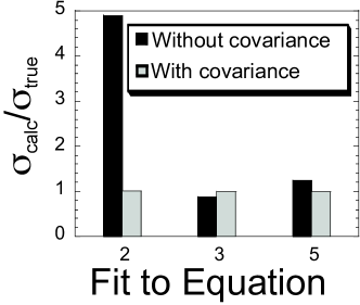
We therefore examined whether standard deviations calculated using only the first two terms were reasonable compared to using the full expression (Fig. 3). For example, we first fitted to Eq. 2 to obtain best fit values of $\Delta_{r}G_{0}$ and $m$ as well as the error estimates and covariance between these parameters. We then used Eq. 7 with either just the two first terms (variance alone) or all three (including covariance) to estimate the error of $D_{50}$. It is clear that the last term of the error-propagation equation cannot be ignored meaning that the covariance between the fitted parameters is large. Thus, while one can estimate errors on $\Delta_{r}G_{0}$ from those on $D_{50}$ and $m$ (Clarke and Fersht,, 1993), one cannot obtain accurate errors in $D_{50}$ from $\Delta_{r}G_{0}$ and $m$.

Figure 3: Parameter correlation makes it difficult to propagate errors. Standard deviations were calculated from the error propagation equation (Eq. 7) using either only the first two terms (black bars) or all three terms (grey bars), i.e. including the covariance. The height of the bar indicates the ratio between the calculated standard deviation and that obtained directly from nonlinear least squares regression. The results shown here were generated from the $m=4\ kJmol^{-1}M^{-1}$ and $D_{50}=3M$ dataset, but all gave similar results. Calculations were carried out using all three versions of the LEM, so that for Eq. 2 the derived parameter is $D_{50}$, for Eq. 3 it is $\Delta_{r}G_{0}$ and for Eq. 5 $m$ is the derived parameter. It is seen that for Eq. 2, it is essential to know the covariance in order to calculate the standard deviation of the last parameter. The other two versions do not suffer from this problem.

The above observations suggests that this particular parameterization of the LEM suffers from parameter correlation during the nonlinear least-squares regression. Parameter correlation is a mathematical feature indicating that the determination of one parameter by the nonlinear least-squares procedure is not independent of the determination of another. The reason is that an increase in the sum-of-squares target function when one parameter changes is partially compensated by a change in the correlated parameter. It is important to note that correlation of this kind has nothing to do with a physical correlation. To quantify the degree of correlation between parameters in the three different version of the LEM we calculated correlation coefficients (Eq. 6) for all nine dataset and using all three parameterizations. The average correlation coefficient between $\Delta_{r}G_{0}$ and $m$ in Eq. 2 is 0.99 with the lowest observed value being 0.98. This indicates a very high degree of correlation. The other two versions of the LEM do not suffer from the same problem. The average correlation between $m$ and $D_{50}$ in Eq. 3 is 0.1 with values ranging from -0.5 to 0.6. In Eq. 5 the average correlation coefficient between $\Delta_{r}G_{0}$ and $D_{50}$ is 0.2 (-0.4 to 0.7). For these reasons, error propagation using just the variance terms are almost the same as also including the covariance (Fig. 3).

The issue of parameter correlation was further studied by a Monte Carlo analysis (Fig. 4). We generated 500 sets of synthetic data and each was analysed by nonlinear least-squares using one of equations 2, 3 or 5. For each parameterisation of the LEM, we plot the value of the two parameters that resulted from these fits (Fig. 4). The results show very clearly that in the case of Eq. 2, the value obtained of one parameter is highly dependent of that of the other. Also, it is evident that equations 3 and 5 do not suffer as badly from this problem.

Figure 4: Parameter distributions estimated by a Monte Carlo analysis. We carried out 500 rounds of Monte Carlo simulation by generating noiseless data from the best-fit parameters and subsequently adding normally distributed noise. Each dataset was analysed by nonlinear least-squares and parameters estimated. This was repeated for all three parameterizations of the LEM and the figure shows the result by plotting each pair of parameters against each other. Note how the parameters obtained using Eq. 2 are highly correlated. The horizontal and vertical lines indicate 68% confidence intervals for each parameter as estimated by the marginal method.

The Monte Carlo analysis also highlights a specific issue with the notion of confidence intervals when parameters are highly correlated. The lines in the plots indicate 68% confidence intervals of each parameter as obtained from the marginal method (Fig. 4). In the case of Eqs. 3 and 5, the area covered jointly by the individual confidence intervals correspond quite accurately to the region found by the Monte Carlo analysis. On the other hand, for Eq. 2 it is clearly evidence that the knowledge of the individual confidence intervals of $\Delta_{r}G_{0}$ and $m$ is not sufficient to generate the joint confidence region for the two parameters. Rather, the confidence region spanned by the two individual confidence intervals (the inner square) grossly overestimates the area of the confidence region.This is one of the major reasons why correlated parameters should be avoided when possible (Williams and Hall,, 2000; Johnson,, 2000). The observation that the individual confidence intervals are insufficient to determine the joint confidence region is exactly the reason for why covariances are necessary to calculate the standard deviation of $D_{50}$ using the error-propagation equation (Fig. 3).

Plots like those in Fig. 4 may also be used to compare denaturation data either under different experimental conditions or for different mutants (Williams and Hall,, 2000). An example is shown in Fig. 5 where stability parameters for all nine synthetic dataset are plotted as scatter plots from a Monte Carlo analysis. The plots are two-dimensional projections of the three-dimensional parameter space spanned by $\Delta_{r}G_{0}$, $m$ and $D_{50}$ and give an alternative way of comparing the unfolding behaviour of e.g. a set of mutants. This type of plot gives an simple way of comparing both the value of the parameters and their confidence intervals, and may reveal differences that might otherwise not have been noticed.

Figure 5: Comparison of protein stability parameters using scatter plots. We carried out a Monte Carlo analysis for all nine synthetic datasets. Each pair of parameters are plotted against each other. The colour coding at the right shows the $m$ and $D_{50}$ values used to generate the original dataset.

Another way of illustrating the correlation between the parameters uses so-called profile traces (Bates and Watts,, 1988). These are obtained by fixing one of the parameters at some given value and estimating the others by nonlinear least-squares analysis. In the case of non-correlated parameters, the value of one parameter should not depend on that of the other. If this procedure is repeated at a number of values for the fixed parameter and the two parameters are then plotted against each other, one would then expect an approximately straight line, parallel to the axis of the fixed parameter. If this is repeated with the other parameter fixed and subsequently all data are plotted, the result would be two orthogonal lines each parallel to a parameter axis. In contrast, in the case of correlated parameters, the value of one parameter would be dependent of that of the other, and therefore the two curves would neither be independent nor parallel to either axis. In fact, the slope of the line is determined by the correlation coefficient for the two parameters and equal slopes for the two lines are obtained in the case of $corr(p_{1},p_{2})=\pm 1$.

We determined profile traces for the three versions of the LEM using one of the synthetic dataset (Fig. 6). Again, parameters obtained using Eq. 2 are seen to be correlated since the change of one parameter is accompanied by a change in the other. Therefore the two curves coincide. This is not the case for the other two equations. It should be noted that only in the case of a strictly linear model will the lines be straight and in fact it can be shown that the curvature of the lines is an estimate for the nonlinearity of the model (Bates and Watts,, 1988).

Figure 6: Profile traces (Bates and Watts,, 1988) of parameters in the linear extrapolation methods. The denaturation data were analysed by fixing one of the parameters in the LEM and estimating the other by nonlinear least-squares. This was repeated at several fixed values for both parameters. The results shown here are from one of the nine synthetic data set. Similar results were obtained from the other eight. Two independent lines, as observed for equations 3 and 5, show that the parameters in these equations are not very correlated. The curvature of the lines is related to the nonlinearity of the problem. In contrast, for Eq. 2 the two lines superimpose. This is a consequence of the correlation between $\Delta_{r}G_{0}$ and the $m$-value.

In addition to visualising the parameter coupling in Eq. 2, the profile traces are also relevant to analyses of experimental data in other way. In particular, because $m$ and $\Delta_{r}G_{0}$ are correlated, a common approach for estimating changes in stabilities between e.g. wild type and a mutant ($\Delta\Delta_{r}G_{0}$) uses a fixed (shared) $m$ value for both proteins and estimates $\Delta\Delta_{r}G_{0}\approx\langle m\rangle(D_{50}^{\textrm{mut}}-D_{50}^{\textrm{wt}})$ (Kellis Jr et al.,, 1989). The profile traces validates this approach by showing that the estimated value of $D_{50}$ is rather insensitive to any noise that might be present when fitting the $m$-value, so that as long as the assumption that the $m$ value is the same for wild type and mutant is valid, then this approach should indeed be highly accurate.

Analysing experimental data

The analyses described above used synthetic data to demonstrate substantial parameter correlation between $\Delta_{r}G_{0}$ and the $m$-value when these are obtained from fits to Eq. 2 . To examine the extent to which these issues also pertain to experimental data we repeated some of these analyses using previously measured denaturation data for the protein LTP1 at three different values of pH (pH 3.2, 5.1 and 8.5) (Lindorff-Larsen and Winther,, 2001). As with the synthetic data we find substantial correlations between the fitted parameters when Eq. 2 is used, but also sizeable correlations between $m$ and $D_{50}$ in Eq. 3 (Table 2).

Table 2: Correlation coefficient between parameters in the three versions of the linear extrapolation method.

Eq.	pH 3.2	pH 5.1	pH 8.5	Parameters
2	0.97	0.99	1.0	$\Delta_{r}G_{0},m$
3	-0.55	-0.52	-0.20	$m,D_{50}$
5	-0.34	-0.40	-0.11	$\Delta_{r}G_{0},D_{50}$

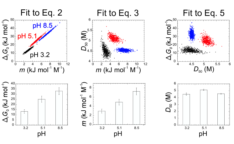
This correlation is also evident when repeating the analysis from the synthetic data (Fig. 5) using the data from LTP1 (Fig. 7). In line with the calculated correlation coefficients (Table 2) the plots show varying levels of correlations with strong correlations when fitting to Eq. 2, intermediate correlations from Eq. 3 and weak correlations from Eq. 5. In addition we note that analysing two-dimensional projections of the fitted parameters (Fig. 7, top) provides a clearer separation of the fitted parameters at the different values of pH, compared just just examining the individual fitted values (Fig. 7, bottom). Further, the higher value of $D_{50}$ at pH 5.1 (5.1 M) compared to the values at pH 3.2 and 8.5 (4.5 M and 4.6 M, respectively) manifests itself as a slight upward shift in the distribution of $\Delta_{r}G_{0}$ and $m$ when fitting to Eq. 2.

Figure 7: Comparison of protein stability parameters using scatter plots. Top row: Data are from LTP1 at pH 3.2 (black), 5.1 (red) and 8.5 (blue). Each pair of parameters in the LEM are compared. Parameters were generated by a Monte Carlo procedure as in Fig. 5. In the bottom row data are presented as bar diagrams for each parameter. The standard deviation of each parameter is shown as an error bar.

We also generated profile traces (Bates and Watts,, 1988) using the LTP1 data at pH 8.5 as an example (Fig. 8). Again, the strong correlation is evident when Eq. 2 is used so that when e.g. the $m$-value is fixed (and scanned in steps) the $\Delta_{r}G_{0}$ changes in full concert. In contrast, when Eq. 3 is used and the $m$-value is again scanned, the resulting $D_{50}$ value depends much less on the choice of $m$.

Figure 8: Profile traces (Bates and Watts,, 1988) of parameters fitted to the LTP1 denaturation data at pH 8.5. As for the synthetic data, two independent lines, as observed for equations 3 and 5, show that these parameters are not strongly correlated. The curvature of the lines is related to the non-linearity of the problem. In contrast, for Eq. 2 the two lines superimpose, which is a consequence of the correlation between $\Delta_{r}G_{0}$ and the $m$-value.

Discussion

A major goal in quantative analysis of experimental data is to obtain estimates of relevant parameters as well as estimates of what level of confidence in those parameters one should have. In the case of parameter estimation by nonlinear regression, many software packages estimate errors and confidence intervals use the variance-covariance matrix. Because that method is only strictly accurate for linear equations, it is not obvious whether that or some of the other methods for estimating fitting errors would be the best in the case of protein stability measurements. We therefore compared several different methods for obtaining confidence intervals using synthetic data with well defined statistical properties. Our results show that although the confidence interval estimates are similar, they may differ by a factor of two when obtained by different methods. We therefore evaluated the performance of four different methods using a large set of synthetic data. Our results show that the simplest method performs the best (Table 1). Further, this is even the case when non-normal experimental noise is simulated from a distribution function with wide tails. We therefore suggest that for most standard analyses, confidence intervals estimated by this method will suffice — a fortunate conclusion since this is also the method implemented in most software packages. In some cases it may, however, be appropriate to complement this estimate with a Monte Carlo estimate, in particular in the case of very noisy data.

We also examined the known problem of parameter correlation when the fitting protein stability data using Eq. 2 (Williams and Hall,, 2000). We note that similar issues have also been noted in the analysis of data from protein folding kinetics (Ruczinski et al.,, 2006). Our results show that the minimum of the sum-of-squares function when using Eq. 2 is long and narrow and is not aligned with the parameter axes. Several problems exist when fitting equations with correlated parameters. These include the problems of constructing joint confidence intervals and in the application of statistical tests. This is unfortunate since Eq. 2 uses $\Delta_{r}G_{0}$ and the $m$-value as parameters. These two parameters are those of the three that are generally of greatest interest because (i) the extrapolated value $\Delta_{r}G_{0}$ is generally assumed to be a good estimate of the unfolding free energy in the absence of denaturant and (ii) the $m$-value is known to correlate with changes in accessible surface area during unfolding (Myers et al.,, 1995; Geierhaas et al.,, 2007).

We, however, also show that two alternative parameterizations of the LEM, Eq. 3 and 5, suffer much less from parameter correlation, likely because they include $D_{50}$ which is the best determined of the parameters. Whereas a small change in $\Delta_{r}G_{0}$ may be compensated by one in $m$ in Eq. 2, this is not possible for the other equations since $D_{50}$ is determined much better by the experimental data. Similarly, if $D_{50}=\Delta_{r}G_{0}/m$ is the parameter best determined by the experiments, it is clear that $\Delta_{r}G_{0}$ and $m$ will be positively correlated. We show that due to parameter correlation, it is not possible to estimate confidence intervals for $D_{50}$ from the confidence intervals of $\Delta_{r}G_{0}$ and $m$, and suggest that it is safest also to specify $D_{50}$ explicitly.

Finally, our analyses support the use of a variant of Eq. 3 to estimate changes in stability between two protein variants. Our profile trace analysis show that $D_{50}$ can be robustly determined even if the $m$ value is not accurate, supporting the common practice of combining an estimate of the mean $m$ value and changes in $D_{50}$ to estimate changes in protein stability.

References

- Amsdr et al., (2019) Amsdr, A., Noudeh, N. D., Liu, L., and Chalikian, T. V. (2019). On urea and temperature dependences of m-values. The Journal of chemical physics, 150(21):215103.
- Bard, (1974) Bard, Y. (1974). Nonlinear parameter estimation. Academic press.
- Bates and Watts, (1988) Bates, D. M. and Watts, D. G. (1988). Nonlinear regression analysis and its applications, volume 2. Wiley New York.
- Bevington et al., (1993) Bevington, P. R., Robinson, D. K., Blair, J. M., Mallinckrodt, A. J., and McKay, S. (1993). Data reduction and error analysis for the physical sciences. Computers in Physics, 7(4):415–416.
- Box, (1960) Box, G. E. (1960). Fitting empirical data. Annals of the New York Academy of Sciences, 86(3):792–816.
- Box and Muller, (1958) Box, G. E. and Muller, M. E. (1958). A note on the generation of random normal deviates. Ann. Math. Stat., 29:610–611.
- Brandts, (1969) Brandts, J. F. (1969). Conformational transitions of proteins in water and in aqueous mixtures. Structure and stability of biological macromolecules, 2:213.
- Chernick, (1999) Chernick, M. R. (1999). Bootstrap methods: A guide for practitioners and researchers, volume 353. John Wiley & Sons.
- Clarke and Fersht, (1993) Clarke, J. and Fersht, A. R. (1993). Engineered disulfide bonds as probes of the folding pathway of barnase: increasing the stability of proteins against the rate of denaturation. Biochemistry, 32(16):4322–4329.
- Geierhaas et al., (2007) Geierhaas, C. D., Nickson, A. A., Lindorff-Larsen, K., Clarke, J., and Vendruscolo, M. (2007). Bppred: A web-based computational tool for predicting biophysical parameters of proteins. Protein Science, 16(1):125–134.
- Greene and Pace, (1974) Greene, R. F. and Pace, C. N. (1974). Urea and guanidine hydrochloride denaturation of ribonuclease, lysozyme, -chymotrypsin, and -lactoglobulin. Journal of Biological Chemistry, 249(17):5388–5393.
- Johnson, (2000) Johnson, M. L. (2000). Parameter correlations while curve fitting. In Methods in enzymology, volume 321, pages 424–446. Elsevier.
- Johnson et al., (1981) Johnson, M. L., Correia, J. J., Yphantis, D. A., and HalvorSON, H. R. (1981). Analysis of data from the analytical ultracentrifuge by nonlinear least-squares techniques. Biophysical journal, 36(3):575–588.
- Johnson and Faunt, (1992) Johnson, M. L. and Faunt, L. M. (1992). [1] parameter estimation by least-squares methods. In Methods in enzymology, volume 210, pages 1–37. Elsevier.
- Kellis Jr et al., (1989) Kellis Jr, J. T., Nyberg, K., and Fersht, A. R. (1989). Energetics of complementary side chain packing in a protein hydrophobic core. Biochemistry, 28(11):4914–4922.
- Knuth, (2014) Knuth, D. E. (2014). Art of computer programming, volume 2: Seminumerical algorithms. Addison-Wesley Professional.
- Lindorff-Larsen and Winther, (2001) Lindorff-Larsen, K. and Winther, J. R. (2001). Surprisingly high stability of barley lipid transfer protein, ltp1, towards denaturant, heat and proteases. FEBS letters, 488(3):145–148.
- Marquardt, (1963) Marquardt, D. W. (1963). An algorithm for least-squares estimation of nonlinear parameters. Journal of the society for Industrial and Applied Mathematics, 11(2):431–441.
- Matsumoto and Nishimura, (1998) Matsumoto, M. and Nishimura, T. (1998). Mersenne twister: a 623-dimensionally equidistributed uniform pseudo-random number generator. ACM Transactions on Modeling and Computer Simulation (TOMACS), 8(1):3–30.
- Moosa et al., (2018) Moosa, M. M., Goodman, A. Z., Ferreon, J. C., Lee, C. W., Ferreon, A. C. M., and Deniz, A. A. (2018). Denaturant-specific effects on the structural energetics of a protein-denatured ensemble. European Biophysics Journal, 47(1):89–94.
- Myers et al., (1995) Myers, J. K., Nick Pace, C., and Martin Scholtz, J. (1995). Denaturant m values and heat capacity changes: relation to changes in accessible surface areas of protein unfolding. Protein Science, 4(10):2138–2148.
- Pace and Shaw, (2000) Pace, C. N. and Shaw, K. L. (2000). Linear extrapolation method of analyzing solvent denaturation curves. Proteins: Structure, Function, and Bioinformatics, 41(S4):1–7.
- Ruczinski et al., (2006) Ruczinski, I., Sosnick, T. R., and Plaxco, K. W. (2006). Methods for the accurate estimation of confidence intervals on protein folding -values. Protein science, 15(10):2257–2264.
- Santoro and Bolen, (1988) Santoro, M. M. and Bolen, D. (1988). Unfolding free energy changes determined by the linear extrapolation method. 1. unfolding of phenylmethanesulfonyl. alpha.-chymotrypsin using different denaturants. Biochemistry, 27(21):8063–8068.
- Schellman, (1994) Schellman, J. A. (1994). The thermodynamics of solvent exchange. Biopolymers: Original Research on Biomolecules, 34(8):1015–1026.
- Schellman, (2002) Schellman, J. A. (2002). Fifty years of solvent denaturation. Biophysical chemistry, 96(2-3):91–101.
- Seber and Wild, (1989) Seber, G. and Wild, C. (1989). Nonlinear regression john wiley & sons. New York.
- Straume and Johnson, (1992) Straume, M. and Johnson, M. L. (1992). [7] monte carlo method for determining complete confidence probability distributions of estimated model parameters. In Methods in enzymology, volume 210, pages 117–129. Elsevier.
- Tanford, (1970) Tanford, C. (1970). Protein denaturation. Adv. Protein Chem, 24(1):95.
- Williams and Hall, (2000) Williams, D. J. and Hall, K. B. (2000). Monte carlo applications to thermal and chemical denaturation experiments of nucleic acids and proteins. In Methods in enzymology, volume 321, pages 330–352. Elsevier.
- Yi et al., (1997) Yi, Q., Scalley, M. L., Simons, K. T., Gladwin, S. T., and Baker, D. (1997). Characterization of the free energy spectrum of peptostreptococcal protein l. Folding and Design, 2(5):271–280.