Stripped-envelope core-collapse supernova ⁵⁶Ni masses:

Abstract

Context. The mass of synthesised radioactive material is an important power source for all supernova (SN) types. Anderson (2019) recently compiled literature values and obtained ${}^{56}\mathrm{Ni}$ distributions for different core-collapse supernovae (CC SNe), showing that the ${}^{56}\mathrm{Ni}$ distribution of stripped envelope CC SNe (SE-SNe: types IIb, Ib, and Ic) is highly incompatible with that of hydrogen rich type II SNe (SNe II). This motivates questions on differences in progenitors, explosion mechanisms, and ⁵⁶Ni estimation methods.

Aims. Here, we re-estimate the nucleosynthetic yields of ${}^{56}\mathrm{Ni}$ for a well-observed and well-defined sample of SE-SNe in a uniform manner. This allows us to investigate whether the observed SN II–SE SN ${}^{56}\mathrm{Ni}$ separation is due to real differences between these SN types, or because of systematic errors in the estimation methods.

Methods. We compiled a sample of well observed SE-SNe and measured ${}^{56}\mathrm{Ni}$ masses through three different methods proposed in the literature. First, the classic ‘Arnett rule’, second the more recent prescription of Khatami & Kasen, and third using the tail luminostiy to provide lower limit ${}^{56}\mathrm{Ni}$ masses. These SE-SN distributions were then compared to those compiled by Anderson.

Results. Arnett’s rule - as previously shown - gives ${}^{56}\mathrm{Ni}$ masses for SE-SNe that are considerably higher than SNe II. While for the distributions calculated using both the Khatami & Kasen prescription and Tail ${}^{56}\mathrm{Ni}$ masses are offset to lower values than ‘Arnett values’, their ${}^{56}\mathrm{Ni}$ distributions are still statistically higher than that of SNe II. Our results are strongly driven by a lack of SE-SN with low ${}^{56}\mathrm{Ni}$ masses (that are in addition strictly lower limits). The lowest SE-SN ⁵⁶Ni mass in our sample is of 0.015${\rm\ M}_{\odot}$, below which are more than 25% of SNe II.

Conclusions. We conclude that there exists real, intrinsic differences in the mass of synthesised radioactive material between SNe II and SE-SNe (types IIb, Ib, and Ic). Any proposed current or future CC SN progenitor scenario and explosion mechanism must be able to explain why and how such differences arise, or outline a yet to be fully explored bias in current SN samples.

1 Introduction

One of the big unresolved questions in SN science is the connection of different types of stellar explosions with possible stellar progenitors. In the case of CC SNe, that arise from the collapse of the iron core of massive stars, a way to probe the progenitor core structure and the explosion mechanism is to study the nucleosynthesis yields of the explosion. In particular the radioactive yield of ⁵⁶Ni is a useful probe of the explosion physics (e.g. Suwa et al. 2019 and references therein) and it is a fundamental parameter driving the evolution of SN light emission in the first few hundred days (e.g. Colgate & McKee 1969).
CC SNe can be broadly separated into those that show long, persistent hydrogen features in their spectra (hydrogen-rich SNe II) and those that do not (see Gal-Yam 2017 for a recent review of SN observational classifications). The latter are broadly classed as ‘stripped envelope’ events (SE-SNe, as above) where the nomenclature refers to the progenitor exploding without most of its outer hydrogen (types IIb and Ib) or additionally helium (Ic) envelopes retained at the epoch of explosion. An analysis into the mass of ⁵⁶Ni sythesised in the explosion of SE-SNe is the focus of this paper.
When a successful CC SN explosion occurs, a shock wave propagates outwards and produces explosive nucleosynthesis in the inner parts of the ejecta (composed mainly of silicon and oxygen) that for a short period of time acquires high temperatures of $\sim 5\cdot 10^{9}$ K (required to produce the radioactive yields of ⁵⁶Ni). The shock soon sweeps through the entire ejecta, homologous expansion is achieved and the highly ionized ejecta cools in very close to adiabatic conditions. The early light curve for a hydrogen deficient SE-SN consists of a very fast decline-cooling stage where the thermal emission of the ejecta is highly reduced by the temperature decrease due to expansion cooling. At the same time the ionization of the ejecta is reduced and recombination settles in which may give rise to a short plateau of a few days (e.g. Ensman & Woosley 1988; Dessart et al. 2011). After this stage the input from radioactive decay, in the form of gamma rays and positrons, becomes fundamental as the heat wave it produces in the inner layers finally encounters the receding photosphere of recombining material, which gives rise to stabilization or increase in the photospheric temperature and the light curve starts to rise to peak. The following light curve behaviour depends on the amount and spatial distribution of the heating material with respect to the bulk of the ejecta. In general the light curve will rise to a peak luminosity that increases with the amount of heating material and will decline in a time scale that depends on the photon diffusion time scale, which grows with the ejecta opacity and mass. Additionally, the amount of mixing of the heating source also effects the timescales in that for larger mixing (i.e. the radioactive material is found out to a larger radius) the heat wave reaches the outer envelope faster and the gamma ray escape probability will be higher for the ejecta. After peak luminosity, the light curve slope will smoothly approach the slope of the radioactive heating decay, modulo the decreasing deposition function of gamma rays, as it approaches the optically thin regime (Dessart et al., 2016). This simple scenario and physical assumptions is the basis for the measurement of ⁵⁶Ni masses from observations.
Recently, Anderson (2019) compiled a large sample of literature ⁵⁶Ni measurements for CC SNe and found significant differences between the ⁵⁶Ni distributions of SNe II and SE-SNe estimated by the community. Anderson argued that such large differences in ⁵⁶Ni masses were inconsistent with currently favoured progenitor and explosion models of CC SNe where significant differences are not expected between the different types. That work compiled many different estimations from many different authors in the literature and therefore combined a large number of different methodologies. Here, our aim is to investigate whether these recent results are due to errors in the ⁵⁶Ni estimation methods, or whether true intrinsic ⁵⁶Ni differences do exist between SNe II and SE-SNe. We do this by concentrating our efforts on ⁵⁶Ni estimation in SE-SNe, through compiling a well-defined and well-observed sample of literature SE-SN photometry, and re-estimating ⁵⁶Ni masses. These masses are estimated using different formalisms from the literature and are then once again compared to the ⁵⁶Ni distribution of SNe II. We find that the ⁵⁶Ni mass difference persists between SE-SNe and SNe II.
The paper is organised as follows. In the next section we describe our data sample selection. Then in Section 3 we outline how we produce our pseudo-bolometric light curves and the methods used to extract ⁵⁶Ni masses from them. Section 4 presents our new SE-SN ⁵⁶Ni mass distributions and compares them to SNe II, then the implications of these findings are further discussed in Section 5. Finally, we present our main conclusions in Section 6.

2 Data and sample selection

To collect the most complete SE-SN sample possible we searched for photometric data listed on the open supernova catalog (Guillochon et al., 2017). Besides using publications of individual SNe, we used samples from the Harvard-Smithsonian Center for Astrophysics (CfA) (Bianco et al., 2014), the Carnegie Supernova Project (CSP-I) (Taddia et al., 2018), and the Sloan Digital Sky Survey (SDSS) SN survey II (Taddia et al., 2015). The wavelength coverage and cadence of the photometric observations is highly varied, from just a couple of optical-wavelength observations at a few epochs, to a wide coverage from the NUV to the NIR and with several observations from close to explosion out to nebular phases, more than 100 days post peak luminosity. This full compilation comprises 133 SE-SNe. From this initial sample, we selected SE-SNe with coverage in the optical $BVRI$ (or SDSS analogues $gri$) and near-infrared (NIR) $YJH$ bands. Then, objects are also removed that do not have photometry covering phases close to the peak. SE-SNe are retained if they have at least one data point before and after the estimated peak luminosity in the bolometric light curve (see below our procedure to obtain the bolometric light curves). For an individual SN, if there was more than one source of photometry in a given band, we checked whether they were consistent. If they were significantly different considering the errors, and if it was not possible to determine the reason (e.g. different zero-points or photometric systems) the discrepant source with less data was simply removed. Following the above selection criteria we obtain a sample of 37 SE-SNe (listed in Table 2).

3 Methods

Here we first outline how we produce bolometric light curves for our sample and then summarise the different methods used to estimate ⁵⁶Ni masses.

3.1 Bolometric light curves

After compiling the photometry, the steps used to obtain bolometric light curves for each SN were as follows:

• We first selected the time window $(t_{min},t_{max})$ within which the SN has photometry in those bands within the $B$ to $H$ range. This conservative interval was chosen so as to avoid data extrapolation. Only in the extreme case that a photometric band barely covered the peak, did we linearly extrapolate the data up to a maximum of 7 days, including an extrapolation error of 0.5 magnitudes. If there was a band that limited too much the final time range of the bolometric light curve, the band was removed: except for the case of $B$ or $H$ photometry where their removal would shorten the wavelength range.

• Given the time window from above, we chose to interpolate all photometry to the epochs of the filter having the most homogeneous coverage. To define this filter, we used the entropy measure of the coverage distribution (i.e. the histogram/distribution of the epochs observed, ${p_{k}}$) of each filter, which is calculated by the Shannon formula,

  $$S=-\sum_{k}p_{k}\cdot log(p_{k})$$ (1)

  and the filter with the maximum entropy value was chosen. We then linearly interpolated all the other bands to the epochs of the filter as defined above, providing us with magnitudes evaluated in the same baseline $m(\{t_{i}\})$.

• Before converting to flux we corrected the magnitudes for the Galactic reddening (Schlafly & Finkbeiner, 2011) using a standard Cardelli extinction law with $R_{V}=3.1$. Although probably uncertain (see later discussion), we also corrected for host galaxy extinction using values from the relevant references (see Table 2).

• All photometry was transformed to the AB system and flux densities were calculated using standard formulae. An example resulting spectral energy distribution (SED) is shown in Figure 1.

• Fluxes $F_{\nu}(t_{i})$ were integrated in frequency space using Simpson’s rule. With this integrated flux $F(t_{i})$ the luminosity was then obtained using the luminosity distance,

  $$L(t_{i})=4\pi d_{L}^{2}F(t_{i})$$ (2)

  and we do not extrapolate the fluxes outside our defined wavelength range of $B$ to $H$. Therefore, our resulting light curves should be considered pseudo-bolometric, and are a lower limit to the true bolometric luminosity at all times.

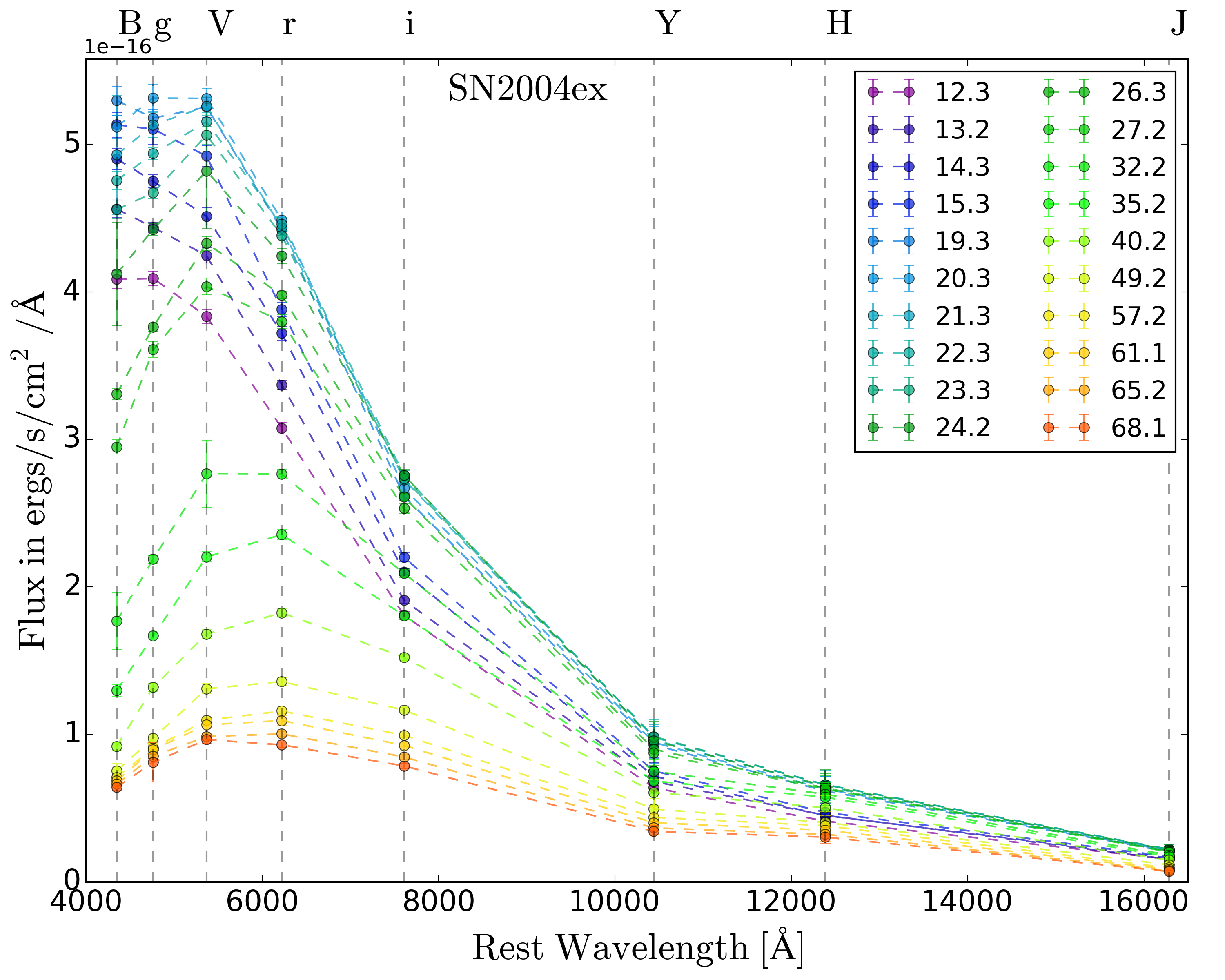
Figure 1: Example of the temporal SED evolution for the type IIb SN 2004ex. Each SED is colour coded by the time since explosion (listed in the legend, in days). Each filter is labeled with a dashed vertical line and the name of the filter is given on the top axis.

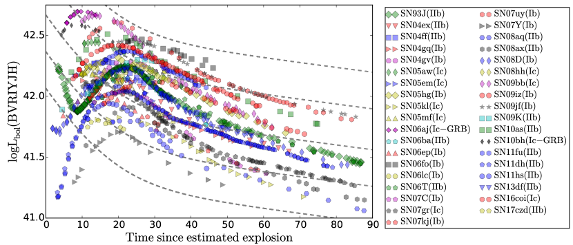
Figure 2: $BVRIYJH$ bolometric light curves for our sample of 37 SE-SNe. SN types are listed in the legend. The dashed grey curves show reference ⁵⁶Ni decays, with a factor of two in ⁵⁶Ni mass separation. From these reference slopes its can be seen that all SE-SNe within our sample decline steeper than the ⁵⁶Ni decay after $\sim 60$ days past explosion.

Our $BVRIYJH$ bolometric light curves for the full sample are presented in Fig. 2. This sample has a total 14 SNe IIb, 13 SNe Ib, 6 normal SNe Ic, 2 SNe Ic-BL and 2 SNe Ic-GRB. While the calculated values for these two SNe Ic-GRB are presented in this paper, they are not included in the comparison to the SN II population. This is because these objects show the largest degree of asphericities among SE-SN (Maeda et al., 2008), and their emission may also have a significant contribution from sources other than radioactive decay (e.g. Wang et al., 2017; Lü et al., 2018). To obtain peak luminosities we applied a local polynomial regression with a Gaussian kernel, using the public modules from PyQt-fit in Python. The smoothing function obtained is sampled in a dense grid and the maximum is obtained directly from this grid. Using explosion epochs as estimated in literature references (see Table 2), we obtained the rise time ($t_{rise}$ or $t_{peak}$) distributions that are presented and discussed in Appendix A.

3.2 Methods to measure ⁵⁶Ni masses

We now outline the three methods used to estimate ⁵⁶Ni masses for our SE-SN sample. To date, the most commonly used method in the literature is the application of the so called “Arnett rule” (Arnett, 1982). This “rule” is derived analytically from a simple model with several assumptions (see Khatami & Kasen 2019 for a discussion of the assumptions involved). The rule states that the luminosity at peak, $L_{peak}$ is equal to the instantaneous power from radioactive decay $L_{heat}$, which for the case of ⁵⁶Ni decay can be written as,

$$L_{peak}=L_{heat}(t_{peak})=\frac{M_{Ni}}{M_{\odot}}\left[(\epsilon_{Ni}-\epsilon_{Co})e^{-t_{peak}/t_{Ni}}+\epsilon_{Co}e^{-t_{peak}/t_{Co}}\right]$$ (3)

where $\epsilon_{Ni}=3.9\cdot 10^{10}$ erg/s/g, $\epsilon_{Co}=6.78\cdot 10^{9}$ erg/s/g, $t_{Ni}=8.8$ days and $t_{Co}=111.3$ days (with ⁵⁶Co being the daughter product of ⁵⁶Ni).

The other established method to estimate ⁵⁶Ni masses uses the bolometric luminosity at nebular phases, when the ejecta is optically thin. In this phase gamma rays are expected to be fully or partially trapped in the ejecta and the reprocessed energy is released entirely. With the assumption that the gamma rays are fully trapped in the ejecta the bolometric light curve should follow equation 3 and obtaining the ⁵⁶Ni mass is trivial, measuring the bolometric luminosity at a given epoch in the radioactive tail. However, this formalism has generally not been applied to SE-SNe in the literature, while it is the standard method to estimate SN II ⁵⁶Ni masses. In the case of SNe II, light-curve tail decline rates generally follow that predicted by ⁵⁶Co decay (see e.g. Anderson et al. 2014). However, this is not the case for SE-SNe (as can be seen in Fig. 2). Still, even though SE-SN light curves decline quicker than the predicted rate, the Tail can be used to estimate a lower limit for the ⁵⁶Ni mass, and that is what we do here. To ensure that we use luminosities when the light curve has entered the nebular phase, we selected epochs in the bolometric light curve that fulfilled the condition:

$$t>\min(t_{peak}+2t_{half},t_{peak}+25)$$ (4)

where $t_{half}$ is the time taken for the light curve to decline from peak luminosity to half that value. The last three of these epochs were then fitted with the relation in equation (3) giving our lower limit ⁵⁶Ni mass.

Recently, a new method was proposed to measure (amongst other things) the ⁵⁶Ni masses in SNe (Khatami & Kasen, 2019). Here, ⁵⁶Ni masses are derived through an integration of the equation for the global energy conservation, using several assumptions on the temporal behaviour of the heating source and internal energy. The Khatami & Kasen formalism gives rise to the simple relation:

$$L_{peak}=\frac{2}{\beta^{2}t_{peak}^{2}}\int_{0}^{\beta t_{peak}}{tL_{heat}(t)dt}$$ (5)

$\beta$ parameterises the degree of mixing and changing opacity in the ejecta. To calculate ⁵⁶Ni masses for our SE-SN sample using this relation we use the suggested values of $\beta$ in Khatami & Kasen (2019), from their Table 2: 0.82 for SNe IIb, and $9/8$ for SNe Ib and SNe Ic (including SNe Ic-BL). We note here that there does not appear to be strong evidence for the use of these specific $\beta$ values. Indeed, assuming one $\beta$ value for SE-SNe of different ejecta mass may be too simplistic.
When possible, ⁵⁶Ni masses are derived for all SE-SNe in our sample through the three procedures outlined above. Fig. 3 shows an example well-sampled bolometric light curve (SN 2004ex) with the ⁵⁶Ni decay curves plotted derived from the synthesised ⁵⁶Ni mass from each procedure. The distributions resulting from all SE-SNe used in this work are now discussed in detail.

Figure 3: Example light curve and analysis results for the well sampled $BVRIYJH$ bolometric light curve of SN 2004ex. The dashed-dotted, dashed, and dotted lines marks the ⁵⁶Ni decay, assuming an initial ⁵⁶Ni mass given by Arnett’s rule, the Khatami & Kasen (2019) method (dubbed “k&k”), and the lower limit from the Tail respectively. The fit used to obtain the maximum of the light curve is shown as a green dashed line.

4 Results

Armed with the ⁵⁶Ni masses calculated in the previous section, we now compare the SE-SN distributions derived from the different methods and contrast these with the SN II distribution from Anderson (2019). In Fig. 4 we show cumulative distributions for the ⁵⁶Ni masses analysed in this work, where we combine all SE-SN types (IIb, Ib and Ic - but not Ic-BL). It is clear that the ⁵⁶Ni masses obtained using the Khatami & Kasen and Tail methods are significantly lower than those estimated through Arnett’s rule. However, Fig. 4 also shows that the SE-SN ⁵⁶Ni mass distributions from the first two methods still appear to be shifted towards higher values than that of the SN II. It is also clear from Fig. 4 that there are many SN II ⁵⁶Ni masses below the lowest SE-SN value (through all estimation methods). This point is discussed further in the next section.
In Table 1 the results of a two sample Kolmogorov-Smirnov (KS) and Anderson-Darling (AD) tests between the distribution of ⁵⁶Ni masses of SNe II and SE-SNe are presented. The result from Anderson (2019) is recovered here - for a smaller sample of SE-SNe, but using Arnett’s rule - in that SE-SNe present significantly higher ⁵⁶Ni masses than SNe II. While for the Tail and Khatami & Kasen methods the significance of this difference is reduced, the difference still persists: SE SNe in our sample produce more ⁵⁶Ni in their explosions than SNe II. We reiterate here: the Tail ⁵⁶Ni masses are lower limits given that for the majority of SE-SNe their tail luminosities decline more quickly than the rate predicted by ⁵⁶Co decay (Fig. 2) implying significant escape of the radioactive emission. We also note that Fig. 4 suggests that the ⁵⁶Ni masses derived from the Khatami & Kasen method and those from the Tail are more or less the same. Given that the latter are lower limits this implies that the former are probably underestimated, suggesting that our employed $\beta$ values are possibly in error (see additional discussion below). We do not attempt to evaluate differences between different SE-SN sub types here, given the low number of objects in each class.
Figure 5 presents a comparison of the ⁵⁶Ni masses derived through Arnett’s rule and the Khatami & Kasen method. The largest difference between the methods is for the SNe IIb, in that Arnett’s rule gives ⁵⁶Ni masses that are around twice as large as those of Khatami & Kasen. In the case of SN types Ib, Ic and Ic-BL Arnett generally gives values that are 25-50% higher than Khatami & Kasen. Finally, for our sample of well-observed SE-SNe presented here there are no ⁵⁶Ni masses larger than $\sim 0.2$ $M_{\odot}$ (0.21$M_{\odot}$ for the type Ib SN2007uy, using Arnett’s rule). Anderson (2019) discussed the existence of a tail of ⁵⁶Ni masses for SE-SNe out to extremely high values nearing 1${\rm\ M}_{\odot}$. The lack of such high values in the current SE-SN sample (that is well sampled in both wavelength and time) suggests that maybe those extreme literature values are in error due to a lack of observational data and/or errors in corrections such as those for host galaxy extinction. Alternatively, it is possible that those SE-SNe with high ⁵⁶Ni masses arise from distinct explosion mechanisms where radioactive decay is not the dominant luminosity source (see later discussion).
Before discussing the implications of our findings, in the next subsections we discuss possible systematics in ⁵⁶Ni mass estimations and how these may affect our results.

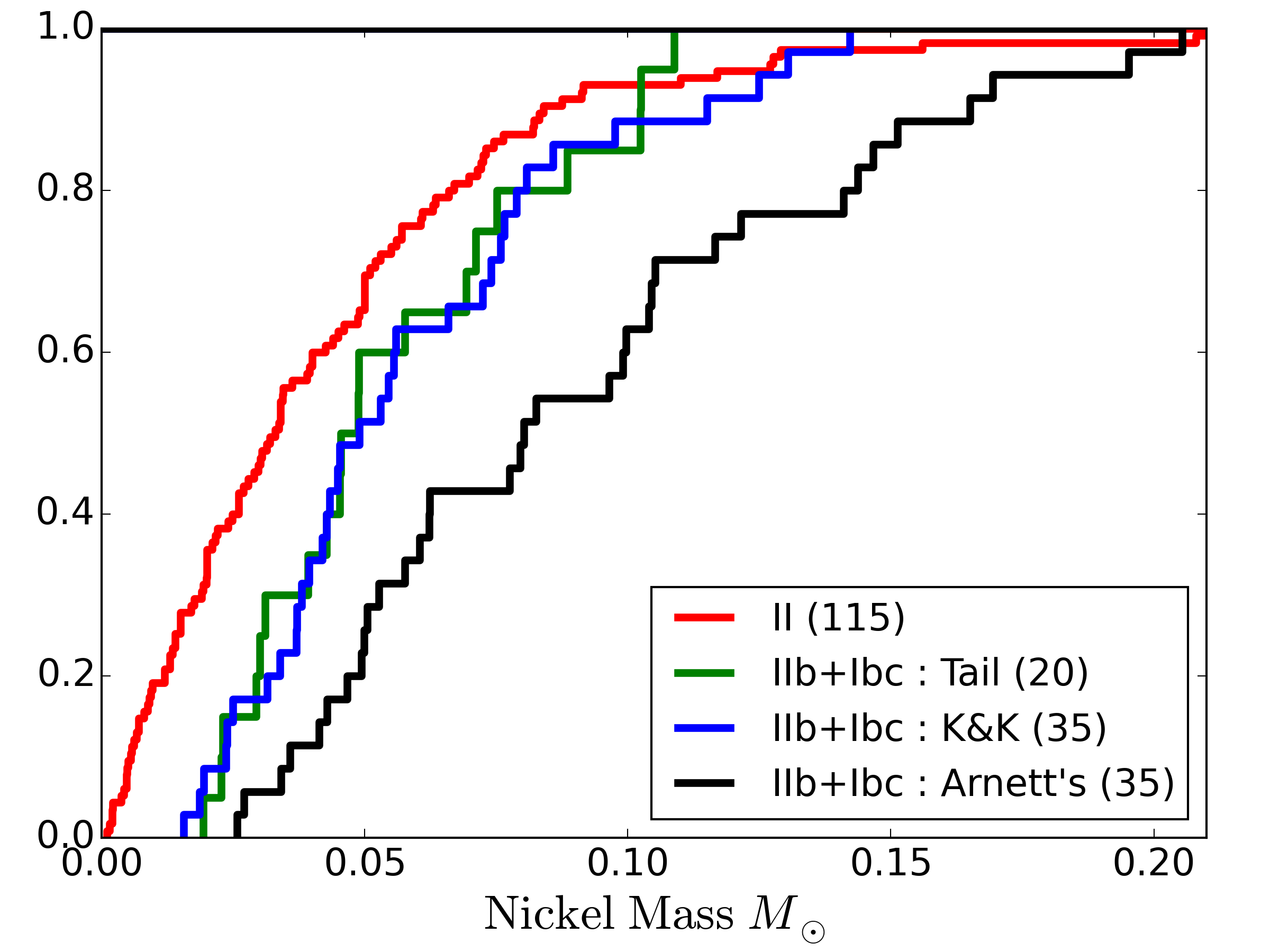
Figure 4: Cumulative distributions of SE-SN ⁵⁶Ni masses derived through the three methods outlined in the text compared to that of SNe II (Anderson, 2019).

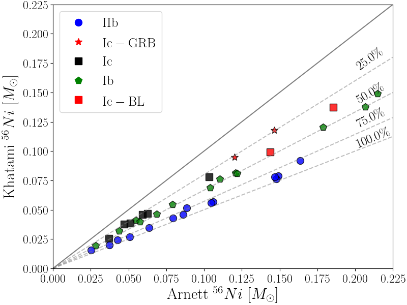
Figure 5: Comparison of the ⁵⁶Ni masses as measured by Arnett’s rule and the Khatami & Kasen prescription. The solid diagonal line shows the one to one relation between the two methods and the dashed lines show different percentual differences between them.

Table 1: Two sample KS and AD (two sided) tests between the distribution of ⁵⁶Ni masses of SNII (115 SNe) and SE-SNe (35 for Arnett, 35 for Khatami & Kasen, and 20 using the Tail).

	Kolmogorov-Smirnov test		Anderson-Darling test
Method	p-value	D	p-value	A
Tail	0.039	0.334	0.031	2.529
Khatami & Kasen	0.002	0.351	0.001	7.197
Arnett	6.694E-07	0.506	$<$1.000E-03	20.017

4.1 Systematics

While each ⁵⁶Ni mass estimation method described in Section 3.2 has its own caveats, all three are susceptible to uncertainties in (1) the explosion epoch $t_{0}$, (2) the bolometric correction used to extrapolate the missing flux, and (3) the employed host galaxy reddening values. Here, as outlined above, we do not use any bolometric correction. However, we only include SE-SNe in our sample that have data between $B$ and $H$ bands, and this selection criteria is applied consistently across the sample. While this removes the uncertainty of calculating bolometric luminosities from only a few optical photometric points (as has been done in previous works), it means that our estimated luminosities are ‘pseudo-bolometric’ and are lower limits to the true luminosity at any epoch. These pseudo-bolometric luminosities therefore translate to lower limits to estimated ⁵⁶Ni masses. However, this is not a problem for the main aim of this work. This work aims at testing whether there exist true differences in ⁵⁶Ni masses between SE-SNe and SNe II and in the previous subsection we conclude that indeed true, intrinsic differences persist in that SE-SNe produce more radioactive material than SNe II. Thus, our decision to not correct for the missing flux outside the $B$ and $H$ bands only reinforces our result: making full bolometric corrections would produce higher SE-SN ⁵⁶Ni masses and therefore produce even more statistically significant ⁵⁶Ni mass differences than we present.

4.1.1 Explosion epochs

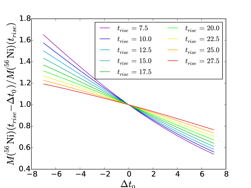
Figure 6: Fractional variation of the ⁵⁶Ni mass using the Arnett rule, as a function of the rise time variation in days. The shorter the real rise time the more the ⁵⁶Ni mass is affected by the unknown explosion epoch.

The effect of the uncertainty on the explosion epoch can be more easily tested. In Fig. 6 we show the fractional difference in the ⁵⁶Ni mass, changing the explosion epoch and using Arnett’s rule, for different intrinsic rise times. ⁵⁶Ni masses are increased with longer rise times. When changing the rise time $\pm 7$ days, the ⁵⁶Ni mass variation goes from $\pm 20\%$ for longer rise times of $\sim 20$ days, typical for a SN IIb, to $\pm 60\%$ for very short rise times of $\sim 10$ days, similar to SNe Ic.
Following the above, we test the dependence of our results on the uncertainty of our employed explosion epochs using the most extreme scenario possible: we redefine explosion epochs to be just one day before the discovery epoch. This effectively reduces the rise time to it’s minimal value and therefore pushes the ⁵⁶Ni mass to it’s minimal value (through this systematic). Re-calculating ⁵⁶Ni masses using these extreme explosion epochs, and again running a KS test on the SE-SN and SN II distributions, we find p-values of $\sim$10% for Khatami & Kasen, while the Tail and Arnett give 5% and 0.5%, respectively. Thus, while the statistical significance of differences in ⁵⁶Ni mass between the SN types is lessened (as of course expected), the difference still persists.
We emphasize that our extreme approach considers the very unlikely possibility that the discovery epochs are within a day of SN explosion. Therefore, we conclude that our results and conclusions are robust to explosion epoch uncertainties.

4.1.2 ⁵⁶Ni mixing

The Khatami & Kasen (2019) ⁵⁶Ni mass estimation method employs ‘$\beta$’ that paramterises the amount of ⁵⁶Ni mixing in the ejecta, which has a strong influence on the resulting ⁵⁶Ni mass. In Fig. 7 we show the fractional ⁵⁶Ni mass variation as a function of $\beta$ for SNe within different rise times. Suggested values for typical progenitor structures and composition are also shown. For rise times greater than 10 days, ⁵⁶Ni masses increase by up to a factor two higher when changing $\beta$ from $\sim$0.6 to $\sim$2.0. As $\beta$ appears only in the form $\beta t_{peak}$, changing $\beta$ is equivalent to changing the rise time. As was shown in Khatami & Kasen an increase in $\beta$ mimics an increase of ⁵⁶Ni mixing out through the SN ejecta. Arnett’s rule has been shown to be more valid for well mixed sources, corresponding to $\beta$ $\sim$1.9. Therefore, following the suggested values of $\beta$, Arnett’s rule is more accurate for ⁵⁶Ni mass estimations for SNe Ic than for SNe IIb (see Appendix A).
We now investigate how much Khatami & Kasen ⁵⁶Ni masses change when different $\beta$ values are assumed. As we want to test the robustness of our conclusion of distinct ⁵⁶Ni masses between SE-SNe and SNe II, we recalculate ⁵⁶Ni masses using the lowest value of $\beta=0.82$ for all the SE SN of our sample; i.e., that which will produce the lowest ⁵⁶Ni masses for SE-SNe. This new ⁵⁶Ni mass distribution - assuming $\beta=0.82$ - is then compared to that of SNe II and a KS test p-value of $3.4\%$ is obtained. Therefore, while the significance of the difference in the distributions is lessened (as one would expect), the difference is still present. In addition, assuming this low $\beta=0.82$ value produces many ⁵⁶Ni masses for SE-SNe lower than the Tail method. This does not make sense, as the ⁵⁶Ni masses from the tail luminosities are strict lower limits due to the non-negligible gamma ray escape fraction (see the steepness of light curve tails in Fig. 2). At the same time, this result suggests that for at least some SE-SNe ⁵⁶Ni is significantly mixed through the ejecta. Indeed, even using the suggested $\beta$ values, ⁵⁶Ni masses from Khatami & Kasen are more or less the same as those from the Tail. This latter observation suggests that ⁵⁶Ni may be even more mixed than implied by the suggested $\beta$ values. Future work should explore ways to estimate the ⁵⁶Ni mixing from observations (e.g. Yoon et al., 2019), in order to constrain $\beta$ and provide more accurate measurements.

4.1.3 Extinction

In Fig. 8 we show again the ⁵⁶Ni mass cumulative distributions (compared to that of SNe II), but this time we only correct SE-SN photometry for Galactic reddening, and neglect host galaxy extinction corrections. We do this to test the how much the uncertainty of host galaxy reddening corrections affects our results.
As expected, the cumulative distributions are now closer, with ⁵⁶Ni differences reduced. When repeating the KS tests we find that the difference between the Tail SE-SN and SN II (that have been corrected for host galaxy extinction) distributions is no longer statistically significant (p value of $28.6\%$). Statistically significant differences persist when using SE-SN values from Khatami ($0.022\%$) and Arnett ($<10^{-3}$ %). Thus, there is some suggestion that uncertainties in host galaxy extinction affect our results, and could explain some of the SE-SN–SNe II differences. However, the test here (as in the previous two subsections) is the extreme case that is very unlikely to be true. Indeed, we have not recalculated SN II ⁵⁶Ni masses assuming zero host galaxy extinction which would have been a fairer comparison. There is no reason to believe that SE-SNe should suffer considerably less host extinction than SNe II (see additional discussion in Section 5 of Anderson 2019). Of course, it is clear that if we analysed SNe II without extinction corrections, the result (of a clear difference between SN II and SE-SN ⁵⁶Ni masses) would be stronger through this test.
Finally, even though the Tail ⁵⁶Ni masses of SE-SNe estimated without host extinction corrections are not statistically distinct from SNe II, the lower ⁵⁶Ni mass tail of the SE-SN distribution still ends at much higher values than SNe II (see bottom left corner of Fig. 8). While a deeper understanding of CC SN host galaxy extinction is certainly warranted, we do not believe that uncertainties in this parameter are driving our results.

4.1.4 SN II and SE-SN samples

As outlined above and in Anderson (2019), the SNe we analyse in this work in no way form a complete sample. They were discovered by a large number of different surveys and data were collected by a large number of collaborations. Thus, there are many selection effects that will affect the nature of our final samples; correcting for these is not possible. However, we can test whether biases exist in the current data set that may produce differences in ⁵⁶Ni mass between different SN types.
Distances for our SE-SN sample are listed in Table 2. Excluding the SNe Ic-GRB, the mean distance of this sample is 46.7 Mpc. The 115 SNe II from Anderson have a mean distance of 42.7 Mpc. Thus there is little difference between the distances of the two samples. Given that SE-SN maximum-light luminosities are directly tied to the synthesised ⁵⁶Ni mass, higher ⁵⁶Ni mass SE-SNe will be easier to detect. Therefore, to test this bias further we split our SE-SN sample in half, using the median distance of the sample, and calculate a mean Arnett ⁵⁶Ni mass for each distribution. The mean ⁵⁶Ni mass of the more distant half is 0.10${\rm\ M}_{\odot}$, while the less distant half has a mean of 0.08. Given the low number of events in each half, together with the spread in their distributions, there is no clear difference in SE-SN ⁵⁶Ni mass with distance. Therefore, we conclude that there is no significant distance-selection effect causing our results. One possibility remains: that all surveys simply miss those SE-SNe exploding with very little ⁵⁶Ni. We discuss this further in the next section.

Figure 7: Fractional variation of ⁵⁶Ni masses using Khatami & Kasen, as a function of $\beta$. Dashed black lines reference $\beta$ values from different progenitor structures (where labels show which values are suggested for the different SNe). Curves for different initial rise times are displayed in different colours.

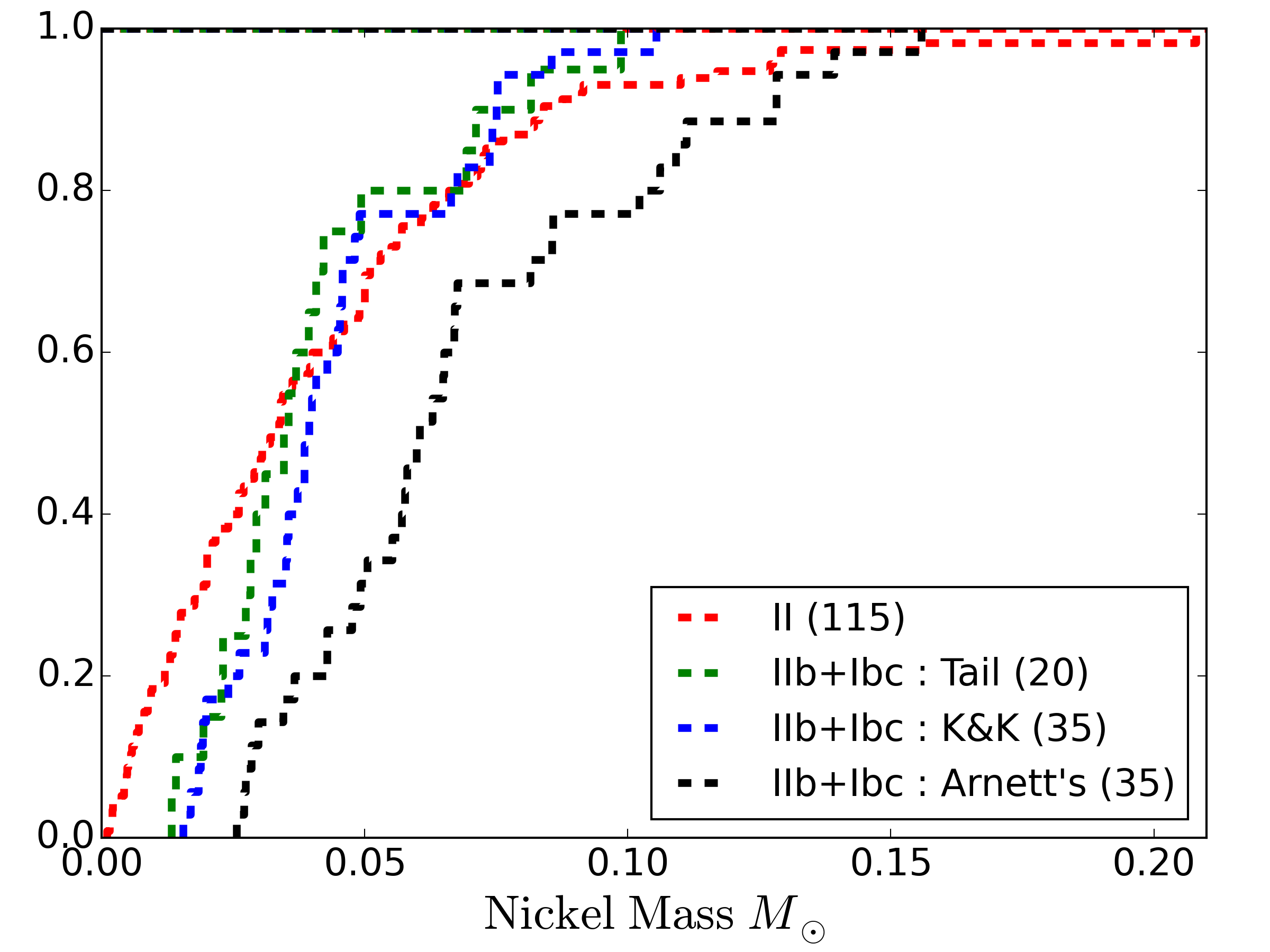
Figure 8: Cumulative distributions of the SE-SN ⁵⁶Ni masses derived through the three methods outlined in the text, but not corrected for host galaxy extinction, compared to that of SNe II (Anderson, 2019).

5 Discussion

In this work we have tested the robustness of the results and conclusions presented in Anderson (2019), i.e. that the overall ⁵⁶Ni distribution of SE-SNe is significantly larger than for SNe II. This has been achieved through concentrating on SE-SN ⁵⁶Ni masses as it was believed that these are the most uncertain. We thus defined a well-observed (in wavelength and time coverage) sample of 37 SE-SNe (14 IIb, 13 Ib, 6 Ic, 2 Ic-BL and 2 Ic-GRB), and proceeded to produce bolometric light curves and estimate ⁵⁶Ni masses.
Anderson (2019) compiled literature ⁵⁶Ni masses, where the vast majority of SE-SN values were estimated using ‘Arnett’s rule’ (Arnett, 1982), with many cases of SNe with poorly sampled photometry or epochs included. Here, we also re-estimate ⁵⁶Ni masses using Arnett’s rule, but using a small sample of SE-SNe with high quality data. When doing this, we still see much higher ⁵⁶Ni values for SE-SNe (with a smaller sample) than SNe II. A key result discussed in Anderson (2019) was the existence of a ⁵⁶Ni tail out to values as high as $>$1${\rm\ M}_{\odot}$ of ⁵⁶Ni. The sample of well-observed SE-SNe included in the present study do not show such a tail, with a highest value of 0.21${\rm\ M}_{\odot}$. Thus the SE-SN ⁵⁶Ni distribution presented here is less in conflict with explosion models (although our values are lower limits, see below for further discussion).
We then use two additional methods (Section 3.2) to estimate ⁵⁶Ni masses. The first follows Khatami & Kasen (2019) and the second uses the tail luminosity to estimate lower-limit ⁵⁶Ni masses. In both cases ⁵⁶Ni mass differences between SE-SNe and SNe II are smaller (than Arnett) but are still statistically significant.
It is often argued that the Arnett rule overestimates ⁵⁶Ni masses for many SE-SNe because of some of its limiting assumptions. This was discussed at length by Dessart et al. (2015) and Dessart et al. (2016). Those authors estimated (through detailed light curve modelling) that Arnett overestimates ⁵⁶Ni masses by 50%. However, lowering SE-SN ⁵⁶Ni masses by this amount would not remove the SN II–SE-SN ⁵⁶Ni mass difference.
Arnett’s rule and Khatami & Kasen (2019) both make significant assumptions in their formalisms, such as the degree of mixing and the value and time dependence of the ejecta opacity. In addition, both the analytic formulae used in this work and detailed light curve models in the literature assume spherical symmetry. A number of SE-SNe may arise from significantly asymmetric explosions and thus ⁵⁶Ni masses determined assuming spherical symmetry will give incorrect values. Importantly, our Tail estimates giving lower limits do not contain significant assumptions. The result that Tail ⁵⁶Ni masses for SE-SNe are still significantly higher than SNe II is thus our most robust result. Finally, we note that detailed light curve modelling of SN 1993J (e.g. Woosley et al. 1994) and SN 2011dh (e.g. Bersten et al. 2012) give ⁵⁶Ni masses that are reasonably in agreement with our estimates.
In the previous section we investigated various systematics that exist in ⁵⁶Ni mass estimation methodologies. While these systematics clearly affect ⁵⁶Ni mass estimates, we argued that none of them are likely to be large enough (and necessarily in the correct direction) to produce the observed SE-SN–SN II ⁵⁶Ni mass distribution differences. In this analysis we have concentrated our efforts on SE-SNe. We assume that the SN II ⁵⁶Ni masses in the literature (and compiled by Anderson) are robust. This assumption is based on the majority of their late-time light curves declining at the rate predicted by ⁵⁶Co (implying full trapping of the radioactive emission, in contrast to SE-SNe). Therefore, the ⁵⁶Ni mass estimation follows directly from the generalised form of equation (3): t_peak is replaced by t_epoch that is the epoch at which one measures the luminosity during the tail (the same as for the ‘Tail’ values for SE-SNe, but for SNe II these are not lower limits). Thus the method for SNe II is robust from both a theoretical and observational viewpoint.
The SN II method is still affected by the systematics discussed in Section 3. With respect to uncertainties in explosion epochs, this error still propagates to an error in the ⁵⁶Ni mass. However, this occurs at a much lower level due to the fractional uncertainty on t_epoch (at the epochs when the luminosity is measured for SNe II, $>$120 days post explosion) being much lower than the fractional uncertainty on t_peak. Host galaxy extinction estimations are just as uncertain for SNe II as they are for SE-SNe. However, de Jaeger et al. (2018) argued that apart from a few highly reddened objects most SNe II suffer from negligible extinction and colour diversity is intrinsic to the SNe themselves. Most literature studies have assumed a higher level of host extinction for SNe II than de Jaeger et al.. Thus, this systematic is more likely to push SN II ⁵⁶Ni masses to lower values: not the higher ones needed to remove the SN II–SE-SN ⁵⁶Ni difference.
SN II bolometric corrections rely heavily on the exquisite data of SN 1987A (see applications in e.g. Hamuy et al. 2003; Bersten & Hamuy 2009; Valenti et al. 2016). If other SNe II do not follow the same colour evolution as SN 1987A, the bolometric corrections employed may be in error. In Appendix B we present a first-order analysis of this issue. We estimate that the integrated flux in the range 3500-9000Å (i.e., the range generally covered by optical followup of SNe II) with respect to the flux in the $V$ band (the band often used to directly infer ⁵⁶Ni masses) varies by $\pm 0.25$ mags around the correction for SN1987A. This would translate to a dispersion of $\approx 25\%$ in SN II ⁵⁶Ni masses; however the deviations are not systematically skewed in the direction that would make SN II values larger. Thus, while a more detailed study is warranted, we do not believe that errors in bolometric corrections are the origin of our results..
Following the above summary of our work, we conclude that real, intrinsic differences exist in ⁵⁶Ni masses between SE-SNe (type IIb, Ib and Ic) and SNe II. Next, we further discuss the implications of this conclusion.

5.1 CC SN progenitors and explosions

CC SNe are spectroscopically classified into SNe II or SE SNe based on the detection of long-lasting broad hydrogen features in the former. That SE-SNe do not show these features leads to their naming: their outer hydrogen envelopes have been ‘stripped’ before explosion. How progenitor stars lose this mass has long been debated. Massive stars lose material due to winds (either steady or eruptive), and the strength of these winds increases with increasing Zero Age Main Sequence (ZAMS) mass. Thus, historically SE-SNe were generally assumed to arise from more massive progenitors than SNe II, where stellar winds are strong enough to remove the vast majority of their hydrogen envelopes and stars explode during the Wolf-Rayet phase (see e.g. Begelman & Sarazin 1986). Through this scenario the progenitors of SE-SNe have ZAMS masses higher than 25${\rm\ M}_{\odot}$, thus being significantly higher mass than SNe II.
Alternatively, the mass stripping may occur through binary interaction (e.g. Podsiadlowski et al. 1992). In this scenario SE-SN progenitors have ZAMS masses in a very similar mass range to SN II, with the presence of a close binary companion being the factor that produces distinct SN types.
During the last decade evidence has mounted in favour of the low-mass binary scenario, at least for the majority of SE-SNe. From analysis of the width of bolometric light curves around peak luminosity, a number of investigations have concluded that SE-SN ejecta masses are relatively low, implying low-mass (i.e. similar mass to SNe II) ZAMS masses (e.g. Drout et al. 2011; Taddia et al. 2015; Lyman et al. 2016; Taddia et al. 2018; Prentice et al. 2019). In addition, the relatively high rates of SE-SNe have been claimed to be incompatible with arising from only $>$25${\rm\ M}_{\odot}$ progenitors (Smith et al., 2011). While for SNe Ib and Ic there exist very few progenitor detections on pre-explosion images, there exist a small number of direct detections for SNe IIb. In all cases these progenitors are constrained to be less than 20${\rm\ M}_{\odot}$ ZAMS (Maund & Smartt, 2009; Van Dyk et al., 2013; Tartaglia et al., 2017). At the same time, studies of the local environments of SNe Ic within host galaxies suggests that these events arise from shorter lived, and therefore more massive progenitors than the rest of the CC SN population (see e.g. Anderson et al. 2012; Kangas et al. 2017; Kuncarayakti et al. 2018; Galbany et al. 2018; Maund 2018). However, the general current consensus is that at least a significant majority of SE-SN progenitors arise from binary stars with ZAMS masses similar to SNe II (see review in Smith 2014, for a detailed discussion on this topic).
Following the above, if SNe II and SE-SNe arise from similar mass progenitors then how can the ⁵⁶Ni mass differences presented here be explained? Similar mass progenitors will produce similar core structures (for the majority of events), whether the progenitor is a single star or part of a binary system. Thus, there appears to be an inconsistency between the similar-mass progenitors between different CC SNe as generally discussed in the literature, and the clear ⁵⁶Ni mass differences discussed in this paper. Further advances in our understanding of the underlying physics of different CC SN progenitors and their explosions, together with the effects of binary interaction are clearly required.

The standard explosion mechanism for CC SNe is that of neutrino driven explosions (see Müller 2016 for a recent review). As discussed in detail in Anderson (2019), several works have estimated nucleosynthetic yields within this explosion framework (e.g. Ugliano et al. 2012; Pejcha & Thompson 2015; Sukhbold et al. 2016; Suwa et al. 2019; Curtis et al. 2019). The high ⁵⁶Ni masses compiled for SE-SNe by Anderson were seen to be inconsistent with the ⁵⁶Ni values from explosion models. Here (as outlined above), for our smaller sample of well-observed SE-SNe we no longer obtain ⁵⁶Ni masses in excess of 0.2${\rm\ M}_{\odot}$, even for the Arnett values (although we again emphasise that ⁵⁶Ni masses we present in this article are lower limits due to the lack of observations outside the $B$ and $H$ bands). Thus, the degree of inconsistency between SE-SN ⁵⁶Ni masses and those predicted by neutrino-driven explosions is lowered. ⁵⁶Ni masses produced by explosion models are generally predicted to increase with increasing ZAMS mass. When compared to explosion model predictions the higher ⁵⁶Ni masses for SE-SNe than SNe II suggests higher ZAMS masses for the latter. Indeed, given that our presented ⁵⁶Ni values are lower limits, a significant fraction of the masses presented here are at the high end of explosion model predictions, possibly suggesting $>$20${\rm\ M}_{\odot}$ progenitor masses for a significant number of SE-SNe, in contradiction with the discussion above on the consensus of lower-mass binary progenitors for the majority of SE-SNe.
Recently, Ertl et al. (2019) compared their model light curves and ⁵⁶Ni mass predictions to a large number of published SE-SNe light curves (from e.g. Lyman et al. 2016; Prentice et al. 2019). These authors were not able to reproduce the observed light curves and ⁵⁶Ni estimates for a large fraction of the literature samples, through standard neutrino-driven explosions. Thus, they concluded that an additional power source is required for such SE-SNe (possibilities include a magnetar or circumstellar interaction). If an additional power source is indeed present, this would lower the required ⁵⁶Ni masses to power the light curves and thus SE-SN ⁵⁶Ni masses could become closer to those of SNe II.
From the observational side, there remains the possibility that there is a family of low ⁵⁶Ni, intrinsically dim objects that have been missed by SN searches. Indeed, (as discussed previously) the remaining ⁵⁶Ni mass difference between SE-SNe and SNe II presented in this work seems to be strongly driven by a lack of low SE-SN ⁵⁶Ni masses (see Fig. 4). If we remove SN II values below the minimum SE-SN ⁵⁶Ni mass (0.015M_⊙, for SN 2017czd) the distributions become statistically consistent, with KS p-values greater than 40% (except for Arnett’s values that remain discrepant; p-value below $10^{-3}$). However, we once again reiterate that our ⁵⁶Ni values are strict lower limits. If we arbitrarily increase our SE-SN ⁵⁶Ni values by 20% (roughly accounting for the missing flux outside our filter range), a small tension remains; between the Khatami SE-SN and SN II distributions a KS test gives a p-value of 9%.
There is now significant evidence that the majority of massive stars are found in binary systems where their orbital periods are such that significant interaction with the companion star will occur during the star’s life (e.g. Sana et al. 2012). There is also some indication of an increasing relative fraction of short period systems in late-B and O-type stars (Moe & Di Stefano, 2017). Such observations imply that some SE-SNe may originate from quite low-mass massive stars. At the lowest mass range (i.e. the lowest masses from which stars will still explode as CC SNe) it is possible that such progenitors explode with small ejecta masses and little ⁵⁶Ni.
This lack of low-mass ⁵⁶Ni SE-SNe in current samples begs the question: if a SE-SN were to explode with a ⁵⁶Ni mass of 0.001${\rm\ M}_{\odot}$ (the extreme lower end of the SN II distribution, Müller et al. 2017; Anderson 2019) how dim and fast evolving would such an event be and would current surveys detect such explosions?
Scenarios for these type of objects exist in theory (Kleiser & Kasen, 2014; Tauris et al., 2015), and a few transients, associated with the family of “Calcium gap” events and potential precursor systems of binary neutron star mergers, have been observed recently (De et al., 2018a, b; Shen et al., 2019). The latter class, named ultra-stripped SNe, arise from tight (period $<2$ days) binary sytems of a Helium star and a compact object (such as a neutron star). The pre-SN star would contain less than 0.2M_⊙ of helium in the envelope and the final explosion would eject $\approx 0.1$${\rm\ M}_{\odot}$, with a ⁵⁶Ni mass of $\approx 0.01$${\rm\ M}_{\odot}$ (see e.g. Moriya et al. 2017). Ultra-stripped SNe are expected to have a very fast evolution (rise time of less than 10 days) and to be very dim - with the exception of progenitors with a pre-SN extended progenitor or when the SN ejecta interacts with CSM (Kleiser & Kasen, 2014; Kleiser et al., 2018). The rate for ultra-stripped SNe is expected to be 1% of all CCSNe, and therefore their inclusion in the current study is unlikely to significantly reduce the SN II–SE-SN ⁵⁶Ni mass difference. Future modelling of low-mass binary systems producing low-⁵⁶Ni mass CC SNe is certainly warranted.

6 Conclusions

The amount of radioactive material synthesised in a SN explosion is a fundamental parameter that determines the transient behaviour of all SN types. The mass of ⁵⁶Ni produced in CC SNe is determined by the core-structure at the explosion epoch, together with the explosion energy. Therefore constraining ⁵⁶Ni masses for different CC SN types can shed light on differences in progenitors and explosion properties.
We conclude that real intrinsic differences in ⁵⁶Ni mass exist between observed SE-SNe and SNe II, differences that persist when different systematic errors in ⁵⁶Ni mass estimations are analysed. In particular, a ⁵⁶Ni mass difference is still observed when we use the radioactive tail luminosities to obtain ⁵⁶Ni mass lower limits. This Tail methodology is extremely robust and we suggest that effort is made to obtain additional well-sampled multi-colour late time observations of SE-SNe. The ⁵⁶Ni discrepancy we present in this work is driven by a lack of low ⁵⁶Ni mass SE-SNe.
That SE-SNe are observed to produce larger ⁵⁶Ni masses than SNe II implies significant differences in their progenitor properties and/or explosion mechanisms. A full understanding of which parameter produces these ⁵⁶Ni mass differences is of utmost importance for our understanding of massive star explosions.

———————————————–

Appendix A Sample properties

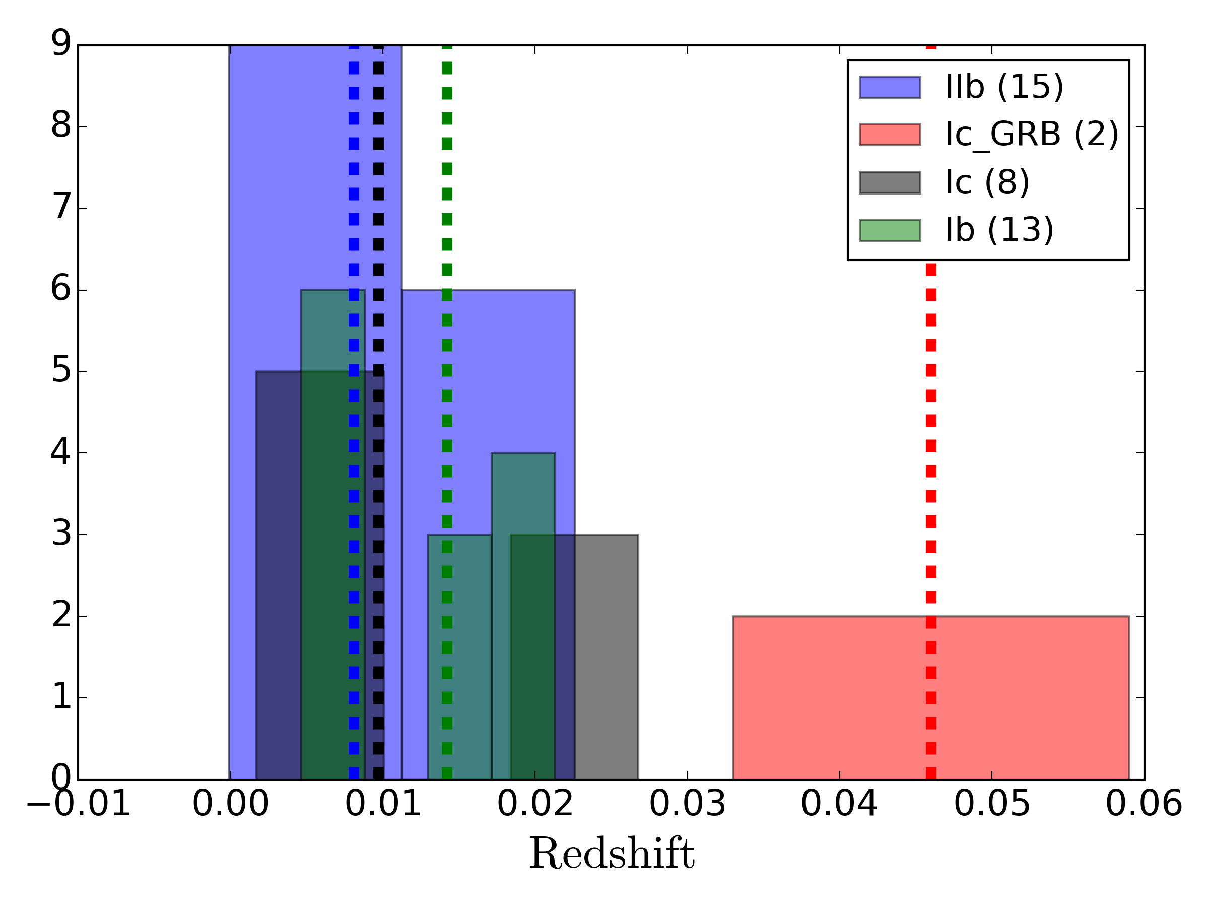
Figure 9: Heliocentric redshift distribution of our $BVRIYJH$ sample. Each SN subtype is colour labeled and a vertical line of the same colour is used to mark the median of that distribution.

Table 2 lists the SE-SNe used in this work, together with their types, and various other relevant parameters. With the exception of a couple SNe associated with a gamma ray burst or X-ray flash, the sample has a low redshift ($z\leq 0.03$), and the redshift distribution is presented in Fig. 9. The time range between the last non detection and the discovery epoch is on average less than two weeks for the sample of this work, which corresponds to an approximate mean error in explosion epochs of less than seven days.

Table 2: Sample of SE SNe used in this work. Selection criteria for this sample is described in Section 2.

SN	Type	Host	Host redshift(+)	Host $d_{L}^{({\dagger})}$	MW $E(B-V)$	Host $E(B-V)^{(*)}$	$t_{0}$	References
SN1993J	IIb	M81	-0.00011	3.63	0.07	0.10	49073.50	(a)
SN2004ex	IIb	NGC0182	0.01755	70.60	0.02	0.08	53287.90	(CSP)
SN2004ff	IIb	ESO-552-G040	0.0226	92.70	0.03	0.10	53297.66	(CSP)
SN2004gq	Ib	NGC1832	0.006468	25.10	0.06	0.08	53346.87	(CSP),(Cfa)
SN2004gv	Ib	NGC0856	0.019973	79.60	0.03	0.03	53345.27	(CSP)
SN2005aw	Ic	IC4837A	0.009498	41.50	0.05	0.21	53445.67	(CSP)
SN2005em	Ic	IC0307	0.025981	105.00	0.08	0.00	53635.00	(CSP)
SN2005hg	Ib	UGC1394	0.02131	86.00	0.09	None	53665.75	(CSP)
SN2005kl	Ic	NGC4369	0.003485	21.57	0.02	None	53686.14	(Cfa)
SN2005mf	Ic	UGC4798	0.02676	113.00	0.01	None	53723.33	(Cfa)
SN2006aj	Ic-GRB	A032139+1652	0.033	132.40	0.13	0.00	53784.15	(Cfa),(b)
SN2006ba	IIb	NGC2980	0.01908	82.70	0.04	0.10	53801.11	(Cfa),(CSP)
SN2006ep	Ib	NGC0214	0.015134	61.90	0.03	None	53975.49	(Cfa),(CSP)
SN2006fo	Ib	UGC02019	0.020698	82.70	0.02	0.21	53983.36	(Cfa),(CSP)
SN2006lc	Ib	NGC7364	0.016228	59.20	0.06	0.36	54014.74	(Cfa),(CSP)
SN2006T	IIb	NGC3054	0.008091	31.60	0.06	0.14	53757.64	(Cfa),(CSP)
SN2007C	Ib	NGC4981	0.005604	21.00	0.04	0.43	54095.44	(Cfa),(CSP)
SN2007gr	Ic	NGC1058	0.0017	9.29	0.09	0.03	54325.00	(Cfa),(c)
SN2007kj	Ib	NGC7803	0.017899	72.50	0.07	0.00	54363.61	(Cfa),(CSP)
SN2007uy	Ib	NGC2770	0.0065	31.33	0.02	0.63	54462.33	(Cfa),(d)
SN2007Y	Ib	NGC1187	0.004637	18.40	0.02	0.00	54145.00	(CSP),(e)
SN2008aq	IIb	MCG-02-33-020	0.007972	26.90	0.04	0.00	54510.79	(Cfa),(CSP)
SN2008ax	IIb	NGC4490	0.0019	9.20	0.02	0.28	54528.30	(Cfa),(f)
SN2008D	Ib	NGC2770	0.0065	31.33	0.02	0.63	54474.50	(Cfa),(g)
SN2008hh	Ic	IC0112	0.01941	77.70	0.04	0.00	54780.69	(Cfa),(CSP)
SN2009bb	Ic-BL	NGC3278	0.00988	39.80	0.09	0.48	54909.10	(CSP),(h)
SN2009iz	Ib	UGC02175	0.01419	58.60	0.07	None	55083.00	(Cfa)
SN2009jf	Ib	NGC7479	0.0079	33.73	0.10	0.05	55099.00	(Cfa),(i)
SN2009K	IIb	NGC1620	0.011715	44.10	0.05	0.06	54843.57	(Cfa),(CSP)
SN2010as	IIb	NGC6000	0.0073	27.16	0.15	0.42	55270.75	(j)
SN2010bh	Ic-GRB	A071031-5615	0.059	244.34	0.10	0.14	55271.53	(k)
SN2011fu	IIb	UGC1626	0.019	74.47	0.07	0.01	55824.00	(l)
SN2011dh	IIb	M51	0.002	7.87	0.03	0.05	55712.50	(m)
SN2011hs	IIb	IC5267	0.0057	24.10	0.01	0.16	55871.50	(n)
SN2013df	IIb	NGC4414	0.0024	21.37	0.02	0.08	56447.30	(o)
SN2016coi	Ic-BL	UGC11868	0.00364	17.20	0.07	0.12	57532.50	(p)
SN2017czd	IIb	UGC9567	0.00835	32.00	0.02	0.00	57845.00	(q)

Table 3: Peak parameters of our $BVRIYJH$ light curves and the ⁵⁶Ni masses obtained as described in Section 3. All our luminosities and nickel masses are lower limits, as described in the manuscript. For the Khatami & Kasen (2019) ⁵⁶Ni values we use their reccomended $\beta$ values, of 0.82 for SNe IIb, and $9/8$ for SNe Ib and SNe Ic (including SNe Ic-BL).

SN	Type	$t_{p}\ [days]$	$L_{p}\ [10^{41}erg/s]$	Arnett  $[M_{\odot}]$	K&K  $[M_{\odot}]$	Tail  $[M_{\odot}]$
SN1993J	IIb	21.89	17.20	0.10	0.06	0.05
SN2004ex	IIb	20.86	13.34	0.08	0.04	0.05
SN2004ff	IIb	15.33	19.00	0.08	0.05	None
SN2004gq	Ib	12.42	13.81	0.05	0.04	0.05
SN2004gv	Ib	22.38	18.79	0.12	0.08	None
SN2005aw	Ic	12.01	27.48	0.10	0.07	None
SN2005em	Ic	13.43	15.66	0.06	0.05	None
SN2005hg	Ib	18.93	19.63	0.10	0.07	0.07
SN2005kl	Ic	18.49	6.57	0.03	0.02	0.02
SN2005mf	Ic	10.98	15.45	0.05	0.04	None
SN2006aj	Ic-GRB	10.18	50.24	0.15	0.12	None
SN2006ba	IIb	20.91	13.77	0.08	0.04	None
SN2006ep	Ib	14.58	10.32	0.04	0.03	None
SN2006fo	Ib	24.53	28.93	0.20	0.13	None
SN2006lc	Ib	25.98	17.11	0.12	0.08	None
SN2006T	IIb	23.53	16.19	0.11	0.06	0.05
SN2007C	Ib	20.45	10.94	0.06	0.04	0.03
SN2007gr	Ic	13.22	12.97	0.05	0.04	0.03
SN2007kj	Ib	18.16	10.35	0.05	0.04	0.03
SN2007uy	Ib	19.36	37.94	0.21	0.14	0.10
SN2007Y	Ib	20.18	4.81	0.03	0.02	None
SN2008aq	IIb	20.59	6.25	0.04	0.02	0.02
SN2008ax	IIb	21.87	7.68	0.05	0.02	0.02
SN2008D	Ib	20.42	13.96	0.08	0.05	0.04
SN2008hh	Ic	11.18	17.38	0.06	0.04	None
SN2009bb	Ic-BL	12.77	44.62	0.17	0.12	0.08
SN2009iz	Ib	28.84	12.85	0.10	0.07	0.07
SN2009jf	Ib	21.65	28.16	0.17	0.12	0.11
SN2009K	IIb	27.06	19.95	0.15	0.08	None
SN2010as	IIb	17.68	30.46	0.15	0.09	0.09
SN2010bh	Ic-GRB	9.24	37.86	0.11	0.09	None
SN2011fu	IIb	22.30	23.24	0.14	0.08	None
SN2011dh	IIb	20.25	11.01	0.06	0.03	0.04
SN2011hs	IIb	17.29	8.49	0.04	0.02	None
SN2013df	IIb	21.92	16.28	0.10	0.05	0.06
SN2016coi	Ic-BL	19.49	25.87	0.14	0.10	0.10
SN2017czd	IIb	14.50	6.22	0.03	0.02	None

A.1 SE SN rise times and ⁵⁶Ni systematics as measured at the peak.

In Fig. 10 we show the rise time distributions obtained for the different SNe sub-types. As expected, the shorter rise times belong to the SNe Ic (including Ic-BL) while the rise times for SN types Ib/IIb are higher. The effect of the rise time and mixing (as measured by the $\beta$ parameter) on the ratio of the ⁵⁶Ni mass measured with the Khatami & Kasen and the Arnett method is shown in Fig. 11, where we show a 2D colour plot with the dependence of this ratio. In most of the parameter space Arnett’s rule gives a relative overestimate (compared to Khatami & Kasen), while for short rise times and higher mixing Arnett’s rule is comparable to the Khatami & Kasen method. Considering the rise times of our sample, we expect that the parameter space where Arnett’s rule is more accurate is covered by SN types Ic/Ic-BL SNe, while for SNe IIb we expect that Arnett’s rule will always be an overestimation.

Appendix B Nebular bolometric corrections for SNe II

Bersten & Hamuy (2009) explored bolometric corrections (BCs) at nebular epochs for SN II, finding that considering the $U-K$ bands the BC of SN 1987A roughly agrees with the SNe II 1999em and 2003hn, within a range of $\pm 0.25$ mags. We further test this conclusion here.
We used nebular-phase spectra of SN 1987A and a sample of 18 SNe II, including one peculiar object (SN 2009E). Together with nebular spectra from models of Jerkstrand et al. (2012) and Dessart et al. (2013), we cover a wide range in expected physical progenitor properties, such as progenitor mass and metalicity, for red supergiants (the presumed progenitors of SNe II). Spectra used cover from 150 to 300 days past explosion with a wavelength range of 3500-9000Å. With this sample the fraction of integrated flux in the range 3500-9000Å ($F(3500-9000)$) with respect to the flux in the $V$ band was estimated, which we name the pBC (pseudo-bolometric-correction):

$$pBC=-2.5log(F(3500-9000)/F_{V})$$ (6)

The estimated pBCs from observations span $\pm 0.15$ magnitudes around the correction for SN 1987A (Fig. 12.1), which is very close to the sample mean. The pBC mean of the models is 0.12 mags from SN1987A and observations. We found that the $3\sigma$ dispersion from observations is 0.26 mags, which translates to a dispersion of $\approx 25\%$ in SN II ⁵⁶Ni mass. Although significant, this cannot explain the differences obtained in this work, because the deviations are not systematically skewed toward the direction that would make SN II ⁵⁶Ni masses larger. Thus, through this analysis we conclude that using the bolometric correction from SN 1987A to estimate SN II ⁵⁶Ni masses does not produce a systematic that is biasing our results.

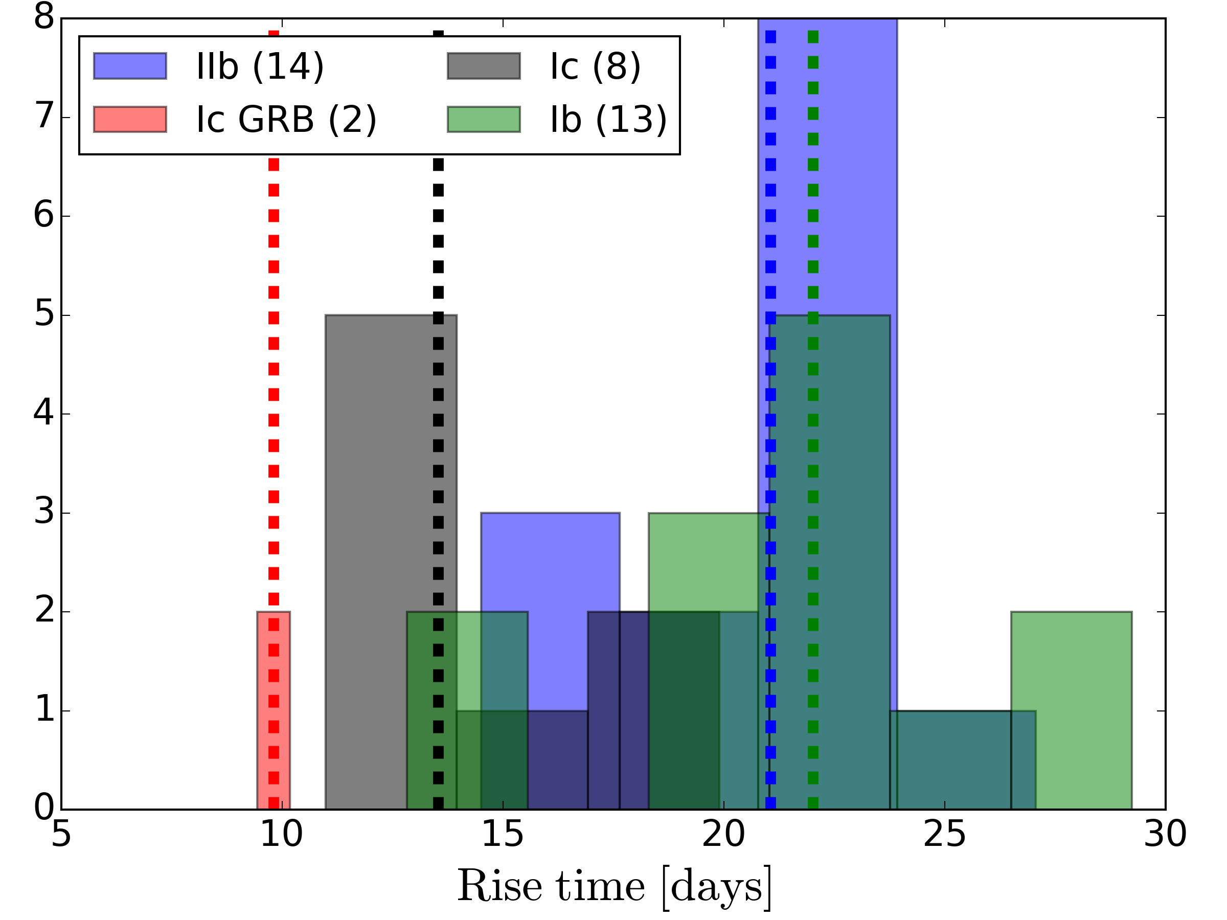
Figure 10: Rise time distribution of our $BVRIYJH$ sample. Each SN subtype is colour labeled and a vertical line of the same colour is used to mark the median of that distribution.

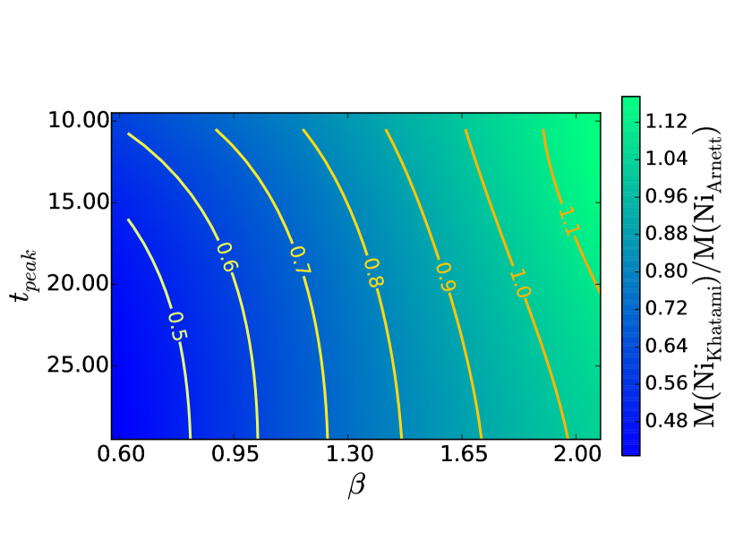
Figure 11: Colour plot showing the ratio of the ⁵⁶Ni mass measured using the Khatami & Kasen (2019) method to the one measured with the Arnett’s rule, as a function of the peak time and the $\beta$ parameter.

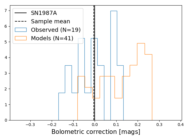
Figure 12: Pseudo-bolometric corrections at the nebular phase for SNe II. These were calculated using observed spectra from 18 SNe, with epochs ranging from 150 to 300 days past explosion and models from (Jerkstrand et al. 2012) and Dessart et al. (2013).

Appendix C $BVRIYJH$ pseudo-bolometric light curves and ⁵⁶Ni mass measurements

We now present the full sample of pseudo-bolometric light curves of our SE-SNe, obtained from the integration of the flux in the $BVRIYJH$ (or equivalent) bands as described in Section 3. These light curves are presented in Figs B.1 through B.7.

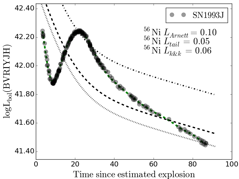
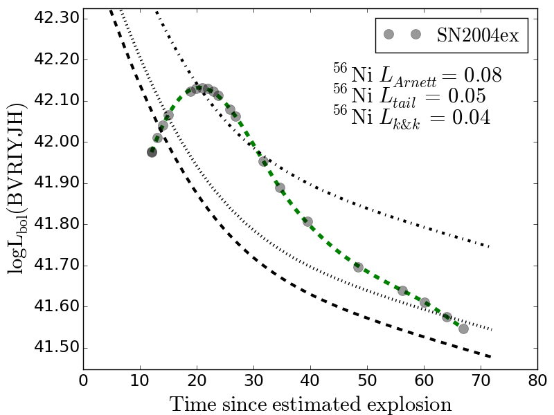
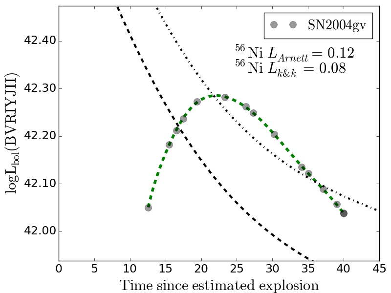
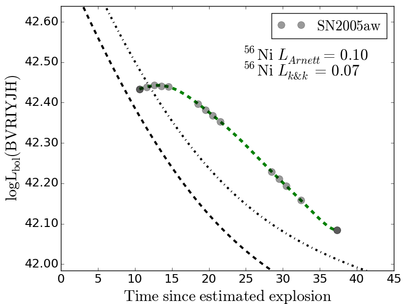
Figure 13: $BVRIYJH$ pseudo-bolometric light curves for SE-SNe. The dotted lines give the ⁵⁶Ni mass decay curve for that estimated through the Tail. The dashed line gives the ⁵⁶Ni mass decay curve from Khatami & Kasen, while the dot-dashed line gives that from Arnett.

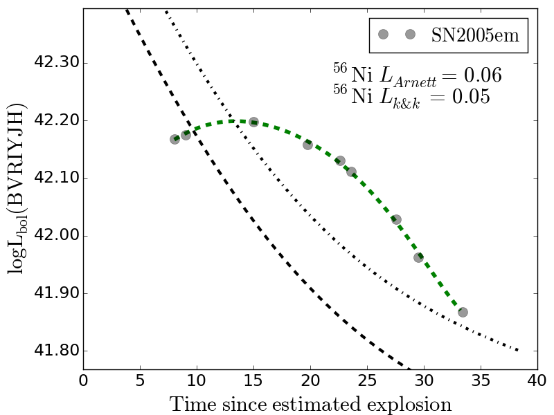
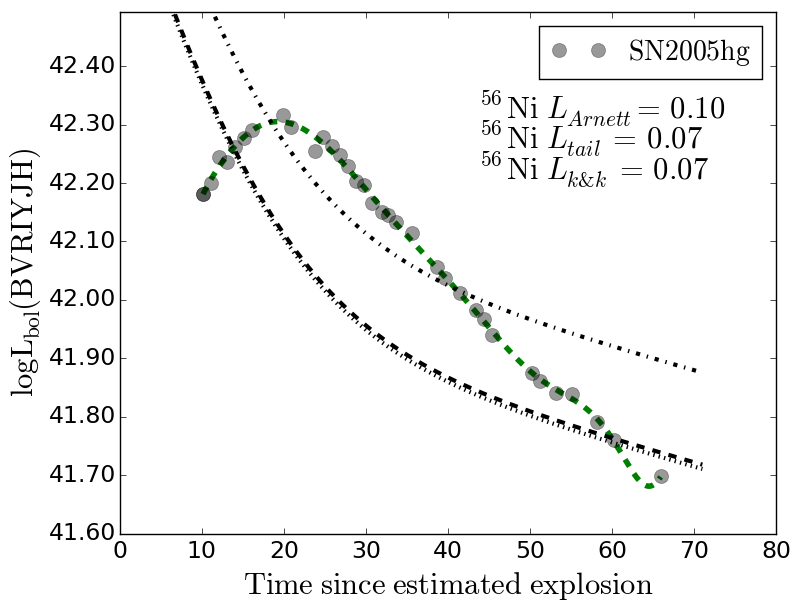
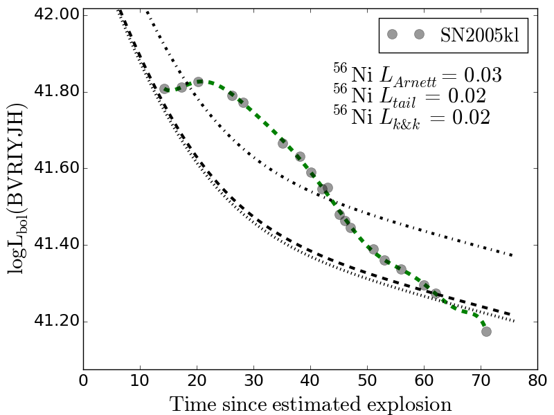
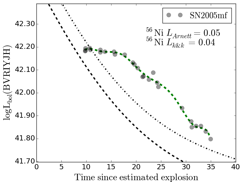
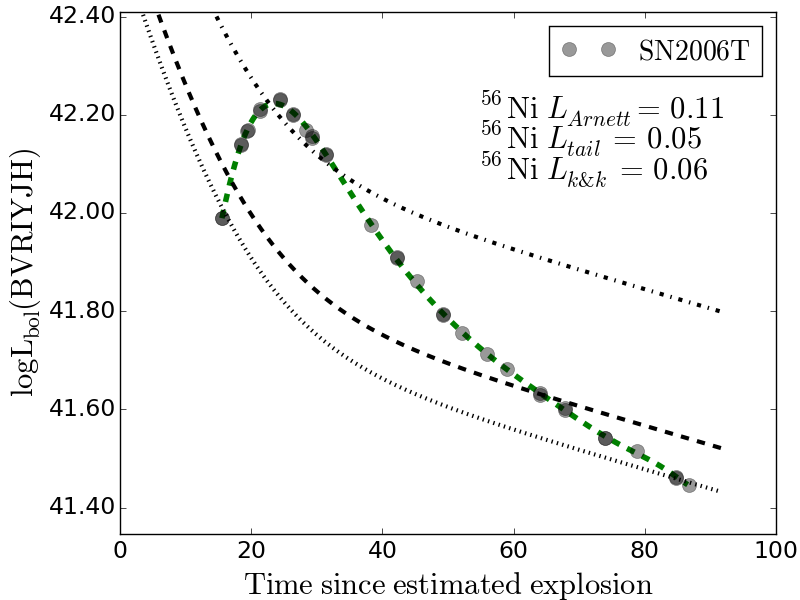
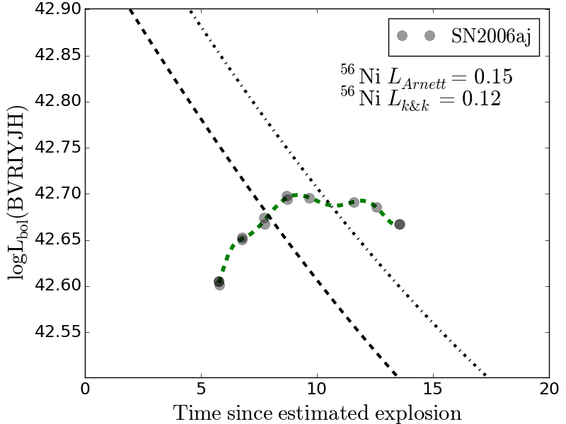
Figure 14: $BVRIYJH$ pseudo-bolometric light curves for SE-SNe. The dotted lines give the ⁵⁶Ni mass decay curve for that estimated through the Tail. The dashed line gives the ⁵⁶Ni mass decay curve from Khatami & Kasen, while the dot-dashed line gives that from Arnett.

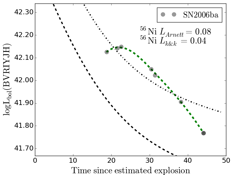
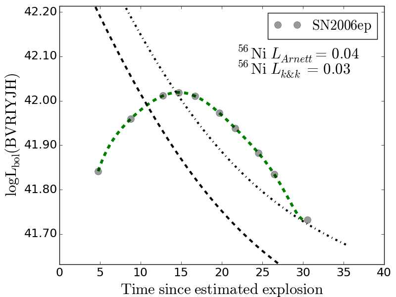
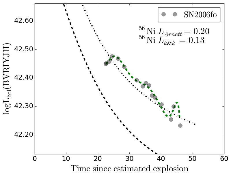
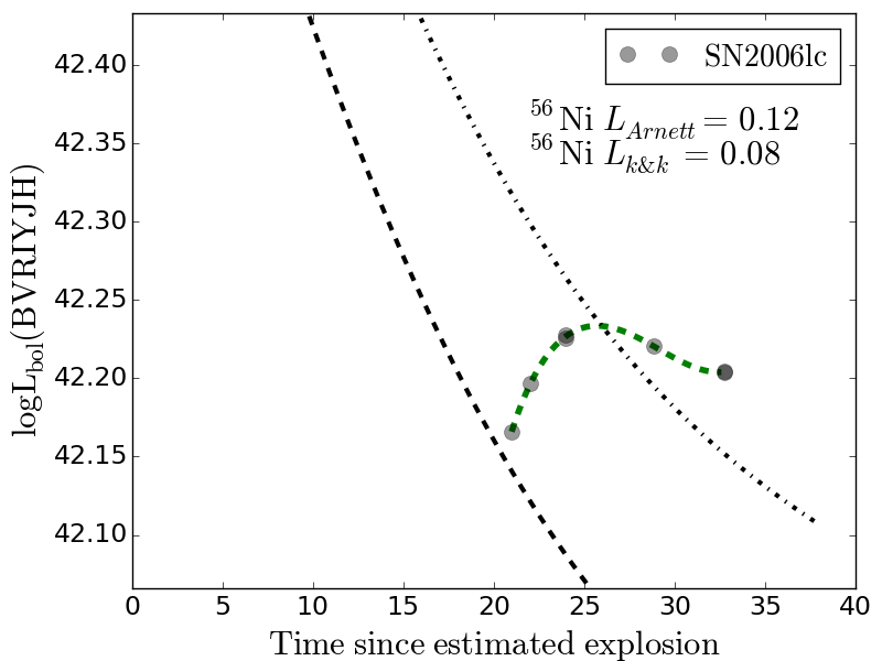
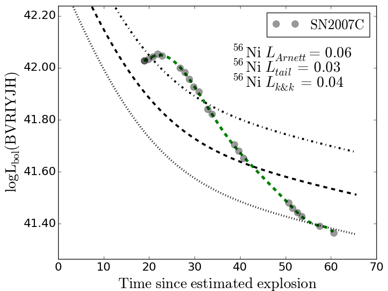
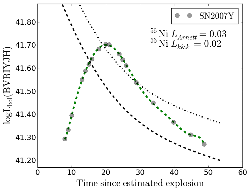
Figure 15: $BVRIYJH$ pseudo-bolometric light curves for SE-SNe. The dotted lines give the ⁵⁶Ni mass decay curve for that estimated through the Tail. The dashed line gives the ⁵⁶Ni mass decay curve from Khatami & Kasen, while the dot-dashed line gives that from Arnett.

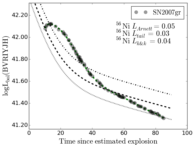
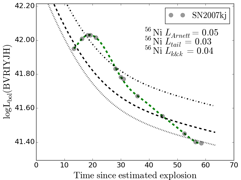
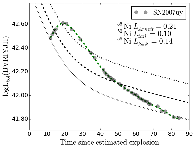
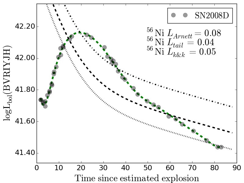
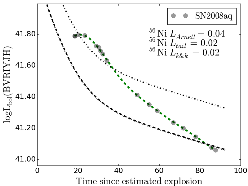
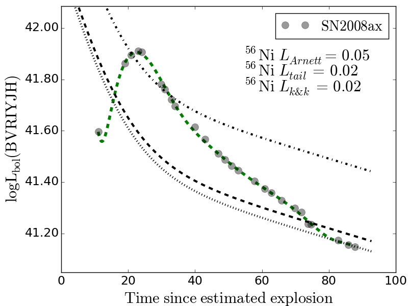
Figure 16: $BVRIYJH$ pseudo-bolometric light curves for SE-SNe. The dotted lines give the ⁵⁶Ni mass decay curve for that estimated through the Tail. The dashed line gives the ⁵⁶Ni mass decay curve from Khatami & Kasen, while the dot-dashed line gives that from Arnett.

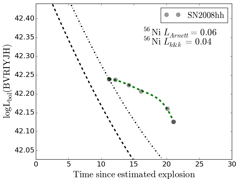
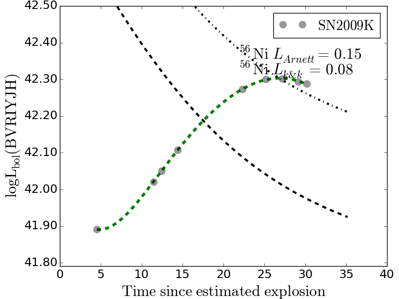
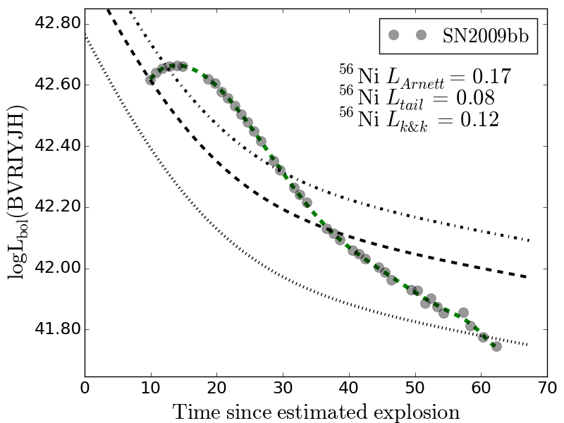
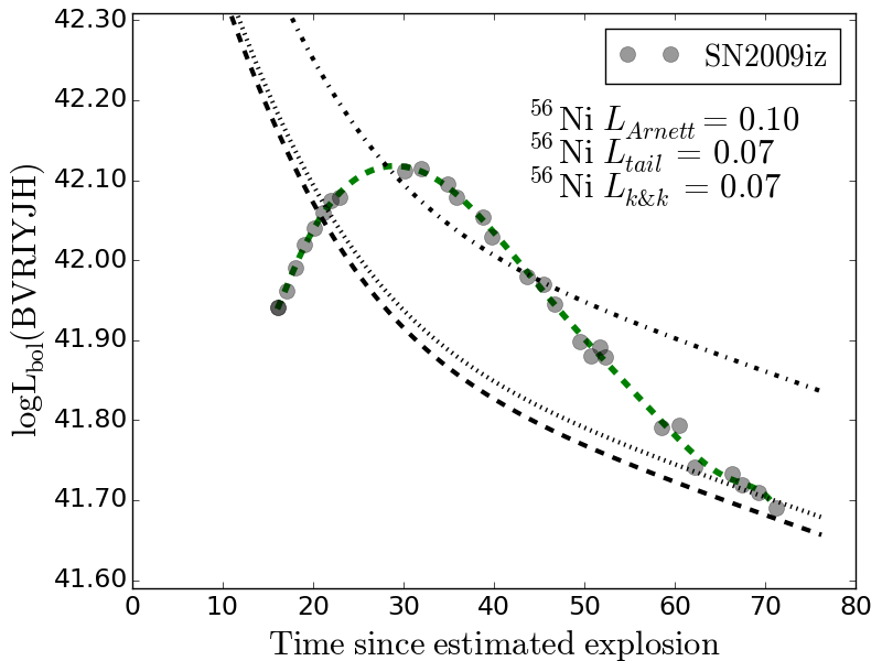
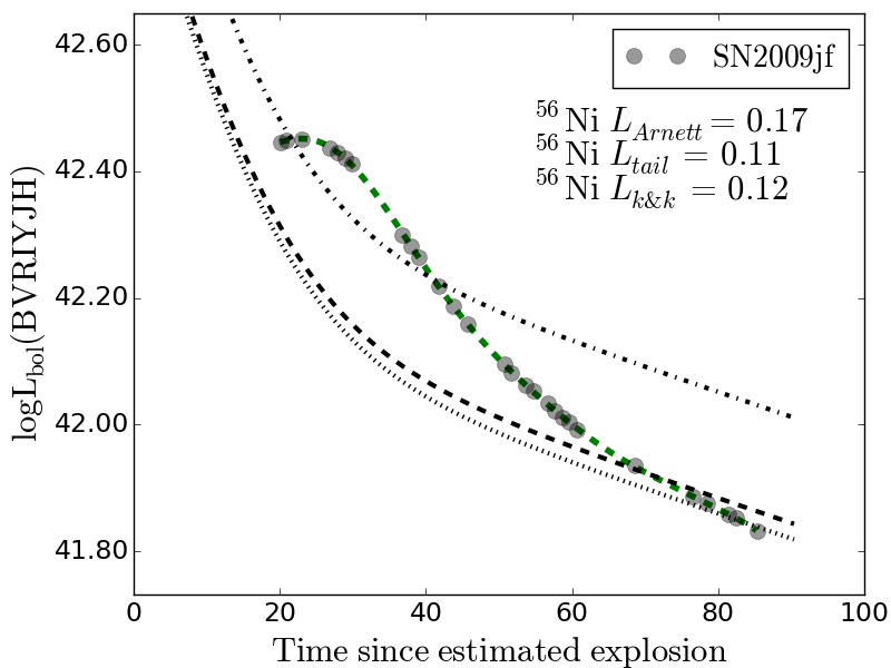
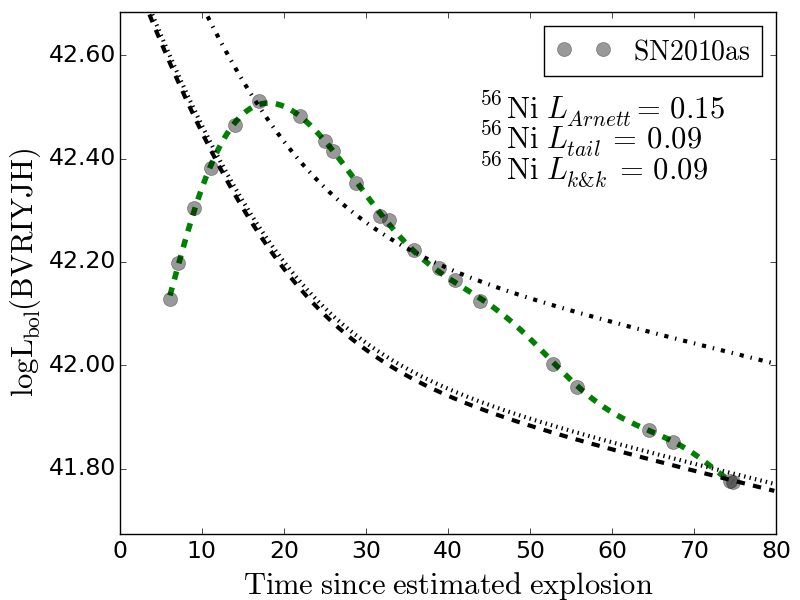
Figure 17: $BVRIYJH$ pseudo-bolometric light curves for SE-SNe. The dotted lines give the ⁵⁶Ni mass decay curve for that estimated through the Tail. The dashed line gives the ⁵⁶Ni mass decay curve from Khatami & Kasen, while the dot-dashed line gives that from Arnett.

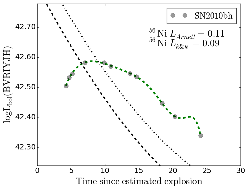
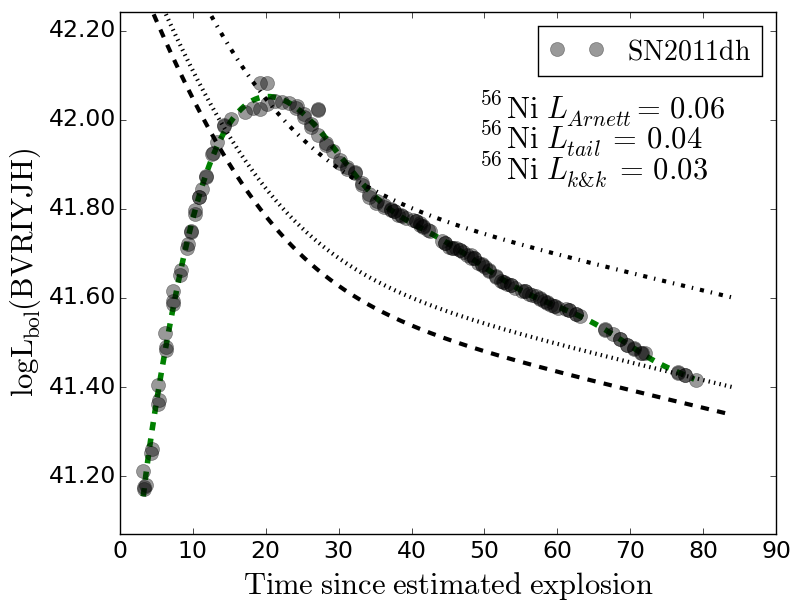
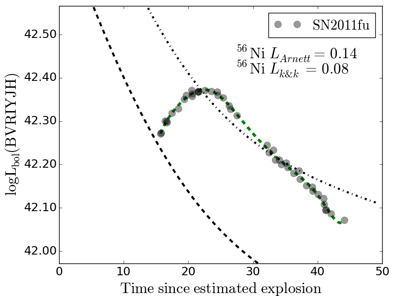
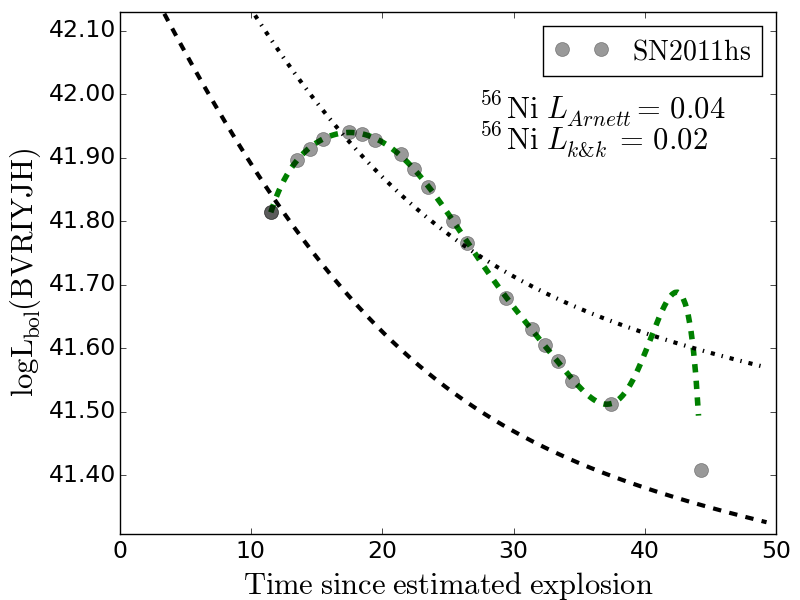
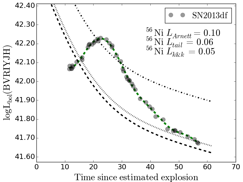
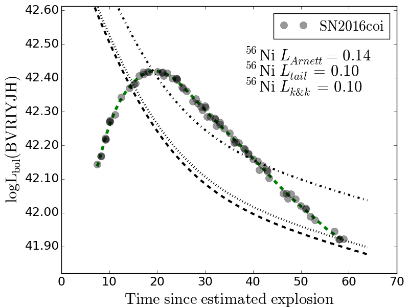
Figure 18: $BVRIYJH$ pseudo-bolometric light curves for SE-SNe. The dotted lines give the ⁵⁶Ni mass decay curve for that estimated through the Tail. The dashed line gives the ⁵⁶Ni mass decay curve from Khatami & Kasen, while the dot-dashed line gives that from Arnett.

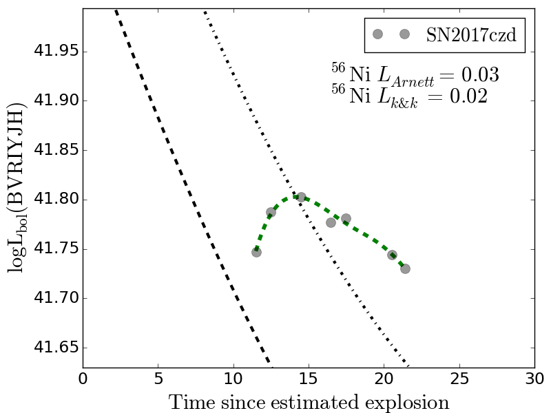
Figure 19: $BVRIYJH$ pseudo-bolometric light curves for SE-SNe. The dotted lines give the ⁵⁶Ni mass decay curve for that estimated through the Tail. The dashed line gives the ⁵⁶Ni mass decay curve from Khatami & Kasen, while the dot-dashed line gives that from Arnett.